Submitted:
15 October 2025
Posted:
16 October 2025
You are already at the latest version
Abstract
In this article, we examine the dynamic interdependencies among components of Japan's consumer price index (CPI) using a two-lag time-varying factor loading (TLTVFL) model. Whereas previous studies have typically decomposed CPI series into long-term trends, seasonal patterns, and cyclical fluctuations, such approaches mainly describe structural features without fully uncovering the latent mechanisms that drive price dynamics. The proposed TLTVFL framework addresses this limitation by allowing both factor loadings and their lagged effects to evolve over time, thereby capturing gradual structural changes and the time-varying propagation of shocks across CPI categories. Using monthly data for ten major CPI categories from January 1970 to December 2024, we identify evolving common factors, category-specific sensitivities, and dynamic transmission patterns associated with major macroeconomic events. The findings reveal substantial temporal variation in inter-category linkages, offering fresh insights into sectoral contributions to inflationary pressures and providing policy-relevant implications for more effective monetary and fiscal interventions. Methodologically, this study extends the frontier of dynamic factor modeling, while empirically, it deepens the understanding of the mechanisms underlying price fluctuations over a long historical horizon.
Keywords:
consumer price index
; inflation dynamics
; Japanese economy
; monetary policy
; structural change
; time-varying factor loading model
1. Introduction
Understanding the detailed mechanisms underlying economy-wide price fluctuations is essential for monitoring inflationary pressures, assessing business-cycle phases, and formulating effective price-stabilization policies. Boskin et al. (1998) emphasize that “accurately measuring prices and their rate of change—namely inflation—is central to almost every economic issue; there is virtually no other issue so endemic to every field of economics.” Although several indicators are used to measure price levels, the consumer price index (CPI) remains the most widely employed gauge of inflation (Ito and Hoshi, 2020, Ch. 6). Accordingly, this study focuses on the dynamics of the CPI.
Specifically, we investigate the mechanisms driving fluctuations in Japan’s category-level CPIs using the two-lag time-varying factor-loading (TLTVFL) model proposed by Kyo and Noda (2025a). While the aggregate CPI is commonly used in empirical and policy analysis, it often masks substantial heterogeneity across sectors, making it difficult to capture category-specific dynamics and the interactions that shape overall price movements (Blinder, 1982; Bryan and Cecchetti, 1993; Hale and Jordà, 2007). This underscores the need for analytical approaches that move beyond aggregate indicators and explicitly account for interdependencies among disaggregated CPI components.
Previous research has attempted to address this issue by decomposing CPI series into structural components such as long-term trends, seasonal effects, and cyclical variations (Harvey, 1990; Baxter and King, 1999). Kyo and Noda (2025b) decompose the CPIs of ten major Japanese categories into trend, seasonal, and cyclical elements to examine the characteristics of each type of fluctuation. Their analysis relies on the moving-linear (ML) modeling framework introduced by Kyo and Kitagawa (2023) and its extended version developed by Kyo et al. (2024). Among these components, the trend and cyclical terms are particularly informative. The trend captures long-run movements in the CPI and is relatively straightforward to interpret, whereas the cyclical component reflects short-term, category-specific fluctuations as well as common cyclical movements across categories. These cyclical dynamics contain valuable information about sectoral policy effects and shared business-cycle behavior.
Building on this perspective, the present study focuses on the cyclical components of category-level CPIs and applies the TLTVFL model to examine their dynamic interactions. The TLTVFL model is a multivariate factor-analysis framework in which each variable is associated with a common factor through two lagged terms, each with time-varying loadings. Unlike static factor models or standard state-space representations, the TLTVFL model allows factor loadings to evolve over time, thereby capturing gradual structural changes and the dynamic propagation of shocks. This feature makes it especially suitable for long historical series subject to structural breaks—conditions frequently observed in Japan’s price system. Compared with Bayesian Gaussian-process approaches (e.g., Stock and Watson, 2016) and traditional dynamic-factor (DF) models (e.g., Stock and Watson, 1989, 1991), the TLTVFL framework provides a flexible yet computationally tractable means of representing time-varying interdependencies.
Our empirical analysis employs monthly data for ten major CPI categories from January 1970 to December 2024, encompassing major macroeconomic episodes such as the oil crises, the asset-price bubble, prolonged deflation, and the COVID-19 pandemic. Using the TLTVFL model, we address the following questions: What common fluctuations emerge among the cyclical components of different categories? How have common factors and category-specific sensitivities evolved over time? What patterns characterize the transmission of shocks across categories? And how are these dynamic structures linked to broader business cycles and policy regimes in the Japanese economy?
This study makes four principal contributions. First, it develops an indicator that captures price-fluctuation patterns diverging from those of the aggregate CPI. Second, it advances methodological practice by introducing a framework for modeling dynamic interdependencies in high-dimensional macroeconomic data. Third, it provides novel empirical evidence on the evolution of sectoral price linkages in the Japanese economy over the past five decades. Finally, it offers policy-relevant insights into the sources of inflationary pressures and the propagation of shocks, thereby informing the design of more effective stabilization policies. To the best of our knowledge, no previous research has examined CPI fluctuations from a comparable perspective.
The main findings can be summarized as follows. The TLTVFL model reveals dynamic linkages among disaggregated CPI categories that are obscured in the aggregate index. It identifies differences in leading, coincident, and lagging relationships across categories and traces structural changes in sectoral sensitivities to the common factor over the past five decades. These results suggest that sector-level price dynamics can provide early warnings of inflationary pressures and offer new empirical evidence for developing more timely and targeted policy interventions.
2. Methodology
2.1. Major Categories of the CPI
In Japan, the CPI is classified into ten major categories, as shown in Table 1.
In this study, the cyclical component of each category is extracted and treated as a separate variable. Accordingly, the analysis is conducted with ten variables in total, corresponding to the ten CPI categories.
2.2. The TLTVLF Model
Let denote the dataset of variables within the context of our framework. The model is specified as
where is the i-th variable, is the common factor, and , are its values at lags and . The coefficients and are time-varying factor loadings (TVFLs), and is the idiosyncratic component. Throughout this article, is assumed unless stated otherwise, where N denotes the sample size. The specification in Equation (1) is referred to as the two-lag time-varying loading factor (TLTVLF) model, originally proposed by Kyo and Noda (2025a) for analyzing business cycle mechanisms.
This framework allows examination of lead–lag relationships between the variables and the common factor. For simplicity, we fix and focus on . If , the i-th variable leads the common factor, suggesting a causal role in price fluctuations. When , the variable lags behind, reflecting the consequences of fluctuations. Moreover, if , the variable is nearly coincident. Combinations of and introduce more complex dynamics, which are discussed later. In addition, the sign and magnitude of the TVFLs indicate the direction and strength of the common factor’s influence, and their evolution over time reveals changes in interdependencies.
The TLTVLF model has two defining features: (1) Each variable is linked to the common factor through two lagged terms, facilitating the analysis of causal relationships. (2) The factor loadings vary over time, enabling the model to capture structural changes in the dependence between the common factor and individual variables. Additionally, it is worth noting that these features enhance monitoring of CPI dynamics and provide a more detailed understanding of fluctuation mechanisms.
Relative to Stock-Watson type dynamic factor (DF) models, the framework based on the TLTVLF model differs in two key respects as follows: (1) The DF models difference variables to remove trends, whereas the TLTVLF model uses decomposed cyclical components, avoiding information loss. (2) The DF models typically apply autoregressive structures to both common and idiosyncratic factors, while the TLTVLF model introduces lags into the common factor and employs time-varying loadings, thereby simplifying structural analysis. Although the TLTVLF modeling approach requires specialized estimation techniques, this challenge can be addressed within the distribution-free dynamic linear modeling framework (Kyo and Noda, 2025c).
Stock and Watson (2009) and Su and Wang (2017) have also introduced time-varying factor loadings. The former emphasized sudden shocks, whereas the latter focused on continuous structural change. While similar in principle, these approaches remain within general factor analysis frameworks and face estimation difficulties, whereas the TLTVLF model is specifically designed for business cycle analysis.
In the TLTVLF model, the two factor loadings and their associated lags must be estimated simultaneously, which makes the estimation procedure and algorithm complex. Once these parameters are estimated, the common factor can be derived as a byproduct. For further details, see Kyo and Noda (2025a).
2.3. Application of the TLTVLF Model
2.3.1. Constructing the Cyclical Price Factor Index
The common factor estimated using the TLTVLF model captures the co-movements embedded in the cyclical components of each CPI category. Its estimates therefore provide a basis for analyzing short-term CPI variations, such as the direction of price movements and the dynamics of business cycles.
Because the common factor is standardized with mean zero and variance one, its numerical values serve only as a relative indicator of economic conditions. To enhance interpretability, we adopt a standardized score transformation and define the cyclical price factor index (CPFI) as follows:
so that the series has an approximate mean of 50 and a standard deviation of 10, typically ranging from 0 to 100. This transformation makes the index suitable for evaluating short-term CPI fluctuations.
While the cyclical component derived from the aggregate CPI provides one measure of short-term price variation, the CPFI offers several distinct advantages as follows:
- Capturing Structural Heterogeneity The cyclical component of the aggregate CPI is obtained as a weighted average of category-specific indices and therefore reflects only the aggregated outcome. It obscures interdependencies and asynchronous movements across categories, leading to the omission of structural heterogeneity and propagation mechanisms. In contrast, the CPFI is based on the common factor extracted from the cyclical components of all categories using the TLTVLF model. Rather than relying on simple averaging, it emphasizes shared cyclical dynamics while filtering out idiosyncratic noise, yielding a clearer measure of business cycle–related price fluctuations.
- Preservation of Lead–Lag Information Because the aggregate CPI collapses information into a single index, its cyclical component retains little or no lead–lag information. By incorporating the lag structure estimated through the TLTVLF model, the CPFI preserves this dimension, making it particularly valuable for detecting turning points and analyzing the transmission of shocks across sectors.
- Revealing Distinctive Fluctuation Patterns Opposing category movements often offset each other in the aggregate CPI, masking meaningful dynamics. For example, if two categories move in opposite directions – one upward and the other downward – their effects may cancel out in the aggregate. In contrast, the CPFI incorporates the positive and negative factor loadings of each category, allowing both to influence the common factor. This enables researchers to assess both the magnitude and direction of each category’s contribution.
- Noise Reduction and Policy Relevance Temporary shocks in specific categories (e.g., energy or fresh food) can distort the aggregate CPI, leading to biased assessments of cyclical movements. By extracting the common factor, the CPFI reduces such distortions and provides a cleaner signal of underlying business cycle dynamics, making it a more reliable benchmark for monetary policy and macroeconomic evaluation.
- Facilitating International and Historical Comparisons Because the CPFI is standardized (mean , standard deviation ), it supports meaningful comparisons across countries and historical periods. By contrast, the aggregate CPI varies substantially in level and volatility across contexts, complicating direct comparison. The CPFI therefore provides a robust basis for cross-country and long-term time series analyses.
2.3.2. Analyzing Lead–Lag Relationships Across Categories
As discussed in Section 2.2, when a category’s CPI is strongly correlated with the common factor at a negative lag, it precedes overall price fluctuations and can be regarded as a causal category influencing broader price dynamics. By contrast, a positive lag indicates that the category responds to overall price movements, reflecting outcomes rather than driving them. A zero lag implies that the category moves synchronously with the common factor and is therefore a coincident category.
It is worth noting that a category may be associated with multiple lags, functioning as a causal category at one lag and as an outcome or coincident category at another. The TLTVLF model in Equation (1) represents the simplest case of such multi-lag relationships.
To classify categories systematically, we define six groups based on the lag values and for each variable .
- Co-varying category: and ; moves in sync with the overall cycle.
- Causal category: and ; consistently leads overall price fluctuations.
- Outcome category: and ; consistently lags overall price movements.
- Bipolar category: or ; exhibits both leading and lagging characteristics.
- Co-varying/causal category: or .
- Co-varying/outcome category: or .
These classification rules provide a consistent framework for analyzing lead–lag relationships across categories and highlight the diversity of sectoral contributions to aggregate price dynamics.
2.3.3. Analyzing the Dynamics of Category Dependence on the CPFI
The first and second time-varying factor loadings (TVFLs) capture each category’s interaction with the CPFI at the first and second lags, respectively. The sign of a loading indicates the direction of co-movement, while its magnitude reflects the strength of interdependence. Because these loadings evolve over time, they trace the changing dependence of each category on the common factor.
Combining the time-varying loadings with the estimated lag structure makes it possible to identify causal effects, feedback loops, and bidirectional linkages between individual categories and the CPFI. This, in turn, provides deeper insights into the mechanisms underlying business cycle dynamics.
In special cases, the two lags may coincide. When for a given variable i, the TLTVLF model simplifies by merging the two loadings into a single measure:
Here, the combined factor loading (CFL) is defined as . The CFL offers a concise representation of the category’s overall dependence on the CPFI when the two lagged effects align.
3. Results and Analysis
In this section, we present the estimation results obtained from applying the TLTVFL model to the cyclical components of ten major CPI categories in Japan. We then discuss the implications of these results, highlighting the dynamic interactions among categories and their relationships with the common factor.
3.1. Dataset
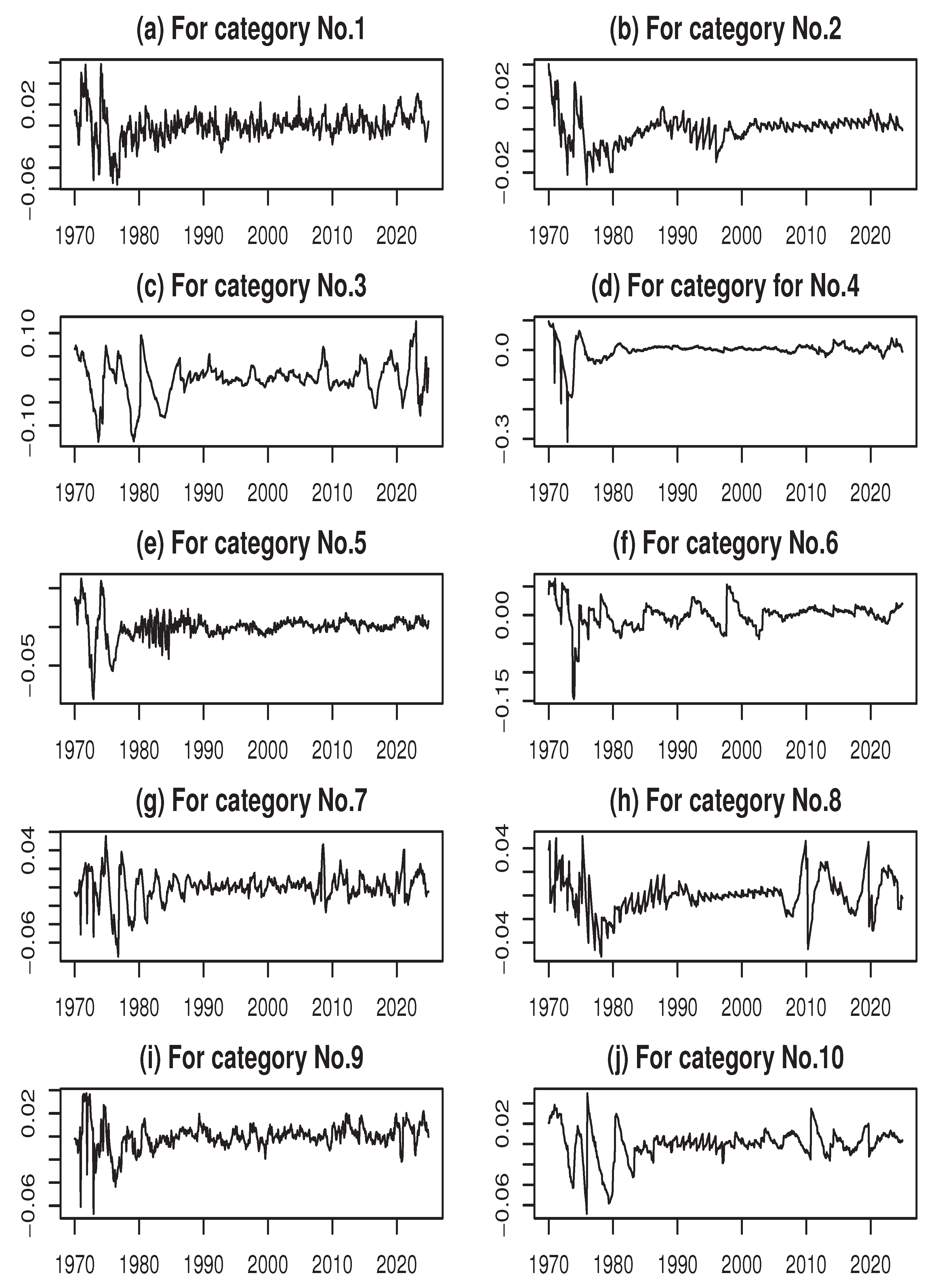
As outlined in Section 2.1, the cyclical component of each CPI category in Table 1 is treated as a distinct variable. Data of all variables can be obtained from the website of the Statistics Bureau of Japan (https://www.stat.go.jp/english/data/cpi/1581-z.html), with historical series linked to maintain continuity across changes in 2020 base CPI. The dataset consists of monthly observations covering the period from January 1970 to December 2024, as reported in Kyo and Noda (2025b). A visual summary of the time series for all ten variables is provided in Figure A1 in Appendix.
3.2. Analyzing the Common Factor
The maximum lag length is set to 12, so that for each variable the lag parameters are estimated within the range of to 12. The resulting estimates will be examined in detail in the next subsection.
Figure 1(a) displays the estimated common factor, while Figure 1(b) shows the standardized cyclical component of the overall CPI for comparison.
Figure 1.
Estimated common factor (a) and standardized cyclical component of the overall CPI (b). Shaded areas correspond to the Japanese business cycle dates by the Economic and Social Research Institute, which is a think tank within the Cabinet Office of the Japanese government.
Figure 1.
Estimated common factor (a) and standardized cyclical component of the overall CPI (b). Shaded areas correspond to the Japanese business cycle dates by the Economic and Social Research Institute, which is a think tank within the Cabinet Office of the Japanese government.
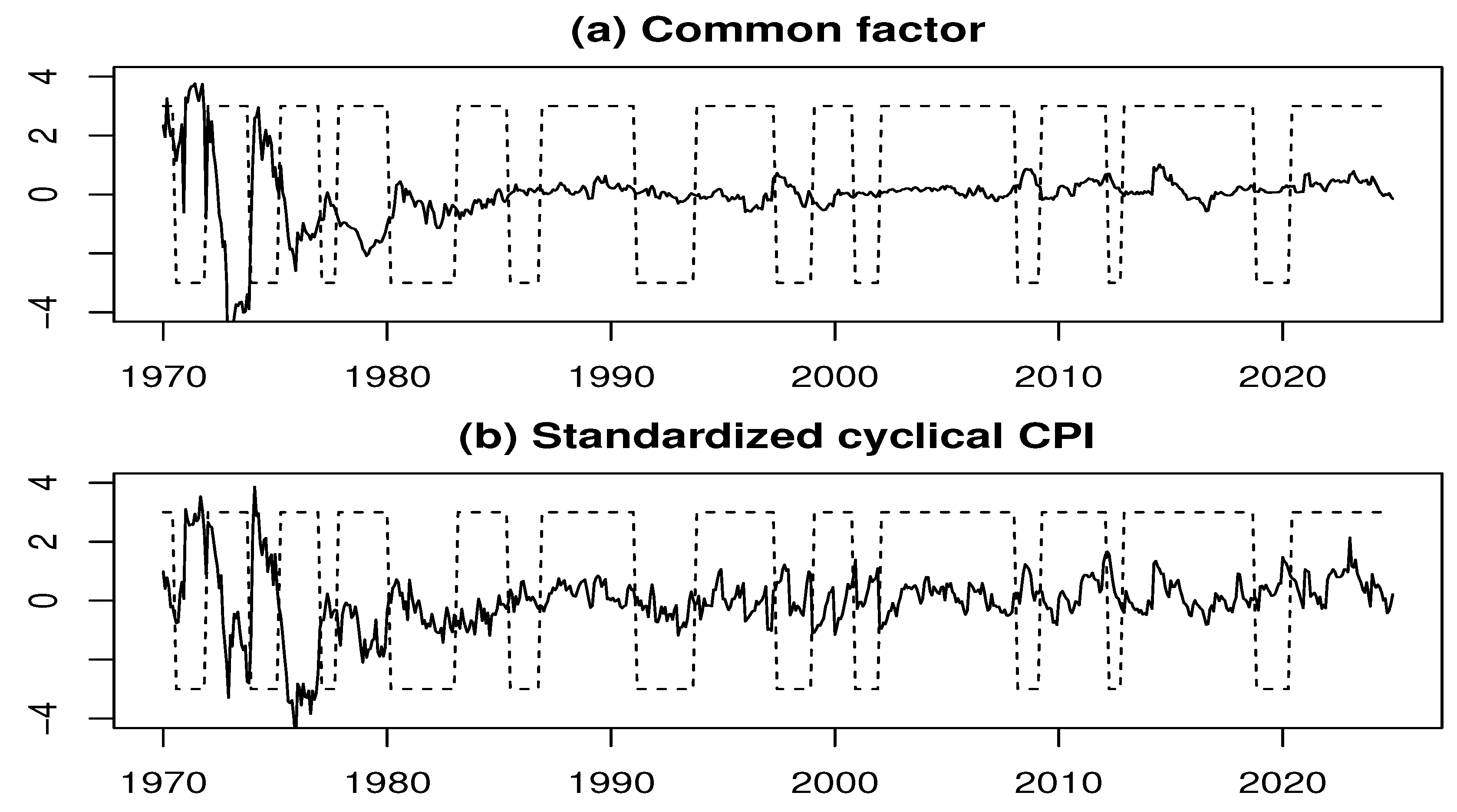
From Figure 1(a) and Figure 1(b), we find that both series exhibit pronounced fluctuations until the mid-1970s, after which the amplitude of variation gradually decreases. Moreover, the cyclical component of the overall CPI features numerous irregular peaks and troughs, whereas the estimated common factor remains comparatively stable. Furthermore, the common factor tends to decline during recession periods, reflecting the impact of macroeconomic downturns on category-level price dynamics.
Using Equation (2), the CPFI can be directly constructed from the estimated common factor. As this involves only a linear scale transformation, the corresponding figure is omitted.
3.3. Lead–Lag Relationships between CPI Categories and the Common Factor
Table 2 reports the estimated lags for the ten CPI categories.
These estimates allow each category to be classified into one of the six groups defined in Section 2.3.2, clarifying their roles in leading or responding to common cyclical fluctuations. The raw estimates reveal diverse lead–lag patterns. For example, Food (No.1) with the lags and Fuel, Light and Water Charges (No.3) with the lags belong to the co-varying and outcome group, indicating that these essential goods generally move with the common cycle but respond with delays due to factors such as import prices, energy shocks, or supply constraints. Clothes and Footwear (No.5) with the lags serves in the role of a clear causal driver, leading overall CPI fluctuations.
Housing (No.2) with the lags , Culture and Recreation (No.9) with the lags , and Miscellaneous (No.10) with the lags are bipolar categories, exhibiting both leading and lagging behavior depending on historical context. These categories reflect structural heterogeneity and context-dependent responses to macroeconomic shocks.
Medical Care (No.6) with the lags and Education (No.8) with the lags are outcome categories with long lags, highlighting structural rigidity and regulatory constraints. Furniture and Household Utensils (No.4) with the lags and Transportation and Communication (No.7) with the lags primarily follow the common cycle, adjusting after shocks propagate through the macroeconomy.
To emphasize broader patterns, categories are aggregated by group as summarized in Table 3.
As Table 3 demonstrates, Japan’s CPI categories exhibit substantial heterogeneity in their interactions with the common factor. Causal categories, such as Clothes and Footwear, serve as early indicators of broader price movements, providing potential signals for policy monitoring. Most categories fall into outcome or co-varying and outcome groups, highlighting the reactive nature of category-level CPI to common shocks. Bipolar categories illustrate that lead–lag relationships vary across historical episodes, reflecting structural and institutional features of the Japanese economy.
A primary goal of monetary policy is usually considered to be price stability (Ito and Hoshi, 2020, Ch.6). From a policy perspective, monitoring sector-specific dynamics can enhance the timeliness and effectiveness of stabilization measures. Causal categories may function as early-warning indicators of inflationary pressures, while outcome categories reflect lagged adjustments that policymakers of central banks must address. Bipolar categories underscore the context-dependent nature of cyclical responses and structural heterogeneity in the macroeconomy.
3.4. Analyzing the Dynamics of Relationships Between the Variables and the Common Factor
In this subsection, we present the estimated time-varying factor loadings (TVFLs) and examine the dynamic relationships between each variable and the common factor. Both the variables and the common factor are centered and standardized, so that each TVFL represents the time-varying correlation coefficient between a variable and the common factor at the corresponding lag.
Figure 2.
Time series of the TVFLs for variables Nos. 1 to 3.
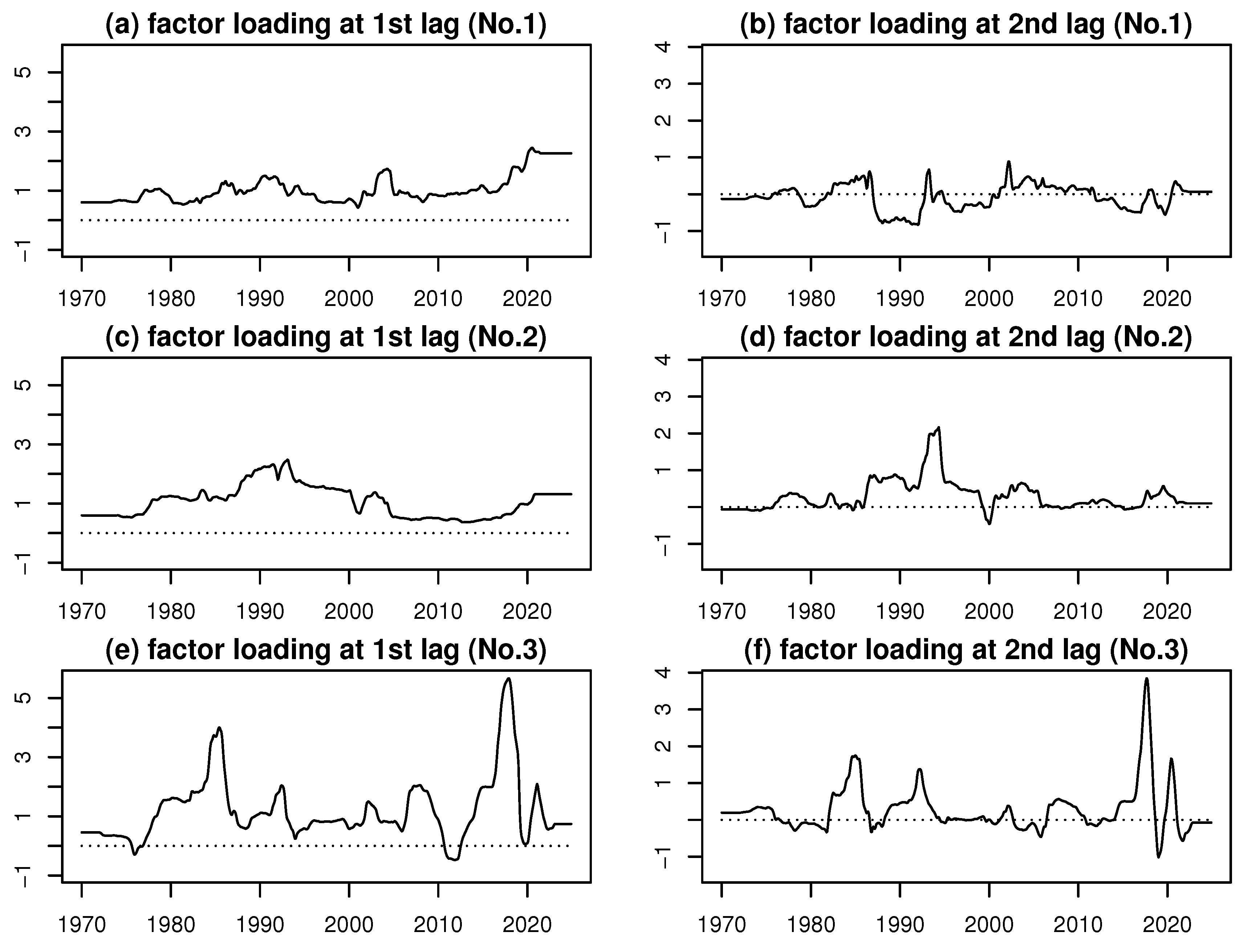
Figure 3.
Time series of the TVFLs for variables Nos. 4, 6, and 7.
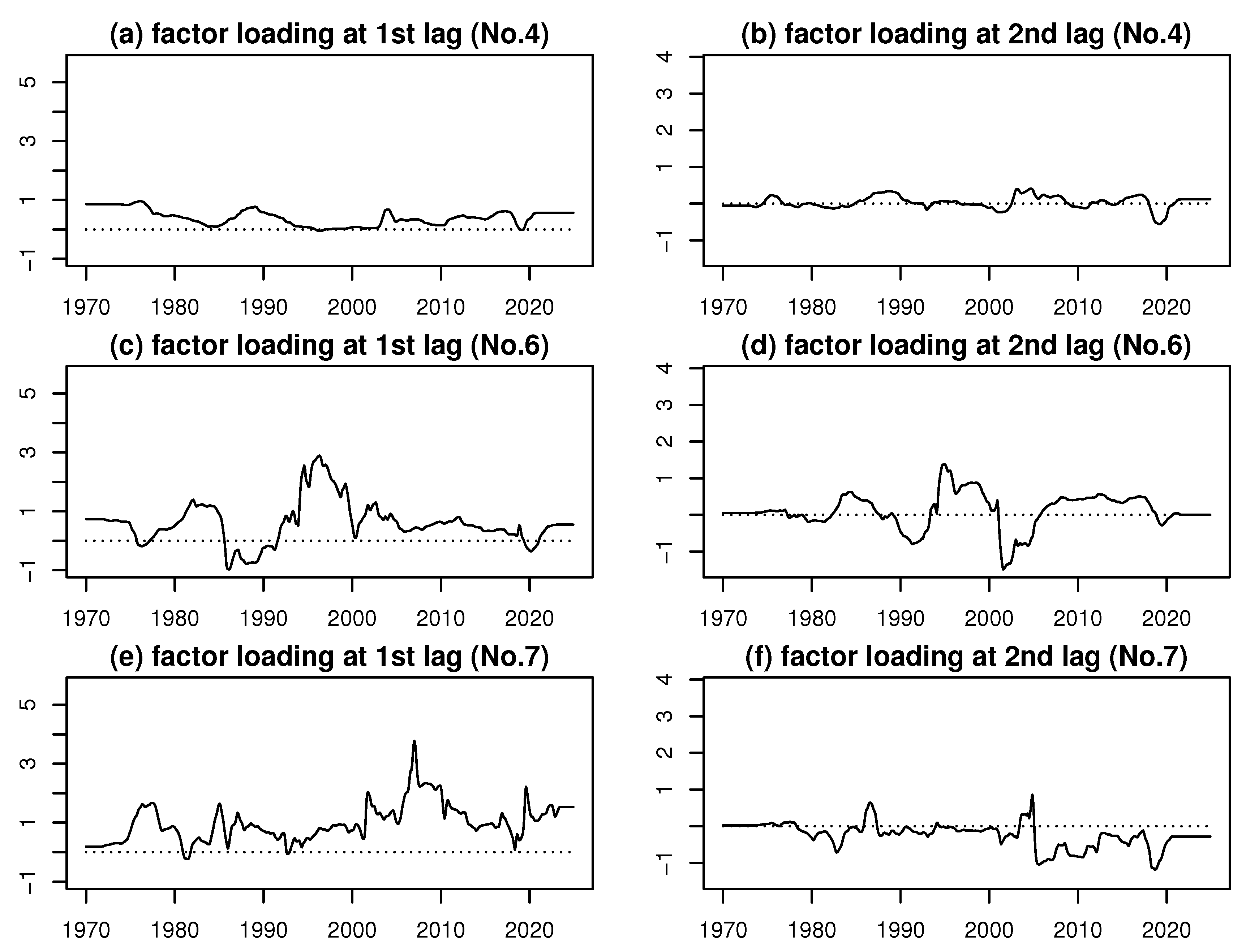
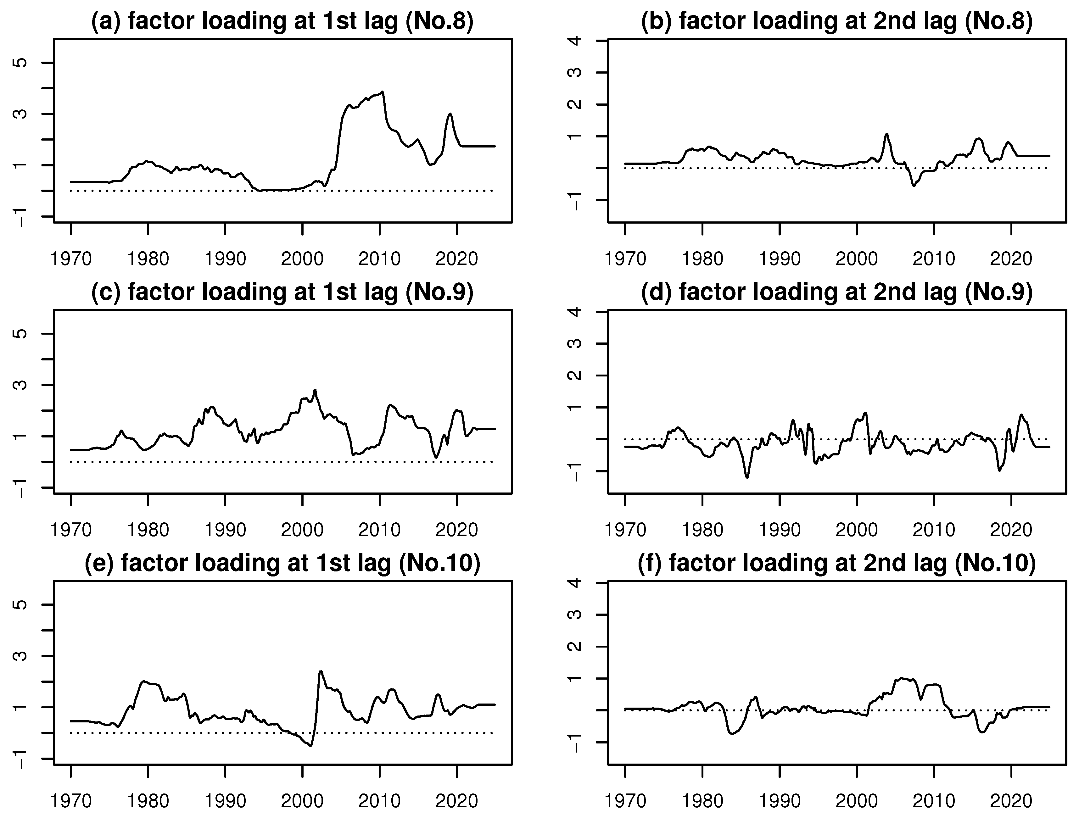
Figure 4.
Time series of the TVFLs for variables Nos. 8 to 10.
Regarding variable No. 5, because the two estimated lags are equal, the corresponding TVFLs are combined into a single combined factor loading (CFL), shown in Figure 5.
This CFL provides a concise representation of the overall dynamic relationship between variable No. 5 and the common factor.
Food (No. 1)
The first-lag TVFL (Figure 2(a)) remains nearly constant at 0.6 in the early 1970s, indicating a weak but stable correlation. It gradually increases from 1973, reaching around 1.0 by the late 1970s, reflecting a strengthening association after the first oil crisis (1973–1974). During the 1980s to early 1990s, the loading peaks above 1.2 before stabilizing between 0.8 and 1.0. From the 2000s, the TVFL rises sharply, exceeding 2.0 in the mid-2000s and stabilizing at 2.26 toward the end of the sample, suggesting a persistently strong link with the common factor.
The second-lag TVFL (Figure 2(b)) exhibits more volatile dynamics. It starts at in the early 1970s, rises toward zero by the late 1970s, and alternates between positive and negative values throughout the 1980s–2000s. Toward the end of the sample, it stabilizes around 0.07, indicating a weak but positive delayed correlation. Overall, the first-lag effect dominates over time, while the second-lag effect loses explanatory power.
Housing (No. 2)
The first-lag TVFL (Figure 2(c)) begins near 0.6 and remains stable in the early 1970s. A gradual increase begins in the mid-1970s, reaching above 2.0 by 1990, followed by corrections and eventual stabilization around 1.3 by 2008. These dynamics reflect increasing sensitivity to the common factor over time, possibly due to structural changes or policy shifts.
The second-lag TVFL (Figure 2(d)) starts near , indicating a weak negative correlation. It rises steadily from the late 1970s, peaks around 2.0 in early 1993, and then declines to stabilize around 0.10. This trajectory illustrates a transition from weak negative association to strong positive alignment and finally to moderate correlation, highlighting structural changes in the relationship.
Fuel, Light and Water Charges (No. 3)
The first-lag TVFL (Figure 2(e)) shows how short-term energy price shocks are transmitted to the common factor, indicating that this category primarily co-varies with but slightly lags overall CPI fluctuations. The second-lag TVFL (Figure 2(f)) captures more persistent cost-push effects stemming from imported fuel and utilities, highlighting delayed yet sustained contributions to cyclical price movements.”
Furniture and Household Utensils (No. 4)
The first-lag TVFL (Figure 3(a)) reflects immediate adjustments to household spending cycles, while the second-lag TVFL (Figure 3(b)) reveals slower inventory and replacement effects. Together they suggest that this category follows the common cycle with modest delays but can amplify turning points during periods of rapid demand change.
Medical Care (No. 6)
The first-lag TVFL (Figure 3(c)) begins at 0.74 and gradually decreases, turning negative around 1974–1986, reflecting temporary reversal. It peaks at approximately 2.7 between 1986 and 1994 and later stabilizes around 0.55 – 0.8.
The second-lag TVFL (Figure 3(d)) starts near 0.05, rises gradually to 0.5, peaks above 1.0 in the period from 1983 to 2001, and eventually declines toward zero. These patterns indicate that the first-lag effect captures the dominant long-term alignment, while the second-lag effect reflects transient structural deviations.
Transportation and Communication (No. 7)
The first-lag TVFL (Figure 3(e)) indicates that transportation and communication prices tend to move contemporaneously with the common factor, reflecting their sensitivity to fuel costs and general demand conditions. The second-lag TVFL (Figure 3(f)) points to lingering effects from regulatory adjustments and contract renewals, implying a gradual transmission of shocks across subcomponents.
Education (No. 8)
The first-lag TVFL (Figure 4(a)) remains stable near 0.35 until early 1973, then rises steadily, reaching about 1.16 by the late 1970s. It fluctuates moderately during 1981–1989, declines to near zero by 1994, and exhibits a sharp rise between 1999 and 2009, surpassing 3.7. After a gradual decline, a second peak occurs around 2019, followed by stabilization at 1.74.
The second-lag TVFL (Figure 4(b)) starts at 0.14, gradually rises to 0.6 in the mid-1970s, and fluctuates until mid-1990s. It then experiences a period, 2001–2004, of strong influence, followed by a temporary negative phase () around 2006–2009 and final stabilization around 0.38. These dynamics show that the first-lag effect dominates long-term behavior, while the second-lag effect captures temporary and occasionally inverse relationships.
Culture and Recreation (No. 9)
The first-lag TVFL (Figure 4(c)) reveals episodes when discretionary spending in culture and recreation leads or coincides with the common factor, acting as an early signal of changing household sentiment. The second-lag TVFL (Figure 4(d)), in contrast, captures delayed responses during downturns when households postpone non-essential consumption, producing oscillatory patterns.
Miscellaneous (No. 10)
The first-lag TVFL (Figure 4(e)) shows a weak but variable contemporaneous link to the common factor, reflecting the diverse nature of this category. The second-lag TVFL (Figure 4(f)) uncovers protracted and sometimes opposing effects from heterogeneous subitems, underscoring the importance of disaggregated analysis for accurate policy interpretation.
Combined Factor Loading (Variable No. 5)
For Clothes and Footwear (No. 5), the two lags coincide, yielding a combined factor loading (CFL, Figure 5). The CFL captures the overall dependence on the common factor, exhibiting long-term stability with moderate fluctuations, highlighting consistent influence on the CPFI.
Summary
Across the examined variables, first-lag TVFLs generally reflect the dominant, long-term alignment with the common factor, while second-lag TVFLs capture transient, oscillatory, or occasionally opposing effects. These dynamics reveal that the contemporaneous impact of the common factor often strengthens over time, whereas delayed effects are less consistent. Structural changes, policy shifts, and exogenous shocks contribute to the observed temporal evolution of these relationships.
3.5. Analyzing the Interaction Between the Variables and the Common Factor
Even within the same variable, its relationship with the common factor can be intricate and time-varying. For instance, one lag may load negatively, indicating that the variable leads fluctuations in the common factor, while another lag may load positively, reflecting a delayed response. Variable No. 2 exemplifies this pattern, with the first lag negative and the second lag positive. These contrasting signs and magnitudes illustrate how the two TVFLs capture complex and multi-layered interactions. This feature distinguishes the TLTVFL model from static factor-loading approaches.
Figure 6 depicts a scatter plot with line graphs showing the simultaneous evolution of the first- and second-lag TVFLs for variable No. 2.
To emphasize underlying patterns, the TVFL time series are smoothed using the MLM approach. In Figure 6, the first-lag TVFL is plotted on the horizontal axis, representing the variable’s leading influence on the common factor, while the second-lag TVFL is plotted on the vertical axis, representing its delayed response. These TVFLs reflect the link between the variable and the common factor through the latter, which acts as a latent intermediary summarizing overall price dynamics.
Several observations can be made from Figure 6.
- Early stage (before 1975): Both TVFLs are small and negative (around –0.05 to –0.06). The joint movement indicates that variable No. 2 was initially weakly but stably negatively aligned with the common factor, with nearly equal contributions from both lags.
- Transition phase (end of 1974 to mid-1986): The second-lag TVFL rises and turns positive, while the first-lag TVFL also trends upward but with smaller amplitude. This divergence implies that the second lag increasingly dominates the explanatory power.
- Peak synchronization phase (mid-1986 to early 1993): The second-lag TVFL surges to nearly 2.0, whereas the first-lag TVFL rises modestly. Variable No. 2 becomes strongly synchronized with the common factor, dominated by the second-lag effect.
- Late stage (after early 1993): Both TVFLs decline and stabilize at weak positive levels (around 0.1), suggesting that variable No. 2 gradually decouples from the common factor.
Overall, the joint dynamics of the two TVFLs reveal regime shifts in the role of variable No. 2. Initially balanced at weak negative levels, subsequently dominated by the second lag, and finally reconverging to weak, stable positive values. These patterns reflect structural changes in the underlying system, highlighting the TLTVFL model’s ability to uncover hidden asymmetries and time-varying dependencies not detectable by static factor loadings. In practical terms, this implies that housing prices not only drive overall price fluctuations but also tend to move broadly in the same direction as the general price level.
The analysis above focused on a variable with contrasting negative and positive lags. Naturally, analogous investigations can be applied to other lag patterns to reveal complex and time-varying interactions with the common factor.
4. Concluding Remarks
This study applied the Time-Lagged Two-Variable Factor Loading (TLTVFL) model to the cyclical components of ten major CPI categories in Japan, covering the period from January 1970 to December 2024. The primary objective was to elucidate the dynamic interactions between individual CPI categories and the common factor driving overall price fluctuations, while explicitly accounting for time-varying relationships. By integrating estimated lag structures with time-varying factor loadings (TVFLs), our approach identified contemporaneous and delayed effects, leading and lagging roles, and complex interdependencies across categories.
Our analytical results revealed substantial heterogeneity among CPI categories. Clothes and Footwear (No. 5) consistently acted as a causal driver, leading overall CPI movements. In contrast, Medical Care (No. 6) and Education (No. 8) primarily served as outcome categories, responding with long lags due to regulatory and structural constraints. Essential goods and services such as Food (No. 1) and Fuel, Light and Water Charges (No. 3) co-varied with the common factor but exhibited delayed responses indicative of cost-push influences. Housing (No. 2), Culture and Recreation (No. 9), and Miscellaneous (No. 10) behaved as bipolar categories, displaying both leading and lagging tendencies depending on historical periods, thereby highlighting the structural heterogeneity and context-dependent nature of their cyclical responses.
Time-varying factor loadings provided a detailed view of how each variable’s relationship with the common factor evolved over time. First-lag TVFLs generally exhibited persistent trends, reflecting the strengthening of contemporaneous relationships, whereas second-lag TVFLs oscillated, capturing delayed and occasionally opposing effects. For example, Food (No. 1) displayed a steadily increasing first-lag TVFL, indicating a growing alignment with the common factor over the decades, while the second-lag TVFL fluctuated substantially, reflecting unstable delayed responses. Housing (No. 2) exhibited distinct phases—initial weak negative alignment, an intermediate period dominated by the second lag, and eventual stabilization at weak positive levels. These dynamics likely reflect structural shifts and regime changes in the Japanese economy.
The TLTVFL model offers clear methodological advantages over conventional static factor models. By allowing factor loadings to vary over time and incorporating multiple lags, it captures asymmetric, non-stationary, and regime-dependent relationships that static approaches cannot detect. The use of combined factor loadings (CFLs) for equal lags provides a concise yet informative summary of overall dependence on the common factor, thereby enhancing interpretability. Furthermore, classifying CPI categories into causal, outcome, co-varying, and bipolar groups enables systematic insights into sector-specific dynamics.
From a policy perspective, these findings emphasize the importance of monitoring sector-specific price dynamics. Causal categories may serve as early-warning indicators of emerging inflationary pressures, while outcome categories illustrate the delayed transmission of shocks, underscoring the need for forward-looking policy interventions. Bipolar categories demonstrate that the effects of macroeconomic shocks are neither uniform nor constant over time, highlighting the necessity of flexible and context-sensitive policy measures. Continuous tracking of TVFLs can also reveal emerging structural shifts or changes in cyclical sensitivities, enabling more effective policy responses.
As demonstrated in previous sections, Japan’s CPI dynamics are characterized by pronounced heterogeneity, evolving correlations, and structural shifts across categories. The TLTVFL modeling approach effectively captures these complex interactions, offering a novel analytical tool and valuable insights into the mechanisms underlying business cycles. Thus, our framework deepens the understanding of inflation dynamics and contributes to evidence-based policymaking for price stabilization. Moreover, the findings lay the groundwork for future research, including applications to other macroeconomic indicators, high-frequency datasets, and cross-country comparisons.
Acknowledgments
This work was supported in part by a Grant-in-Aid for Scientific Research (C) (20K01639) from the Japan Society for the Promotion of Science.
Conflicts of Interest
The authors declare that there are no conflicts of interest regarding the publication of this article.
Appendix A. Figures for the Variables
Figure A1.
Time series of the cyclical components used as variables in the analysis.
References
- Baxter, M. and King, R. (1999), “Measuring business cycles: Approximate band-pass filter for economic time series,” The Review of Economics and Statistics, 81(4), pp. 575-593. [CrossRef]
- Blinder, A. S. (1982), “Inventories and sticky prices: More on the microfoundations of macroeconomics,” American Economic Review, 72(3), pp. 334-348.
- Boskin, M. J., Dulberger, E. L., Gordon, R. J., Griliches, Z., and Jorgenson, D. W. (1998), “Consumer prices, the consumer price index, and the cost of living,” Journal of Economic Perspectives, 12(1), pp. 3-26. [CrossRef]
- Bryan, M. F. and Cecchetti, S. G. (1993), “The consumer price index as a measure of inflation,” Federal Reserve Bank of Clevel, Economic Review, 29(4), pp. 15-24.
- Hale, G. and Jordà, Ò. (2007), “Do monetary aggregates help forecast inflation?,” FRBSF Economic Letter, 2007-10, pp. 1-4.
- Harvey, A. C. (1990), Forecasting, Structural Time Series Models and the Kalman Filter, Cambridge: Cambridge University Press.
- Ito, T. and Hoshi, T. (2020), The Japanese Economy, 2nd Edition, Cambridge: The MIT Press.
- Kyo, K. (2025), “Reinforcing moving linear model approach: Theoretical assessment of parameter estimation and outlier detection,” Axioms, 14(7), 479, pp. 1-26. [CrossRef]
- Kyo, K. and Kitagawa, G. (2023), “A moving linear model approach for extracting cyclical variation from time series data,” Journal of Business Cycle Research, 19(3), pp. 373-397. [CrossRef]
- Kyo, K. and Noda, H. (2025a), “Analyzing mechanisms of business fluctuations involving time-varying structure in Japan: Methodological proposition and empirical study,” Computational Economics, Published Online, pp. 1-60. [CrossRef]
- Kyo, K. and Noda, H. (2025b), “Analyzing the structural dynamics of Japan’s consumer prices: A component decomposition approach,” Preprints.org. [CrossRef]
- Kyo, K. and Noda, H. (2025c), “Unveiling the dynamics of wholesale commercial sales and business cycle impacts in Japan: An extended moving linear model approach,” Preprints.org. [CrossRef]
- Kyo, K., Noda, H., and Fang, F. (2024), “An integrated approach for decomposing time series data into trend, cycle and seasonal components,” Mathematical and Computer Modelling of Dynamical Systems, 30(1), pp. 792-813. [CrossRef]
- Stock, J. H. and Watson, M. W. (1989), “New indexes of coincident and leading macroeconomic indicators,” In: O. Blanchard and S. Fischer (eds.), NBER Macroeconomics Annual, pp. 351-394. Cambridge: The MIT Press.
- Stock, J. H. and Watson, M. W. (1991), “A probability model of the coincident economic indicators,” In: K. Lahiri and G. Moore (eds.), Leading Economic Indicators: New Approaches and Forecasting Records, pp. 63-89, Cambridge: Cambridge University Press.
- Stock, J. H. and Watson, M. W. (2009), “Forecasting in dynamic factor models subject to structural instability,” In: J. Castle and N. Shephard (eds.), The Methodology and Practice of Econometrics, A Festschrift in Honour of Professor David F. Hendry, pp. 1-57, Oxford: Oxford University Press.
- Stock, J. H. and Watson, M. W. (2016), “Dynamic factor models, factor-augmented vector autoregressions, and structural vector autoregressions in macroeconomics,” Handbook of Macroeconomics, 2A, pp. 415-525. Amsterdam: Elsevier. [CrossRef]
- Su, L. and Wang, X. (2017), “On time-varying factor models: Estimation and testing,” Journal of Econometrics, 198(1), pp. 84-101. [CrossRef]
Figure 5.
Time series of the combined factor loading (CFL) for variable No. 5.
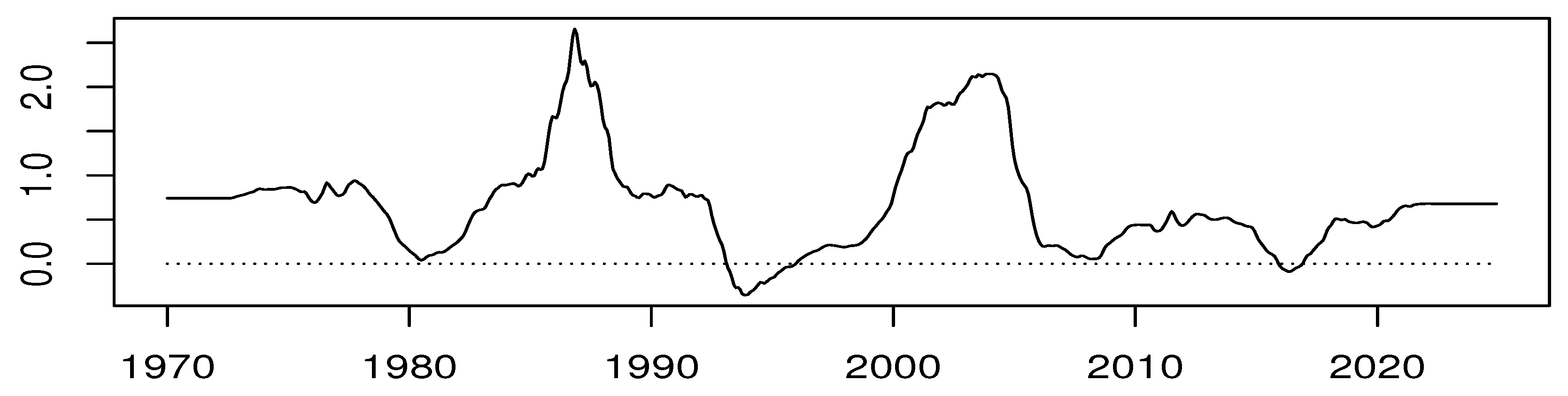
Figure 6.
Scatter plot of TVFLs at the second and first lags for variable No. 2 (red and blue dots denote start and end points, respectively; arrows indicate time direction).
Figure 6.
Scatter plot of TVFLs at the second and first lags for variable No. 2 (red and blue dots denote start and end points, respectively; arrows indicate time direction).
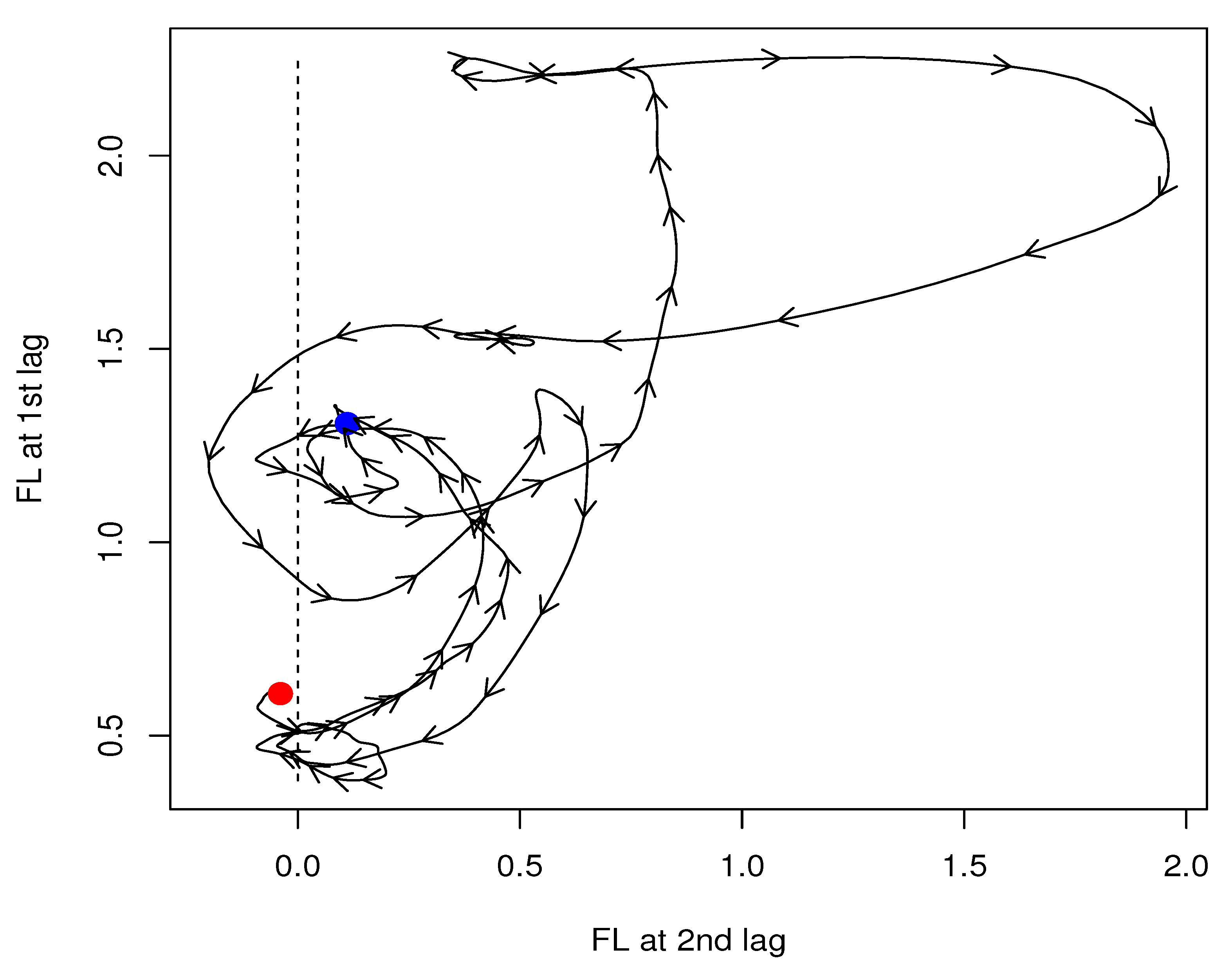

Table 1.
Major Categories of the CPI in Japan.
| No. | Category |
|---|---|
| 1 | Food |
| 2 | Housing |
| 3 | Fuel, Light and Water Charges |
| 4 | Furniture and Household Utensils |
| 5 | Clothes and Footwear |
| 6 | Medical Care |
| 7 | Transportation and Communication |
| 8 | Education |
| 9 | Culture and Recreation |
| 10 | Miscellaneous |
Table 2.
Estimated Lags for Each CPI Category.
| Variable No. | 1 | 2 | 3 | 4 | 5 | 6 | 7 | 8 | 9 | 10 |
|---|---|---|---|---|---|---|---|---|---|---|
| Estimate for | 0 | 0 | 0 | 11 | 0 | 12 | 0 | 1 | ||
| Estimate for | 4 | 1 | 6 | 2 | 1 | 3 | 0 |
Table 3.
CPI Categories Classified by Lead–Lag Group.
| Group | Categories | Interpretation | |
|---|---|---|---|
| Causal | Clothes and Footwear (No.5) | (,) | Leads overall CPI; anticipates broader price movements driven by seasonal cycles and import costs. |
| Outcome | Medical Care (No.6), Education (No.8) | (11,1), (12,0) | Respond slowly due to regulatory and structural rigidity; long lags indicate limited short-term responsiveness. |
| Co-varying and Outcome | Food (No.1), Fuel, Light and Water Charges (No.3), Furniture and Household Utensils (No.4), Transportation & Communication (No.7) | (0,2), (0,3) | Move with the common cycle but exhibit delayed responses, reflecting cost-push effects, energy price shocks, or short-term adjustment dynamics. |
| Bipolar | Housing (No.2), Culture & Recreation (No.9), Miscellaneous (No.10) | (,1), (0,), (1,) | Exhibit both leading and lagging behavior depending on subcomponents or historical context; highlight structural heterogeneity and context-dependent cyclical responses. |
Disclaimer/Publisher’s Note: The statements, opinions and data contained in all publications are solely those of the individual author(s) and contributor(s) and not of MDPI and/or the editor(s). MDPI and/or the editor(s) disclaim responsibility for any injury to people or property resulting from any ideas, methods, instructions or products referred to in the content. |
© 2025 by the authors. Licensee MDPI, Basel, Switzerland. This article is an open access article distributed under the terms and conditions of the Creative Commons Attribution (CC BY) license (https://creativecommons.org/licenses/by/4.0/).
Copyright: This open access article is published under a Creative Commons CC BY 4.0 license, which permit the free download, distribution, and reuse, provided that the author and preprint are cited in any reuse.


