Submitted:
04 August 2025
Posted:
07 August 2025
You are already at the latest version
Abstract
Wholesale sales value is one of the key elements included in the coincident indicator series of the indexes of business conditions in Japan. The objectives of this study are twofold. The first is to comprehend features of dynamic structure of various components for 12 business types of the wholesale commercial sales in Japan, focusing on the period from January 1980 to December 2022. The second is to elucidate effect of business cycles on the behavior of each business type of the wholesale commercial sales. Specifically, we utilize our moving linear model approach to decompose monthly time series data of wholesale commercial sales into a seasonal component, an unusually varying component containing outliers, a constrained component, and a remaining component. Additionally, we construct a distribution-free dynamic linear model and examine the time-varying relationship between the decomposed remaining component, which contains cyclical variation, in each business type of the wholesale commercial sales and that in the coincident composite index. Our proposed approach reveals complex dynamics of various components of time series on wholesale commercial sales. Furthermore, we find that different business types of the wholesale commercial sales exhibit diverse responses to business cycles, influenced by macroeconomic conditions, government policies, or exogenous shocks.
Keywords:
component decomposition
; economic time series
; dynamic structure
; Japanese economy
; moving linear model approach
; wholesale commercial sales
1. Introduction
Wholesale sales value is one of the key elements included in the coincident indicaor series of the indexes of business conditions in Japan. However, despite a common recognition of the importance of wholesale commercial sales, there have been no studies on the detailed examination of components of time series data on various business types of the wholesale commercial sales, which leads to elucidation of features of dynamic structure in wholesale commercial sales sectors. Another important unresolved issue is the relationship between the various types of wholesale commercial sales and the business cycles. These issues are crucial in deepening our understanding of the significance of including wholesale sales value in the indexes of business conditions.
Although there are numerous instances of data analysis in various socio-economic fields, comparable cases of data analysis within the same field are not commonly observed, with different methods being employed in each instance. For example, Wang (2017) conducted an analysis of the impact of sudden events on China’s automobile industry stock prices using the incident research method. Noda and Kyo (2019) examined the validity of including wholesale and retail commercial sales in the coincident indexes of business conditions in Japan. Gupta et al. (2023) analyzed the evolution of the retail sector during the coronavirus disease 2019 (COVID-19) using the Scopus bibliographic database and identified future research issues.
From a methodological perspective on time-series analysis, various approaches have been proposed. Box et al. (2008) provide a foundation of time series analysis, forecasting methods, and control techniques. Brockwell and Davis (1991) introduced basic theories and methods for time series analysis, while Brockwell and Davis (2016) serve as a comprehensive guide, introducing readers to modeling techniques used in analyzing sequential data. These references fall within the scope of traditional time series analysis, primarily dealing with stationary time series. For non-stationary time series, such as those with mean non-stationarity, it is common to take differences to approximately transform the original time series into a stationary form before applying conventional methods. However, there is a drawback in processing time series through differencing, as it leads to a loss of information contained in the original data. Therefore, methods have been proposed to decompose the original time series into several components, separating stationary and non-stationary components (see, e.g., Kitagawa and Gersch, 1984; Kitagwa, 2020). Moreover, Kitagawa and Gersch (1985) introduced a method of autoregressive modeling with time-varying coefficients to analyze autocorrelation non-stationary time series. Adeosun et al. (2023) analyzed the dynamics of oil and food prices using the bootstrapped time-varying Granger causality method by Shi et al. (2020) to identify and examined date-stamp causal changes in the predictive effects between oil and food markets. Note that Kitagawa-Gersch’s approaches may not function effectively depending on the nature of the data. For instance, Kitagawa and Gersch (1984) sometimes face challenges in successfully separating cyclical components (see, e.g., Kyo et al., 2022). Furthermore, existing approaches often rely on strict assumptions about the distribution of the data, such as normality, homoscedasticity and heteroscedasticity assumptions. To address these issues, Kyo and Kitagawa (2023) proposed the moving linear model approach. The distinctive feature of this approach lies in its simplicity and flexibility in modeling, eliminating the need for stringent assumptions about the data distribution.
We consider the monthly time series data of wholesale commercial sales to be composed of a seasonal component, an unusually varying component containing outliers (representing abnormal variations), a constrained component (representing the trend), and a remaining component (representing cyclical variations). Thus, the purpose of this research is the following two points. The first is to comprehend dynamic features of various components for 12 business types of the wholesale commercial sales in Japan. Specifically, 12 business types of the wholesale commercial sales are as follows: General Merchandise, Textiles, Apparel and Accessories, Livestock and Aquatic Products, Food and Beverages, Building Materials, Chemicals, Minerals and Metals, Machinery and Equipment, Furniture and House Furnishings, Medicines and Toiletries, and Others. The second is to elucidate effects of business fluctuations on the behavior of each business type of the wholesale commercial sales. The significance of wholesale commercial sales extends beyond economic indicators, providing insights into global movements, societal shifts, and the repercussions of unforeseen events such as economic downturns or natural disasters. The analysis of these sales offers a multifaceted perspective. Therefore, we target the wholesale sector to elucidate structural changes in 12 business types of the wholesale commercial sales over time and discern influences of business fluctuations on the behavior of each business type of the wholesale commercial sales.
To achieve the first objective, we employ the moving linear model approach developed by Kyo and Kitagawa (2023). In addition, we conduct the anomaly detection and estimation using the method proposed by Kyo (2025). These methodologies aid in decomposing each time series into trend, seasonal variation, cyclical patterns, and abrupt fluctuations, allowing for an in-depth investigation into the factors and outcomes influencing each component’s variations. Regarding the second objective, we analyze effects of business fluctuations using the coincident composite index (CI) as an index for business cycle analysis. This involves exploring the relationship between the coincident CI and the cyclical components in wholesale commercial sales of every business type. While recognizing the temporal variability of such relationships, we address this challenge by employing a time-varying coefficient linear model. It should be noted that given the complexity of the error term’s probability distribution in such linear models, conventional modeling approaches become challenging. Thus, we propose a novel approach based on the moving linear model by Kyo and Kitagawa (2023) and apply to analyze the dynamic relationships in the second objective, establishing the framework of this study. Our analytical results reveal the complex dynamics of the various components of the time series on commercial wholesale sales. Additionally, each business type of commercial wholesale sales value responds diversely to business fluctuations, influencing exogenous and serious shocks, such as the global financial crisis and the COVID-19 pandemic.
The remainder of this article is organized as follows. In Section 2, we provide a detailed review of our previous research, including the moving linear model approach and its extended version. Section 3 presents an illustrative example for decomposing time series for wholesale commercial sales of each business type in Japan and analyzing the dynamics in the decomposed results. In Section 4, we newly introduce a time-varying linear model approach for analyzing the dynamics in the relationship between the cyclical components in wholesale commercial sales of every business type and business fluctuations. Section 5 presents another illustrative example by applying the approach introduced in Section 4. In Section 6, we present a summary and discussion.
2. Detailed Review of Our Previous Research
2.1. Moving Linear Model Approach
As a fundamental cornerstone for the present study, in this section we offer a comprehensive review of the moving linear model approach proposed by Kyo and Kitagawa (2023), and its extended versions introduced by Kyo et al. (2024) and Kyo (2025).
2.1.1. Basic Model
Consider that decompose a time series into two unobserved components as follows:
with and denoting the constrained and remaining components, respectively, where t represents a specific time point, and N is the sample size. The constrained component reflects long-term variation, expected to be highly smoothed, while the remaining component captures short-term variation, it often represents cyclical fluctuations in the time series . To ensure a unique decomposition, the average of the remaining component over a given data span is assumed to be zero.
To achieve smoothness for the constrained component, a linear model of time t is introduced as follows:
where k is an integer which represents the width of the time interval for , and and are the coefficients. When a centered time variable within the n-th time interval is introduced as:
In Equation (3), represents the midpoint of the time interval. So, by substituting the model in Equation (2) is rewritten as:
where . The model in Equation (1) is then expressed as
or in vector form of Equation (4) as follows:
In Equation (5),
and denotes a k-dimensional vector in which all elements are 1.
Furthermore, we set
denoting the vector associated with the remaining component for in the -th time interval. It can be observed that and represent the same term, namely , of the remaining component for . However, they may undergo slight changes to accommodate for and in the -th and n-th time intervals. Thus, for a given value of n, the following relationship holds:
where represents the variation between and .
The model introduced above is referred to as the moving linear model, and the approach based on this model is called the moving linear model approach.
2.1.2. Estimation of Remaining Component
In Equation (6), the quantities , and are treated as the parameters. To achieve stable parameter estimates, a Bayesian approach was adopted.
First, it was assumed that and exhibit smooth variations with respect to n as
under diffuse priors for and . That is, we assume that and in Equation (7), where the variance can be set to a sufficiently large value.
Furthermore, to obtain stable estimates for the remaining component it is assumed that is orthogonal to and . Thus, the following equation is introduced:
Applying Equation (6) to the relations in Equation (8), we set
Here, Equation (9) represents the priors for and . Moreover, the priors for are established as follows:
In Equation (10), represent a set of system noises. It was assumed that and are independent for , where is regarded as an unknown parameter.
Moreover, under the settings
with denoting a k-dimensional unit matrix, a set of Bayesian model for the moving linear model can be expressed by a state-space form as
with , where . Here, , and in Equations (13) and (14) are defined in Equations (11) and (12).
Thus, given the initial conditions and , and the observations , we can obtain the mean vectors and the covariance matrices of the state for using the following Kalman filter, which is composed of a one-step-ahead prediction step and a filter step (see, e.g., Kitagawa, 2020):
[one-step-ahead prediction]
[filter]
Moreover, the final estimate of is obtained using the following fixed-interval smoothing for :
[fixed-interval smoothing]
So, we can obtain the estimation results for the components’ decomposition can be obtained based on results of the above fixed-interval smoothing. Note that the fixed-interval smoothing results for are contained in the results of the above Kalman filter.
Indeed, by incorporating for in the state vector for , the estimate of the remaining component can be obtained through the state-space model described by Equations (13) and (14). The posterior distribution for the state vector , characterized by and , follows a Gaussian distribution. Therefore, the estimate of can be obtained from for . Concretely, for are obtained as the corresponding third through the -th elements in the vector , and for are given by taking each the third element in the vector for . Consequently, the estimate of the constrained component is given by .
For estimating the parameters k and , a likelihood function was constructed (for the detail see Kyo and Kitagawa, 2023). Thus, these parameters can be estimated using the maximum likelihood method.
2.2. Extension of Moving Linear Model Approach
When handling time series data in which abnormal fluctuations, in addition to the constrained and remaining components, are regarded as outliers, it becomes essential to concurrently decompose the time series and identify the number and locations of these outliers, isolating them from each component. To address this, Kyo (2025) introduced a method as an extension of the moving linear model approach. In this section, we will conduct a review concerning this approach. This will be applied in the first part of empirical analysis.
2.2.1. Extended Moving Linear Model for Outlier Estimation
Consider here a case that the time series contains some outliers. For estimating the outliers, the model in Equation (1) was modified as follows:
where represents the time series for the unusually varying component, which may include outliers, while the other variables and related assumptions remain consistent with the model in Equation (1). When we set for , then the model in Equation (15) is equivalent to the moving linear model in Equation (1). Thus, we refer to the model in Equation (15) as the extended moving linear model.
Recalling the settings in Section 2.1, the model in Equation (15) can be expressed as follows:
In Equation (16), , and the definitions for other symbols remain unchanged from those in Equation (6). Furthermore, we assume that the values for almost all elements in representing the time series of the unusually varying component can be set to zero, except for possibly m non-zero parameters denoted as , expressing the potential outliers, with being the number.
Originally each outlier is treated as a constant parameter. However, for computational efficiency in the estimation process, they are formally considered as time-varying random variables. For instance, for is represented as , and a transition equation
is introduced. i.e., it remains constant over the transition with .
By incorporating the transition equation in Equation (17) as priors for the outliers, the state vector and the related matrices are redefined as follows:
where denotes an m-dimensional identity matrix, represents a zero matrix with appropriate numbers of rows and columns, and denotes a concatenation function with the definition that if , then and , otherwise, for and .
Then, based on the aforementioned adjustments and employing , the state-space expression for the expanded moving linear model can be expressed in the equations in Equations (13) and (14). Consequently, the estimate for the outliers, along with those for the remaining component, can be obtained from for . Specifically, is determined as the elements ranging from the -th to the -th positions in the vector , which solely relies on the filter results at .
2.2.2. Estimating the Locations and Number of Outliers
When k is given, most of the outliers become assimilated into the estimate of the remaining component. Let denoting initial estimates for the remaining component for using the moving linear model approach. Then, a rule for determining the locations of outliers was constructed as follows.
It is assumed that a large may likely contain . Thus, if , it is reasonable to infer that contains the largest outlier, contains the second largest outlier, and so forth. Put differently, when considering the number of outliers as m, one can establish the order in which to search for potential outlier locations as . Subsequently, the locations of outliers can be determined based on this order.
Furthermore, when specifying the outliers with specific locations and the number m of the outliers, the time series for the unusually varying component becomes a function of these outliers. Consequently, the outlier-adjusted time series also becomes a function of . So, the log-likelihood for the outliers together with other parameters, such as k and , can be constructed.
Thus, a maximum likelihood method was applied to estimate these parameters containing outliers. Then, as the function of m, the value of Akaike information criterion (AIC) can be defined. Therefore, the value of m can be determined based on the minimum AIC method (Akaike, 1974).
2.2.3. Extension for Time Series with Seasonality
In Kyo et al. (2024), the moving linear model approach was applied to time series data containing a seasonal component. The key to resolving this issue lies in estimating the seasonal component. Once the seasonal component is estimated, we can remove it from the time series, resulting in a seasonally adjusted time series. Subsequently, the aforementioned extended moving linear model approach can be employed to address anomalies in the seasonally adjusted time series (see Kyo, 2024b).
3. First Illustrative Example
In this example, we provide an empirical analysis of the dynamics in the structure of wholesale commercial sales in Japan. As outlined in the introduction, the main aim of this study is to analyze the structural changes in Japan’s commercial sales value. However, the original data is complex in structure, making it challenging to directly discern its structural features. Therefore, we initially utilize the extended moving linear model approach to decompose it into components. Subsequently, for each decomposed component, we analyze the temporal variations from a socio-economic perspective. Furthermore, the results of decomposition will also serve as preparatory work for the subsequent second illustrative example.
3.1. Data and Objectives
As mentioned in the introduction, this study focuses on wholesale commercial sales in Japan, leveraging the comprehensive and well-defined nature of its data. With wholesale commercial sales categorized into 12 distinct business types, this research seeks to conduct a thorough analysis, delving into the structural changes within each type and investigating the effects of business fluctuations. The significance of wholesale commercial sales extends beyond economic metrics, providing insights into global trends, societal shifts, and the ramifications of unexpected events such as economic downturns or natural disasters. Specifically, we will examine the influences stemming from the serious financial shock around the world of 2008–2009 and the COVID-19 pandemic. Severe financial shock around the world in 2008–2009 is commonly known as the global financial crisis, which led the subsequent stagnation and slow recovery in the world economy. As is also well known, the COVID-19 pandemic broke out in Wuhan, Hubei Province, China, in December 2019 and spread to almost every country in the world in March 2020, resulting in a global economic slowdown, as it did during the global financial crisis.
Table 1 presents a list of the business types involved in wholesale commercial sales in Japan.
We analyze the data for wholesale commercial sales (WCS) across the 12 business types listed in Table 1. The original data is available from Japan’s Ministry of Economy, Trade and Industry (https://www.meti.go.jp/english/statistics/index.html). Each business type’s data form a monthly time series spanning from January 1980 to December 2022, totaling months, with the data measured in one billion yen. To facilitate analysis, we applied a logarithmic transformation to each type’s time series, resulting in logarithmically transformed WCS, denoted as log-WCS. The log-WCS data for each business type constitute the objective of our analysis. Figure 1 shows graphs of log-WCS time series from W1 to W6 in Japan (January 1975 to December 2022).
Figure 2 depicts graphs of log-WCS time series from W7 to W12 in Japan (January 1980 to December 2022).
In both sets of time series plots for log-WCS from W1 to W6 (Figure 1) and from W7 to W12 (Figure 2), we observe two prominent abrupt fluctuations. The first occurred around early 2009, indicating a sharp decline in levels attributed to the global financial crisis. The second abrupt change occurred around early 2020, marked by a sharp shift in levels. This is likely a consequence of the shock induced by the rapid spread of the COVID-19 pandemic. Interestingly, during the second abrupt change, there is a more noticeable increase in levels than a decrease. Additionally, the time series exhibit significant seasonal variations. Our main goal in analyzing the time series data of log-WCS is to gain insights into the dynamics of commercial sales structure in Japan. To achieve this, we first decompose each time series into four components: constrained, remaining, seasonal, and unusually varying. Next, we delve into the characteristics of variations within each component, aiming to understand the factors driving the observed structural changes in each component.
3.2. Analyzing Time Series Data for General Merchandise (W1)
In this subsection, we delve into the log-WCS time series data for the general merchandise (W1), providing a detailed walkthrough of the analytical process to illustrate the methodology effectively.
To initiate the analysis, we begin by performing seasonal adjustment on the time series. Initially, the monthly time series is divided into 12 annual time series, each comprising data for the corresponding month. Each annual time series undergoes decomposition into a composite component, which includes both constrained and seasonal components, as well as a remaining component containing outliers, utilizing the moving linear model approach. This decomposition process is executed for each value of k (which denotes the width of the time interval for the first-time decomposition) within the range of 3 to 35. Utilizing the average of log-likelihood computation, we pinpoint the maximum value at , denoted as . Subsequently, the decomposition is conducted using for each annual time series.
Next, the estimated time series of each composite component is sequentially synthesized into a monthly time series. Following that, we conduct constrained and seasonal components decomposition of the monthly time series for the decomposed composite component. This involves decomposing the monthly time series of the decomposed composite component into a constrained component and a remaining component, which is equivalent to the seasonal component, using the moving linear model approach. Among the results obtained for k (representing the width of the time interval for the second-time decomposition) at values of , the maximum log-likelihood was achieved at . This estimated value of k, denoted as , informs the decomposition of the constrained and remaining components of the time series, which is conducted using . The result for the remaining component is then utilized as the final estimate of the seasonal component. Furthermore, by subtracting this estimate from the original time series data, the seasonally adjusted monthly time series is derived.
Figure 3 depicts graphs of seasonal component and seasonally adjusted data for log-transformed time series of the general merchandise (W1).
When we observe Figure 3(a), we find the following features. The estimate of the seasonal component highlights a clear cyclical pattern. However, note that the amplitude of seasonal fluctuations gradually decreases over time. More specifically, there was initially a clear seasonal variation, the amplitude of seasonal component peaked in the early 1990s. In subsequent periods, the amplitude continued to decline. In other words, a structural change is considered to have occurred before and after the period of the early 1990s. The period from around 1992 to around 2012 is often referred to as the lost two decades of the Japanese economy (see, e.g., Ito and Hoshi, 2020). That is, clear structural changes can be confirmed in the sector of general merchandise during the lost two decades of the Japanese economy. This observation suggests a potential shift in consumer behavior or economic conditions influencing seasonal sales patterns in the sector of general merchandise. Such insights into the seasonal dynamics of General Merchandise can inform strategic decision-making behavior and resource allocation for businesses operating in this sector. Moreover, looking at the graph of seasonally adjusted data in Figure 3(b), we notice that the pattern of seasonally adjusted values changed abruptly in the late 2000s and early 2020s. These two pattern changes can be attributed to the following events. The sharp decline in seasonally adjusted data at the end of the 2000s is closely related to the global financial crisis. In addition, the sharp decline in seasonally adjusted values in the early 2020s can be regarded as attributable to the COVID-19 pandemic.
Furthermore, our extended moving linear model approach was applied to the seasonally adjusted time series. In this step, to execute the extended moving linear approach, we needed to estimate the value of k (which denotes the width of the time interval for the third-time decomposition). The results indicate that the estimated value of k, denoted as , is 63, and the number of outliers is estimated to be . Based on the magnitude of their amplitude, the outliers are estimated to occur at time points 351, 485, and 3, according to the rule for identifying outlier locations. These correspond to March 2009, May 2020, and March 1980, respectively. Figure 4 shows the final decomposition results.
Figure 4(a) illustrates the estimate for the unusually varying component, containing outliers. Figure 4(b) and Figure 4(c) present the estimates for the constrained component (representing the trend) and the remaining component (representing cyclical variations), respectively. The following can be seen from each panel of Figure 4. From panel (a), three negative outliers stand out at first glance. These outliers suggest that business fluctuations were influenced by unforeseen events or external shocks. We observe that the shape of the graph of the constrained component in panel (b) changes (i.e., there are changes in the trend) around the time when these significant negative outliers are observed. The significant negative outliers in the late 2000s and early 2020s are considered to be closely related to the global financial crisis and the COVID-19 pandemic, respectively, as described above. The significant negative outlier in the early 1980s may be related to the second oil crisis of 1979-1980. In the graph of the residual component in panel (c), we also observe significant fluctuations with large amplitudes in the early 1980s, late 2000s, and early 2000s. Based on the above results, several key insights can be derived from an economic perspective. The downturn between 2008 and 2009 appears to be a consequence of the global financial crisis. This widespread financial market turmoil led to a decline in corporate and consumer confidence, contributing to a sharp economic contraction. The downturn in the beginning of 2020 is attributed to the COVID-19 pandemic. Global containment measures restricted business operations and international trade, directly impacting economic activities. In other words, demand for wholesale products of general merchandise decreased during the global financial crisis and the COVID-19 pandemic.
A comprehensive examination of the graphs in Figure 3 and Figure 4 yields important policy implications. Specifically, it is essential to accumulate findings based on theoretical and empirical studies of effective economic stabilization policies against enormous shocks such as the global financial crisis and the COVID-19 pandemic. The results from our analysis also suggest the need to construct an institutional design that allows for the implementation of appropriately timed policies that take advantage of rigorous economic theory and evidence-based macroeconomic policy findings to respond to the exogenous shocks described above when they occur.
3.3. Analyzing Time Series Data for Textiles (W2)
In this section, we present the estimates of the time series data for log-WCS in the second type, namely textiles (W2). Starting from this section, we proceed with decomposition results and conducting analysis for each type of WCS. The estimation process mirrors that of the general merchandise (W1), and consequently, we omit its repetition. The ensuing discussion solely encompasses the results and economic analysis. Figure 5 depicts graphs of seasonal component and seasonally adjusted data for log-transformed time series of the textiles (W2).
The results for parameter estimation are as follows: , , , and . The first 10 outliers are estimated at time points 485, 486, 488, 490, 489, 491, 9, 350, 492, and 487. While these outliers span a wide range, notable ones are still observed in the early part of 2009 and mid-2020. This aligns with the results observed in the analysis of W1 and does not deviate significantly.
Compared to Figure 3(a), Figure 5(a) shows consistently large amplitudes throughout the analysis period. Although the general shapes of Figure 3(b) and Figure 5(b) are similar, the graph in Figure 5 appears relatively smoother. Similar to Figure 3(b), Figure 5(b) also shows a sharp decline in wholesale textile sales during the respective periods of the global financial crisis and the COVID-19 pandemic. However, Figure 5(b) shows a consistent decline in wholesale textile demand since the 1990s. However, unlike the graph in Figure 3(b), the graph in Figure 5(b) is characterized by a consistent decline in wholesale textile sales since the 1990s. Ito and Hoshi (2020) described that in the early 1990s, the bubble burst, which then caused a profound and prolonged shock to the Japanese economy. In other words, it can be seen that the Japanese textile wholesale industry was greatly affected by the negative impact of the bursting of Japan’s bubble economy.
The final decomposition results are presented in Figure 6.
It is noteworthy that the graph in Figure 6(b) shows a characteristic shape, indicating a consistent decline in the wholesale value of textile products since the early 1990s, when Japan’s bubble economy collapsed. In other words, we can confirm a clear difference in the trend of wholesale textile sales in the period before and after the collapse of Japan’s bubble economy in the early 1990s. This is clear evidence that structural changes occurred in the textile sector in the early 1990s. The graph of the remaining component in Figure 6(c) displays the behavior of the short-term cyclical fluctuations of W2. The amplitude of the remaining component obtained from W2 is smaller than that of W1, and its cyclicality is weaker. Consequently, numerous outliers have been detected in Figure 6(a).
The decomposed results for the textiles (W2) reveal structural characteristics that warrant economic consideration. The relatively large amplitude feature of the seasonal component of W2 throughout the period under analysis suggests that the textile wholesale sales market is unstable. Moreover, the weak periodicity in the remaining component of W2 implies that the cyclical pattern of textile wholesale sales is less clear, perhaps influenced by industry-specific factors such as changes in consumer preferences and production methods. Furthermore, the presence of numerous outliers in W2 may highlight the nature of the textile wholesale sales market’s susceptibility to various shocks, large and small. In any case, a deeper look into the background of these outliers is needed to understand the characteristics of the wholesale textile sales market.
3.4. Analyzing Time Series Data for Apparel and Accessories (W3)
The parameter estimation results for the time series data of log-WCS for the apparel and accessories (W3) are as follows: , , , and . The first 10 outliers are estimated at time points 365, 368, 366, 341, 340, 482, 444, 338, 434, and 343. Although numerous outliers have been detected, only a few are particularly prominent.
The results of seasonal adjustment are depicted in Figure 7.
The final decomposition results are illustrated in Figure 8.
The results for the apparel and accessories (W3) are relatively similar to those for the textiles (W2), although the amplitude of the seasonal component, especially after the 2000s, is smaller than in the W2 case.
The estimates for W3 reveal intriguing structural patterns from an economic perspective. Observing the graph in Figure 7(a), especially after the 2000s, the amplitude of seasonal fluctuations is larger in the W3 case than in the W1 case. This may indicate an inherent feature of the apparel industry that is influenced by seasonal trends and consumer preferences. The graph in Figure 7(b) is similar to the graph in Figure 6(b) in terms of the seasonally adjusted data. Specifically, W3 shows very small fluctuations and declines during the period after the collapse of Japan’s bubble economy in the early 1990s.
The numerous outliers detected in W3, as shown in Figure 8(a), suggest that there is a degree of volatility or unexpected events regarding this type of wholesale commercial sales. Figure 8(b) indicates that wholesale sales of apparel and accessories have been on a declining trend since the collapse of Japan’s bubble economy in the early 1990s, with a further decline after the global financial crisis worsened with the collapse of Lehman Brothers in September 2008. The consistent patterns observed in the decomposition results across W2 and W3, despite slight variations, may point to industry-wide factors influencing both categories. The similarities could be attributed to shared economic conditions, market trends, or supply chain affecting both textiles and apparel and accessories types. In conclusion, we have identified the presence of structural change in the wholesale commercial sales sector of the apparel and accessories as well. Further investigation into the unique characteristics of wholesale commercial sales of apparel and accessories would provide additional insight into the characteristics of this market.
3.5. Analyzing Time Series Data for Livestock and Aquatic Products (W4)
The main results for parameter estimation for the livestock and quatic products (W4) are as follows: , , , and the estimated number of outliers is . The outlier is estimated at time point 483, corresponding to March 2020, suggesting that the impact of COVID-19 on W4 was significant.
The outcomes of seasonal adjustment and the final decomposition results for livestock and aquatic products (W4) are depicted in Figure 9 and Figure 10, respectively.
From Figure 9(a), the amplitude of seasonal variations appears generally stable, although a shift in the pattern of these fluctuations has been identified since the late 1990s. The graph of seasonally adjusted data in Figure 9(b) shows two striking features. First, the seasonally adjusted values of livestock and aquatic products have been declining with small fluctuations, triggered by the bubble collapse in the Japanese economy in the early 1990s. This behavior of seasonally adjusted values is similar to the case in Figure 5(b) for the textiles (W2) and Figure 7(b) for the apparel and accessories (W3). Second, the seasonally adjusted values for livestock and aquatic products show a sharp increase in the early 2020s. This corresponds to the epidemic period of COVID-19 and can be interpreted as reflecting the increase in so-called home cooking, as the restaurant industry was forced to close.
As noted above, from the graph of unusually varying component in Figure 10(a), we can identify a prominent outlier during the COVID-19 pandemic in the early 2020s. Looking at Figure 10(b), the constrained component of W4 almost declined from the early 1990s to the end of the 2010s, suggesting that the food service industry may have developed rapidly during this period. However, since the early 2020s, the constrained component has been rising sharply. This trend change can be attributed to the fact that the demand for livestock and aquatic products for eating at home has increased significantly due to the COVID-19 pandemic, as mentioned above. As a result, there was a notable uptick in individuals obtaining agricultural and fishery products through distribution channels. The abrupt surge in wholesale transactions within this type can be further investigated by consulting the JCA (2021) survey report. Moreover, observing the behavior of the remaining component in Figure 10(c), we can see that the amplitude is generally smaller than in the W1, W2, and W3 cases. However, we notice the presence of a large amplitude in the early 2020s. This variation clearly reflects the impact of the COVID-19 pandemic during that period.
Our analytical results can be summarized as follows: First, the discerned shift in the pattern of seasonal fluctuations since the late 1990s suggests potential structural changes in the economy or shifts in consumer behavior. A thorough understanding of these seasonal variations is essential for accurate demand forecasting and efficient resource allocation. Additionally, sharp rise in trends for livestock and aquatic products in the early 2020s can be attributed to the impact of the COVID-19 pandemic. Notably, the closure of restaurants resulted in an upsurge in home cooking, leading to a significant spike in the procurement of agricultural and fishery products through distribution channels. This phenomenon highlights profound changes in supply chains and consumer behavior induced by the pandemic. The JCA (2021) survey report concerning the sudden surge in wholesale transactions emphasizes the importance of comprehending the specific factors and trends driving such rapid fluctuations. This information holds immense value for economists and policymakers as they contemplate future measures and policies. That is, these results are of substantial significance from an economic perspective, offering valuable insights into the factors and repercussions of economic fluctuations. Understanding these dynamic structures is pivotal for formulating strategies aimed at fostering a sustainable economy.
3.6. Analyzing Time Series Data for Food and Beverages (W5)
In this subsection, we examine the time series data of log-WCS for food and beverages (W5). The results of parameter estimation are as follows: , , , and the estimated number of outliers is . The identified outlier locations correspond to the time points 12, 56, 226, 215, 61, 15, 218, and 216.
Figure 11 depicts graphs of seasonal component and seasonally adjusted data for log-transformed time series of the food and beverages (W5).
Figure 11(a) shows that the fundamental pattern of seasonal component of W5 has remained relatively unchanged throughout the analyzed period. The results of the seasonal adjustment are presented in Figure 11(b). Results of the seasonal adjustment process, showcased in Figure 11(b), underscore the effort to eliminate seasonal variations from the data. Additionally, Figure 11(b) illustrates a gradual decrease in the seasonally adjusted graph during the 2000s. This may reflect the effects of bovine spongiform encephalopathy, hog cholera, and avian influenza. Noda and Kyo (2023) investigated the interdependence among changes in the prices of beef, pork, and chicken in Japan using a time-varying coefficient vector autoregressive model. Their empirical analysis using monthly data from January 1990 to March 2014 showed that changes in beef prices have long-term influences on changes in pork and chicken prices. Understanding these adjustments is pivotal for accurately gauging underlying economic trends.
The final decomposition results are illustrated in Figure 12.
From Figure 12(a), we find that there are numerous outliers detected in W5, suggesting a degree of volatility or unexpected events regarding wholesale commercial sales of W5. When we focus on Figure 11(b) and Figure 12(b), we can see that wholesale commercial sales of food and beverages have further increased since 2020. This can be interpreted as a result of households having significantly more opportunities to eat at home during the coronavirus pandemic. Next, we focus on the graph of the remaining component of W5 in Figure 2(c). It shows a stable pattern of short-term variations, i.e., cyclical fluctuations in the short term. The behavior of the remaining component for wholesale sales of food and beverages (W5) over time is similar to the case of the general merchandise (W1), with a stable pattern of fluctuations and repeated amplitudes over relatively short time intervals. The reason why the cyclical pattern of wholesale sales of food and beverages is stable can be attributed to the fact that they are daily necessities.
3.7. Analyzing Time Series Data for Building Materials (W6)
In this section, we analyze the time series data for log-WCS related to the building materials (W6). The estimated parameters are as follows: , , , and the estimated number of outliers is . The first 10 outlier locations are identified at various time points, including 111, 343, 359, 341, 33, 342, 339, 411, 401, and 346. Although numerous outliers were detected, none are considered significant.
Figure 13 shows graphs of seasonal component and seasonally adjusted data for log-transformed time series of the building materials (W6).
Looking at the graphs in panels (a) and (b) in Figure 13, we observe differences in the behavior of W6 in the period from the early 1980s to the late 1990s, from the early 1990s to the late 2000s, from the early 2010s to the late 2010s, and in the period after the 2020s. The graphs show differences in the behavior of wholesale commercial sales of W6 in the periods from the early 1980s to the late 1990s, from the early 1990s to the late 2000s, from the early 2010s to the late 2010s, and after the 2020s. This observation implies that the structure of the wholesale commercial sales sector of building materials has changed throughout these periods. Thus, we obtain evidence for the existence of a dynamic structure in this sector.
The final decomposition results are illustrated in Figure 14.
Figure 14(a) shows a graph of the abnormal variation component, which contains outliers, of the building materials (W6). As a result, a number of outliers are found. However, as noted above, most of them are of no particular significance. This suggests relative stability in the building materials type, with numerous outliers identified but no major economic upheavals.
In Figure 14(b), the graph of the constrained component of building materials (W6) is depicted. It represents the long-term variation (i.e., the trend) of W6. Examining the period from the late 1980s to the early 1990s in Figure 14(b), we observe that active construction investment played a significant role in shaping trends in the Japanese economy, serving as a driving force behind the economic boom. This boom was largely influenced by easing monetary policies and comprehensive economic stimulus measures. Additionally, Japan’s growing population at the time contributed to the upward trend during this period. Noda and Osano (2017) examined the macroeconomic effects of investment policies aimed at extending the life of expressways in Japan, using a stochastic Ramsey model. Their numerical analysis results suggest that implementing life-extension investment policies for expressways offers advantages in terms of reducing economic fluctuations. Furthermore, the gradual decline in levels from early 2009 and the abrupt increase during the early 2020s are significant. These fluctuations may signify underlying factors influencing economic trends. The downward trend in early 2009 suggests an economic recession due to the global financial crisis aggravated by the failure of Lehman Brothers in September 2008, while the upward trend since early 2020 may reflect, for example, an increase in demand for construction materials for coronavirus vaccination sites.
In Figure 14(c), a graph of the remaining component of building materials (W6) is shown. This graph provides information on short-term variations (i.e., cyclical fluctuations) of W6. A closer look at the behavior of the graph in Figure 14(c) reveals that the amplitude of the remaining component is smaller during the bubble economy period from the late 1980s to the early 1990s than during other periods. This can be interpreted as evidence that the cyclical fluctuation of W6 during the bubble period was relatively stable. Furthermore, the amplitude of the remaining component is not so large for the period from the mid-1990s to the mid-2000s from the overall perspective of the period under analysis. However, from the end of the 2000s onward, the amplitude of the remaining component changes sharply and significantly. This observation suggests that the global financial crisis triggered structural changes in the building materials sector.
3.8. Analyzing Time Series Data for Chemicals (W7)
Here, we present the analysis results for the time series data of log-WCS for the chemicals (W7). The estimated parameters are as follows: , , , and the estimated number of outliers is . The identified outlier corresponds to time point 483, which aligns with March 2020, during the period of the COVID-19 outbreak.
Figure 15 indicates graphs of seasonal component and seasonally adjusted data for log-transformed time series of the chemicals (W7).
By comparing and observing the graphs in Figure 15(a) and Figure 15(b), we can confirm the following characteristics regarding the behavior of W7. First, focusing on Japan’s bubble economy period, the graph of seasonally adjusted data in Figure 15(b) shows that W7 peaked in the early 1990s and began to decline. The graph of seasonal components in Figure 15(a) also shows a clear difference in seasonal variation between the periods before and after the early 1990s. In addition, the seasonally adjusted data graph in Figure 15(b) shows a sharp decline in W7 during the global financial crisis in the late 2000s, and the graph in Figure 15(a) also shows a change in the behavior of the seasonal variation during this period. Furthermore, turning to the period of the COVID-19 pandemic in the early 2020s, the seasonally adjusted data graph in Figure 15(b) shows a sharp rise in W7, and the graph in Figure 15(a) also clearly shows a change in the pattern of seasonal component variation during that period. Thus, we find evidence of the fact that the structure of the W7 sector has changed through time, i.e., evidence of the existence of structural change. In particular, the sharp increase in wholesale commercial sales of chemicals (W7) during the COVID-19 pandemic in the early 2020s can be regarded as an inevitable result of the social situation at that time.
Figure 16 depicts graphs of the unusually varying component, which contains outliers, the constrained component, and the remaining component for log-transformed time series of the chemicals (W7), respectively.
Figure 16(a) depicts a graph of the unusually varying component. As a result, the only outlier is identified in the early 2000s. Needless to say, this period corresponds to the COVID-19 pandemic. Because of the extremely large shock of the COVID-19 pandemic in the early 2020s, relatively minor levels of shocks may not have been detected as outliers. Moreover, Figure 16(b) depicts a graph of the constrained components for W7, from which we can see the trend in wholesale commercial sales for W7. The main features of trend changes in this graph overlap with the discussion of the graph in Figure 15(b) above. To add a supplementary explanation, one reason for the significant increase in wholesale commercial sales of chemicals in Japan in the early 2020s may be a reflection of the growing demand for quick-drying alcohol hand sanitizers in response to the COVID-19 pandemic. Furthermore, Figure 16(c) shows the graph of the remaining component. In terms of the behavior of the graph in Figure 16(c), the short-term cyclical fluctuations for chemicals (W7) are generally stable for the entire period under analysis. However, the period of the global financial crisis in the late 2000s and the COVID-19 pandemic in the early 2020s are characterized by exceptionally large amplitudes. This indicates that the impact of both shocks was extremely large.
3.9. Analyzing Time Series Data for Minerals and Metals (W8)
In this section, we analyze the time series data of log-WCS for minerals and metals (W8). The parameter estimation results are as follows: , , , and the estimated number of outliers is . The first 10 identified outlier locations correspond to time points 352, 353, 351, 343, 510, 350, 509, 354, 342, and 73.
Figure 17 shows graphs of seasonal component and seasonally adjusted data for log-transformed time series of the minerals and metals (W8).
We notice that the shapes of the graphs in Figure 17(a) and Figure 17(b) have many similarities with the cases in Figure 15(a) and Figure 15(b), respectively. This suggests that the wholesale commercial sales sectors of chemicals (W7) and minerals and metals (W8) have similar structural characteristics. Comparing the graph of seasonal components in Figure 17(a) with the graph of seasonally adjusted data in Figure 17(b), we can see that clear structural changes have occurred during the early 1990s, late 2000s, and early 2020s.
Figure 18 indicates graphs of the unusually varying component, which contains outliers, the constrained component, and the remaining component for log-transformed time series of the minerals and metals (W8), respectively.
Observing the graph in Figure 7(a), we can see several outliers, but the decline in the late 2000s is particularly conspicuous. As has been mentioned many times in the previous discussions, this period corresponds to the global financial crisis. The graph in Figure 7(b) shows the change in the trend of wholesale commercial sales in W8 throughout the period under analysis. In addition, a decline in the trend can be seen in the global financial crisis at the end of the 2000s. Furthermore, a sharp increase in the trend in the early 2020s is also noteworthy. This can be interpreted as evidence of a rapid increase in wholesale commercial sales of minerals and metals during the COVID-19 pandemic. The graph in Figure 18(c) shows the characteristics of short-term variation in W8. Some of the most striking features are the very large amplitudes of cyclical fluctuations in the mid-1980s, late-2000s, and early-2020s. It is clear that the amplitude increases in the late 2000s and early 2020s reflect the global financial crisis and the COVID-19 pandemic, respectively. From Figure 4.7 in Ito and Hoshi (2020, Ch. 4), we can find that the stock price index (Nikkei 225) and the land price index (commercial land in the six largest cities, which are Tokyo, Yokohama, Nagoya, Kyoto, Osaka, and Kobe) have risen sharply since 1985.
3.10. Analyzing Time Series Data for Machinery and Equipment (W9)
In this subsection, we examine the time series data of log-WCS for machinery and equipment (W9). The parameter estimation results are as follows: , , , and the estimated number of outliers is . The first 10 identified outlier locations correspond to time points 483, 351, 493, 494, 492, 495, 490, 353, 342, and 496.
Figure 19 depicts graphs of seasonal component and seasonally adjusted data for log-transformed time series of the machinery and equipment (W9).
The graph of the seasonal component of the machinery and equipment (W9) in Figure 19(a) shows a characteristic behavior. In the 1980s, the amplitude of the seasonal variation was relatively small. From the 1990s, the amplitude gradually increases, reaching its peak in the early 2000s. The amplitude gradually decreased in the subsequent periods. Turning to the graph of seasonally adjusted W9 data in Figure 19(b), we notice a sharp drop in the late 2000s and a sharp rise in the early 2020s. Thus, wholesale commercial sales of machinery and equipment plummeted in the late 2000s, affected by the global financial crisis. Conversely, in the early 2020s, the COVID-19 pandemic led to a sharp increase in wholesale commercial sales of machinery and equipment. However, during most of the lost two decades of the Japanese economy from the early 1990s to the early 2010s, wholesale commercial sales of machinery and equipment have been little affected by business fluctuations (with the exception of the global financial crisis in the late 2000s). The reason for this may be that the nature of machinery and equipment requires investment in maintenance and renewal at regular intervals.
Figure 20 displays graphs of the unusually varying component, which contains outliers, the constrained component, and the remaining component for log-transformed time series of the machinery and equipment (W9), respectively.
Figure 20(a) depicts a graph of the unusually varying component of the machinery and equipment (W9). As a result, two outliers were identified for the period of the late 2000s and early 2020s, respectively. These periods correspond to the global financial crisis and the COVID-19 pandemic, respectively. Since these events were extremely large shocks, it is possible that shocks of relatively minor levels were not detected as outliers. The graph of the constrained component of W9 in Figure 20(b) reveals a change over time in the trend of wholesale commercial sales in W9. In particular, it is clear that the declining trend in the late 2000s and the rising trend in the early 2020s reflect the global financial crisis and the COVID-19 pandemic, respectively. The behavior of the residual component of W9 in Figure 20(c) shows that the amplitude of the cyclical variation of W9 is relatively large during the global financial crisis in the late 2000s and the COVID-19 pandemic in the early 2020s.
3.11. Analyzing Time Series Data for Furniture and House Furnishings (W10)
In this section, we analyze the time series data of log-WCS for furniture and house furnishings (W10). The parameter estimation results are as follows: , , , and the estimated number of outliers is . The first 10 identified outlier locations correspond to time points 483, 484, 490, 492, 486, 487, 493, 494, 491, and 488.
Figure 21 shows graphs of seasonal component and seasonally adjusted data for log-transformed time series of the furniture and house furnishings (W10).
Observing the graphs shown in panels (a) and (b) of Figure 21 for the furniture and house furnishings (W10), we find that they are similar to the graphs in panels (a) and (b) of Figure 9 for the livestock and aquatic products (W4), respectively. This suggests the existence of a structural relationship between the W4 and W10 sectors.
Looking at the graph of seasonal component in Figure 21(a), the amplitude of seasonal variation appears to be generally stable, although, as in the case of Figure 9(a), the pattern of seasonal variation has changed since the late 1990s. Next, the graph of seasonally adjusted data in Figure 21(b) confirms the following characteristics. First, the seasonally adjusted value of W10 has been decreasing with small fluctuations since the turning point in the early 1990s, when the bubble burst in the Japanese economy. In addition, the seasonally adjusted value of W10 shows a sharp increase in the early 2020s. As is well known, during the COVID-19 epidemic, many Japanese firms, as in many other countries, changed their work patterns to include remote work from home, and workers’ telecommuting hours increased. This background may have contributed to the rapid increase in wholesale commercial sales of furniture and home furnishings in the early 2020s.
Figure 22 depicts graphs of the unusually varying component, which contains outliers, the constrained component, and the remaining component for log-transformed time series of the furniture and house furnishings (W10), respectively.
The graph of unusually varying component in Figure 22(a) confirms the outlier that was prominent during the COVID-19 pandemic in the early 2020s. Moreover, Figure 22(b) shows that from the early 1990s to the end of the 2010s, the constrained component of W4 has a decreasing trend. However, from the early 2020s, the trend has turned sharply upward. This change in trend can be attributed to the increase in telecommuting hours of workers following the COVID-19 pandemic, as mentioned above. Furthermore, observing the behavior of the remaining component in Figure 22(c), the cyclical pattern of variation appears to be relatively stable from the perspective of the entire period under analysis. However, as an exception, a large amplitude exists in the early 2020s. Clearly, this large amplitude reflects the impact of the COVID-19 pandemic.
3.12. Analysis of Time Series Data for Medicines and Toiletries (W11)
This section is dedicated to analyzing the time series data of log-WCS for medicines and toiletries (W11). The estimated parameters are as follows: , , , and the estimated number of outliers is . In other words, only one minor outlier is identified at time point 50.
Figure 23 depicts graphs of seasonal component and seasonally adjusted data for log-transformed time series of the medicines and toiletries (W11).
From the graph of the seasonal component of the medicines and toiletries (W11) in Figure 23(a), we find changes in the pattern of seasonal variation from the early 1980s to the late 2000s, from the early 2010s to the late 2010s, and from the early 2020s onward. Looking at the behavior of the graph of seasonally adjusted data for W11 in Figure 23(a), we can confirm a relatively gradual increase in the seasonal variation pattern since the early 1980s.
Figure 24 indicates graphs of the unusually varying component, which contains outliers, the constrained component, and the remaining component for log-transformed time series of the medicines and toiletries (W11), respectively.
From graph of the unusually varying component of Figure 24(a), the only outlier is identified in the period of the early 1980s. Figure 24(b) shows that the constrained component of the medicines and toiletries (W11) have been increasing almost consistently from the early 1980s to the early 2020s. Examining the behavior of the graph of the remaining component in Figure 24(c), a relatively stable pattern of variation is observed for the cyclical fractuations of wholesale commercial sales in W11. This result may be attributed to the fact that, as in the case of food and beverages (W5), medicines and toiletries (W11) are similar in nature to daily necessities.
3.13. Analysis of Time Series Data for Others (W12)
In this section, we analyze the time series of log-WCS for other types (W12). The parameter estimation results are as follows: , , , and the estimated number of outliers is . The first 10 identified outlier locations correspond to time points 341, 479, 343, 380, 459, 461, 458, 219, 457, and 464; however, there are no distinctive or noticeable outliers.
Figure 25 depicts graphs of seasonal component and seasonally adjusted data for log-transformed time series of the others (W12).
The graphs in panels (a) and (b) of Figure 13 show differences in the behavior of the others (W12) for the periods from the early 1980s to the late 1990s, from the early 1990s to the late 2000s, from the early 2010s to the late 2010s, and from the 2020s onward. In other words, the characteristics described above indicate structural changes in the wholesale commercial sales of W12.
Figure 26(a) shows a graph of the unusually varying component, which contains outliers, of W12. As a result, a number of outliers are found. However, we can be interpreted that most of them are of no particular significance. In Figure 26(b), the graph of the constrained component of W12 is depicted. Looking at the period from the late 1980s to the early 1990s in Figure 26(b), we find that W12 played an important role in shaping trends in the Japanese economy, serving as a driving force behind the boom. Moreover, we notice the gradual decline in levels from late 2000s and the abrupt increase during the early 2020s. Specifically, the downward trend in late 2000s implies a recession due to the global financial crisis, while the upward trend since early 2020 may reflect the COVID-19 pandemic. The graph of the remaining component of W12 in Figure 26(c) shows short-term variations (i.e., cyclical fluctuations) of W12. A closer look at the behavior of the graph in Figure 20(c) reveals that the amplitude of the remaining component is smaller during the bubble economy period from the late 1980s to the early 1990s. This is an evidence of relatively stability of the cyclical fluctuations in W12 during the period of the bubble economy. Moreover, the amplitude of the remaining component is not so large for the period from the mid-1990s to the mid-2000s. Furthermore, since the end of the 2000s, the amplitude of the remaining component changed sharply and significantly. This suggests that the global financial crisis triggered structural changes in sector of W12.
4. Analysis of Dynamics of Impact from Business Cycles
In Section 3, we conducted component decomposition and analyzed the fluctuation characteristics of each type of wholesale commercial sales in Japan from an economic perspective. However, due to the complexity of the variations in the remaining component, which contains cyclical variation, a comprehensive analysis could not be performed. While it is conceivable that this component is closely related to business cycles, considering that this relationship also varies over time, a newly proposed modeling approach will be employed in this section to analyze the dynamics of the impact from business cycles on each type of wholesale commercial sales.
4.1. Another Extension of the Moving Linear Model
Let represent the time series of the remaining component for a type of wholesale commercial sales, and denote the time series for the composite index (CI), indicating the business cycles in Japan. Utilizing the component decomposition algorithm, we can assume that the global means of w and u are both zero. In this context, we examine the dynamics in the relation between the time series and using a linear model with a time-varying coefficient as follows:
In Equation (18), N represents the sample size mentioned in the preceding sentence, denotes the unknown time-varying coefficient where n varies with the time t, and stands for the residual. Adhering to a common assumption in linear models, we assume the time series of the residual to be stationary with a zero mean and independent of the explanatory variable . No specific probability distribution is imposed on the residual, allowing its distribution to remain unrestricted. The time series of the residual may follow a certain model, allowing, for instance, the presence of serial correlation.
Essentially, the model in Equation (18) possesses the following characteristics: a dynamic covariance between the explanatory variable and dependent variable can be described through the time-varying coefficient . Furthermore, there are no stringent constraints on the distribution of the residual series , and no specific assumptions are made regarding its variation patterns, aside from the mild assumption of stationarity. Consequently, this model is termed a dynamic linear model with distribution-free residuals, or simply as the distribution-free dynamic linear (DFDL) model.
The DFDL model holds significant potential for analyzing relationships among economic variables, thanks to the dynamic and intricate nature of these connections. Nonlinear models, although capable of precisely representing such relationships, often pose identification challenges due to their limitless formulation, demanding considerable efforts in parameter estimation. Linear models, on the other hand, often serve as effective approximations for relationships among economic variables, allowing the portrayal of dynamics through time-varying parameters. This strategy facilitates the approximation of complex relationships using simpler models, making it particularly suitable for the era of big data.
Considering scenarios where the time-varying coefficient exhibits smoothness over time, assuming that the residual follows a normal distribution allows for constructing a Bayesian linear model using the smoothness priors method (see Kitagawa and Gersch, 1985; Kyo et al., 2013). This approach facilitates the estimation of the time-varying coefficient using Bayesian linear modeling or state-space modeling methods. However, it is crucial to note that these methods are not applicable to the DFDL model.
In this context, the moving linear approach proposed by Kyo and Kitagawa (2023) is applied to estimate the time-varying coefficient. To achieve this, each term in Equation (18) is multiplied by to rewrite the DFDL model as follows:
Therefore, by setting and treating as the constrained component and as the remaining component, the DFDL model can be considered as a special case of the moving linear model. It is important to note that mathematically, Equations (18) and (19) are equivalent, but they lead to different results in statistical modeling, particularly in the estimation of the time-varying coefficient . In Equation (18), where the explanatory variable has a global mean of zero and fluctuates widely within a range that includes zero, thus may lead the estimated values of the time-varying coefficient to be unstable. In contrast, in Equation (19) plays as the explanatory variable and falls within a positive range. So, it can lead to stable estimates for the time-varying coefficient . However, when we consider the model in Equation (19) as a linear model for the time-varying coefficient , the probability distribution of the residual may become more complex compared to the residual in Equation (18). Nevertheless, the assumption that is independent of allows us to assume that the global mean of is zero, satisfying the properties of the remaining component in the moving linear model approach. Additionally, in the moving linear model approach, there is no need for further stringent assumptions regarding the remaining component, making it convenient for applying the moving linear model approach to the model in Equation (19).
In accordance with the aforementioned scenario, we introduce a model as follows:
Here, Equation (20) implicitly represents the constrained component as a linear model of for a fixed value of n with k denoting the width of the time interval . Note that the value of n can be shifted as for estimating the time-varying coefficient . Essentially, by setting , , and substituting t with in Equation (2), the configuration in Equation (20) aligns with the original moving linear model setup. Therefore, under this configuration, with minor adjustments, the concepts and algorithms utilized in the original moving linear model approach can be applied.
It is crucial to emphasize that, within the context of Equation (20), for a given n, is influenced by k observed data points within the interval . As a result, for sufficiently large values of k, the value of remains stable despite shifts in n, ensuring the smoothness of . Similar to the moving linear model, the smoothness of becomes more evident as k increases. Therefore, by substituting , , and , the model in Equation (19) is expressed as
or in vector form as follows:
where
and denotes a k-dimensional vector in which all elements are 1. Note that the value of n in Equations (21) and (22) can be taken in the range between 1 and .
Furthermore, we set
denoting the vector associated with the remaining component for in the -th time interval. It can be observed that and represent the same term, namely , of the remaining component for . However, they may undergo slight changes to accommodate for and in the -th and n-th time intervals. Thus, for a given value of n, the following relationship holds:
where represents the variation between and .
Based on the settings described above, the model introduced earlier can be expressed as another extension of the moving linear model. Therefore, by making some adjustments, the moving linear model approach proposed by Kyo and Kitagawa (2023) can be applied.
4.2. Estimating the Time-Varying Coefficient
In Equation (22), the quantities and are regarded as the parameters. To ensure stable parameter estimates, we adopt a Bayesian approach similar to that employed in the moving linear model approach.
First, we assume that exhibits smooth variations with respect to n as
under diffuse priors for . That is, we assume that in Equation (24), where the variance can be set to a sufficiently large value.
Furthermore, to obtain stable estimates of the remaining component, based on the assumption that the global mean of is zero, we assume local sum stationarity for it over the interval , i.e., we introduce the following equation.
Applying Equation (23) to the relations in Equation (25), we set
Here, Equation (26) represents the priors for . Moreover, we set
Thus, the priors for with are established by Equation (27).
In the above equations, represent a set of system noises. It was assumed that and are independent for , where is regarded as an unknown parameter.
Moreover, given the settings:
with representing a k-dimensional unit matrix. Utilizing the settings described in Equations (28) and (29) along with , a Bayesian form of the DFDL model can be expressed in a state-space form as Equations (13) and (14), where with .
Then, the Kalman filter and fixed interval smoothing algorithms can be employed to estimate the time-varying coefficient associated with the state vector . Consequently, the estimate for is derived as the first element in the vector for .
However, it is essential to align , the estimations derived from the Kalman filter, with , representing the final estimates for the time-varying coefficient. Initially, for , since in the interval corresponds to at the midpoint of that interval, which is . Thus, if k is odd,
is set to , is set to , and is set to . Conversely, if k is even, there is no corresponding value at the midpoint of the interval. Thus, is set to , is set to , and is set to .
4.3. Method for Estimating the Parameters
In the DFDL model, the width of the time interval, denoted by k, and the variance of the system noises, represented by , are crucial parameters. To estimate these parameters, a likelihood function for the original moving linear model was defined in Kyo and Kitagawa (2023). However, since the likelihood function for the DFDL model differs slightly from that of the original model, we provide the following outline of the estimation method for the associated parameters for users of the DFDL modeling approach.
Following Kitagawa and Gersch (1984), the density function for is a normal density given by
based on the Kalman filter, where
with being the prediction for that is given by
where and are the mean and the covariance matrix for the state vector in the prediction step of the Kalman filter. Moreover, we structure , , and as follows:
with a and denoting an eligible quantity and an eligible vector, respectively. Then, the density function for is a normal density given by
where
Therefore, for the joint density function of is defined by , and for the density function for conditionally on is given by
Thus, the joint density function for can be given as follows:
When the observations for is given, the function given in Eq. (30) can be regarded as the likelihood for the parameters and k, hence the log-likelihood, , is expressed as
Therefore, for a given value of k, by maximizing the log-likelihood in Equation (31) the maximum likelihood estimator for can be obtained analytically by
Then, the conditional maximum log-likelihood is calculated by which depends only on the value of k. Thus, we can determine the value of k by maximizing the value of .
5. Second Illustrative Example
In this example, to assess the impacts of business cycles on commercial sales, we examine the dynamics of the relationship between the cyclical component, as derived in the initial illustrative example, for each type of wholesale commercial sales, and the cyclical component of the coincident composite index (CI) in Japanese economy.
5.1. Components Decomposition of CI
The dataset for Japan’s coincident CI is available from the website of the Economic and Social Research (https://www.esri.cao.go.jp/en/stat/di/di-e.html), within the Cabinet Office of the Japanese government. These data represent a monthly time series spanning from January 1985 to December 2022, covering a total of months. Similar to the processing of the aforementioned wholesale commercial sales data, we also apply a logarithmic transformation to the CI data. We refer to the logarithmic CI as log-CI. Figure 27 displays the time series plot for the log-CI.
The use of the extended moving linear model approach for decomposing the time series data for log-CI allows us to delineate the components comprising an unusually varying component containing outliers, a constrained component, and a remaining component. In this instance, the estimated width of the time interval is , and the estimated number of outliers is . Figure 28 presents the results of this decomposition for reference.
The outliers evident in Figure 28(a) stand out prominently. Specifically, those occurring around 2009 are attributed to the aftermath of the global financial crisis, while those around 2021 are reflective of the impact of the COVID-19 pandemic. Figure 28(b) indicates the long-term fluctuations of the CI, representing the overall trend. It’s important to emphasize that this graph captures the trend component of the CI. Conversely, Figure 28(c) portrays the short-term fluctuations, representing the remaining component after removing the trend. Essentially, this remaining component in Figure 28(c) signifies the cyclical variation in log-CI, where the trend has been extracted to highlight growth cycles (see, for details, Girardin, 2005; Kyo et al., 2022). Consequently, in this study, to analyze the impacts of business cycles on the remaining component in each type of wholesale commercial sales, we utilize the remaining component in the log-CI as an explanatory variable.
5.2. Analyzing the Dynamics in the Relationship
In constructing individual DFDL models, we utilize the remaining component in each type of wholesale commercial sales data as the dependent variable, denoted as , and the remaining component in the log-CI data as the explanatory variable, denoted as . It is essential to note that in each model, and are standardized to have a variance of 1, ensuring that the time-varying coefficients approximately represent the correlation between and . Moreover, for parameter estimation, we leverage monthly time series data in the period from January 1985 to December 2022 for each variable, aligning with the sample period of the log-CI.
The estimated values of k for each type of model are 43, 40, 37, 35, 34, 36, 51, 34, 50, 34, 40, and 46, respectively. Figure 29 shows the graph of estimated values of the time-varying coefficients in each model for W1–W4.
Figure 29(a) shows a clear positive correlation between the wholesale commercial sales of general merchandise (W1) and the state of economy for the period from the mid-1980s to the late 1980s and from the mid-2010s to the late 2010s. A weak negative correlation between wholesale commercial sales of general merchandise and the state of economy is observed for a very short period at the end of the 2010s. For periods other than the above, the correlation between the two appears to fluctuate in the neighborhood of zero.
For the wholesale commercial sales value of textiles (W2) in Figure 29(b), a positive correlation with business conditions is noticeable in the period from the late 1980s to the early 1990s. However, there are weak negative correlations between wholesale commercial sales value of textiles and the state of economy the period from the early 1990s to the mid-1990s and the mid-1990s, respectively. For the other periods, there is almost no clear correlation between the two.
In Figure 29(c), focusing on the wholesale commercial sales value of the apparel and accessories (W3), there is a positive correlation with business conditions from the late 1980s to the early 1990s. Conversely, from the mid-1990s to the early 2000s, there was a negative correlation with the state of the economy. A positive correlation reemerges in the mid-2000s, with a subsequent period of little relationship between wholesale commercial sales of apparel and accessories and business conditions from the late 2000s to the early 2010s. The relationship becomes complex from the mid-2010s to the late 2010s, and from the 2020s onwards, there is almost no correlation between both sides.
Examining Figure 29(d), the relationship between the wholesale commercial sales value of livestock and aquatic products (W4) and business conditions appears complex. There is a weak positive correlation during the late 1980s to the early 1990s, followed by a period of little relationship during the mid-1990s, possibly reflecting the shock caused by the Great Hanshin-Awaji Earthquake in January 1995. Focusing on the latter half of the 1990s, a negative correlation emerges, followed by a return to a positive correlation for most of the 2000s. However, towards the end of the 2000s, there is little relationship between both sides. A weak positive correlation reappears in the first half of the 2010s, followed by a strong negative correlation in the second half of the 2010s. In the 2020s, there is almost no correlation between both sides.
Figure 30 depicts the graph of estimated values of the time-varying coefficients in each model for W5–W8.
Regarding the wholesale commercial sales value of food and beverages (W5), Figure 30(a) shows that there is a positive correlation with business conditions during the late 1980s and early 1990s. However, for the period from the mid-1990s to the late 1990s, there is a negative correlation, possibly influenced by the Great Hanshin-Awaji Earthquake. There is a positive correlation during the relatively short period of the mid-2000s. Since the late 2010s, there is almost no correlation between both sides.
As for the wholesale commercial sales value of building materials (W6) in Figure 30(b), there is a positive correlation from the late 1980s to the early 1990s, followed by a shift to a negative correlation during the period of the mid-1990s. Subsequently, a positive relationship exists during the relatively short period of the mid-2010s. However, a negative correlation reemerges in the period of the late 2010s. Since 2020, no clear relationship can be confirmed between both sides.
In Figure 30(c), examining the wholesale commercial sales value of the chemicals (W7) reveals a pattern similar to the building materials (W7). There is a positive relationship from the mid-1980s to the early 1990s, followed by a negative correlation the during the period of late 1990s. For the period from the early 2000s to the mid-2010s, the correlation between the two appears to fluctuate in the neighborhood of zero. Subsequently, a negative correlation reemerges in the relatively short period of the late 2010s. Since 2020, there is little relationship between both sides, resembling the case of W6.
Observing the relationship between the wholesale commercial sales value of the minerals and metals (W8) and business conditions in Figure 30(d), a clear positive correlation is evident in the late 1980s. However, the correlation between both sides has remained almost zero the period from the early 1990s to the mid-1990s. The correlation between both sides during the period from the late 1990s to the mid-2010s is complex, with repeated weak positive and negative correlations. There is a strong negative correlation in the period of the late 2010s. Since 2020, the relationship between both sides has returned to almost zero correlation.
Figure 31 indicates the graph of estimated values of the time-varying coefficients in each model for W9–W12.
Examining Figure 31(a), we find that there is a mild positive correlation between the wholesale commercial sales value of the machinery and equipment (W9) and business conditions in the period from the late 1980s to the early 1990s. However, for the period from the mid-1990s to the late 1990s, the relationship becomes weakly negative. For period from the early 2000s to mid-2010s, the correlation between both sides appears to fluctuate in the neighborhood of zero. For the period of the late 2010s, a relatively strong negative correlation between both sides can be confirmed. Since 2020s, there is almost no clear relationship between both sides.
Looking at the wholesale commercial sales value of the furniture and house furnishings (W10) in Figure 31(b), there is a relatively strong positive correlation in the period from the late 1980s to the early 1990s. However, from the mid-1990s to the early 2000s, there is almost no relationship between both sides. A positive correlation reemerges in the mid-2000s. For the periof from the early 2010s to the mid-2010s, we find that there is a mild positive correlation between the wholesale commercial sales value of W10 and business conditions. A strong negative correlation between the two is observed from the mid-2010s to the late 2010s. In the 2020s, there is almost no correlation between both sides.
Observing the relationship between wholesale commercial sales value of the medicines and toiletries (W11) in Figure 31(c), a weak negative correlation can be confirmed in the period of the late 1980s. A positive correlation is evident from the early 1990s, followed by a weakening of the relationship and a subsequent negative correlation until the early 2000s. In the mid-2000s, there is a mild positive correlation between both sides. For period from the late 2000s to the early 2010s, the correlation between both sides appears to fluctuate in the neighborhood of zero. Thereafter, the correlation was negative in the mid-2010s period and turned positive in the late 2010s period. However, the correlation between the two has remained almost zero since the 2020s.
For the relationship between the wholesale commercial sales value of others (W12) and business conditions in Figure 31(d), there is a positive correlation from the late 1980s to the early 1990s, followed by a weak negative correlation during the period of mid-1990s. From the late 1990s to the early 2010s, there is almost no relationship between both sides. A clear positive correlation is observed in the mid-2000s period. The correlation between the two is again almost zero from the late 2000s to the early 2010s. Specifically, a positive correlation exists from the early 2010s to the mid-2010s, and a weak negative correlation is observed in the relatively short period during the late 2010s. After that, the correlation between the two is almost zero for the period from the 2020s onward.
To summarize, the strength and direction of the correlation between each type of wholesale commercial sales value and the state of the economy vary over time. In other words, we presented evidence that the relationship between the wholesale commercial sales for each business type and the state of the economy is not invariant. This relationship is influenced by macroeconomic conditions, government policies, and exogenous shocks. For instance, during major shocks like the global financial crisis or the COVID-19 pandemic, the correlation weakens significantly or becomes unclear. Despite this, the impact of certain events, like the Great East Japan Earthquake in March 2011, may not always be clearly reflected in these relationships, suggesting lessons learned from past experiences.
6. Summary and Discussion
This section provides a comprehensive overview and discussion of the main findings and implications presented in the preceding sections.
In Section 2, we conducted an extensive review of the moving linear model approach introduced by Kyo and Kitagawa (2023), along with its extended versions by KYo et al. (2024) and Kyo (2025). These methodologies offer an extended moving linear model framework for decomposing monthly time series data into constrained, remaining, seasonal, and outlier components. In Section 3, we applied the extended moving linear model approach discussed in Section 2 to decompose the time series data of 12 types of wholesale commercial sales in Japan. This decomposition enabled a detailed analysis of the structural dynamics within each type of wholesale commercial sales, allowing for a nuanced examination of their behavior over time. Our analysis revealed the existence of structural changes in the majority of the wholesale commercial sales sector, triggered by the collapse of the Japanese bubble economy in the early 1990s, the global financial crisis in the late 2000s, and the COVID-19 pandemic in the early 2000s. In Section 4, we constructed a distribution-free dynamic linear (DFDL) model to investigate the dynamic effect of business cycles on each type of wholesale commercial sales. To estimate the time-varying coefficients in the DFDL model, we proposed an additional extension of the moving linear model approach. Based on the estimated time-varying coefficients, we analyzed the socio-economic impacts on each type of wholesale commercial sales across different periods. In Section 5, the results of the analysis provided evidence that there is not always a consistent relationship between wholesale commercial sales and the business cycle. In other words, the correlation between wholesale commercial sales and the business cycle varies depending on macroeconomic conditions, various government policies, or exogenous shocks.
In summary, based on our new and useful analytical framework for empirical study on wholesale commercial sales, we highlighted characteristics of dynamic structure in the wholesale commercial sales sectors in Japan, and demonstrated the dynamic relationships between the wholesale commercial sales for each business type and business cycles. The insights gleaned from this study offer valuable guidance for economists, policymakers, and investors navigating wholesale markets amid fluctuating economic conditions. Robust modeling techniques like DFDL modeling prove indispensable in capturing the nuanced dynamics inherent in these relationships, thereby informing strategic decision-making processes.
The research presented in this study holds significance for several reasons. First, we demonstrated a method to decompose time series data into components, facilitating the analysis of their structural changes. This approach enables a deeper understanding of the underlying dynamics within the data, unveiling trends, patterns, and anomalies that may not be readily apparent when examining the data as a whole. Moreover, we developed a modeling approach to analyze the dynamics in the relationship between variables. By integrating time-varying coefficients and the DFDL models, we could capture the evolving nature of relationships between variables over time, providing a more comprehensive analysis compared to static modeling approaches. Furthermore, our study represents a pioneering effort in rigorously analyzing the dynamic structure of wholesale commercial sales. Through the application of the DFDL modeling approach and sector-specific analysis, we offered insights into the complex relationships between commercial sales and business cycles. This novel approach holds significant implications for various empirical studies, offering a refined understanding of the dynamics of wholesale markets and their interactions with the broader economy.
A challenging aspect for future research is the statistical analysis and discussion concerning results such as component decomposition or the distribution of estimated time-varying coefficients. Further exploration in these areas could enhance the depth of understanding and contribute to the advancement of analytical methodologies in this field.
Data Availability Statement
The dataset for Japan’s wholesale commercial sales value is available from Japan’s Ministry of Economy, Trade and Industry (https://www.meti.go.jp/english/statistics/index.html). The dataset for Japan’s coincident CI is available from the website of the Economic and Social Research (https://www.esri.cao.go.jp/en/stat/di/di-e.html), within the Cabinet Office of the Japanese government.
Conflicts of Interest
The authors have no relevant financial or non-financial interests to disclose.
References
- Adeosun, O. A., R. O. Olayeni, M.I. Tabash, and S. Anagreh (2023), “Revisiting the Oil and Food Prices Dynamics: A Time Varying Approach,” Journal of Business Cycle Research, 19(3), pp. 275-309. [CrossRef]
- Akaike, H. (1974), “A New Look at the Statistical Model Identification,” IEEE Transactions on Automatic Control, AC-19, pp. 716-723. [CrossRef]
- Box, G. E. P., G. M. Jenkins, and G.C. Reinsel (2008), Time Series Analysis: Forecasting and Control, John Wiley & Sons.
- Brockwell, P. J. and R. A. Davis (1991), Time Series: Theory and Methods, Springer.
- Brockwell, P. J. and R. A. Davis (2016), Introduction to Time Series and Forecasting, 3rd Edition, Springer.
- Girardin, E. (2005), “Growth-Cycle Features of East Asian Countries: Are They Similar?,” International Journalof Finance and Economics, 10(2), pp. 143-156. [CrossRef]
- Gupta, B. G., A. Gaurav, and P. K. Panigrahi (2023), “Analysis of Retail Sector Research Evolution and Trends During COVID-19, Technological Forecasting and Social Change, 194, Article ID: 122671, pp. 1-11. [CrossRef]
- Hayashi, F. and E. C. Prescott (2002), “The 1990s in Japan: A Lost Decade,” Review of Economic Dynamics, 5(1), pp. 206-235. [CrossRef]
- Ito, T. and Hoshi, T. (2020), The Japanese Economy, 2nd Edition, The MIT Press.
- JCA (Japan Cooperative Alliance), (2021), “Survey Results on Consumer Behavior Regarding Agricultural and Livestock Products: Fiscal Year 2020 Survey (in Japanese),” In https://www.japan.coop/wp/wp-content/uploads/2021/03/21032601.pdf, Survey Results on Consumer Behavior Regarding Agricultural and Livestock Products - Fiscal Year 2020 Survey -.
- Kitagawa, G. (2020), Introduction to Time Series Modeling with Application in R, 2nd Edition, Chapman and Hall.
- Kitagawa, G. and W. Gersch (1984), “A Smoothness Priors State-Space Modeling of Time Series with Trend and Seasonality,” Journal of the American Statistical Association, 79(386), pp. 378-389. [CrossRef]
- Kitagawa, G. and W. Gersch (1985), “A Smoothness Priors Time Varying AR Coefficient Modeling of Nonstationary Time Series, IEEE Transactions on Automatic Control, AC-30, pp. 48-56. [CrossRef]
- Kyo, K. (2025), “Enhancing Business Cycle Analysis by Integrating Anomaly Detection and Components Decomposition of Time Series Data, Statistical Methods and Applications (in press).
- Kyo, K. and G. Kitagawa (2023), “A Moving Linear Model Approach for Extracting Cyclical Variation from Time Series Data, Journal of Business Cycle Research, 19(3), pp. 373-397. [CrossRef]
- Kyo, K., H. Noda, and F. Fang (2024), “An Integrated Approach for Decomposing Time Series Data into Trend, Cycle and Seasonal Components, Mathematical and Computer Modelling of Dynamical Systems, 30(1), pp. 792-813. [CrossRef]
- Kyo, K., H. Noda, and G. Kitagawa (2013), “Bayesian Analysis of Unemployment Dynamics in Japan, Asian Journal of Management Science and Applications, 1(1), pp. 4-25. [CrossRef]
- Kyo, K., H. Noda, and G. Kitagawa (2022), “Co-movement of Cyclical Components Approach to Construct a Coincident Index of Business Cycles,” Journal of Business Cycle Research, 18(1), pp. 101-127. [CrossRef]
- Noda, H. and K. Kyo (2019), “Do Commercial Sales Move Coincidentally with Business Cycles in Japan? A Dynamic Two-mode Regression Approach,” Applied Economics Letters, 26(13), pp. 1058-1066. [CrossRef]
- Noda, H. and K. Kyo (2023), “Dynamic Relationships among Changes in Prices of Beef, Pork, and Chicken in Japan: A Bayesian Approach,” Journal of Agriculture and Food Research, 11, Article ID: 100464, pp. 1-11. [CrossRef]
- Noda, H. and Y. Osano (2017), “Investment Policies to Extend the Life of Expressways in Japan,” Discrete Dynamics in Nature and Society, Article ID 4296250, pp. 1-14. [CrossRef]
- Shi, S., S. Hurn, and P. C. Phillips (2020), “Causal Change Detection in Possibly Integrated Systems: Revisiting the Money-Income Relationship,” Journal of Financial Econometrics, 18(1), pp. 158-180. [CrossRef]
- Wang, G. (2017), “An Analysis of the Impact of Sudden Events on China’s Automobile Industry Stock Price,” Asian Journal of Social Science Studies, 2(1), pp. 140-147.
Figure 1.
log-WCS time series from W1 to W6 in Japan (January 1975 to December 2022)
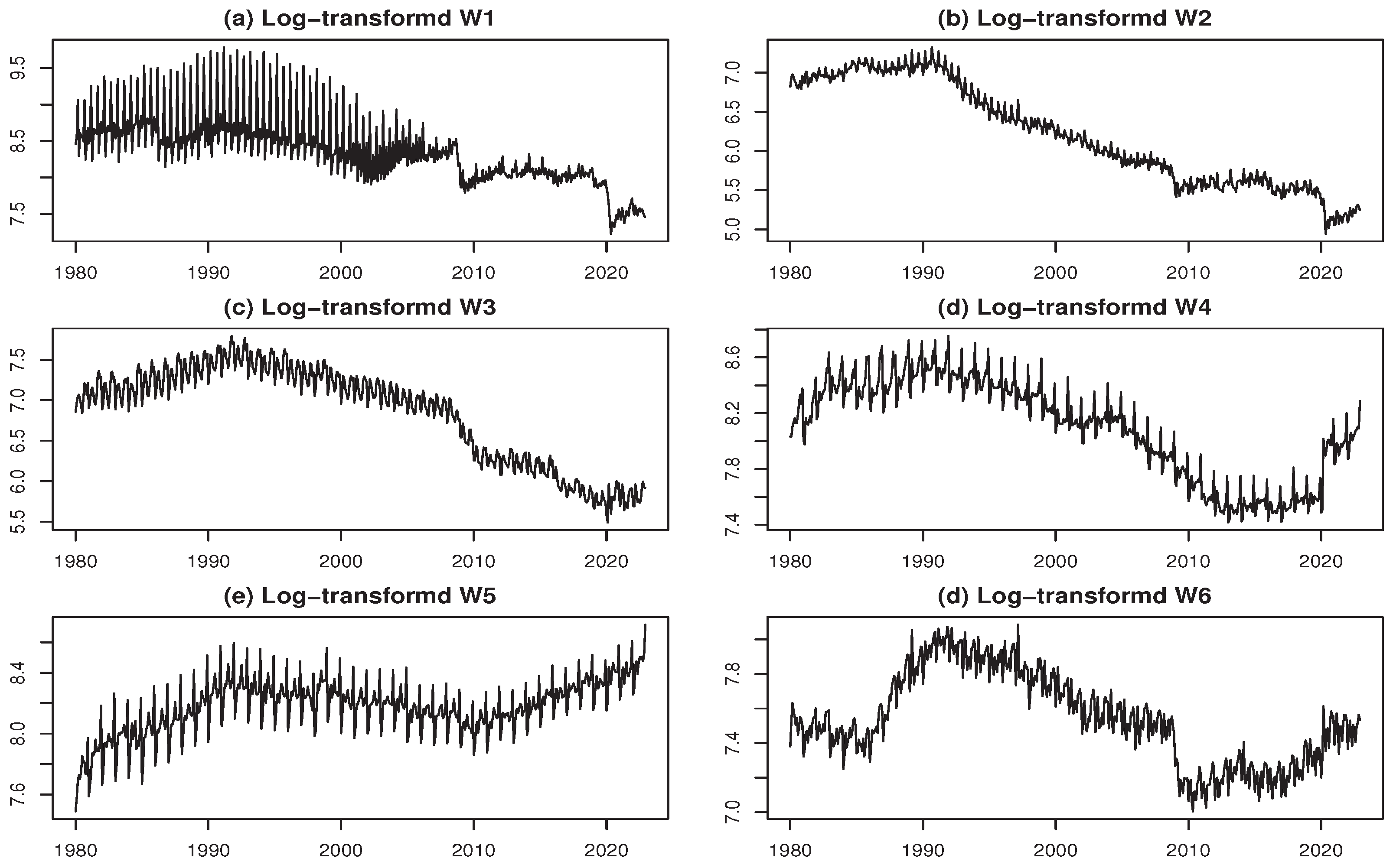
Figure 2.
log-WCS time series from W7 to W12 in Japan (January 1980 to December 2022)
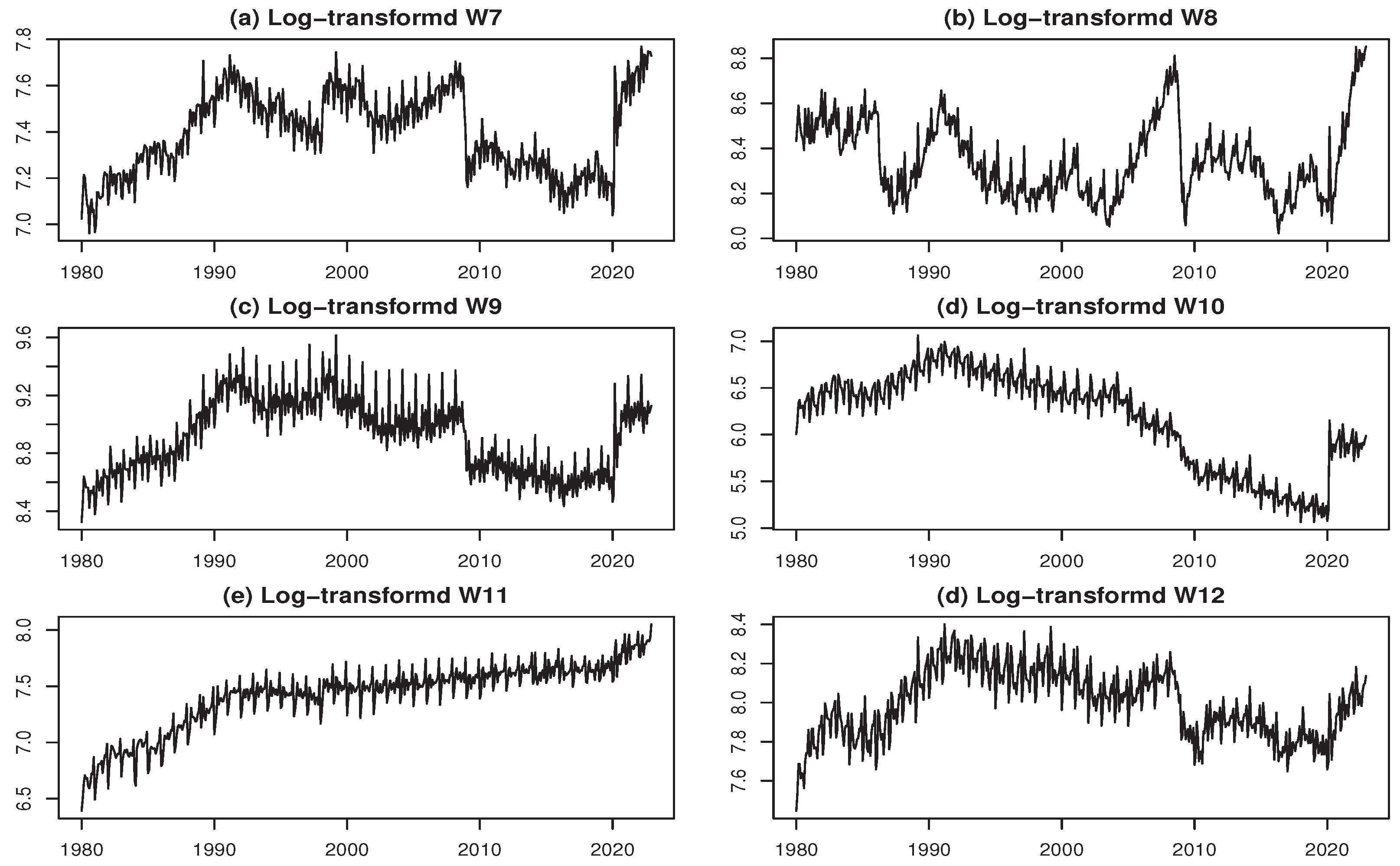
Figure 3.
Seasonally adjusted results for log-transformed time series of W1
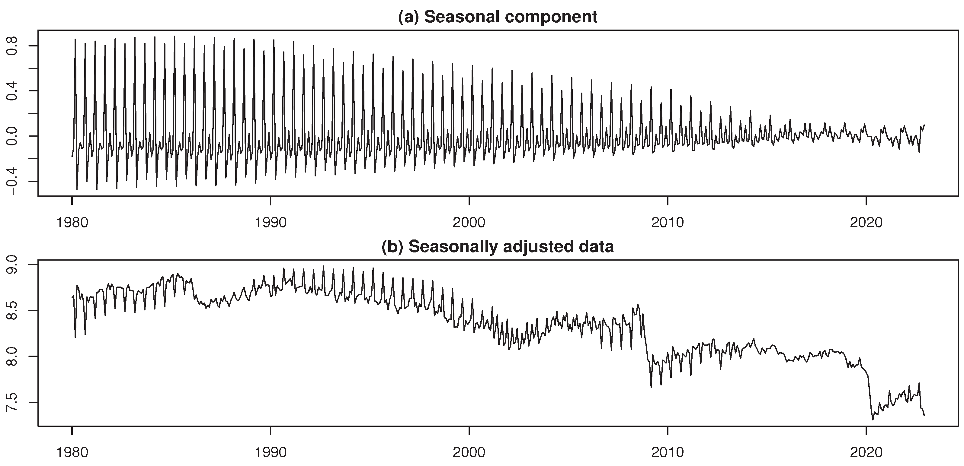
Figure 4.
Decomposed results for log-transformed time series of W1
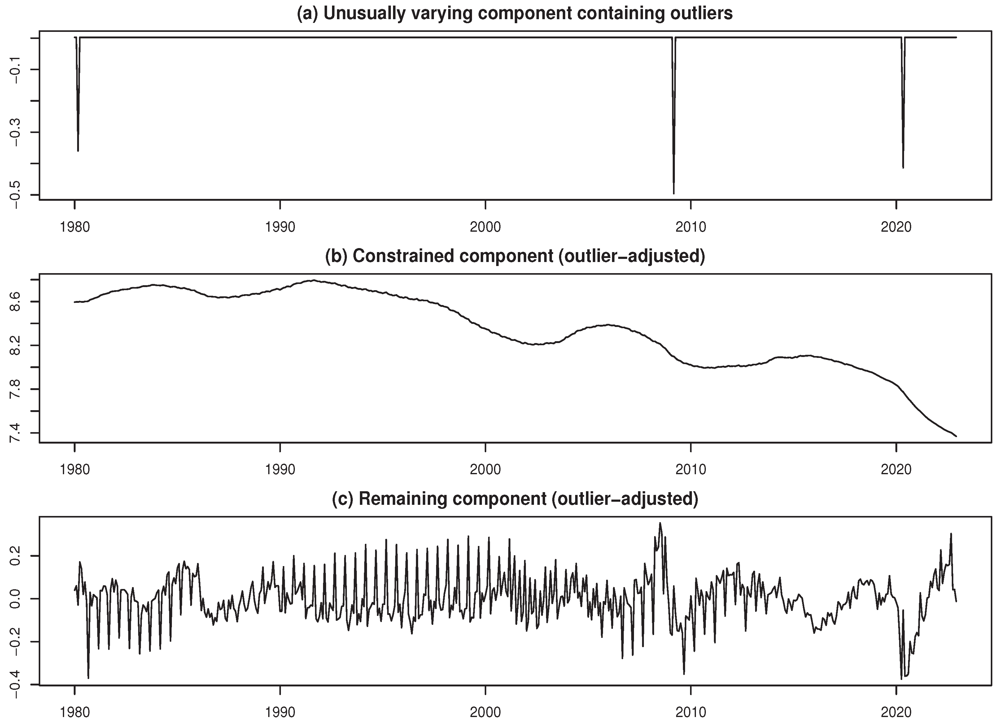
Figure 5.
Seasonally adjusted results for log-transformed time series of W2
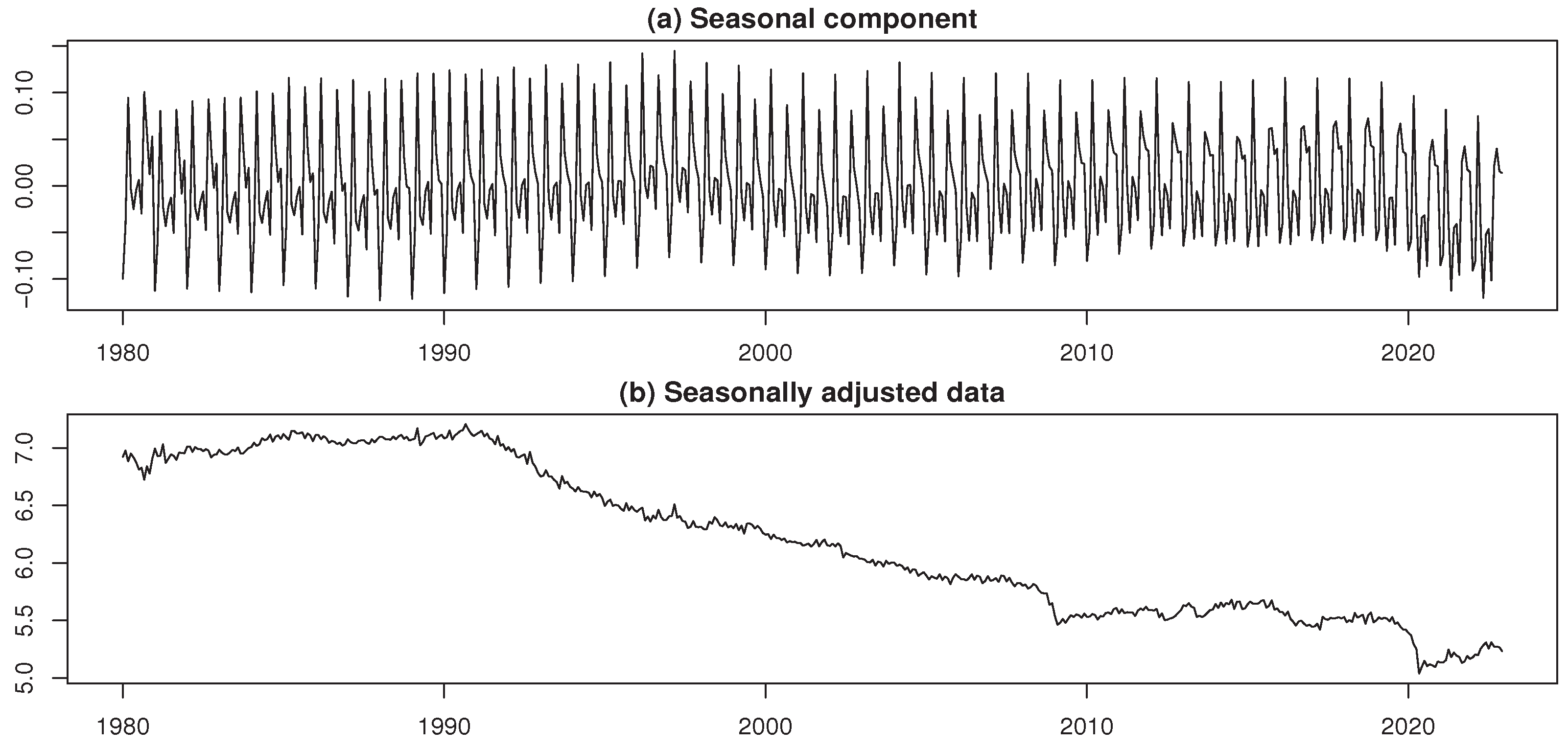
Figure 6.
Decomposed results for log-transformed time series of W2
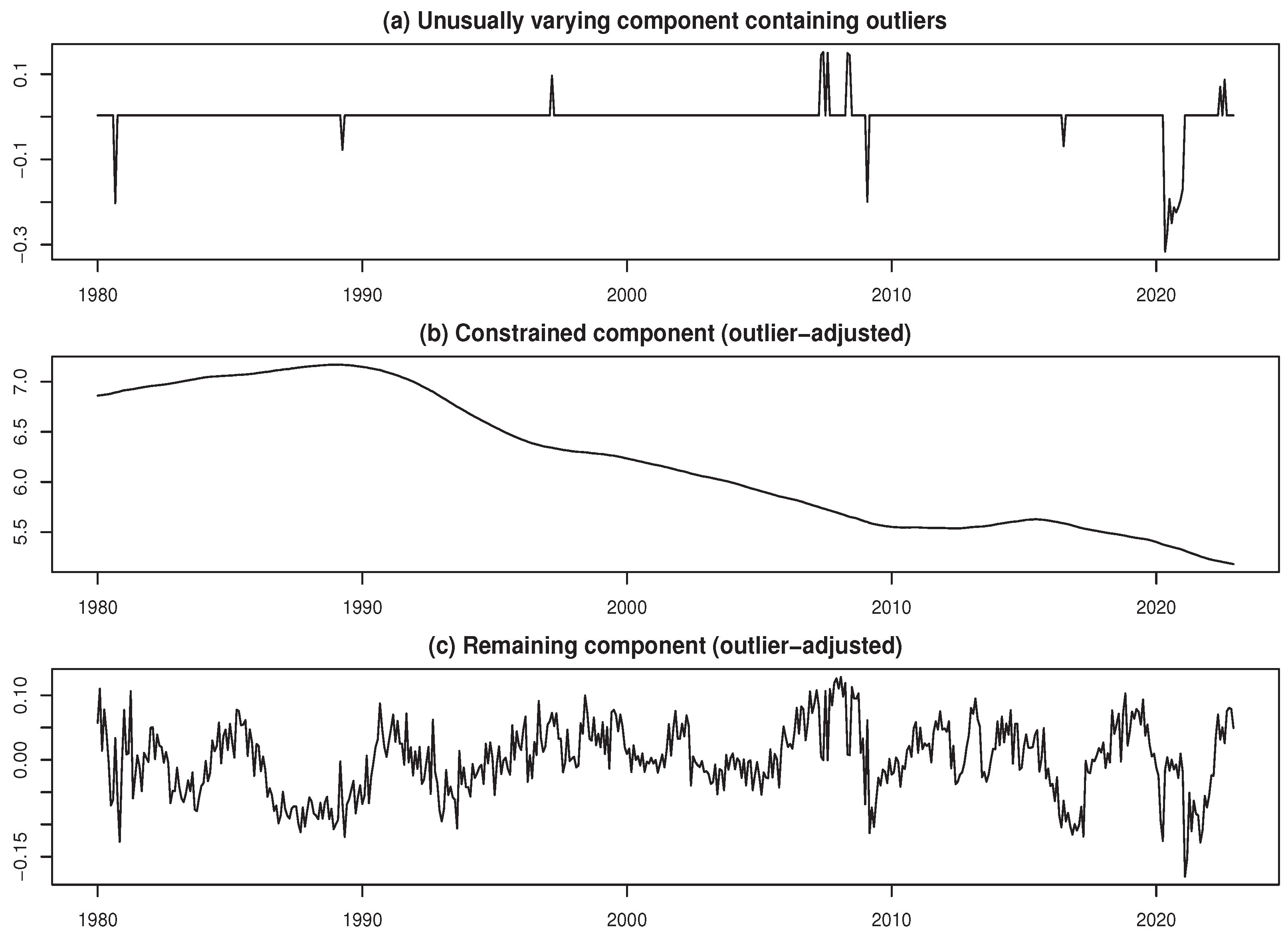
Figure 7.
Seasonally adjusted results for log-transformed time series of W3
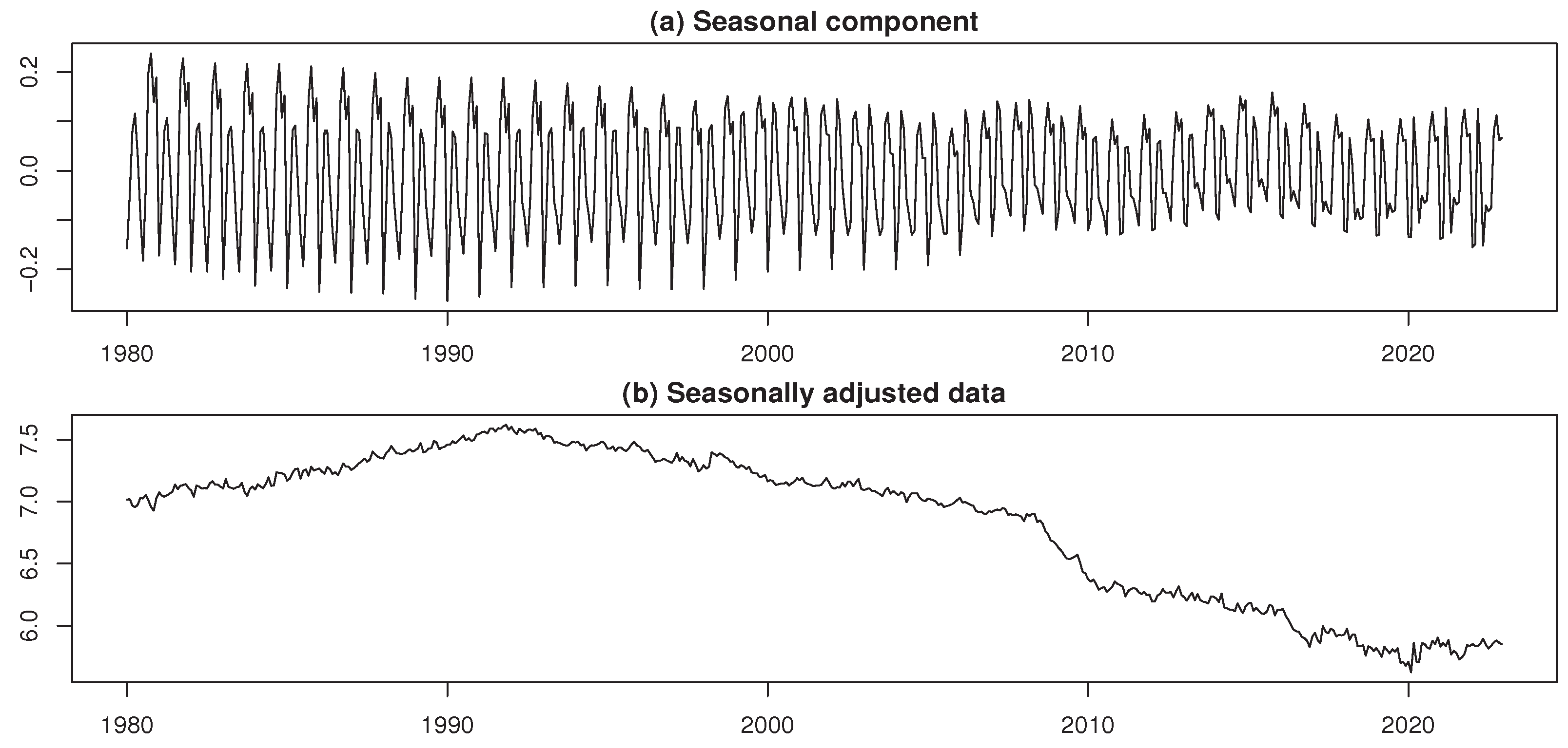
Figure 8.
Decomposed results for log-transformed time series of W3
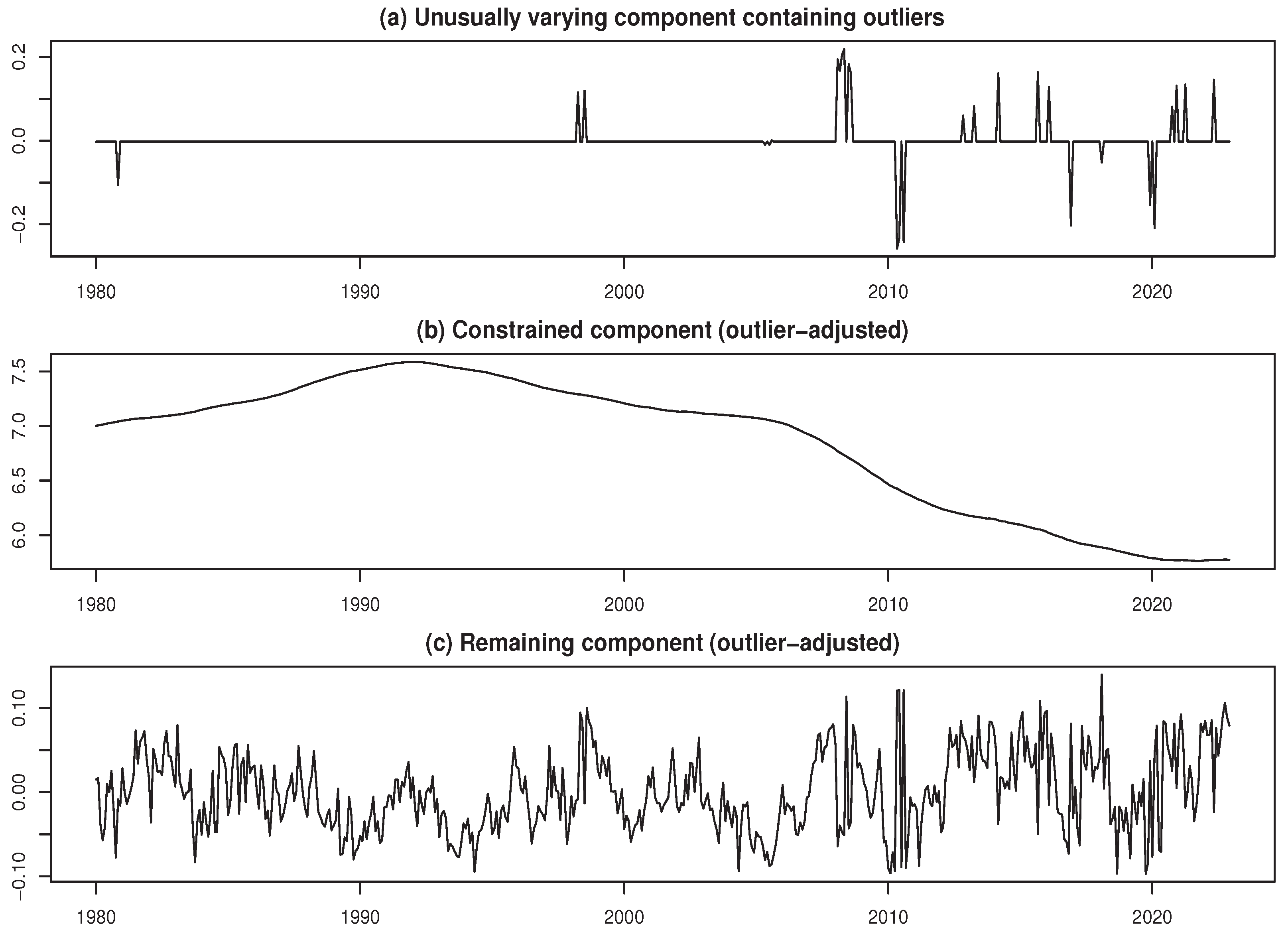
Figure 9.
Seasonally adjusted results for log-transformed time series of W4
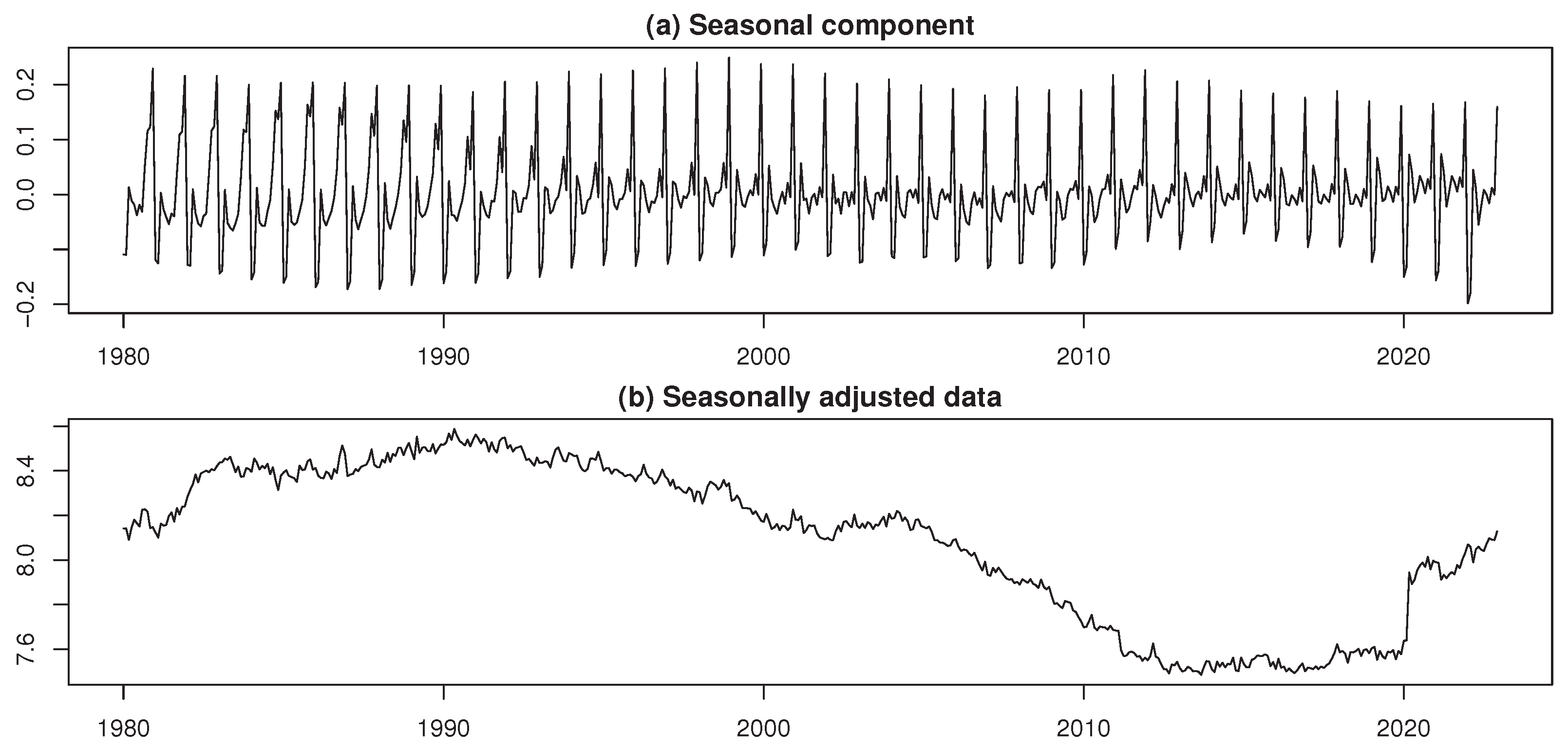
Figure 10.
Decomposed results for log-transformed time series of W4
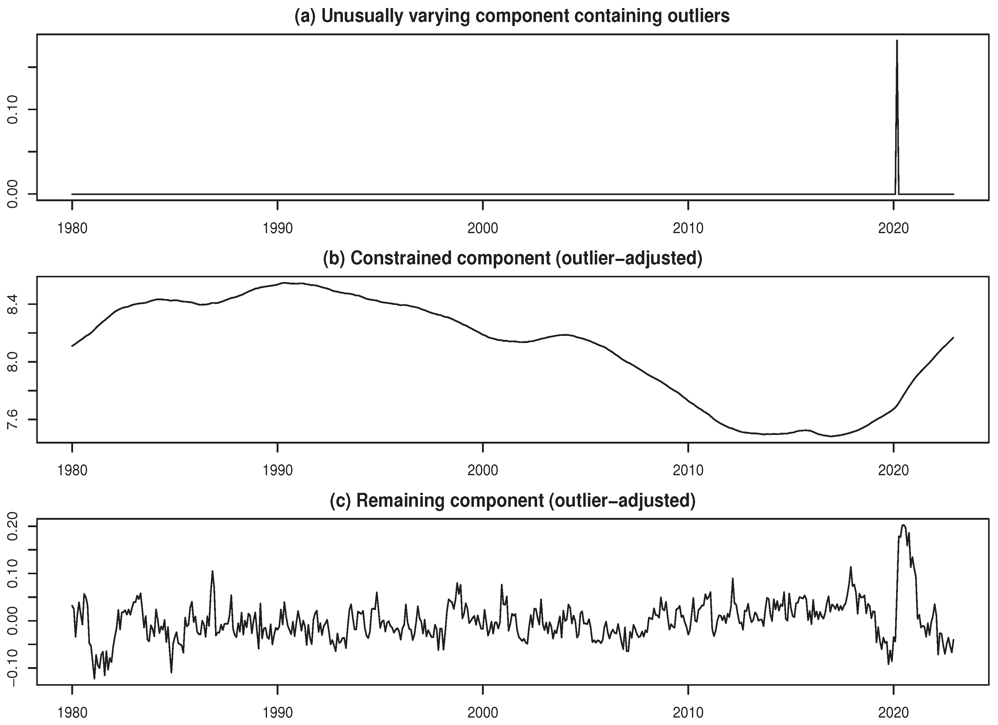
Figure 11.
Seasonally adjusted results for log-transformed time series of W5
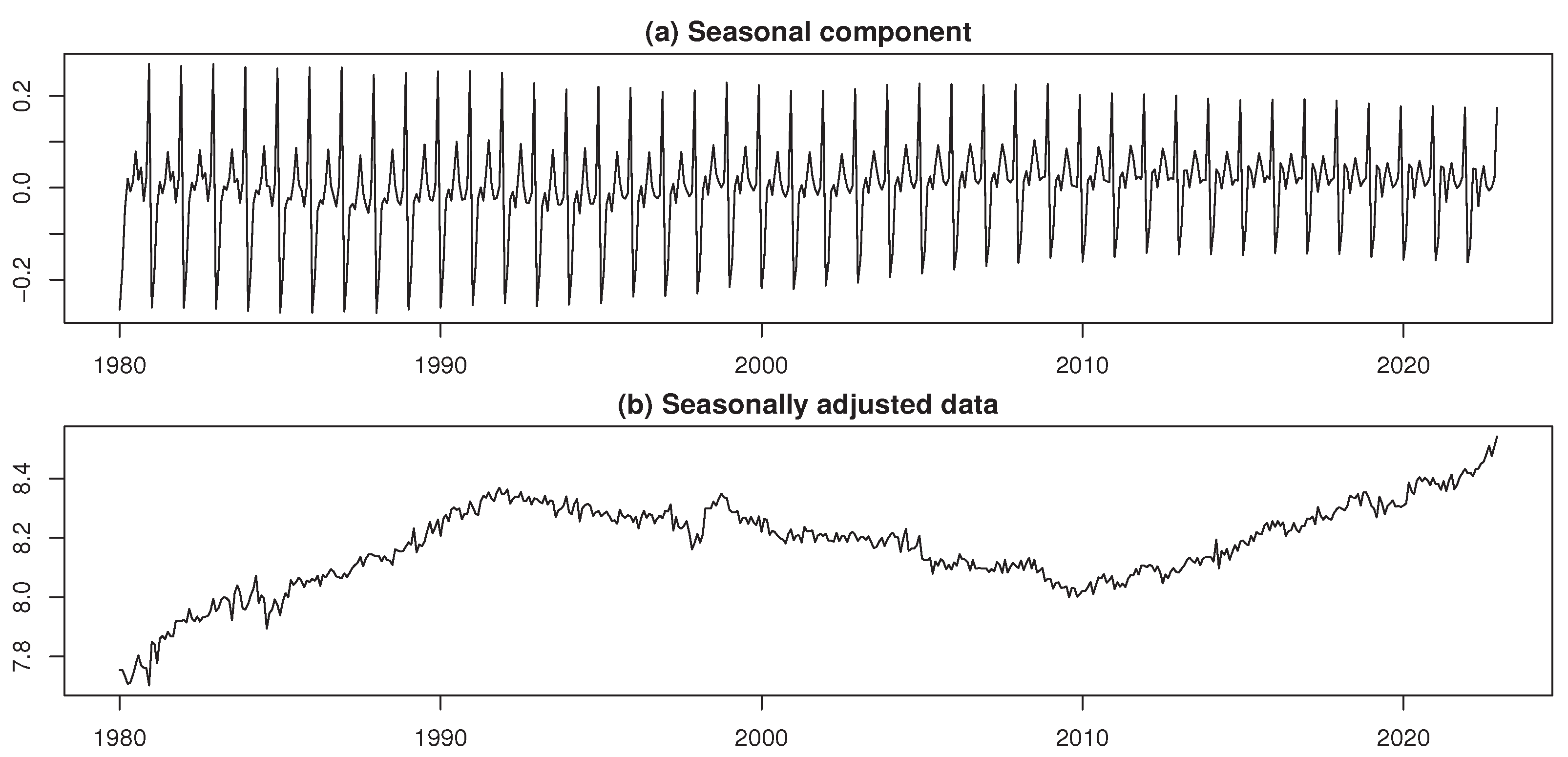
Figure 12.
Decomposed results for log-transformed time series of W5
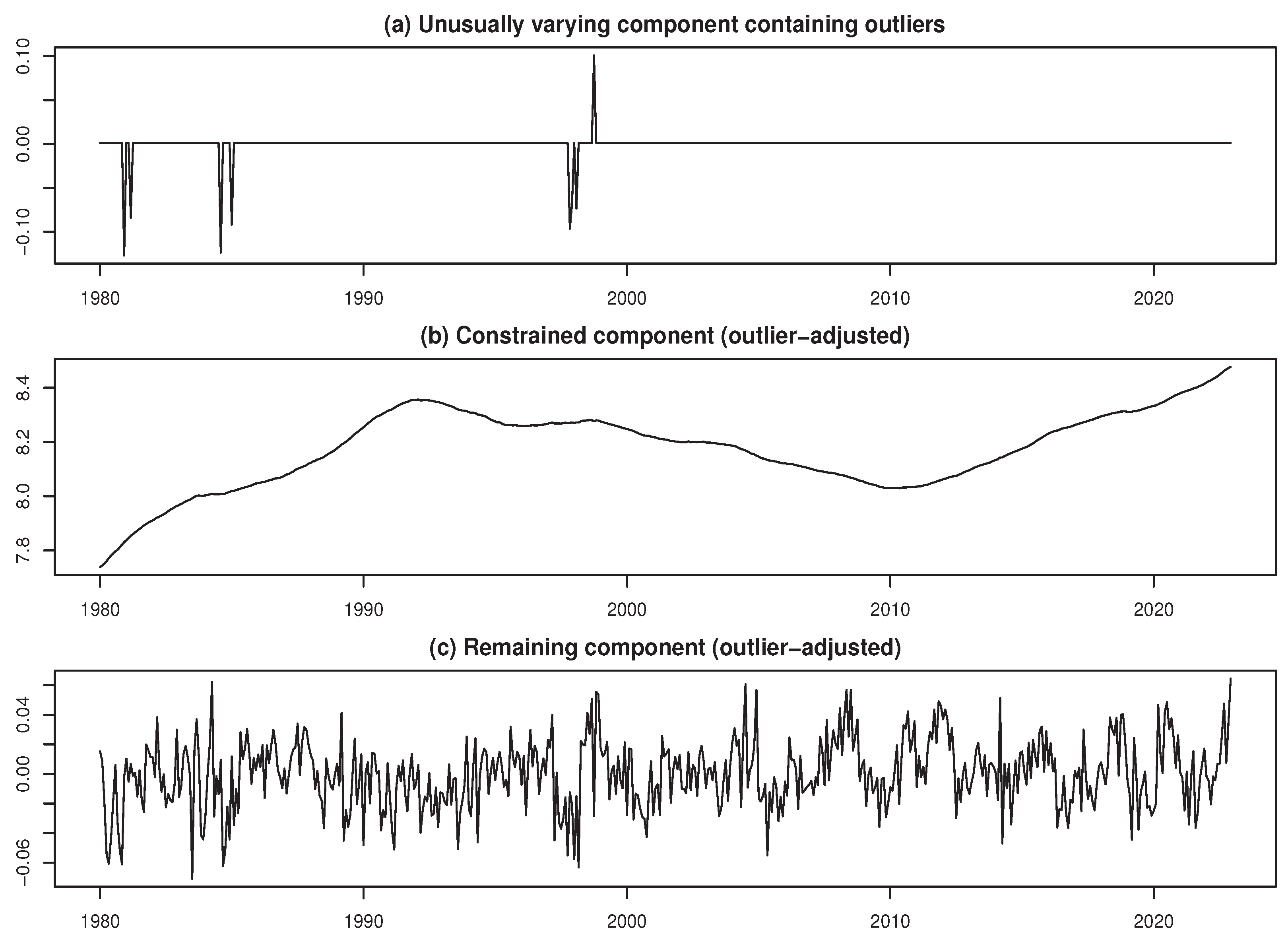
Figure 13.
Seasonally adjusted results for log-transformed time series of W6
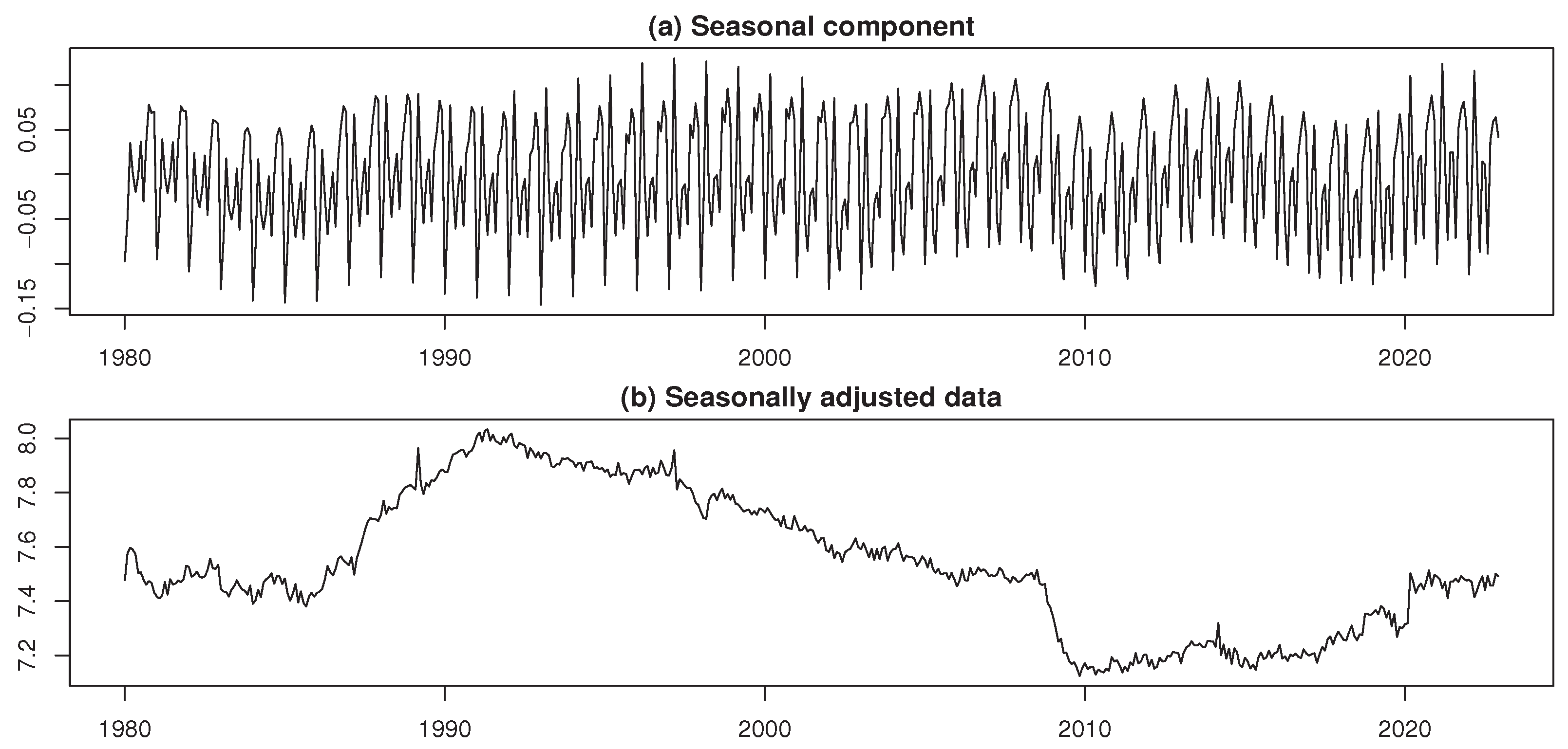
Figure 14.
Decomposed results for log-transformed time series of W6
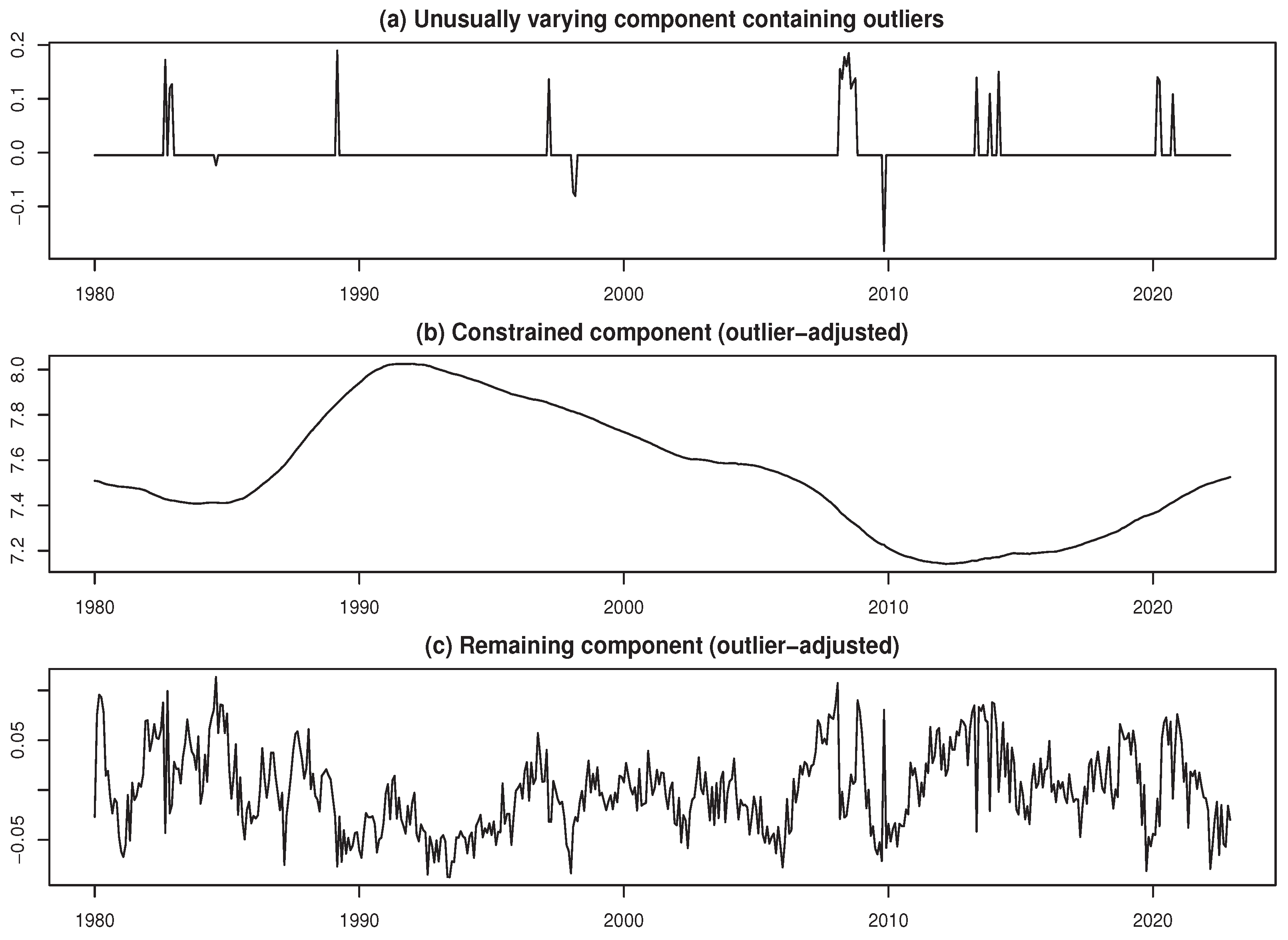
Figure 15.
Seasonally adjusted results for log-transformed time series of W7
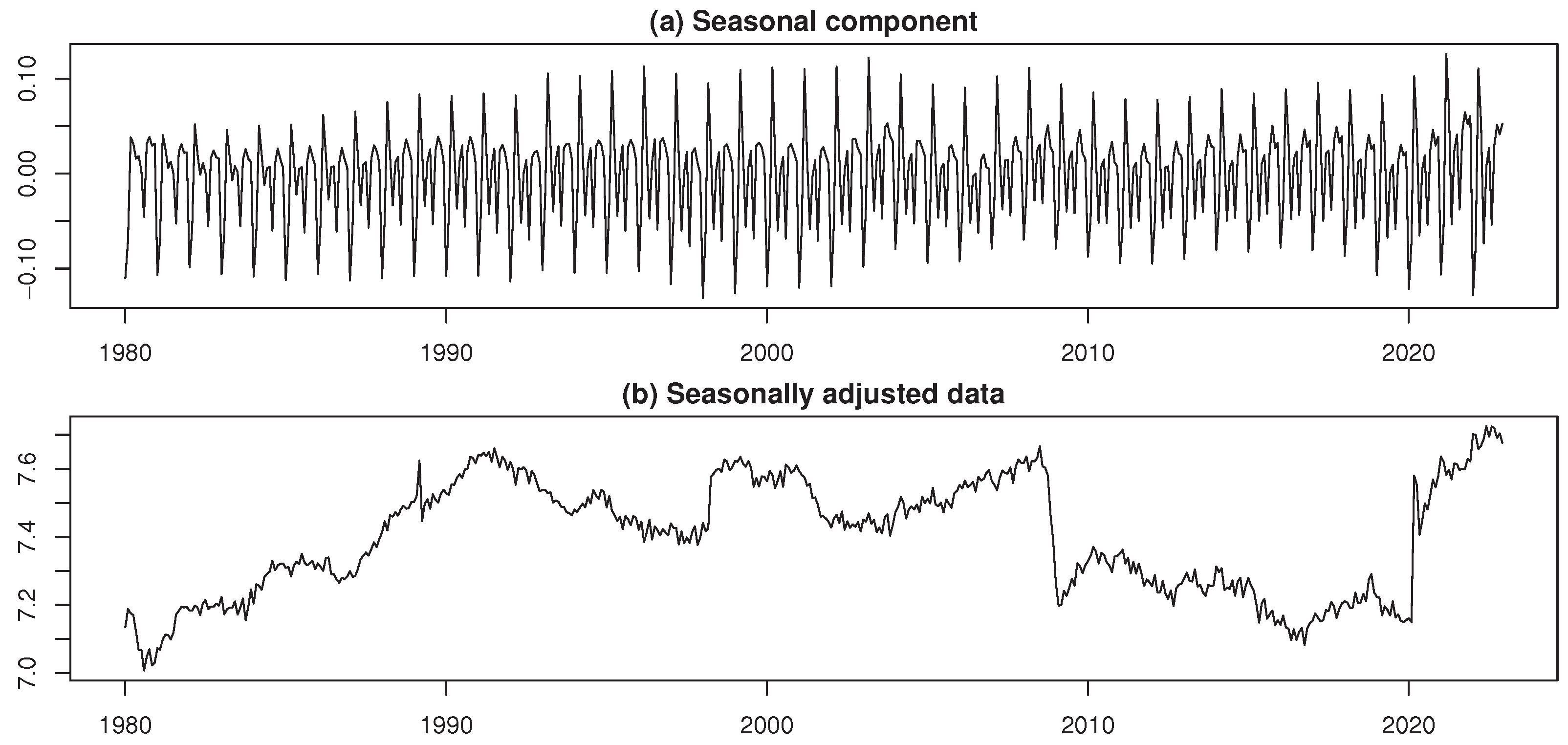
Figure 16.
Decomposed results for log-transformed time series of W7
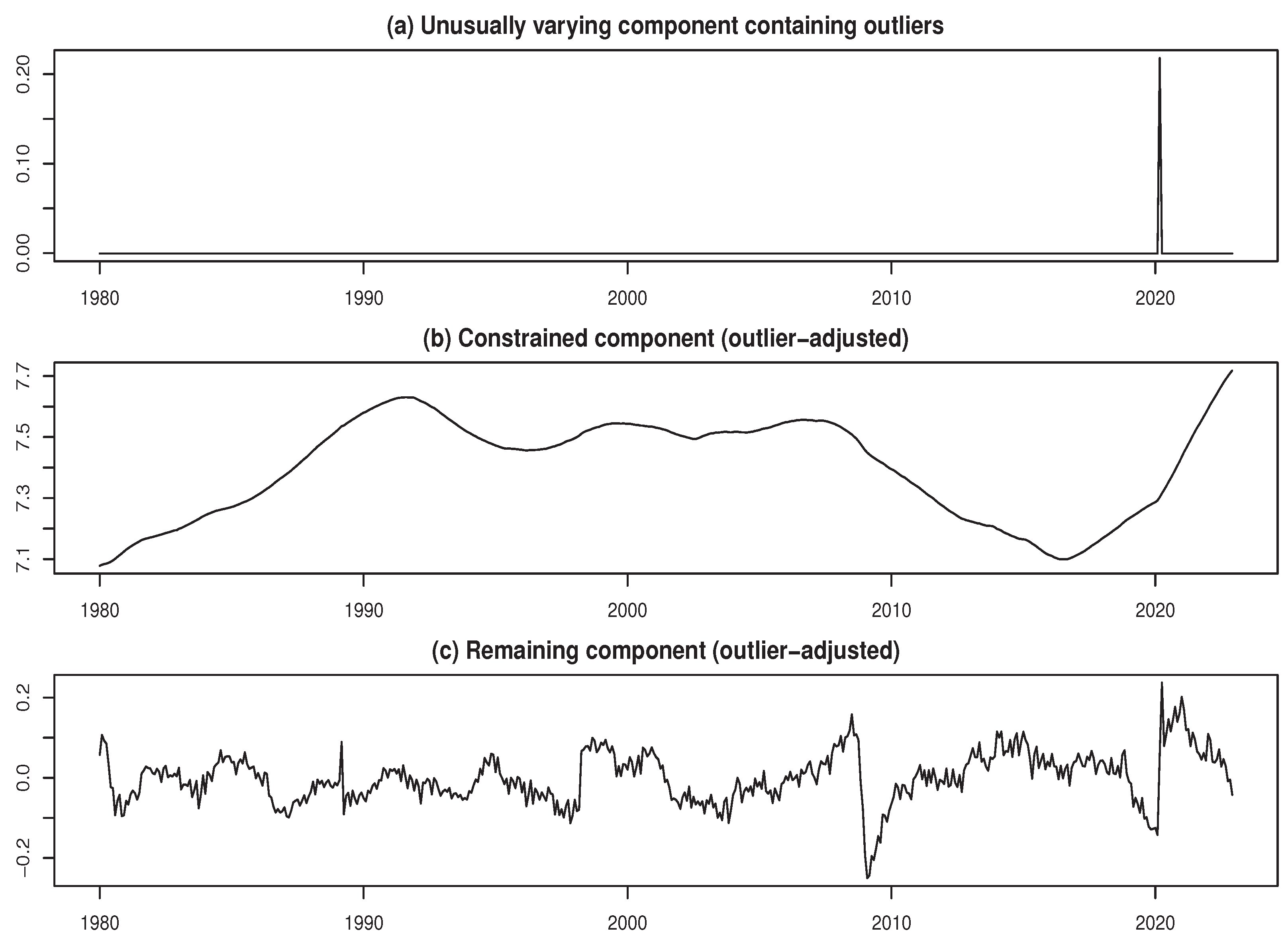
Figure 17.
Seasonally adjusted results for log-transformed time series of W8
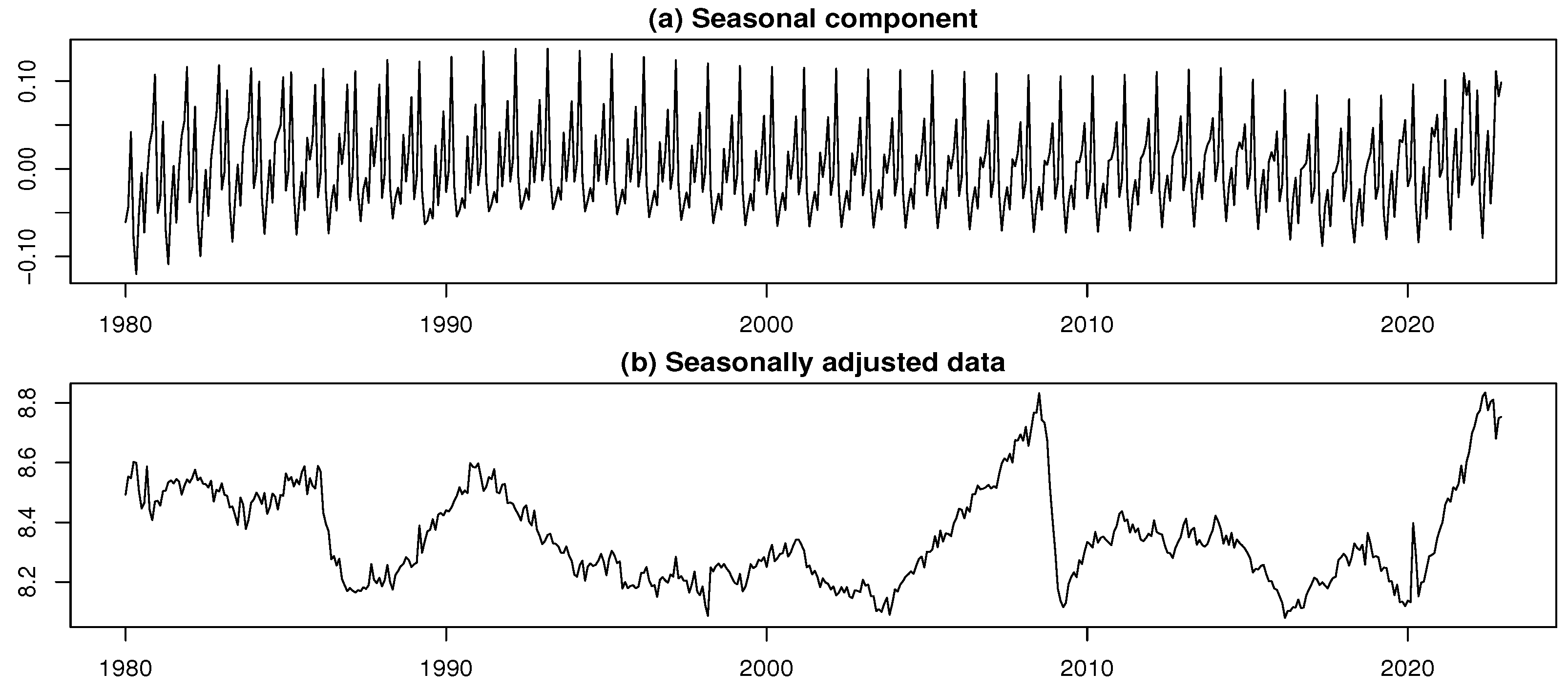
Figure 18.
Decomposed results for log-transformed time series of W8
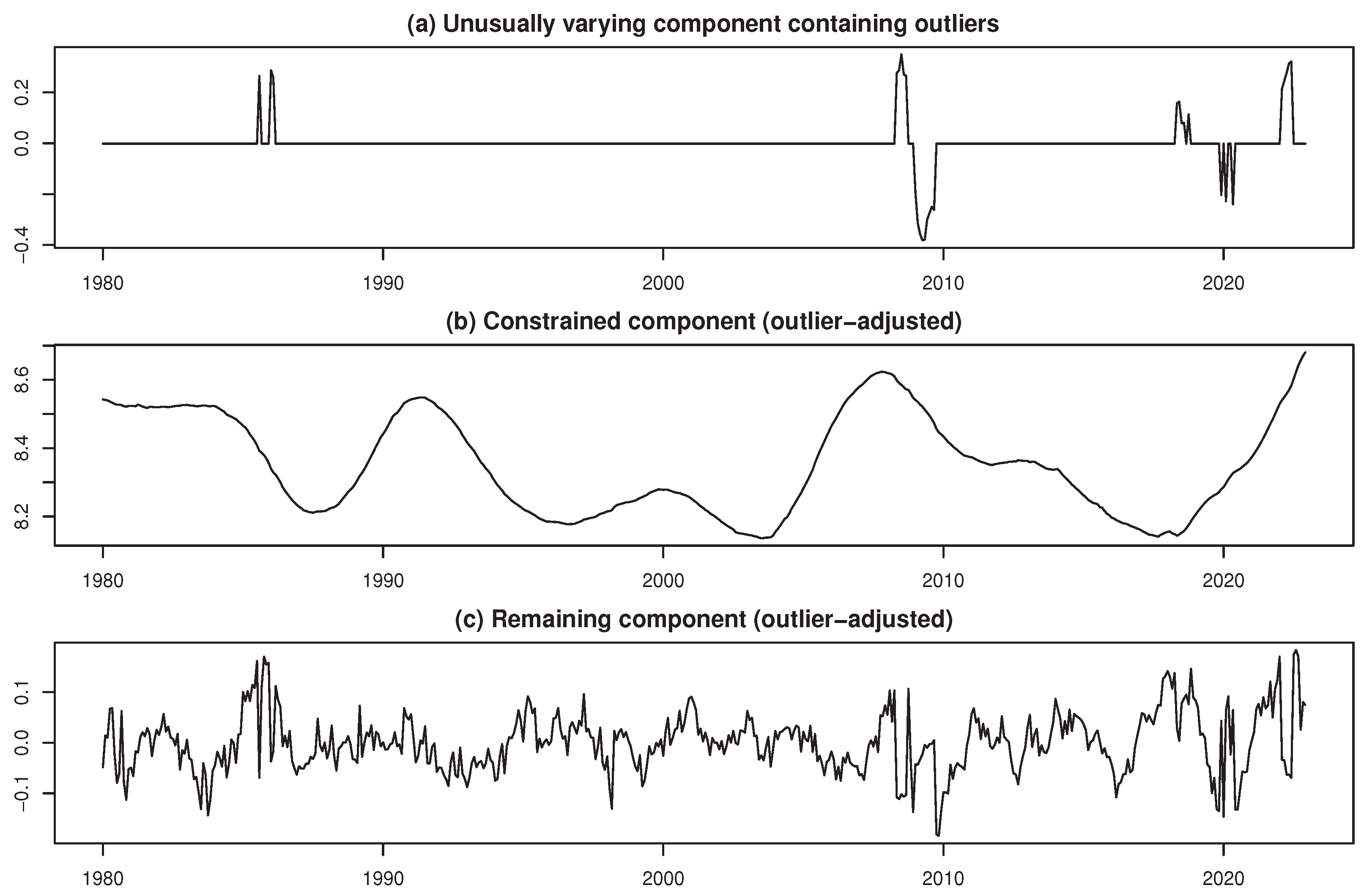
Figure 19.
Seasonally adjusted results for log-transformed time series of W9
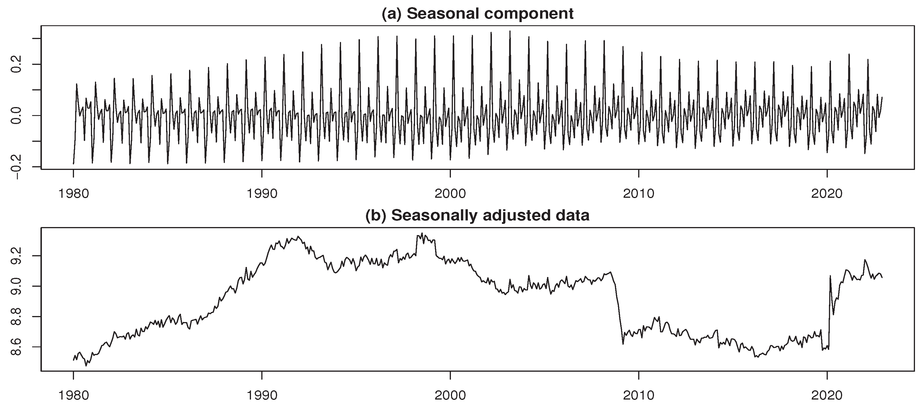
Figure 20.
Decomposed results for log-transformed time series of W9
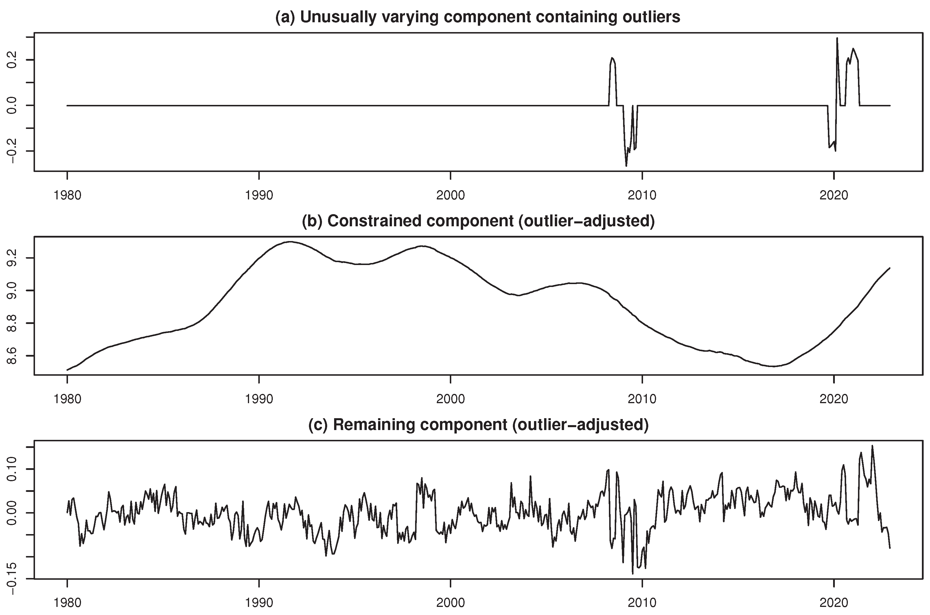
Figure 21.
Seasonally adjusted results for log-transformed time series of W10
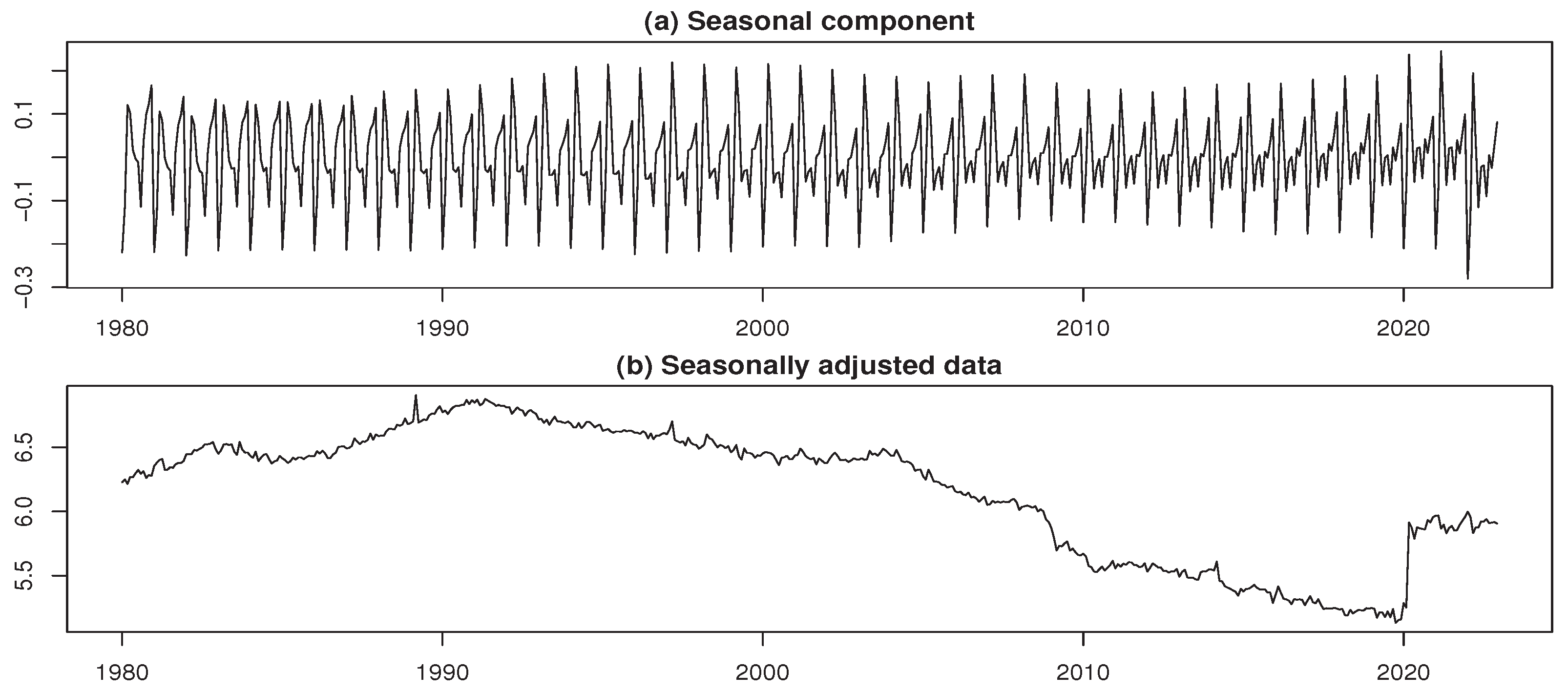
Figure 22.
Decomposed results for log-transformed time series of W10
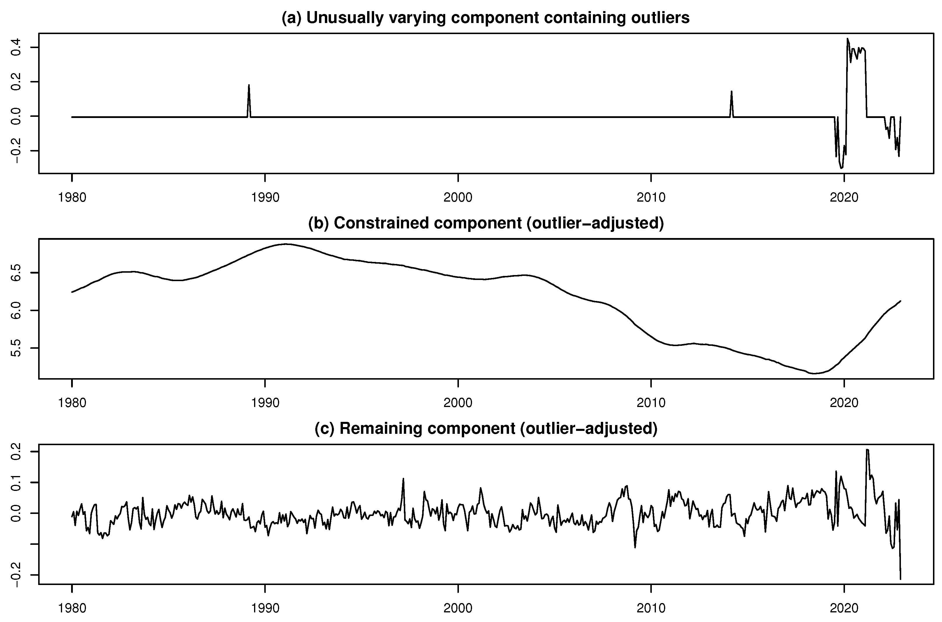
Figure 23.
Seasonally adjusted results for log-transformed time series of W11
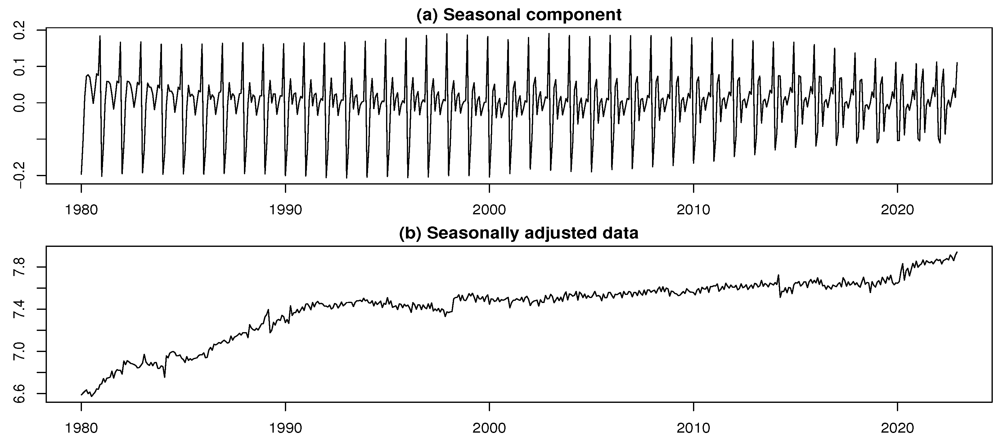
Figure 24.
Decomposed results for log-transformed time series of W11
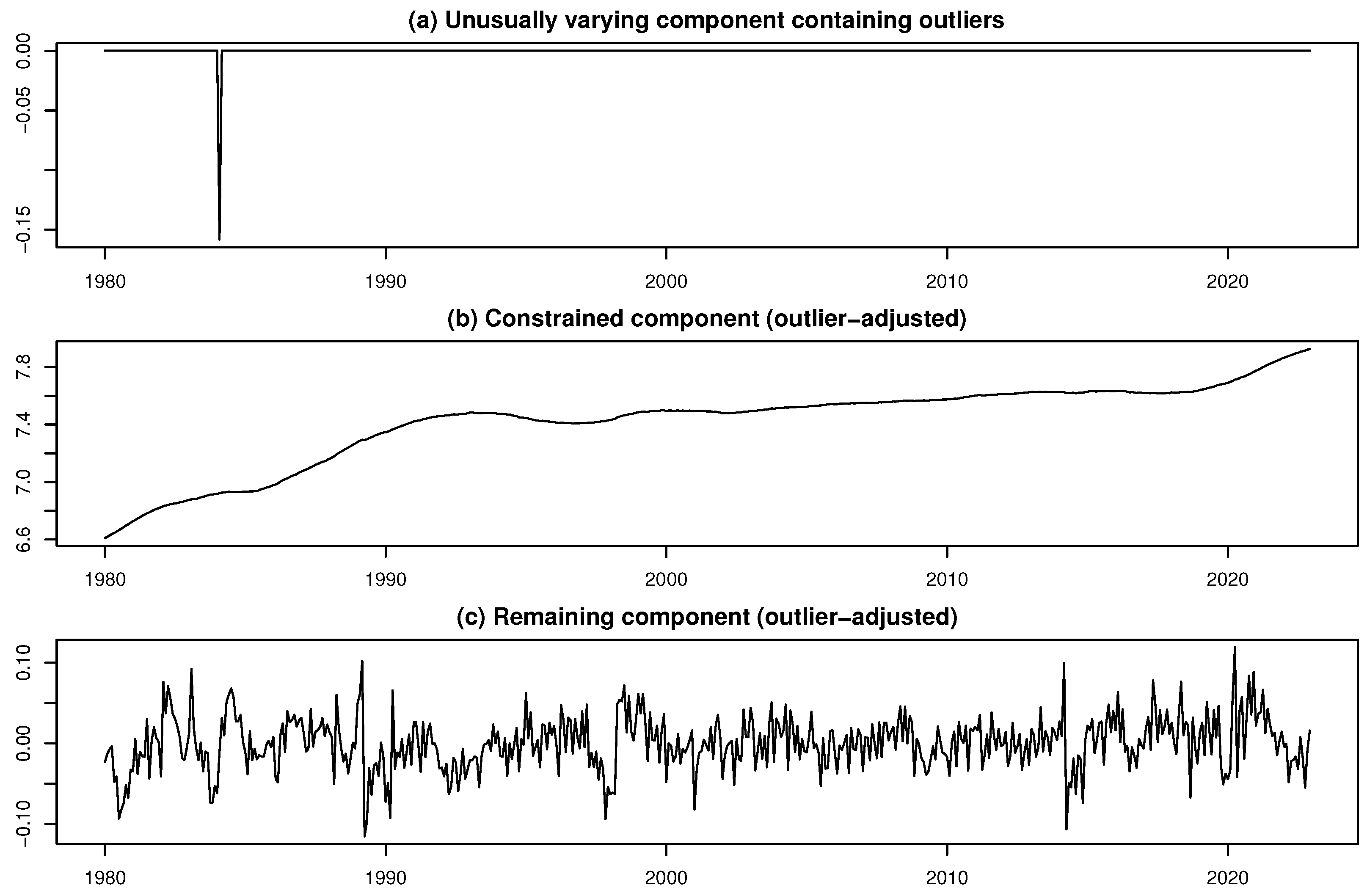
Figure 25.
Seasonally adjusted results for log-transformed time series of W12
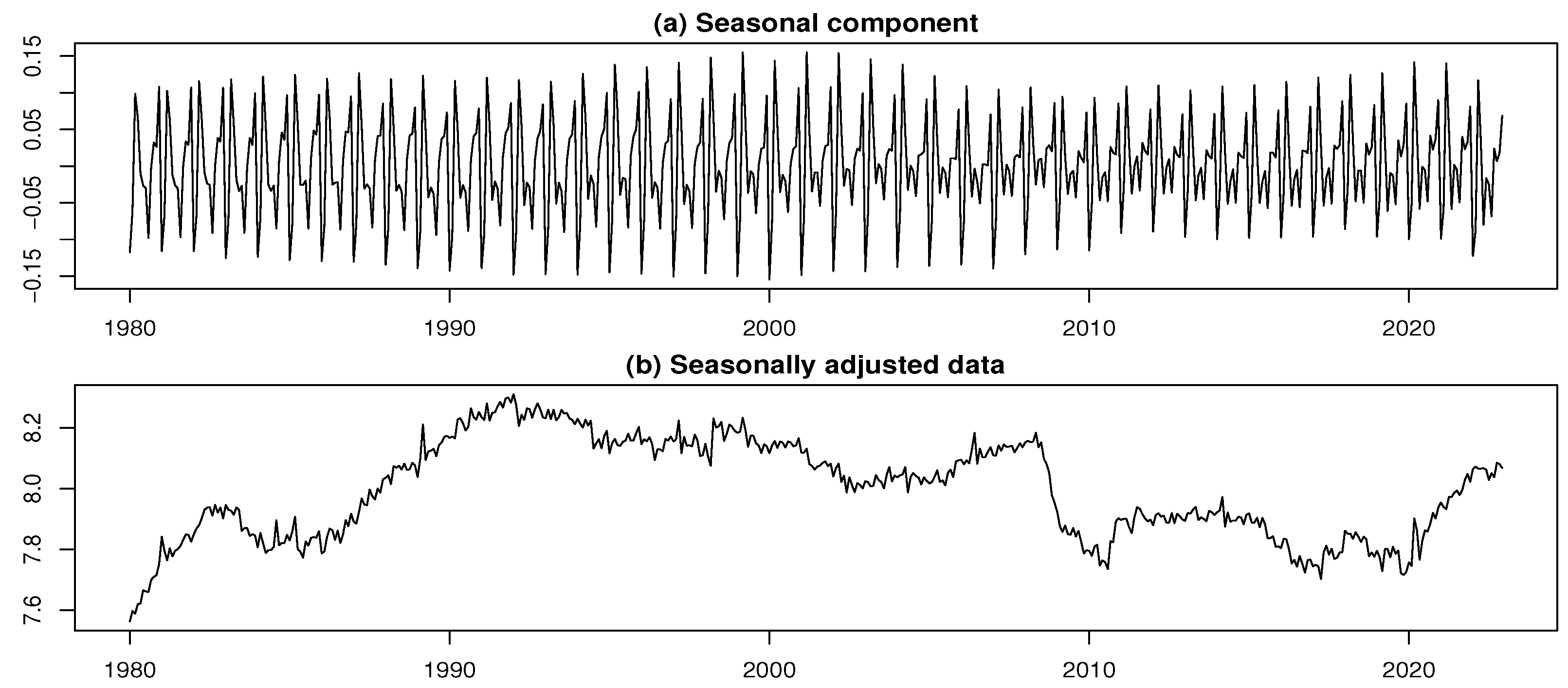
Figure 26.
Decomposed results for log-transformed time series of W12
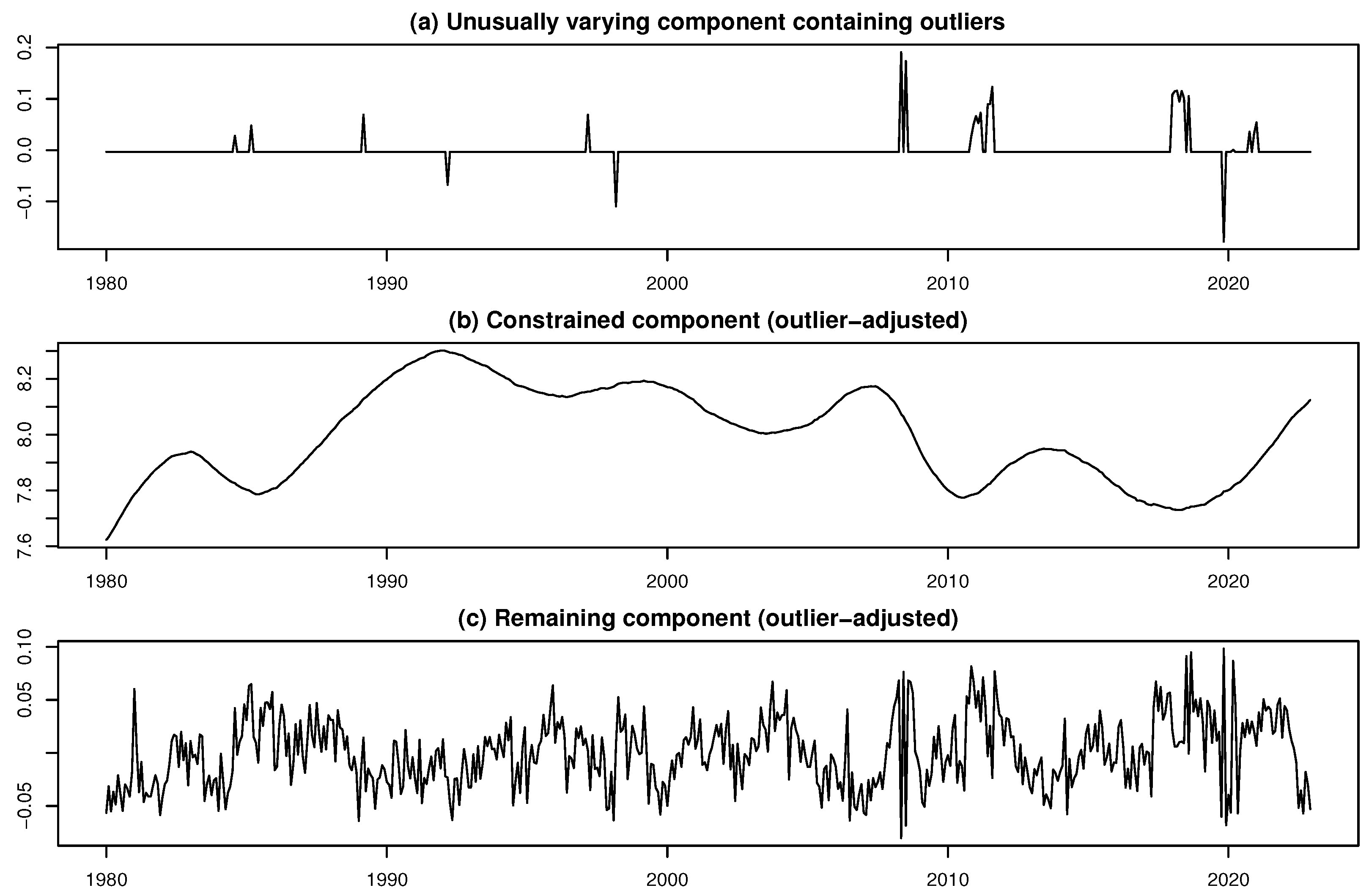
Figure 27.
log-CI time series in Japan (January 1985 to December 2022)
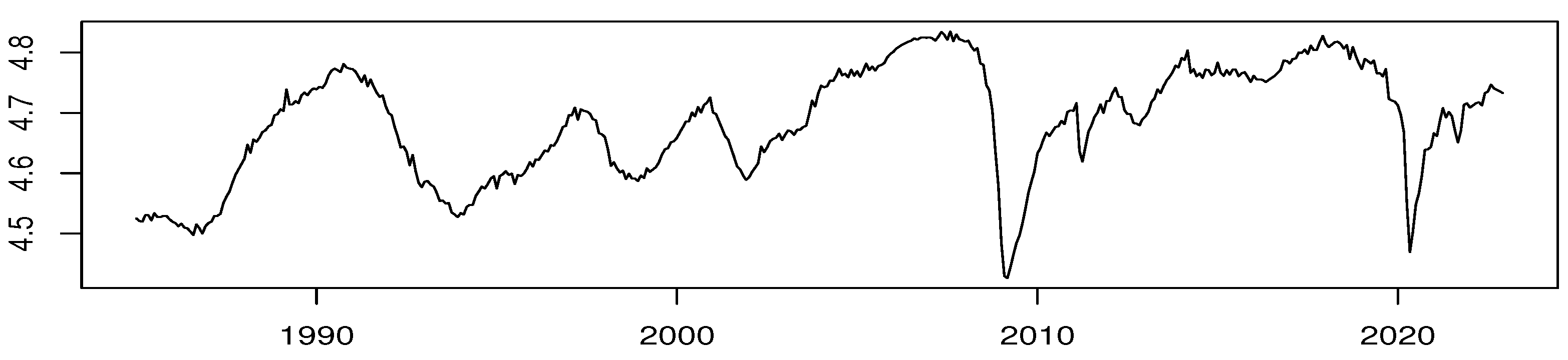
Figure 28.
Decomposed results for the time series of log-CI
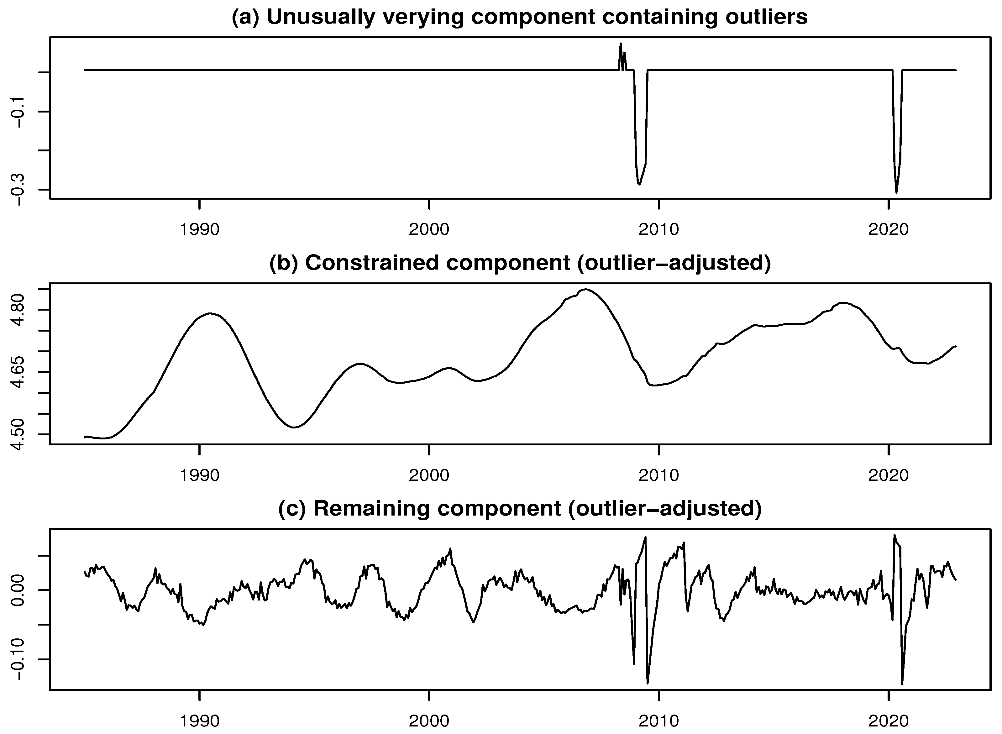
Figure 29.
Estimation results for time-varying coefficients in the models for W1–W4
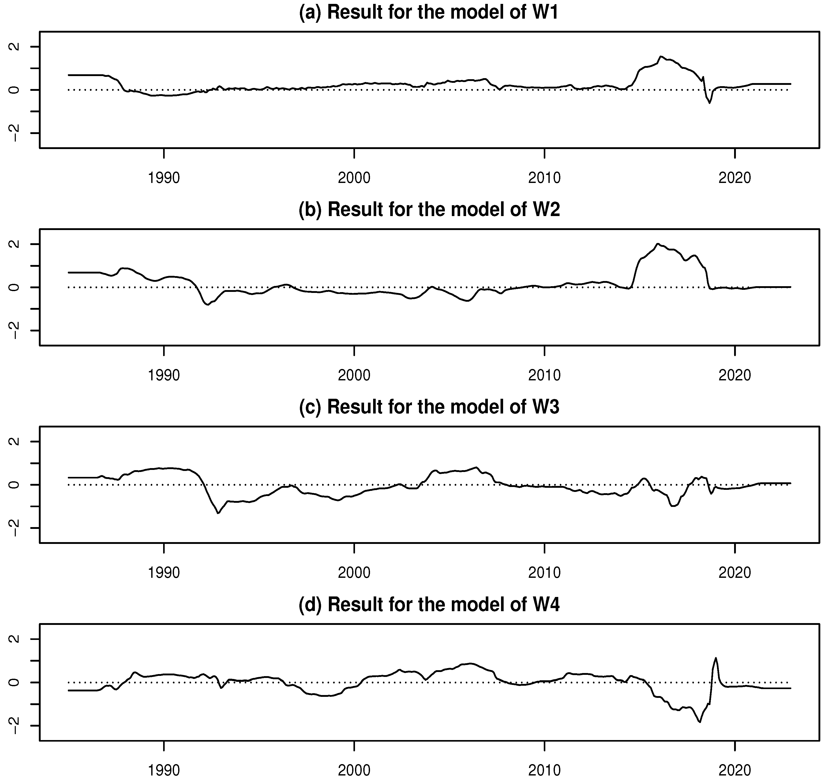
Figure 30.
Estimation results for time-varying coefficients in the model for W5–W8
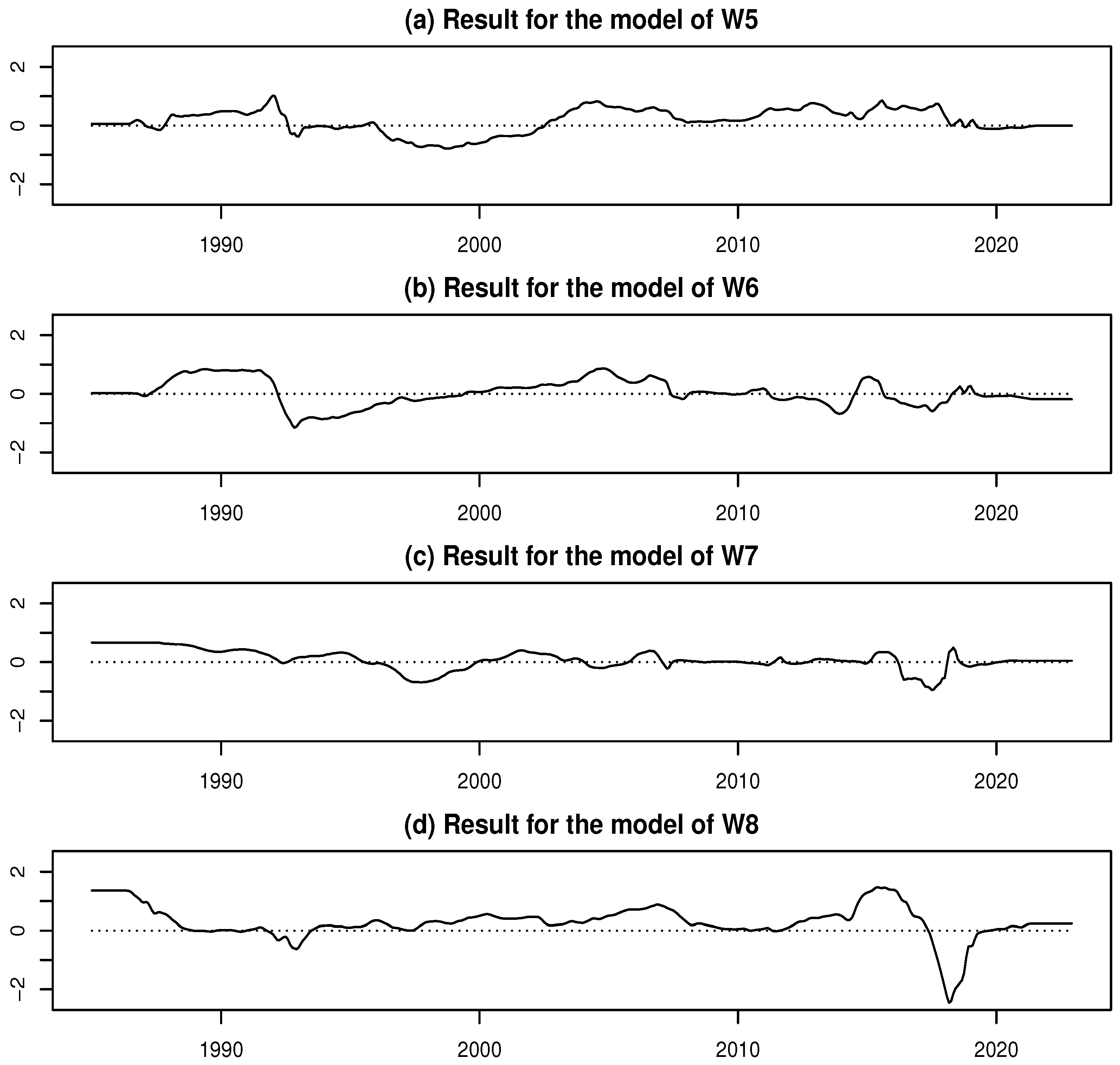
Figure 31.
Estimation results for time-varying coefficients in the models for W9–W12
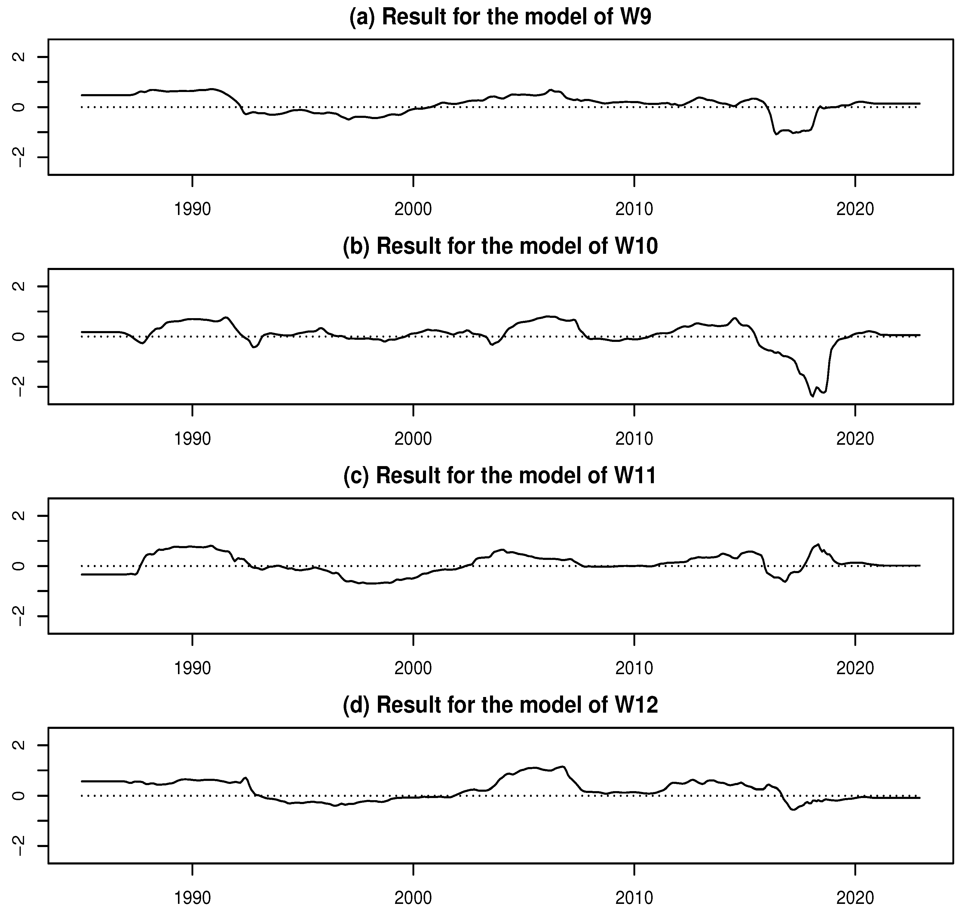

Table 1.
Business types of the wholesale commercial sales in Japan
| No. | Symbol | Name |
| No.1 | W1 | General Merchandise |
| No.2 | W2 | Textiles |
| No.3 | W3 | Apparel and Accessories |
| No.4 | W4 | Livestock and Aquatic Products |
| No.5 | W5 | Food and Beverages |
| No.6 | W6 | Building Materials |
| No.7 | W7 | Chemicals |
| No.8 | W8 | Minerals and Metals |
| No.9 | W9 | Machinery and Equipment |
| No.10 | W10 | Furniture and House Furnishings |
| No.11 | W11 | Medicines and Toiletries |
| No.12 | W12 | Others |
Disclaimer/Publisher’s Note: The statements, opinions and data contained in all publications are solely those of the individual author(s) and contributor(s) and not of MDPI and/or the editor(s). MDPI and/or the editor(s) disclaim responsibility for any injury to people or property resulting from any ideas, methods, instructions or products referred to in the content. |
© 2025 by the authors. Licensee MDPI, Basel, Switzerland. This article is an open access article distributed under the terms and conditions of the Creative Commons Attribution (CC BY) license (http://creativecommons.org/licenses/by/4.0/).
Copyright: This open access article is published under a Creative Commons CC BY 4.0 license, which permit the free download, distribution, and reuse, provided that the author and preprint are cited in any reuse.


