Submitted:
14 October 2025
Posted:
16 October 2025
You are already at the latest version
Abstract
Inverse pole figure mapping is a common orientation visualization method used in electron backscatter diffraction (EBSD) software to display crystal orientations. Although this technique has been routinely used in commercial EBSD software, the coloring algorithm employed to map the orientation and construct the color key (standard stereographic triangle) has not been reported in the literature. This paper presents a simple algorithm to color the standard stereographic triangles of the 11 Laue groups by mapping the Maxwell color triangle to the curved standard stereographic triangles using nonlinear shape functions commonly employed in finite element methods. Detailed procedures are given to illustrate how the mapping is performed and how it is used to construct inverse pole figure maps from Euler angles. Color coding of the 7 different standard stereographic triangles is demonstrated using a computer program written in C++. It is shown that the simple color-coding algorithm presented in this paper can be conveniently utilized to display orientation data in inverse pole figure maps which is a critical part of designing customized EBSD software. It also provides a method to adjust the color center within the curved triangles to more uniformly distribute the color, which is not available in commercial EBSD software. The algorithm can also be used to design orientation representation software for other applications, e.g., crystal plasticity simulations, where representation of orientation data is also a routine task.
Keywords:
inverse pole figure mapping
; electron backscatter diffraction
; standard stereographic triangle
; color coding
; finite element methods
; shape functions
Introduction
Since the first automated electron backscatter diffraction (EBSD) systems were commercialized in the 1990-2000’s (Wright, et al., 1991; Dingley & Randle, 1992; Adams, et al., 1993; Randle & Engler, 2000; AMETEK Inc., 2019; Oxford Instruments, 2009), they have become an indispensable characterization tool in material science to obtain both the microstructural and crystallographic information of materials. The use of this technology has helped scientists and engineers understand many metallurgical phenomena that could not be comprehended using other technologies. When displaying EBSD data, inverse pole figure (IPF) mapping is most used to illustrate the crystal orientations with respect to the specimen axes. Each IPF map shows the parallelism of the lattice planes (normals) or directions of the crystals in the specimen to a specific specimen axis. Normally, one IPF map cannot show the complete crystal orientation since it only illustrates the correlation between one specimen axis and the crystal planes or directions. Nevertheless, one IPF map is normally enough to illustrate how differently the crystal lattice planes (or directions) in a specimen are aligned to a specific specimen axis. When displaying IPF maps, a color key, also known as standard stereographic triangle (SST), must always be presented together with the map to indicate the specimen axis to which the normals to the crystal planes or the crystal directions are parallel.
While commercial EBSD software provides such a convenient tool to display EBSD data, the algorithm used to color the SST and to correlate each point in the color key (SST) to a specific pixel in the IPF map has not been reported in the literature. Intuitively, the color of each point in the SST and that of the corresponding pixel in the IPF map should be directly correlated to the orientation itself, i.e., ideally the color should have some meaning related to the crystal orientation. Nolze and Hielscher used the azimuthal and polar angles of an orientation on the projection sphere to determine the hue and lightness (the saturation is set to 1) of the HSL (hue, saturation, and lightness) coloring scheme, which leads to meaningful coloring of the orientations. Although with the benefits of avoiding color jumps and producing a homogeneous color variation, both the hue (azimuthal angle) and lightness (polar angle) must be modified using some functions to render evenly distributed colors. As a result, it is not straightforward to reveal the information of the orientation (defined by the angles) from the color after such a transformation. It should be noted that, for IPF mapping in EBSD, the color is essentially just a “tool” to facilitate the visualization of many orientations on the map; it is not necessary to have a meaning of the orientation itself. Thus, if the color can be unequivocally distinguished in the SST and displayed in the IPF map, it does not matter what coloring scheme is used. As a result, there might be many ways to color the SST and thus mapping the orientations.
This paper presents a few color-coding techniques, e.g., Miller indices, barycentric coordinates, and finite element shape functions, to color the SSTs. These coloring schemes are purely based on the shapes of the SSTs. It is demonstrated that color-coding using nonlinear shape functions is simple and easy to implement and can be used for all crystal symmetries. For the coloring using shape functions, the Maxwell color triangle (MCT), a standard equilateral triangle with the three vertices colored red, green, and blue (the RGB color model), is used as the reference triangle (like in finite element methods) and mapped to the curved SSTs. The reference coordinates (also representing the color components of red, green, and blue) of each point in the reference triangle are used to represent the color of the corresponding point in the curved SSTs. The geometric mapping between the reference triangle and the real curved SSTs using shape functions is similar to the isometric triangulation technique commonly employed in finite element meshing. The formulation and application of these methods to the SSTs of the 11 Laue groups are presented in detail. A C++ program using the OpenGL graphics library is developed to display the colored SSTs as well as the IPF maps obtained from EBSD measurements. IPF maps of the same EBSD data set using these methods are compared to the map displayed using commercial EBSD software and only very small difference is noticed. The color-coding method presented in this paper may be used to develop customized EBSD software or display orientation data obtained from crystal plasticity simulations.
Geometry of SSTs for All Crystal Symmetries
To develop a general color-coding technology for EBSD IPF mapping, SSTs for all crystal symmetries (differentiated in the 11 Laue groups) should be determined first. It is known that there are 32 point groups, but the symmetries of these point groups can be distinguished by the 11 Laue groups in EBSD. Due to crystal symmetry, a lattice plane or direction usually has multiple equivalent poles in stereographic projection (Whittaker, 1981; He, 2023). For inverse pole figure mapping, only a representative portion of the entire projection is needed (the so-called standard stereographic triangle), i.e., an SST is enough to represent the relation between the lattice planes (or directions) of the crystals and the specimen axis. Of the 11 Laue groups, only 9 of them form a real "triangle" (the other two are either a circle or a semi-circle) (Oxford Instruments, 2009; He, 2023). Of the 9 Laue groups that have well-defined SSTs, only 7 shapes are distinguished. Five of these 7 shapes are a sector of a unit circle centered at (0,0) (bounded between two radii and an arc), see Figure 1a; the rest 2 are portions of a 45°-sector of a circle with a radius of centered at the end of a diameter, for example, (-1, 0), see Figure 1b.
The curved side of each of the 5 sectors (SSTs) is a part of a unit circle (r = 1) centered at (0, 0), and the two straight sides are the radii (Figure 1a). In the two SSTs for cubic low and cubic high symmetries (portions of a 45°-sector), the curved side is a part of a circle with a radius of centered at (-1, 0) and the two straight sides are either a radius or a portion of a radius centered at (0, 0). The vertices of these SSTs can be readily determined from the sector angles in the unit circle (Figure 1c and Figure 1d). The vertices of the SST for cubic high symmetry are at the 001, 011 and 111 poles, while those for cubic low symmetry are at 001, 010 and 111.
Color Coding of SSTs
In an SST, each point represents a lattice plane (the normal to the plane) or lattice direction stereographically projected onto the equator plane of a unit sphere centered on the origin of the crystal. These lattice planes or directions are denoted by their Miller indices ({hkl} or <uvw>) or Bravais indices ({hkil} or <uvtw>). With the increase of the maximum integers in the Miller/Bravais indices, the SST is gradually filled up with the projected poles. For example, for cubic crystals (point group m3m), when the maximum integer in the Miller indices increases from 9, 12, to 15, the poles in the SST increase considerably (Figure 2) and it becomes difficult (too crowded) to label each point in the SST using their Miller indices. To clearly distinguish the lattice planes or directions in an SST, a color coding may be used to identify the points (projections of lattice planes or directions) by assigning each point with a unique color so that it represents a unique lattice plane or direction. This is the method used in EBSD IPF mapping. The question is how to assign color to each point within the SST and how to use the color to represent orientation?
In computer graphics, color is typically displayed as a mix of three primary colors (RGB): red, green, and blue. A color model uses numerical values to define the red, green, and blue components and mix them to represent a color. For example, in the RGB model, an arbitrary color, C, is defined as:
where R, G, B are the primary colors and a, b, c () are coefficients defining the proportion of each primary color, which are called the measure of the color, or the components of the color. Each component of a color varies from 0 to a defined maximum value. The range of each component may be defined in different ways, e.g., from 0 to 1.0, from 0 to 255, from 0% to 100%, etc. It should be noted that, multiplying a, b, c by a constant just changes the brightness of the color, and it does not change the color itself. In this study, the color component values are limited from 0 to 1.0. The color components of the three primary colors are: red (1, 0, 0), green (0, 1, 0), and blue (0, 0, 1). If the primary colors are mixed with full intensity, it is white (1, 1, 1); if all the primary colors are absent, it is black (0, 0, 0).
For the SST coloring, an intuitive thought is to directly use the Miller indices of the projected points in the SST to represent the color. As commonly used in most EBSD systems, the three vertices of the SST for cubic crystals (e.g., iron, aluminum, copper, etc.) are colored as: (001)-red, (011)-green, and (111)-blue (Figure 3a). Thus, the color components (a, b, c) of an arbitrary set of Miller indices [uvw] or (hkl) can be defined as:
which gives rise to:
In this way, for a given set of Miller indices [uvw] or (hkl) in the SST, the above equation defines the color components of the projected point, and each point in the SST can be uniquely colored using its Miller indices. Figure 3c illustrates the colored SST for cubic crystals (m3m) using the Miller indices of lattice planes or directions. The advantage of this coloring method is that it directly correlates the color to the Miller indices and the calculation is very simple. However, this method can only be used for cubic crystals since the Miller/Bravais indices of all other crystal symmetries have to be converted into an orthonormal coordinate system used for the stereographic projection, which is related to the crystal lattice parameters and cannot be generally used for all the crystals. It is seen that the SST coded using this method is different from that commonly used in commercial EBSD systems (Figure 3a), e.g., EDAX OIM.
Maxwell Color Triangle and Areal Coordinates
James Clerk Maxwell laid the foundations of colour science, i.e., the ability to measure colors quantitatively. The color model discussed above, i.e., the use of the mix of 3 primary colors to represent other colors was based on the Maxwell color triangle (MCT) concepted in the 1850’s, as seen in Figure 4a. The corners of an equilateral triangle (with unit length) represent the primary colors: red, green, and blue. Points along the three edges of the triangle represent colors mixed by 2 primary colors; yellow, cyan, and magenta are located at the middle points of the three edges. Points within the triangle represent quantitatively the colors obtained by mixing the 3 primary colors in varying proportions (Eq. 1). The centroid of the triangle is white, which is a mix of full intensities of all the three primary colors. The color key (or color SST) used in EBSD IPF maps is very similar to the MCT. However, the MCT is a regularly shaped equilateral triangle while the SSTs exhibit irregular shapes (with one curved side). To use the MCT to color the SSTs, mapping is needed to correlate the color in the MCT to the SST.
If the equilateral triangle (with a unit length) is uniformly discretized into n divisions along each side, the reference coordinates (or natural coordinates), (, , ), of each node point can be readily obtained, as shown in Figure 4b. Only two of the reference coordinates are needed to determine each point, since . If the reference coordinates of these node points are divided by the maximum value of the three coordinates, they become the color components of the corresponding points in the MCT, i.e.,
The MCT shown in Figure 4a was colored using this method. For an arbitrary triangle (non equilateral), the areal coordinate concept (areal coordinates or barycentric coordinates) can be used to obtain the same coloring as the MCT. As can be seen from Figure 4c and Figure 4d, the areal coordinates (, , ) of an arbitrary point, P, within a triangle (including the vertices and points on the sides) can be readily calculated as:
where
It is easy to verify that the areal coordinates of the three vertices of an arbitrary triangle are exactly the same as the color components of the three vertices of the MCT, i.e., (1, 0, 0), (0, 1, 0), and (0, 0, 1), respectively, while the area coordinates of the middle points of the three sides are (1, 1, 0), (0, 1, 1) and (1, 0, 1), respectively. Similarly, the centroid of an arbitrary triangle has area coordinates of (1, 1, 1). Thus, for an arbitrary triangle, it is straightforward to use the area coordinates defined in Eq. 5 to color the triangle, which leads to very similar triangles to the MCT. However, only for triangles with all straight sides, the areal coordinates or barycentric coordinates can be readily calculated. Nevertheless, the areal coordinate concept may be extended to “triangles” with one curved side.
Color Coding Using Generalized Barycentric Coordinates
It has been seen that the areal coordinates (or barycentric coordinates) can be conveniently used to color straight triangles, thus obtaining colored triangles similar to the MCT. Since each SST has a curved side, this method cannot be directly used to color SSTs. However, if the areal coordinate concept is generalized, it may be used to color the SSTs.
The barycentric coordinates represent the area ratios of the sub-triangles formed by a point within the triangle to the entire triangle, which are straightforward to calculate in triangles with all straight sides. For the SSTs that have one curved side, the entire area of the SST can be readily calculated (see Figure 1). Each point within the curved triangle will divide the triangle into two straight sub-triangles and one curved sub-triangle. The areas of the two straight sub-triangles are easy to calculate using the coordinates of the vertices (Eqs. 5-9). The area of the curved sub-triangle can be calculated by subtracting the areas of the two straight sub-triangles from that of the entire SST. In this way, the color of each point within the SST can be determined as their generalized barycentric coordinates (area fractions), like in straight triangles. The areas of the individual SSTs can be calculated from the shapes determined in Figure 1. For the five SSTs of a sector of a unit circle, the area is simply:
where θ is the sector angle (θ = π/6, π/4, π/3, π/2 and 2π/3). For cubic low symmetry, the area of the SST is:
For cubic high symmetry, the area of the SST is:
If the point is on one of the two straight sides, the area of one of the two straight sub-triangles will be 0 and the point will divide the SST into two sub-triangles: one straight sub-triangle and one curved sub-triangle. In this case, one barycentric coordinate is 0, while the sum of the other two coordinates is 1. The other two color-components can be readily determined as the area fractions of these two sub-triangles with respect to that of the entire SST. If the point is on the curved side, again, one barycentric coordinate is 0 and the other two barycentric coordinates can be calculated as the area fractions of the two curved sub-triangles with respect to the entire SST. In this way, the SSTs can also be colored similarly to the MCT.
Figure 5 shows the color SSTs of various crystal symmetries using the generalized barycentric coordinates as described above. A benefit of this method is that the calculations are very simple and easy to implement. However, for SSTs with orthorhombic/tetragonal low or trigonal low symmetries (with 90° or 120° sector angle), the colors near the curved side corners are not exactly green or blue since the area fractions of these corners calculated by the generalized barycentric coordinates are not exactly the same as straight triangles. Thus, this coloring method may be not used for these SSTs.
Color Coding Using Linear Shape Functions
Inspired from the similarity between the color components of the MCT and the triangular (natural) coordinates of iso-parametric representation of 2D shapes commonly used in finite element methods, the shape function concept is used here to map between the MCT and the SST. If the reference coordinates, (, , ), of the discretized equilateral triangle (Figure 4b) are taken as the shape functions, the Cartesian coordinates, (x, y), of any point within an arbitrary straight triangle can be interpolated as:
where (, ), (, ), (, ) are the Cartesian coordinates of the three vertices of the triangle, and , , are shape functions. In this way, any points in the reference triangle can be mapped into an arbitrary triangle and the color components can be readily calculated from the reference coordinates (Eq. 4). Using this interpolation method, any triangles with three straight sides can be readily colored like the MCT. However, this linear interpolation cannot be used to color the SSTs since each SST has one curved side, which may leave a large portion of the SST not colored, see Figure 5. To approximate the curved side of the SST, higher order shape functions may be used to discretize domains with curved sides, like in finite element methods.
Color Coding Using Higher Order Shape Functions
It has been shown (Figure 6) that although a one-to-one correspondence between a point in the MCT and a point in an arbitrary triangle is established using the reference coordinates as shape functions, it can only be used to discretize 2D domains with straight boundaries. For irregular domains with curved sides, higher order elements are needed. For example, triangular elements with six- and ten-nodes are frequently used in finite element methods to discretize domains of irregular shapes to obtain higher accuracy. In these cases, extra geometrical points on the sides and the center (in addition to the three vertices) are needed to more accurately interpolate the points in the domain with curved sides (Figure 7). The shape functions for the six-node elements as defined by the reference coordinates of the MCT are:
The coordinates of any point within the curved SSTs can then be interpolated as:
where (, ), i = 1 … 6, are the coordinates of the node points as shown in Figure 7a-Figure 7c. In this way, all the SSTs can be colored using the reference coordinates (, , ) or the color components (, b, c) of the MCT through the interpolation of Eq. 17. The colored SSTs using these shape functions for all the crystal symmetries are shown in Figure 8. It is seen that for SSTs of the cubic low (Figure 8a), cubic high symmetry (Figure 8b), and crystal symmetries higher than orthorhombic (Figure 8c to Figure 8e), the entire area of the SST can be almost completely colored, while for SSTs of orthorhombic (Figure 8f) and trigonal low symmetries (Figure 8g), there is still a small portion not colored. This is because the second order shape functions cannot accurately interpolate these circular sectors. Even higher orders of shape functions may be needed.
As shown in Figure 7d-Figure 7f, for third-order shape functions, 10 node points are needed to more accurately discretize the irregular domains. The shape functions of 10-node triangular elements are defined as:
The coordinates of any point within the curved SSTs can then be interpolated as:
Using the above equations, all the 7 SSTs can be colored like the MCT (Figure 9), and all the triangular areas are almost completely colored.
Coloring the Curved Side of SSTs
It has been seen that, although using higher orders of shape functions to map from the MCT to the SSTs can significantly increase the interpolation accuracy of the curved side, theoretically, it is not possible to render the exact curved side of the SSTs by interpolation. In fact, if 2nd-order shape functions are used ( = 0), the Cartesian coordinates of the curved side ( = 0) become:
which are quadratic functions of the reference coordinate ( or ) and are only dependent on the vertices 2(, ) and 3(, ) of the curved side and its middle point 5(, ). Similarly, if 3rd-order shape functions are used, the Cartesian coordinates of the curved side ( = 0) are:
which are cubic functions of the reference coordinate ( or ) and again, only depend on the vertices 2(, ) and 3(, ) and the intermediate points 6(, ) and 7(, ) on the curved side. Apparently, these functions cannot exactly describe the curved sides of the SSTs (portions of a circle).
To accurately color the curved side of the SSTs using higher orders of shape functions, the nodes (real coordinates) of the discretized triangles interpolated from the reference coordinates with = 0 (Figure 10a) are replaced by the exact points on the curved side (Figure 10 b) of the SSTs (but the color components are kept). In this way, the areas that are not covered by the interpolated curved side are colored using the colors of the corresponding MCT side to render the entire SSTs (Figure 10c). The same method can also be used in coloring using 3rd-order shape functions, where the uncovered areas are much smaller than those using 2nd-order shape functions. In this way, the curved side can be accurately colored, which forms completely colored SSTs for all the symmetries.
Color Centroid of the SSTs
Similar to the geometrical centroid of a triangle, where the centroid is the intersecting point of the three medians, the color centroid of the SSTs can be defined as the point within the SST that has all the three color components as 1, i.e., the white (1, 1, 1). Depending on the mapping method used in coloring the SSTs, the location of the color centroid in the SST is different. For coloring using the Miller indices, the color centroid is at the stereographic projection of the {123} lattice plane or <123> lattice direction. For coloring using extended barycentric coordinates, the color centroid is at the point where the barycentric coordinates are all equal to 1, i.e., the point dividing the SST into three equal areas.
For coloring using the second-order shape functions, the color centroid is solely determined by the SST shape, i.e., the coordinates of the three vertices (1, 2, 3) and the three middle points (4, 5, 6) of the sides (Figure 7a-Figure 7c), since the coordinates of the color centroid are calculated using the fixed reference coordinates of (1/3, 1/3, 1/3), see Eqs. 15-17. As a result, the calculated color centroid is located very close to the geometric centroid of the SST (Figure 8). For coloring using the third-order shape functions, the color centroid is not only determined by the vertices (1, 2, 3) of the SST and the two interior points on each side (4, 5, 6, 7, 8, 9), but also by the central node (10) within the SST (see Figure 7d-Figure 7f and Eqs. 18-21). The two interior points on each side can be taken as those dividing the side into three sections with equal lengths or equal sector angles, and the central node within the SST may be taken as the geometric centroid of the straight triangle formed by the three vertices. In most cases, the resulted color centroid is quite close to the geometric centroid of the SST, but for orthorhombic and trigonal low symmetries, the color centroid is very close to the origin of the SST (Figure 9f and Figure 9g). This is due to the closeness of the geometric centroid of the straight triangles formed by the three vertices of these two SSTs.
To move the color centroid closer to the geometric centroid, a distance factor (f) can be introduced to adjust the location of the central node. The distance factor is defined as the ratio of the distance between the central node (10) and the origin of the SST to that between the origin and the middle point of the curved side (f = d1/d), see Figure 11a. By adjusting this factor, the color centroid of the mapped SSTs for the orthorhombic and trigonal low symmetries can be moved closer to the geometric centroid of the SSTs. Figure 11 shows the relationship between the distance factor and the color centroid thus obtained. It is seen that for SSTs of both orthorhombic and trigonal low symmetries, when f = 0.6, the color centroid is quite close to the geometric centroid of the SST. Thus, this value is recommended for use in real SST coloring.
Comparison of Different Coloring Algorithms
The coloring methods described above all have advantages and drawbacks. Coloring the SST directly using Miller indices does not need mapping from the MCT to the SST and it also has the simplest calculations. However, it can only be used in crystals with cubic symmetry. The generalized barycentric coordinates method also only requires very simple calculations and can completely cover all the SSTs (no mapping needed), but for orthorhombic and trigonal low symmetries, the colors of the two corners at the curved side are not green and blue as in the MCT, i.e., it does not faithfully map the colors of the MCT. The mapping using second or third order shape functions can lead to the exact colors of the MCT, but the curved side cannot be perfectly fitted as the interpolation can only approximate the curve, not exactly reproduce the curve.
To evaluate the interpolating quality using shape functions, the areas of the mapped SSTs can be calculated using the discretized triangles, and the difference between the actual area of the SST (calculated from the geometry shown in Figure 1) and the mapped one is calculated and compared in Table 1. It is seen that the SSTs for orthorhombic and trigonal low symmetries always show considerably larger area differences than the other symmetries and the cubic symmetry always exhibits the smallest area difference (the best fit). If linear shape functions are used, the maximum area difference can reach 58.65% (trigonal low), while the maximum area difference is only 3.53% or 0.41% if the second or third order shape functions are used. Thus, except for orthorhombic and trigonal low symmetries, the SSTs of all the other symmetries can be colored using either second- or third-order shape functions, which lead to almost perfect fitting of the curved sides (with less than 1% difference in area). For orthorhombic and trigonal low symmetries, third-order shape functions should be used as these give rise to very small area differences (less than 1%). However, the higher the order of the shape functions, the more complicated the calculations, and the longer the time needed to complete the calculations.
To evaluate if the number of divisions on each side of the MCT (when discretizing) affects the interpolation quality, the area differences between the mapped and the real SSTs are calculated using various numbers of divisions (15, 30, 60, 120, 240, and 480) and compared in Figure 12. For interpolation using second-order shape functions, increasing the number of divisions per side decreases the area difference for all the SSTs until the number of divisions reaches 240. Further increasing the number of divisions to 480 does not decrease the area difference anymore. The reduction of the area difference by increasing the number of divisions is very small. For interpolation using third-order shape functions, increasing the number of divisions per side may decrease or increase the area difference (depending on the SST). For the orthorhombic and trigonal low symmetries, the area difference increases with the increase of the number of divisions, while for all other crystal symmetries, the area difference first decreases and then increases with the increase of the number of divisions per side. A minimum area difference is reached when the number of divisions per side is 30 (trigonal and tetragonal), 60 (cubic low and hexagonal) or 120 (cubic). Nevertheless, it should be noted that, when using third-order shape functions for interpolation, the area differences are already very small, increasing the number of divisions per side only slightly increases the accuracy, which, however, will increase the computation time.
From SST to IPF Map
The coloring algorithms described above provide mathematic methods to map from the MCT to the SST, the latter being used as the legend or color key to represent orientations in IPF maps. To display an IPF map, the orientation (the three Euler angles as obtained from EBSD scans) of each data point should be first represented in the IPF. The three consecutive rotations around the base axes of the specimen (Z-X-Z), i.e., the three Euler angles () as defined by Bunge, can be converted to a rotation matrix (or orientation matrix), which describes the relationship between the specimen and crystal coordinate systems:
The matrix [A] links the base axes of the specimen () to those of the crystal () as follows:
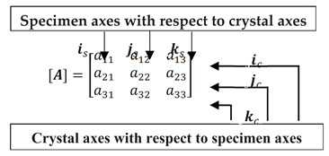
The column vectors of the rotation matrix [A] are the direction cosines of the specimen base axes with respect to the crystal base axes, while the row vectors in [A] are the direction cosines of the crystal base axes with respect to the specimen base axes. Pole figure representation is the stereographic projection of the poles (lattice planes or directions) of the crystals onto the specimen coordinate system, while inverse pole figure is just the opposite, i.e., the projection of the specimen axes onto the crystal coordinate system. Thus, in an inverse pole figure, the projection coordinate system is always the orthonormal coordinate system associated with the crystal, i.e. (). The "poles" to be projected are the specimen axes, e.g., RD, TD, and ND in a rolled specimen. In other words, the column vectors in [A] are used to obtain the inverse pole figure.
Due to crystal symmetry, the choice of the orthonormal coordinate system in the crystal may not be unique, i.e., there may be a number of equivalent coordinate systems that can be selected. For cubic crystal, the number of ways to select the orthonormal coordinate system is 24, while for hexagonal crystal, it is 12. If the specimen axis is projected onto the entire inverse pole figure, i.e., including all the equivalent crystal axes, the inverse pole figure will look the same as pole figure; the only difference is that the projected “poles” are the specimen axes, which have been repeatedly projected multiple times (the number of symmetry operations) onto a number of sets of equivalent orthonormal coordinate systems. Since all these coordinate systems are equivalent, only one of them is needed to perform the projection, which is the standard stereographic triangle (SST) that has been discussed above.
As mentioned before, the column vectors of the orientation matrix are the direction cosines of the three base axes of the specimen with respect to the crystal coordinate system (orthonormal). When plotting inverse pole figures, one of these three base axes is selected, and it is projected onto the crystal coordinate system. Let the coordinates of the selected base axis within the crystal coordinate system be (, , ), where , the stereographically projected coordinates (, ) can then be calculated as:
Within the SST, the projected base axis is identified and represented as a point, which is determined by the crystal orientation (matrix [A]). To represent this point in the IPF map, the color of this point in the SST is used. Clearly, the three color components should be calculated by mapping this point in the SST back to the MCT.
If the SST has been colored using the Miller indices (cubic symmetry only), it is straightforward to directly use the Miller indices (hkl) or [uvw] to calculate the projection coordinates (, ) as the Miller indices are the pole coordinates (normalized) in the unit sphere for stereographic projection (He, 2023; Kittel, 2004). The color of each point in the IPF is calculated using Eq. 3. If the SST has been colored using the extended barycentric coordinates, the color of each point in the SST is defined by the barycentric coordinates. In these two cases, the color mapping is very simple. However, for coloring using the 2nd and 3rd order shape functions, the determination of the color components (or reference coordinates) from the SST is more complicated as the coordinates of each point (x, y) in the SST are to be mapped back to the reference coordinates (color components) using the shape functions, i.e., inverse mapping from the real coordinates to the reference coordinates. Although in the case of 2nd-order shape functions, it is possible to derive an analytical equation to convert the pole coordinates (x, y) to the reference coordinates (, , ), it needs to solve a cubic function. In addition, it has already been shown that the approximated curve side is not exactly the same as the real SST curved side and there are points in the uncovered areas without corresponding reference coordinates. For the mapping using 3rd-order shape functions, the analytical equations describing the inverse mapping are even more complicated and solving them needs numerical methods. Similarly, there are points (uncovered areas) that do not have the corresponding reference coordinates.
To avoid the inverse mapping directly from the SST coordinates to the reference coordinates, in this study, a simple comparison technique is used to identify the color components of any point in the SST. For an arbitrary point in the SST, the color components of the closest node point (of all the approximated points using the shape functions) in the mesh are taken as the color of the point under consideration. The algorithm is very simple: for any point within the SST with known coordinates (x, y), calculate the distance between this point and every node point (color components are known) and find the nearest node. Apparently, it will involve the calculation of the distances between the point and all the node points, which will be computation intensive. Considering the geometries of the SSTs, each SST can be subdivided into smaller regions (Figure 13) and the point under consideration can be first located in one of these regions. Then the closest point is found within this region only. In this way, the computing time needed to search for the closest point can be significantly reduced. The color components of all the points within the SST can be identified unequivocally.
Using the algorithms described above, EBSD data of all crystal symmetries can be represented in IPF maps. A computer program (using the OpenGL graphic library in C++) was written to first convert the Euler angles to orientation matrices using Eq. 24. Then one of the three column vectors of the rotation matrix is taken as the coordinates of the specimen axis with respect to the crystal coordinate system (inverse pole figure), which are used to calculate the projection (x, y) in the IPF. The color of this projection (x, y) is then found and displayed in the IPF map. Figure 14 shows an example of the same EBSD data set (electrical steel, cubic high symmetry) as displayed using different color-coding methods and compared to the IPF map obtained using commercial EBSD software EDAX OIM.
It is seen that the IPF maps (Figure 14b, Figure 14c, and Figure 14d) displayed using the algorithms developed in this study show the same characteristics as that displayed using commercial EBSD software (Figure 14a). Due to the difference in the location of the color centroid of the different algorithms, some of the crystals show apparent differences in color in the maps (see those marked with ovals). Nevertheless, if the color key is accompanied with the IPF map, the representation of the crystal orientations using any of these color-coding algorithms can be used. It is thus demonstrated that using finite element shape functions, it is straightforward to color the standard stereographic triangles to represent orientation data in inverse pole figure mapping. The algorithm presented in this paper can be used to develop customized EBSD software and orientation representation programs for crystal plasticity simulations.
Summary and Conclusions
In this paper, a few coloring algorithms (using Miller indices, barycentric coordinates and finite element shape functions) are compared to color code the SSTs of all crystal symmetries in the 11 Laue groups. The advantages and drawbacks of each algorithm are discussed. These algorithms are then used to display EBSD data in IPF maps. The following conclusions can be drawn:
- Color coding using Miller indices is very simple and straightforward, but it can only be applied to crystals with cubic symmetry since for other symmetries, the color coding will be dependent on the lattice parameters.
- Using extended barycentric coordinates to color the SST is also very simple, but it is only applicable to crystals with high symmetries since those with low symmetries (orthorhombic/tetragonal low and trigonal low) show unfaithful colors at the corners of the curved side.
- Coloring using both second and third order finite element shape functions by mapping from the Maxwell color triangle to the SSTs provides a robust method for color coding; both can be used in IPF mapping.
- The use of third-order shape functions results in much better accuracy in approximating the curved side of the SSTs than that using second-order shape functions, leading to more accurate coloring; this is the preferred method for IPF mapping.
- The color centroid of the SSTs color coded using third-order shape functions can be adjusted using a distance factor, which can conveniently move the color centroid close to the geometric centroid of the SSTs.
- The IPF maps displayed using the developed algorithms show the same characteristics as that displayed using commercial EBSD software; only small differences in color are noticed in some crystals due to the difference in the location of the color centroid.
- The algorithms presented in this study can be used to develop customized EBSD software and to develop orientation representation program for crystal plasticity simulations.
References
- Adams, B. L.; Wright, S. I.; Kunze, K. Orientation imaging: The emergence of a new microscopy. Metallurgical Transactions A 1993, 24(4), 819–831. [Google Scholar] [CrossRef]
- AMETEK Inc., 2019. EDAX OIM Analysis Software Manual. Pleasanton, California: EDAX OIM.
- Bunge, H. J. Texture Analysis in Materials Science: Mathematical Methods; Butterworth-Heinemann: Oxford, 1982. [Google Scholar]
- Dingley, D. J.; Randle, V. Microtexture determination by electron back-scatter diffraction. Journal of Materials Science 1992, 27(17), 4545–4566. [Google Scholar] [CrossRef]
- He, Y. Stereographic Projection of Theoretical Orientation Relationships Between Crystals of Any Types in Phase Transformation and Precipitation. Crystal Research and Technology 2023, 59(1), 2300242(1-15). [Google Scholar] [CrossRef]
- Kittel, C. Introduction to Solid State Physics, 8th ed; John Wiley & Sons, Inc.: Hoboken, 2004. [Google Scholar]
- Miller, W. H. A Treatise on Crystallography; Cambridge Press: London, 1939. [Google Scholar]
- Mobius, A. F., 1885. Der barycentrische Calcul. In: Baltzer, Richard, ed., August Ferdinand Möbius Gesammelte Werke. s.l.:Leipzig: S. Hirzel, p. 1–388.
- Nolze, G.; Hielscher, R. Orientations – perfectly colored. Journal of Applied Crystallography 2015, 49, 1786–1802. [Google Scholar] [CrossRef]
- Oxford Instruments. HKL Channel 5 Manual; Oxford Instruments: Witney, Oxon, UK, 2009. [Google Scholar]
- Randle, V.; Engler, O. Introduction to texture analysis: macrotexture, microtexture and orientation mapping; CRC Press: Boca Raton, Florida, 2000. [Google Scholar]
- Whittaker, E. J. W. Crystallography: an Introduction for Earth Science (and Other Solid State) Students; Pergamon: Oxford, 1981. [Google Scholar]
- Wright, S. I.; Zhao, J. W.; Adams, B. L. Automated Determination of Lattice Orientation From Electron Backscattered Kikuchi Diffraction Patterns. Texture, Stress, and Microstructure 1991, 13(2-3), 123–131. [Google Scholar] [CrossRef]
- Wright, W. D. The Measurement of Color; Adam Hilger Limited: London, 1969. [Google Scholar]
- Zienkiewicz, O. C.; Taylor, R. L.; Zhu, J. Z. Finite Element Method - Its Basis and Fundamentals (6th Edition); Elsevier: London, 2005. [Google Scholar]
Figure 1.
The 7 different shapes of the SSTs for the 11 Laue groups: (a) 5 sectors of a unit circle for symmetries other than cubic, (b) portions of a 45°-sector for cubic low and cubic high symmetries, (c) the coordinates of the vertices for the 5 sectors as defined on a unit circle centered at (0,0), (d) the coordinates of the vertices for the cubic low and cubic high symmetries. Note that each SST can be drawn with the first straight side starting at 0° and the other straight side ending at the sector angle (θ = 30°, 45°, 60°, 90° and 120°).
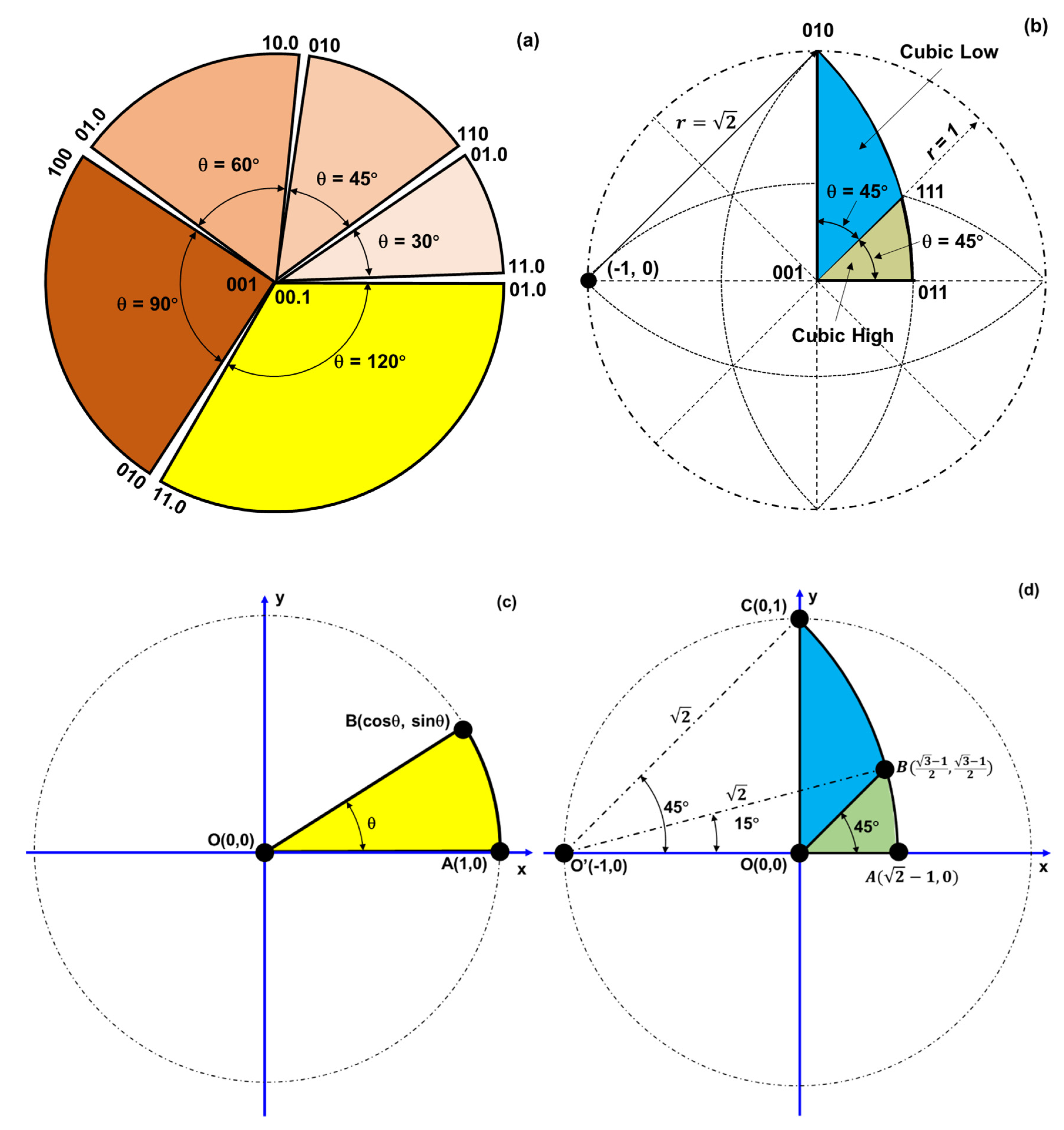
Figure 2.
The increase of the number of poles in the SST of cubic crystals (m3m) when the maximum integer (m) of the Miller indices {hkl} is increased: (a) m = 9, (b) m = 12, (c) m = 15. .
Figure 2.
The increase of the number of poles in the SST of cubic crystals (m3m) when the maximum integer (m) of the Miller indices {hkl} is increased: (a) m = 9, (b) m = 12, (c) m = 15. .
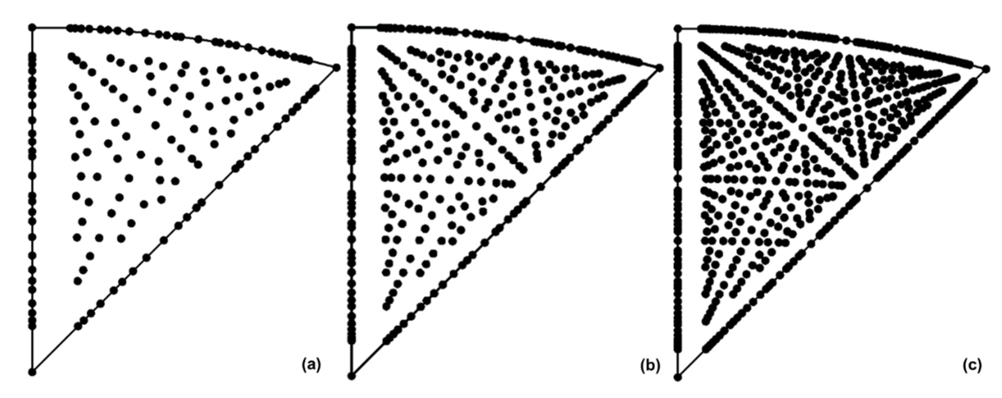
Figure 3.
Color coding of the SST of cubic crystals (m3m) using Miller indices: (a) color key of the commercial software EDAX OIM, (b) labels of the poles in the SST with a maximum integer of m = 6, (c) color-coded SST using Miller indices (Eq. 3). Note the difference in the location of the center (white) between (a) and (c).
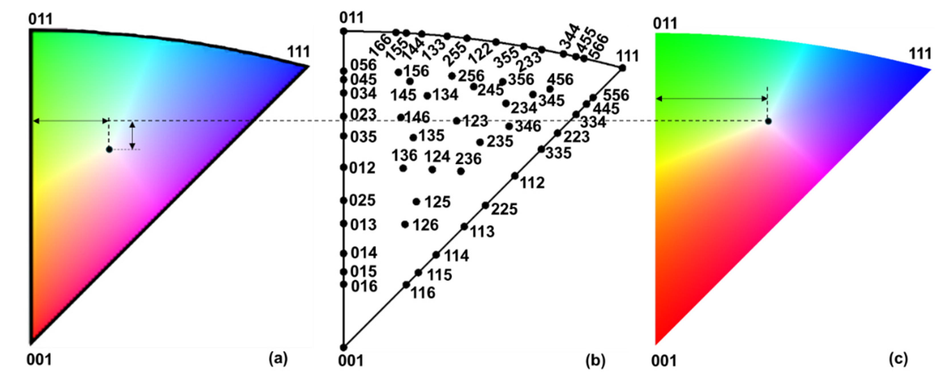
Figure 4.
The MCT and the coloring of arbitrary triangles: (a) the MCT (equilateral), (b) discretization (n = 10) of the MCT to obtain the reference coordinates and the color components, (c) the areal coordinates of a point within an arbitrary triangle, (d) the colored points in an arbitrary triangle using their areal coordinates. .
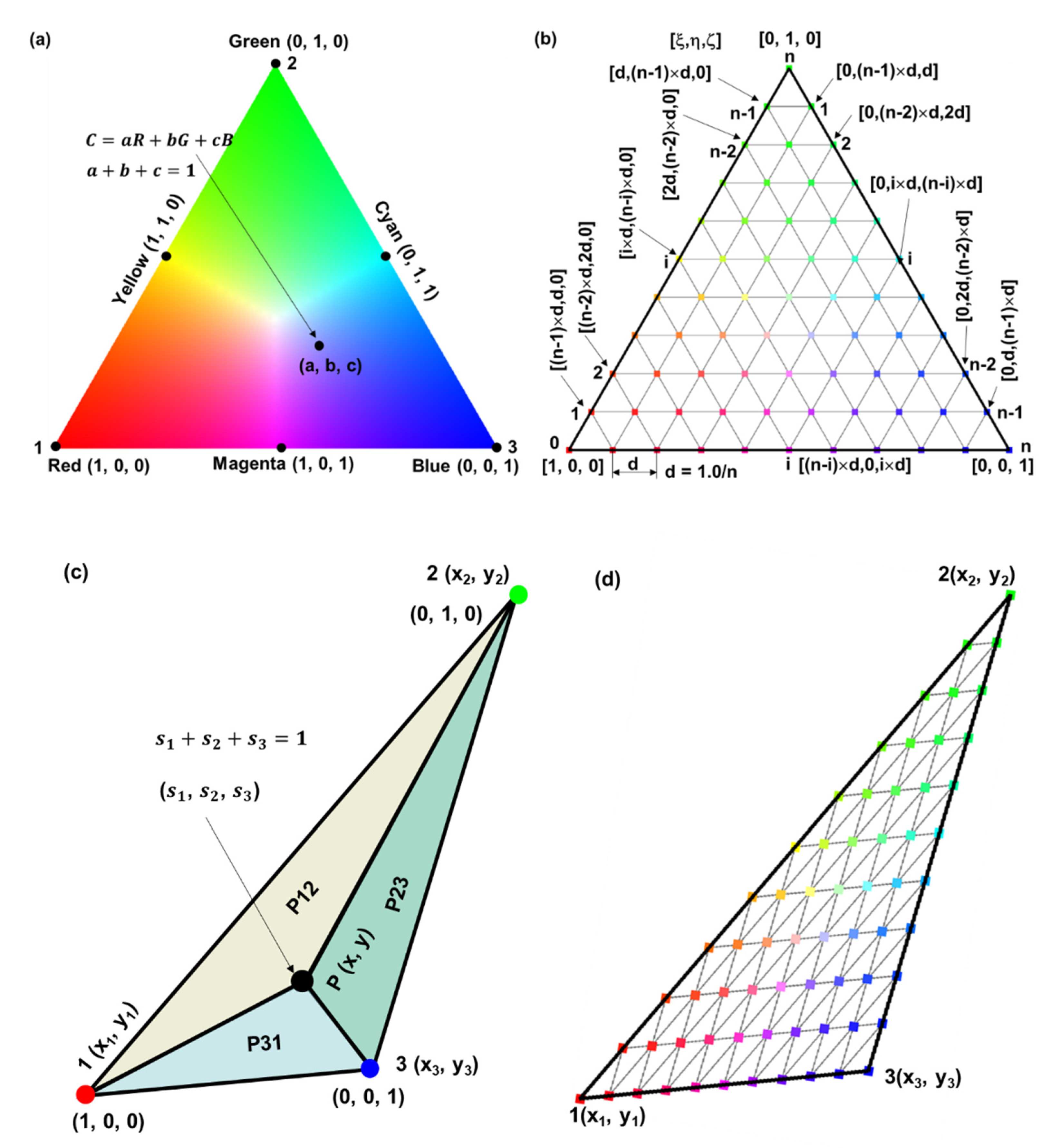
Figure 5.
Color-coded SSTs using generalized barycentric coordinates for crystals with different symmetries: (a) cubic low, (b) cubic high, (c) hexagonal high, (d) tetragonal high, (e) trigonal/hexagonal low, (f) orthorhombic/tetragonal low, (g) trigonal low.
Figure 5.
Color-coded SSTs using generalized barycentric coordinates for crystals with different symmetries: (a) cubic low, (b) cubic high, (c) hexagonal high, (d) tetragonal high, (e) trigonal/hexagonal low, (f) orthorhombic/tetragonal low, (g) trigonal low.
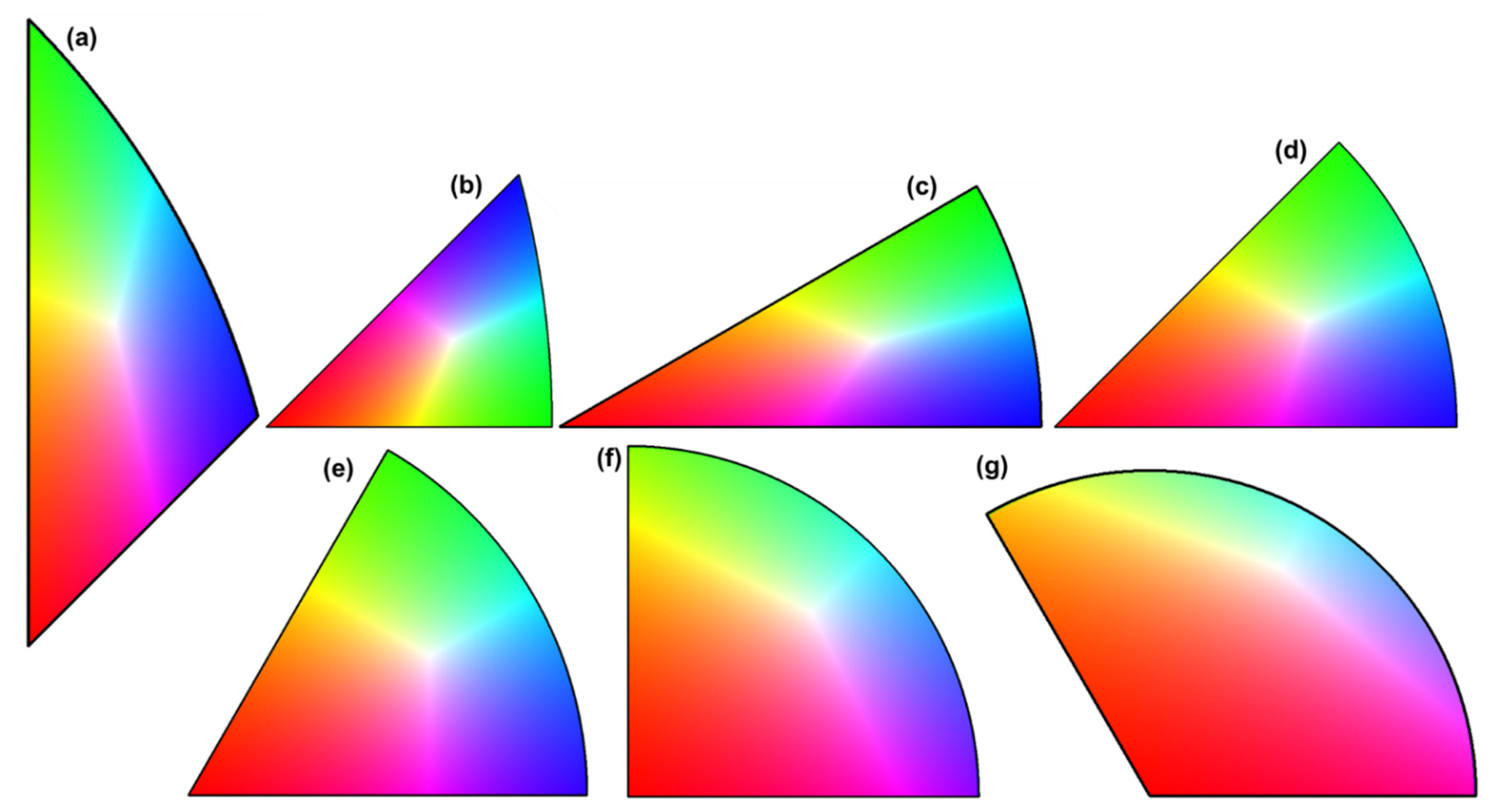
Figure 6.
Mapping from the MCT to SSTs using linear interpolation (partial coloring): (a) cubic low symmetry, (b) cubic high symmetry, (c) hexagonal low symmetry.
Figure 6.
Mapping from the MCT to SSTs using linear interpolation (partial coloring): (a) cubic low symmetry, (b) cubic high symmetry, (c) hexagonal low symmetry.
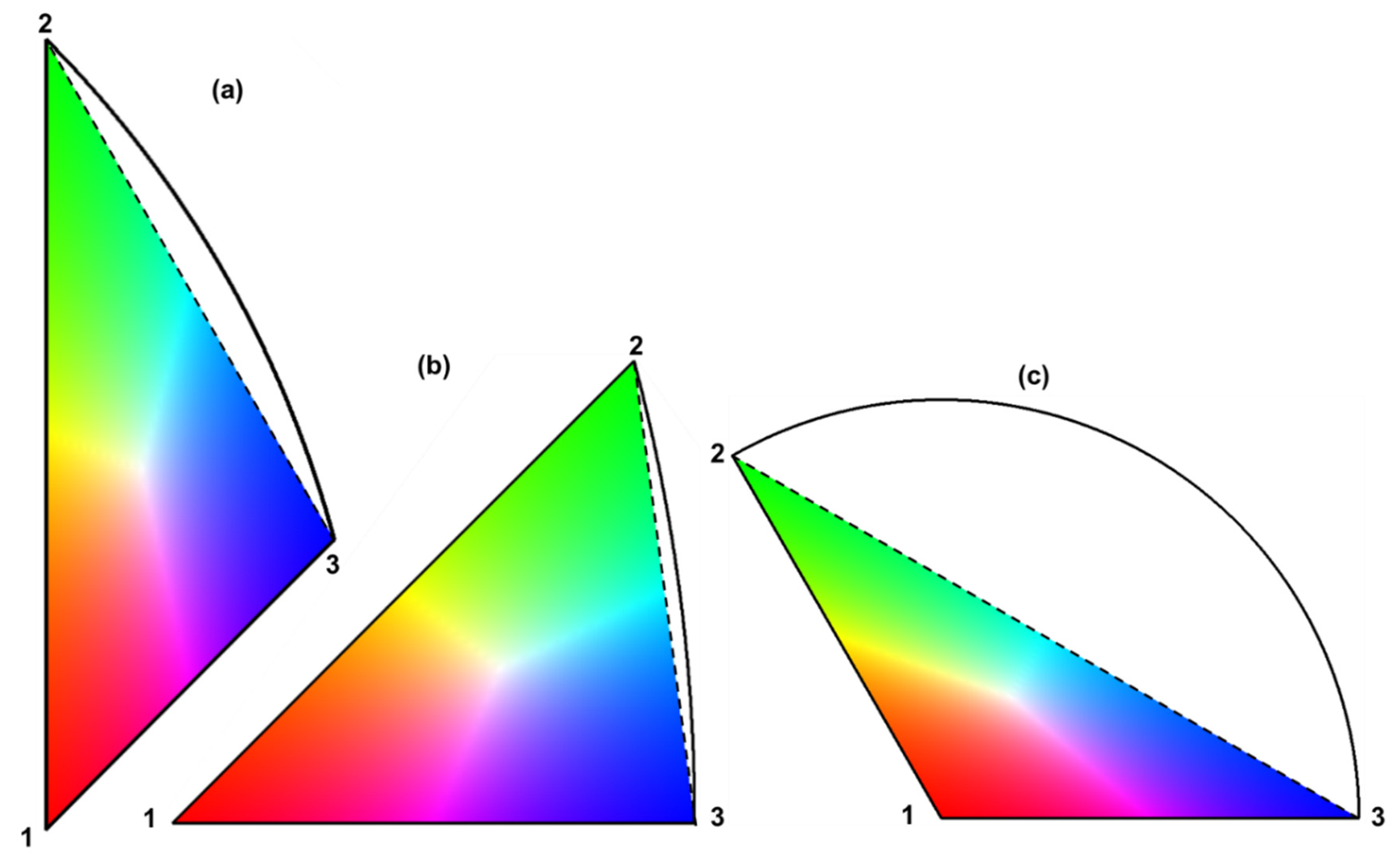
Figure 7.
The additional points needed to approximate the SSTs using second- and third- order shape functions: (a), (d) SSTs for tetragonal symmetry, (b), (e) SST for cubic low symmetry, (c), (f) SST for cubic high symmetry. (a), (b), (c) are for second-order shape functions, (d), (e), (f) are for third-order shape functions.
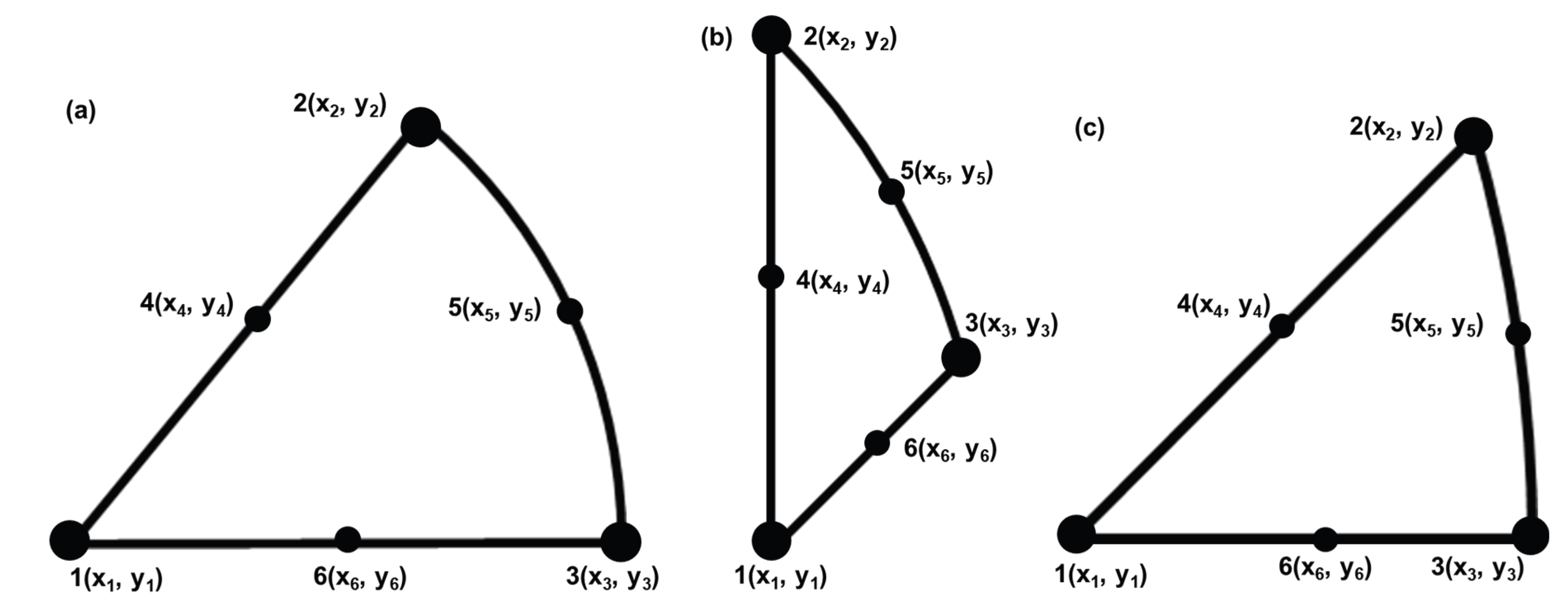
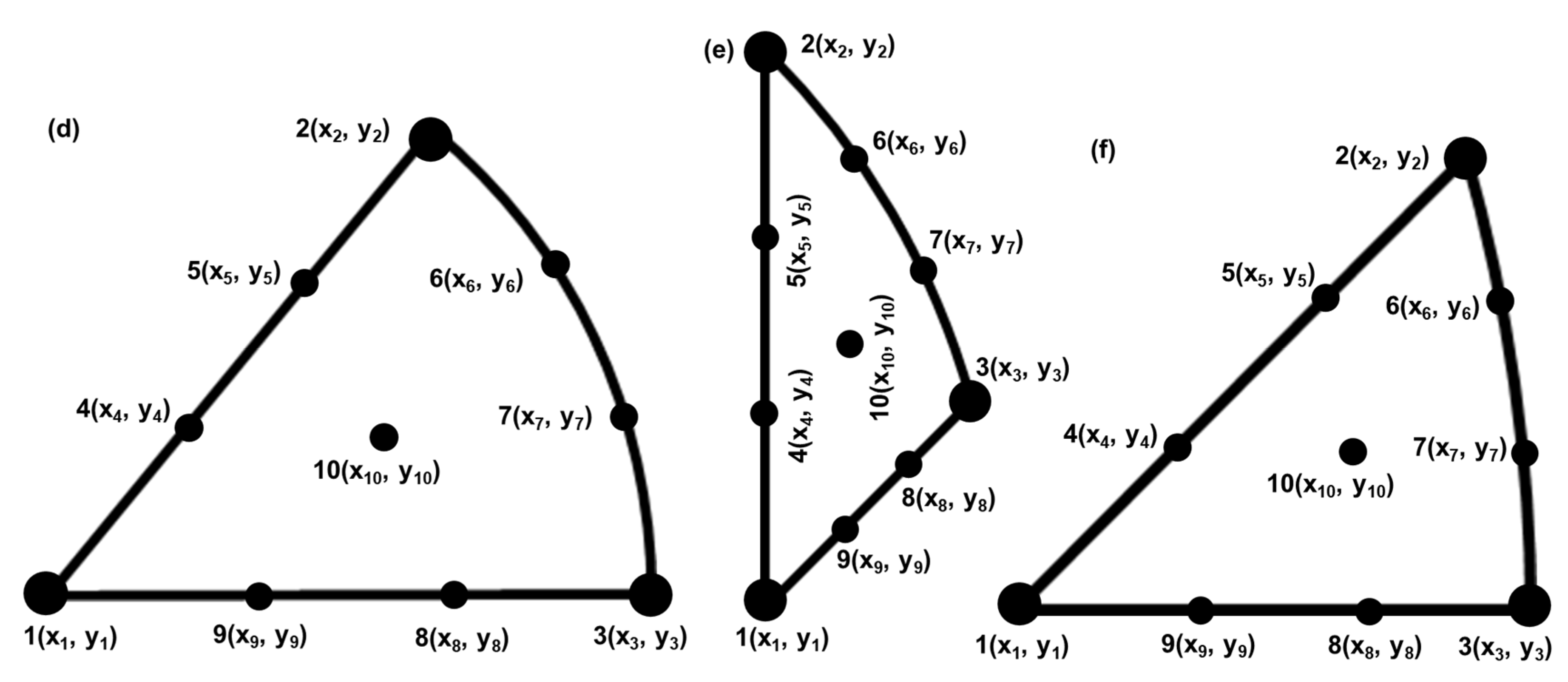
Figure 8.
Color-coded SSTs using second-order shape functions for crystals with different symmetries: (a) cubic low, (b) cubic high, (c) hexagonal high, (d) tetragonal high, (e) trigonal/hexagonal low, (f) orthorhombic/tetragonal low, (g) trigonal low. Note the uncolored portions in (f) and (g).
Figure 8.
Color-coded SSTs using second-order shape functions for crystals with different symmetries: (a) cubic low, (b) cubic high, (c) hexagonal high, (d) tetragonal high, (e) trigonal/hexagonal low, (f) orthorhombic/tetragonal low, (g) trigonal low. Note the uncolored portions in (f) and (g).
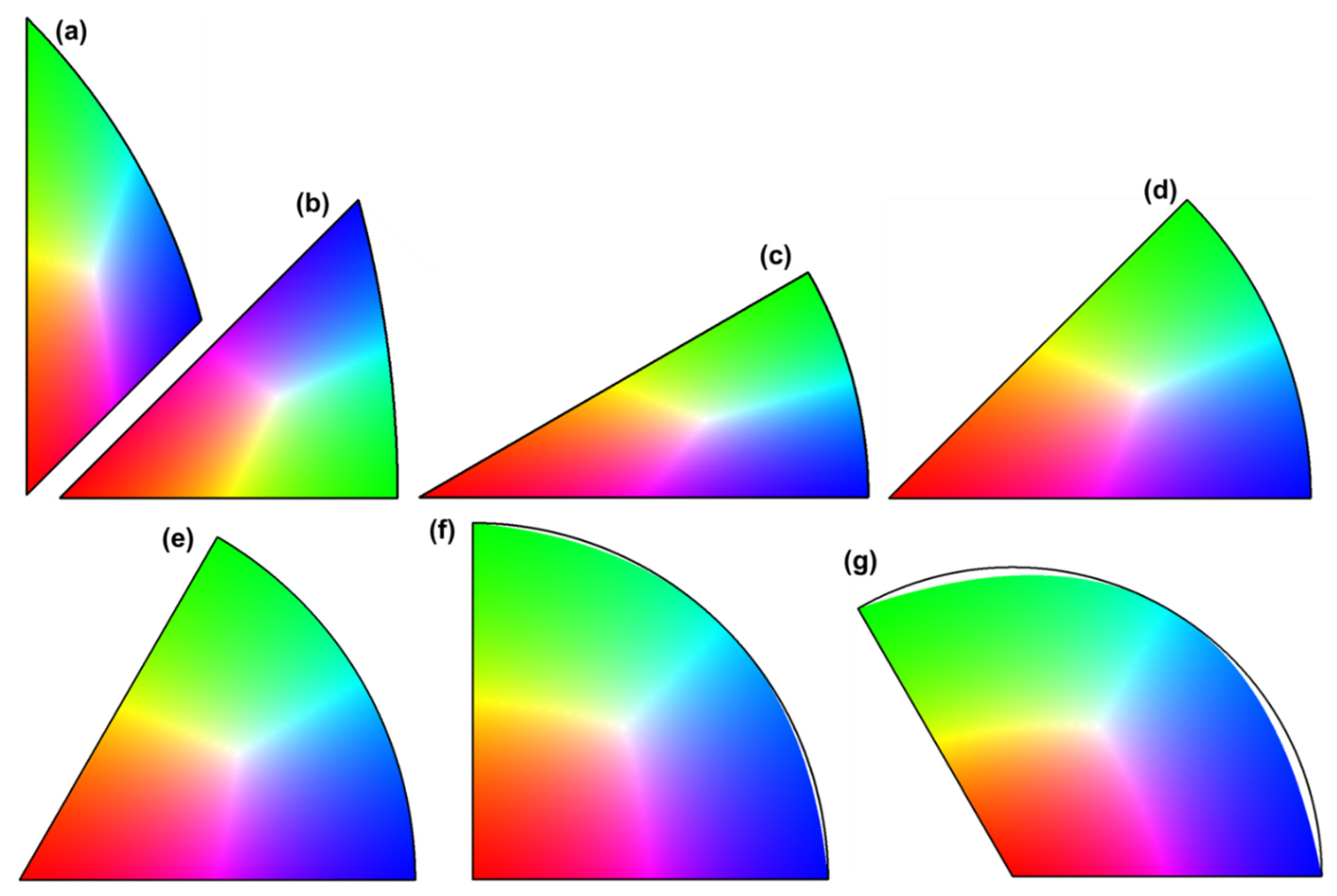
Figure 9.
Color-coded SSTs using third-order shape functions for crystals with different symmetries: (a) cubic low, (b) cubic high, (c) hexagonal high, (d) tetragonal high, (e) trigonal/hexagonal low, (f) orthorhombic/tetragonal low, (g) trigonal low. Note that in this case (f) and (g) are almost completely colored.
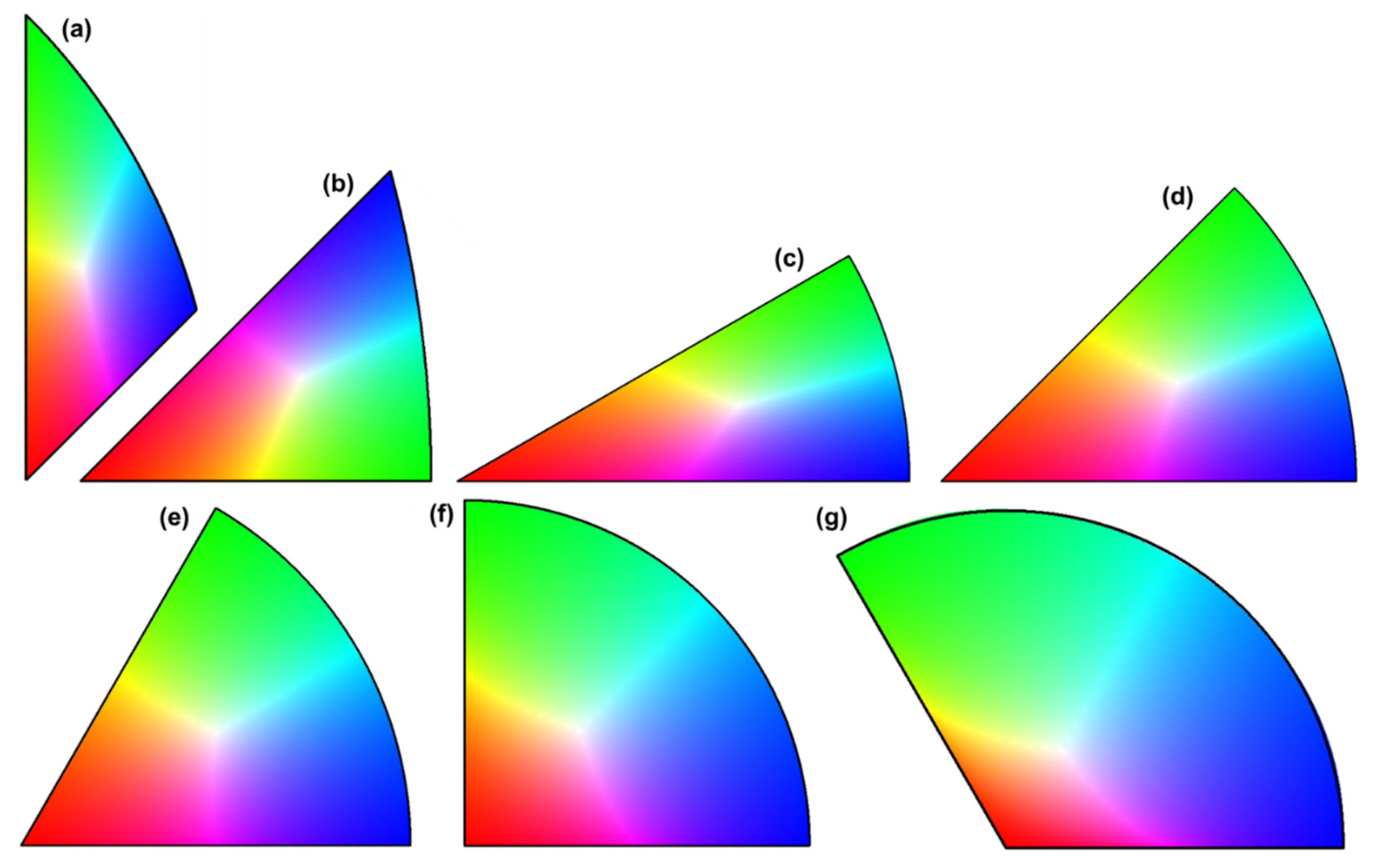
Figure 10.
Coloring the curved side of the SST of the hexagonal low symmetry using 2nd-order shape functions: (a) discretizing the SST using nodes mapped from the MCT (leaving two uncovered areas), (b) using the points on the curved side to replace the nodes mapped from the reference coordinates with = 0, (c) the completely colored SST.
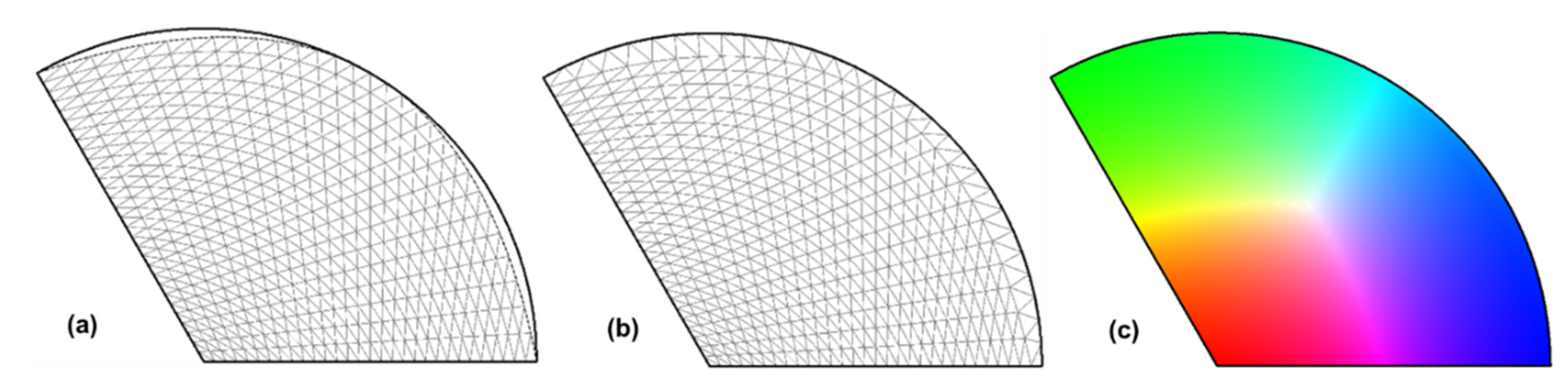
Figure 11.
Effect of the distance factor on the color centroid of the SSTs for: (a)-(c) orthorhombic symmetry, (d)-(f) trigonal low symmetry.
Figure 11.
Effect of the distance factor on the color centroid of the SSTs for: (a)-(c) orthorhombic symmetry, (d)-(f) trigonal low symmetry.
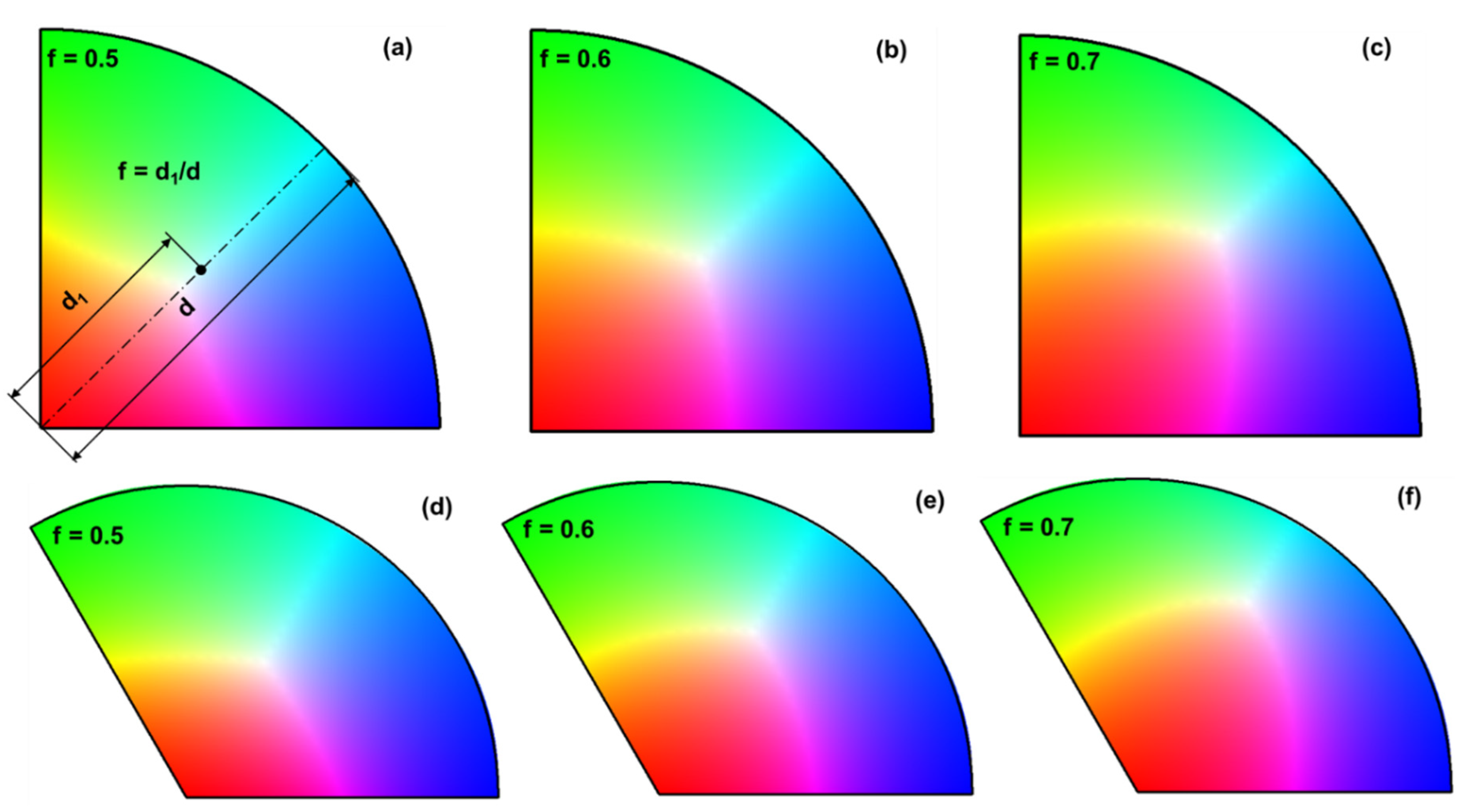
Figure 12.
Effect of the number of divisions in MCT on the area difference between the real and mapped SSTs: (a) second-order shape functions, (b) third-order shape functions.
Figure 12.
Effect of the number of divisions in MCT on the area difference between the real and mapped SSTs: (a) second-order shape functions, (b) third-order shape functions.
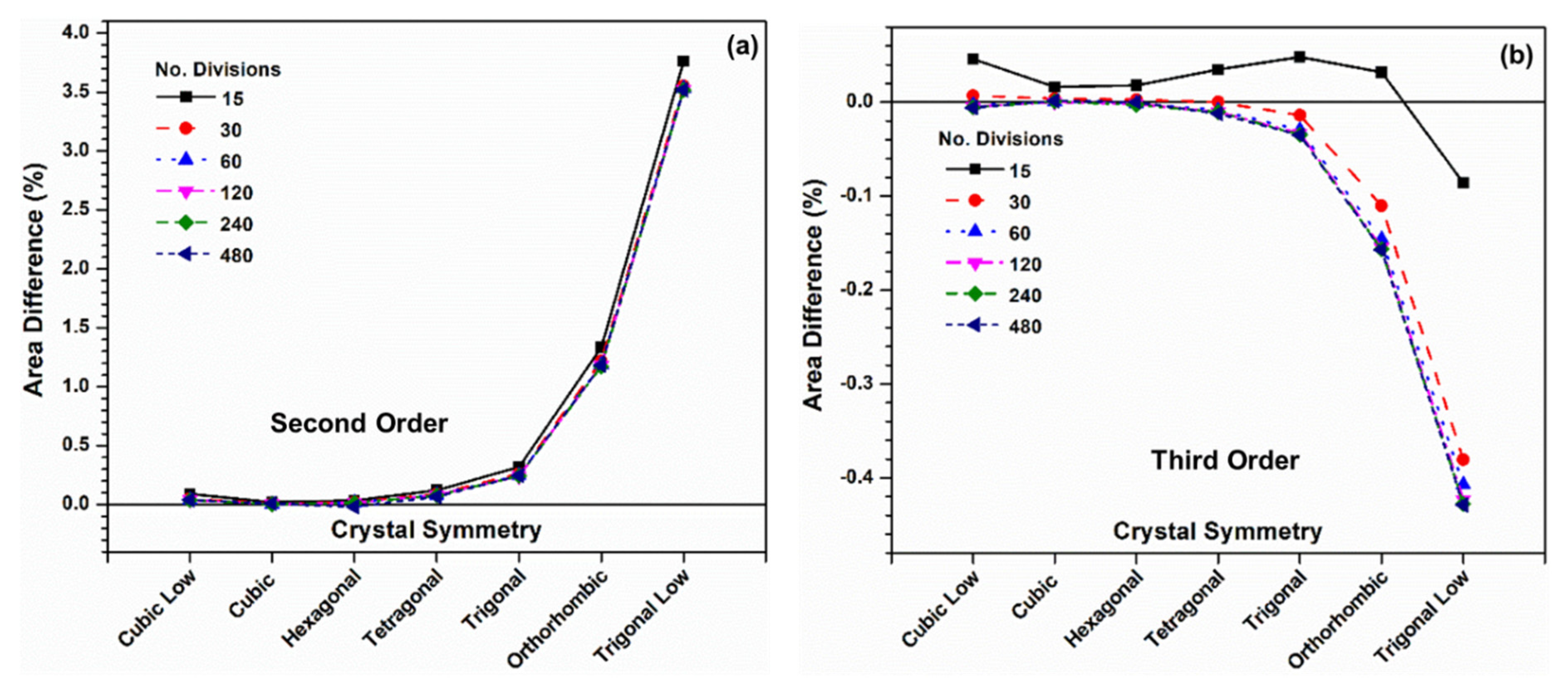
Figure 13.
Dividing the SSTs into regions for the convenience of finding the color components of an arbitrary point: (a) SST with tetragonal symmetry, (b) SST with cubic low symmetry, (c) SST with cubic high symmetry.
Figure 13.
Dividing the SSTs into regions for the convenience of finding the color components of an arbitrary point: (a) SST with tetragonal symmetry, (b) SST with cubic low symmetry, (c) SST with cubic high symmetry.
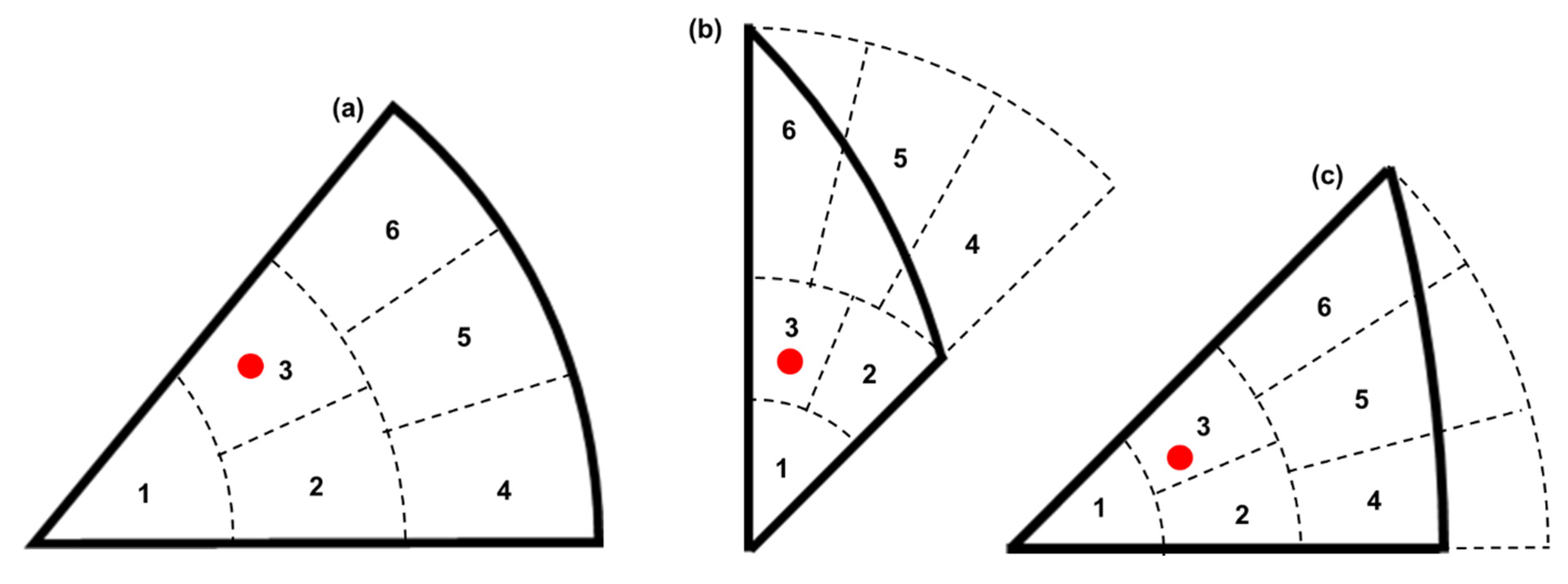
Figure 14.
IPF maps of the same EBSD data set displayed using different color-coding algorithms: (a) EDAX OIM, (b) Miller indices, (c) second-order shape functions, (d) third-order shape functions.
Figure 14.
IPF maps of the same EBSD data set displayed using different color-coding algorithms: (a) EDAX OIM, (b) Miller indices, (c) second-order shape functions, (d) third-order shape functions.
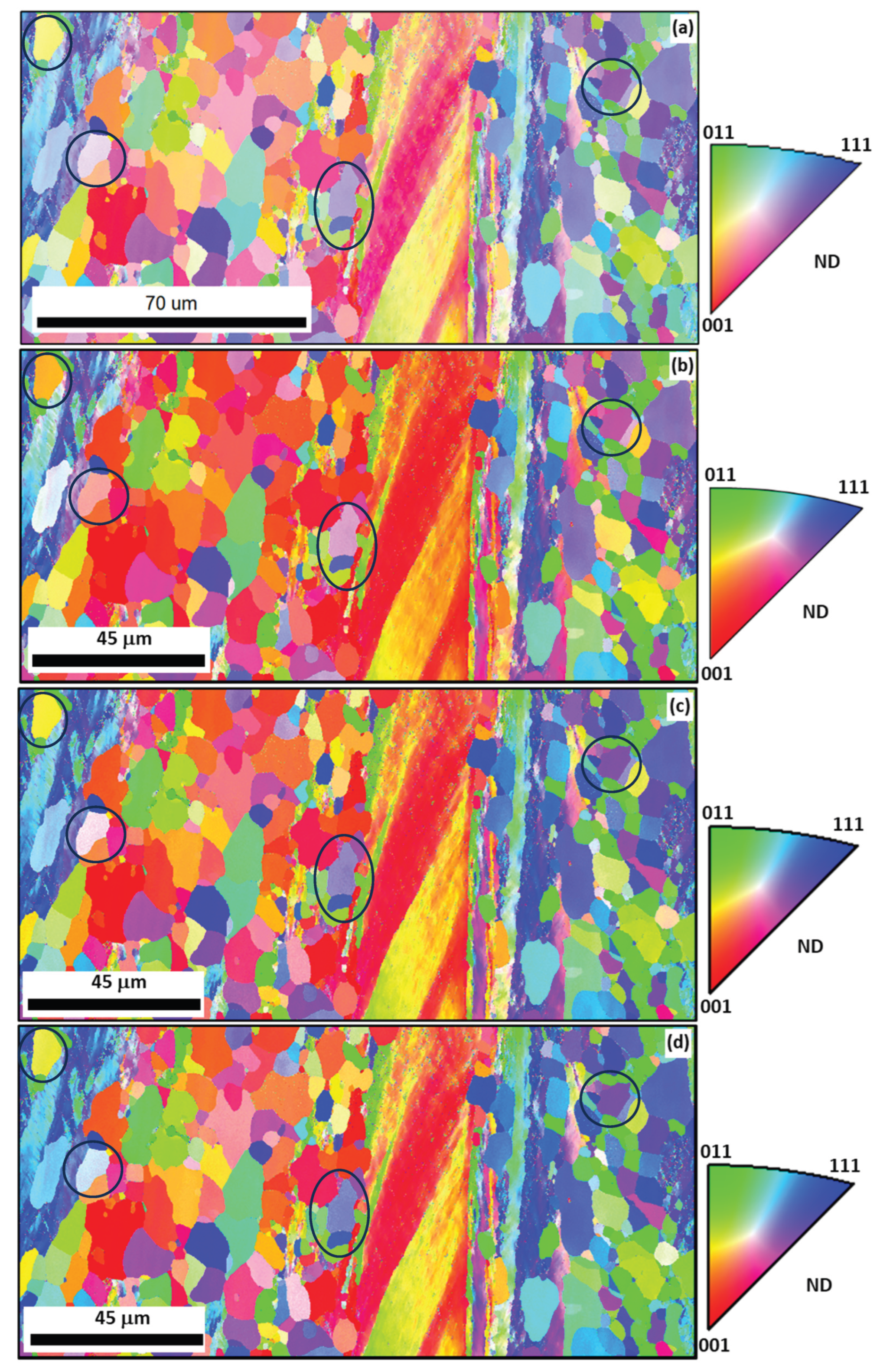

Table 1.
The mapped SST areas and the area difference between the real SST and the mapped one using different orders of shape functions.
Table 1.
The mapped SST areas and the area difference between the real SST and the mapped one using different orders of shape functions.
| Shape Function Order | Crystal Symmetry | ||||||
|---|---|---|---|---|---|---|---|
| Cubic Low | Cubic | Hexa-gonal | Tetra-gonal | Trigonal | Ortho-rhombic | Trigonal Low | |
| SST Area | 0.206611 | 0.078787 | 0.261799 | 0.392699 | 0.523599 | 0.785398 | 1.0472 |
| 1st | 0.183017 | 0.075807 | 0.249993 | 0.353546 | 0.433016 | 0.499985 | 0.433016 |
| ΔA (%) | 11.42 | 3.78 | 4.51 | 9.97 | 17.30 | 36.34 | 58.65 |
| 2nd | 0.206524 | 0.078783 | 0.261755 | 0.392381 | 0.522305 | 0.776065 | 1.0102 |
| ΔA (%) | 0.0423 | 0.0043 | 0.0168 | 0.0810 | 0.2471 | 1.1884 | 3.5327 |
| 3rd | 0.206617 | 0.078786 | 0.261802 | 0.392732 | 0.523753 | 0.786542 | 1.05146 |
| ΔA (%) | -0.0026 | 0.0006 | -0.00097 | -0.0084 | -0.0295 | -0.1456 | -0.4073 |
The number of divisions on each side for discretization is 60. ΔA = (SST Area – Mapped Area)/ SST Area ×100. Note Cubic = Cubic High, Hexagonal = Hexagonal High, Tetragonal = Tetragonal High, Trigonal = Trigonal High.
Disclaimer/Publisher’s Note: The statements, opinions and data contained in all publications are solely those of the individual author(s) and contributor(s) and not of MDPI and/or the editor(s). MDPI and/or the editor(s) disclaim responsibility for any injury to people or property resulting from any ideas, methods, instructions or products referred to in the content. |
© 2025 by the author. Licensee MDPI, Basel, Switzerland. This article is an open access article distributed under the terms and conditions of the Creative Commons Attribution (CC BY) license (https://creativecommons.org/licenses/by/4.0/).
Copyright: This open access article is published under a Creative Commons CC BY 4.0 license, which permit the free download, distribution, and reuse, provided that the author and preprint are cited in any reuse.


