
Submitted:
15 October 2025
Posted:
15 October 2025
You are already at the latest version
Abstract
This article explores the foundational mechanisms of the Discrete Event System Specification (DEVS) theory—closure under coupling, universality, and uniqueness—and their critical role in enabling interoperability through modular, hierarchical simulation frameworks. Closure under coupling empowers modelers to compose interconnected models, both atomic and coupled, into unified systems without departing from the DEVS formalism. We show how this modular approach supports the scalable and flexible construction of complex simulation architectures on a firm system-theoretic foundation. Also, we show that facilitating the transformation from non-modular to modular and hierarchical structures endows a major benefit in that existing non-modular models can be accommodated by simply wrapping them in DEVS-compliant format. Therefore, DEVS theory simplifies model maintenance, integration, and extension, thereby promoting interoperability and reuse. Additionally, we demonstrate how DEVS universality and uniqueness guarantee that any system with discrete event interfaces can be structurally represented with the DEVS formalism, ensuring consistency across heterogeneous platforms. We propose that these mechanisms collectively can streamline simulator design and implementation for advancing simulation interoperability. Finally, we conclude by discussing how DEVS concepts apply to the Department of Defense’s Modular Open Systems Approach (MOSA) to deployment of software systems. We propose that the DEVS-based development of modeling and simulation architecture provides a rigorous, formal basis to uniformly and efficiently integrate, execute, and manage diverse software systems, thereby enhancing interoperability, scalability, and maintainability across Department of Defense (DoD) software initiatives.
Keywords:
DEVS discrete event system specification
; closure under coupling
; hierarchical modular construction
; interoperability
; flattening
; non-modular system
; system entity structure
; MOSA
; modular open system approach
; modeling and simulation
; FMI functional mock-up interface
1. Introduction
DEVS (Discrete Event System Specification) theory provides foundational mechanisms —closure under coupling, universality, and uniqueness — enabling interoperability through modular, hierarchical model construction and simulation [1,2,3,4,5]. Although the foundational mechanisms of DEVS have been discussed in several publications [6,7,8,9,10,11,12,13,14,15,16,17], our aim is to provide a more intuitive understanding of the concept that will help extend the concept to broader contexts of simulation interoperability and development of software systems within DoD’s Modular Open Systems Approach (MOSA)[18]. Closure under coupling in DEVS ensures that interconnected models, whether atomic or coupled, can be composed into a single unified model without leaving the formal DEVS framework. This modularity enables the construction of complex, hierarchical systems from simpler, reusable components streamlining model management and supporting scalability [6,16,19,20,21,22,23]. In current practice, however, simulation systems are often developed without regard to modular construction considerations. This motivates the upcoming discussion of transformation from non-modular to modular and hierarchical structures which makes models easier to maintain, integrate, and expand, thus promoting interoperability and reuse.
DEVS universality and the uniqueness of representation [24,25,26,27,28] guarantee that any system characterized by discrete event interfaces and behaviors can be accurately modeled and executed within the DEVS framework. We will review these concepts in the context that they provide a common formal basis for representing diverse systems, enabling uniform treatment and integration of models, regardless of complexity or origin. This is crucial for implementations that require consistent, reliable integration across heterogeneous platforms. Flattening and hierarchical organization [2,5,29,30,31,32,33,34,35,36,37] in DEVS allow nested models to be represented and executed as atomic models, preserving behavioral equivalence. We will review these operations and provide simplified approach to using them to facilitate efficient DEVS simulation execution. of representation.
Figure 1 sketches the types of DEVS models and a taxonomy of DEVS models and is intended to help present the organization of the paper. In the sequel, this paper is organized as follows:
Section 2 reviews the modeling and simulation (M&S) framework developed in reference [17] to place the breakdown of DEVS models into Atomic and Coupled (Figure 1) in the wider context of the M&S enterprise. It goes on to provide background information on DEVS universality and uniqueness of representation which, along with closure under coupling, provide theoretical support for claiming that DEVS supports the best way to construct simulation models for interoperability and related traits. Finally, it provides background information on the closure under coupling and its foundation for definition of the DEVS abstract simulator/simulation protocol. to place the breakdown of DEVS models into Atomic and Coupled (Figure 1) in the wider context of the M&S enterprise. It goes on to provide background information on DEVS universality and uniqueness of representation which, along with closure under coupling, provide theoretical support for claiming that DEVS supports the best way to construct simulation models for interoperability and related traits. Finally, it provides background information on the closure under coupling and its foundation for definition of the DEVS abstract simulator/simulation protocol.
Section 3 reviews the DEVS Simulation Protocol and Abstract Simulator and builds on this background to present a new design for object-oriented implementation of DEVS Abstract Simulator. The design employs closure under coupling explicitly to simplify the operation of the DEVS simulator.
Section 4 reviews the DEVS Bus concept for generalizing the DEVS protocol to apply more generally. It then goes on to consider the inter-conversion between non-modular and modular form for flat coupled models (Figure 1).
This finding has important implications for distributed simulations in practice, since it indicates that existing federations of various types can be coordinated within the same coupled model without needing to refactor their internal structures. This removes a major barrier to widespread adoption of DEVS within organizations with large legacy simulation investments.
Section 5 discusses operations on the hierarchical structure of DEVS models flattening and its inverse deepening. In the flattening process hierarchical coupled models are transformed to behaviorally equivalent “flat” coupled models, i.e.; having only atomic models as components [31,38,39,40]. Conversely, as suggested in Figure 1, the reverse direction is also possible – “deepening” adds hierarchical structure to flat coupled models. This section concludes with the implications for structural operations for the design of DEVS models and simulators. In summary, flattening eliminates structure by reducing message traffic and increasing simulation efficiency; Deepening can introduce hierarchical structure to enable modularity, reuse, and scalability. [14,54] 230,274. Conversely, as suggested in Figure 1, the reverse direction is also possible – “deepening” adds hierarchical structure to flat coupled models. This section concludes with the implications for structural operations for the design of DEVS models and simulators.
Section 6 considers DEVS closure under coupling in relation to closure properties in other systems-adjacent formalisms so that the special nature of the DEVS concept is highlighted.
Section 7 serves as Discussion and Summary section in placing the hierarchical modular features of DEVS models in application to DoD’s MOSA with a view toward providing a foundation for the modular construction it seeks. Moreover, the application of DEVS theory within Model Based System Engineering (MBSE) and Mathematical Systems Theory offers potential concepts and tools to enable formal analysis of complex MOSA designs within DoD.
Finally, Section 8 concludes the paper with discussion of limitations and opportunities for further development.
Several appendices provide detail for the interested reader.
2. Background: Modeling and Simulation Framework and DEVS Theory
The Modeling and Simulation Framework, Figure 2 a), formalizes a small set of foundational entities and relationships that describe any model–simulation system in an abstract, domain-independent way. This framework provides the conceptual scaffolding behind DEVS and other system-specifications [17,31,38,39,40]. In brief the entities are a) Source System, a real or imagined system, characterized by observable behaviors over time in a defined set of variables; it may be physical (a spacecraft), conceptual (a policy process), or hypothetical. b) Experimental Frame (EF), a specification of the conditions under which the system is observed or experimented upon, includes: inputs: allowable stimuli, Outputs: observations to record, Conditions: intended scope, constraints, metrics, sampling plans (in collaborative modeling, the EF ensures reproducibility and relevance), c) Model, an abstract, formal specification that generates behaviors consistent with the source system under the EF, exists in many forms: mathematical equations, logical rules, state machines, must be valid with respect to the EF (i.e.; produce correct behavior for the intended scope), d) Simulator, the computational realization that executes the model to produce behavior over (simulated) time, separates model specification from execution engine, allowing reuse and platform independence. The entities are related by a) the validity relation that judges whether the model represents the system’s behavior under the EF, b) the simulator realizes (executes) the model correctly. In summary, executing the simulator of the model produces observable behavior for analysis and validation against the real system within the EF entities and relationships that describe any model–simulation system in an abstract, domain-independent way. This framework provides the conceptual scaffolding behind DEVS and other system-specifications [13,41,42]. In brief the entities are a) Source System, a real or imagined system, characterized by observable behaviors over time in a defined set of variables; it may be physical (a spacecraft), conceptual (a policy process), or hypothetical. b) Experimental Frame (EF), a specification of the conditions under which the system is observed or experimented upon, includes: inputs: allowable stimuli, Outputs: observations to record, Conditions: intended scope, constraints, metrics, sampling plans (in collaborative modeling, the EF ensures reproducibility and relevance), c) Model, an abstract, formal specification that generates behaviors consistent with the source system under the EF, exists in many forms: mathematical equations, logical rules, state machines, must be valid with respect to the EF (i.e.; produce correct behavior for the intended scope), d) Simulator, the computational realization that executes the model to produce behavior over (simulated) time, separates model specification from execution engine, allowing reuse and platform independence. The entities are related by a) the validity relation that judges whether the model represents the system’s behavior under the EF, b) the simulator realizes (executes) the model correctly. In summary, executing the simulator of the model produces observable behavior for analysis and validation against the real system within the EF.
Figure 2 b) provides more structuring of the Experimental Frame, as a coupled model consisting of 1) generators of inputs to the system or model, 2) acceptors that check the constraints and conditions governing termination of execution, and 3) transducers that process raw simulation data to provide metrics and summaries of interest with the frame. More details are available in [13,41,42].
2.1. DEVS Universality and Uniqueness
We first briefly recall the ability of DEVS to represent general dynamic systems; for a more introductory and detailed presentation see [17]. In the DEVS formalism, atomic models keep track of how long it has been in its current state. That duration—called the elapsed time—is a core input to handling both internal scheduling and reacting to external inputs. By feeding elapsed time into the state-update logic, a DEVS model can faithfully reproduce continuous dynamics within a discrete-event framework. The model maintains its representation of the system state, as well as the elapsed time since its last update of this state. When an input arrives, the model updates the continuous variables over the elapsed time before applying the input and resetting the elapsed time variable to 0. This ensures the state reflects all continuous evolution up to the instant of the external event. To model continuous-time systems described by differential equations, DEVS employs elapsed time to integrate state derivatives between events. This on demand integration avoids fixed time-step loops, advancing state only when inputs arrive or outputs are needed. In the DEVS formalism, atomic models keep track of how long it has been in its current state. That duration—called the elapsed time—is a core input to handling both internal scheduling and reacting to external inputs. By feeding elapsed time into the state-update logic, a DEVS model can faithfully reproduce continuous dynamics within a discrete-event framework. The model maintains its representation of the system state, as well as the elapsed time since its last update of this state. When an input arrives, the model updates the continuous variables over the elapsed time before applying the input and resetting the elapsed time variable to 0. This ensures the state reflects all continuous evolution up to the instant of the external event. To model continuous-time systems described by differential equations, DEVS employs elapsed time to integrate state derivatives between events.
Such a representation is an instance of general systems that have discrete event input/output interfaces. As depicted in Figure 3 a) we consider the representation of DEVS-like systems, defined as systems with input and output time segments that contain events that happen at discrete points in time. These differ from continuous time segments with variable values defined throughout the interval. As shown in Figure 3 b), the considerations begin with the lowest level of the system specification hierarchy and works up to the highest level in stages: the IORO (input/output relation), IOFO (input/output function), Canonical I/O System (state level) and Coupled System. In these terms, DEVS representation of DEVS-like systems is universal (applies to all such systems at the IORO level) and unique (their minimal state representations are isomorphic to DEVS systems at the state level). DEVS representation at the Coupled System level is characterized by its ability to support efficient component-wise simulation of multi-component systems [17]. As depicted in Figure 3 a) we consider the representation of DEVS-like systems, defined as systems with input and output time segments that contain events that happen at discrete points in time. These differ from continuous time segments with variable values defined throughout the interval. As shown in Figure 3 b), the considerations begin with the lowest level of the system specification hierarchy and works up to the highest level in stages: the IORO (input/output relation), IOFO (input/output function), Canonical I/O System (state level) and Coupled System. In these terms, DEVS representation of DEVS-like systems is universal (applies to all such systems at the IORO level) and unique (their minimal state representations are isomorphic to DEVS systems at the state level). DEVS representation at the Coupled System level is characterized by its ability to support efficient component-wise simulation of multi-component systems.
2.2. Background on Closure Under Coupling
We start with a discussion of Figure 4 which illustrates the closure of the set of all rectangles under an operation called attachment. Here, attachment is a geometric operation that places two rectangles with equal length sides next to each other to form a bigger rectangle. The geometric details of the figure are presented in Appendix A which verifies the intuition that attaching two rectangles along sides of equal length results in another rectangle. When applied to subsets of squares, this operation creates rectangles that are not square. This illustrates the concept of closure of a set under an operation as the smallest set containing all the results of such an operation. Here, rectangles are closed under attachment and constitute the smallest set closed under attachment that is generated by squares.
Let’s draw an analogy between the geometric notion of closure under attachment and the DEVS (Discrete Event System Specification) property of closure under coupling: Just as rectangles are closed under the operations of attachment, DEVS models are closed under coupling (the counterpart of attachment). On the other hand, the subset of squares is not so closed. Likewise, the subset of atomic models is not closed under coupling, yielding coupled models as the smallest inclusive set. However, unlike geometric analogy, they prove to be behaviorally equivalent to atomic models. In more detail, just as with rectangles, DEVS models, whether atomic or coupled, can be combined (or “coupled”) to form even larger models. The central guarantee is that the resulting coupled model can itself be represented as a valid atomic DEVS model.
The concept of closure under coupling is framed within general dynamic systems as involving a basic subclass of systems such as DEVS, Discrete Time System Specification (DTSS), and Differential Equation System Specification (DESS) [17].
Referring to Figure 5, as with the just mentioned system specifications, a basic formalism (1) is assumed that specifies (2) the subclass of Basic Systems. Also, a Coupled Subclass (3) is assumed that has a specification (4) that is based on coupling (5) of basic specifications. The coupled specification is assumed to produce a resultant (6) which is a coupled system of Basic Systems. Closure under coupling for the subclass of interest requires that all such resultants be behaviorally equivalent to basic systems – shown in Figure 4 as that the coupled subclass is included within the basic systems subclass. Proof of this inclusion consists in constructing a basic specification (7) of a system equivalent to the resultant (see [75] for a detailed discussion). Such a specification can then participate as a component in a coupled system of basic components leading to hierarchical construction that is formalism compliant. Concisely summarized, closure under coupling in DEVS theory allows interconnected DEVS models to be treated as a single DEVS model. This ensures modularity (building large systems from reusable components) and hierarchical modeling (nesting models within models). Simulation benefits include designing efficient simulation engines that treat any model uniformly. Roughly, the closure under coupling theorem states:
Any coupled DEVS model can be transformed into an equivalent atomic DEVS model.
In the proof, atomic models form a coupled DEVS model, representing their interactions. To construct an equivalent atomic DEVS model involves defining a global state (i.e.; the state representing the current states of the components), constructing global transition functions, and ensuring synchronization of time advances and event propagation. Detailed proof is provided in [17], and a sketch of the proof is provided in Appendix B,
3. DEVS Simulation Protocol/Abstract Simulator
The DEVS simulation protocol is a formal mechanism that governs how DEVS models—both atomic and coupled—interact during simulation. It ensures that time advances, event scheduling, and message passing are handled correctly and consistently across a hierarchical model structure. A generic implementation of the DEVS simulation protocol is given by the DEVS Abstract Simulator. Details of these constructs are provided in [2,17,42]. and sketched in Appendix C.
The relationship between the proof of closure under coupling and the definition of the DEVS Abstract Simulator is foundational. The proof of closure under coupling dictates how a DEVS simulator must operate. The simulator must:
- Maintain time synchronization across components keeping track elapsed time for each component elapsed time for each component
- computing the minimum time advance to determine the next event minimum time advance to determine the next event
- Correctly route messages between components route messages between components
- Apply internal, external, or confluent transition functions correctly.
These requirements are direct consequences of the closure proof. This leads to the abstract simulator algorithm for use in DEVS simulation. While the proof does not define the algorithm directly, it dictates the structure and behavior that any correct DEVS simulator must implement. We now explain how this happens by examining the proof of closure and abstract simulator in a simple coupled model. We now explain how this happens by examining the proof of closure and abstract simulator in a simple coupled model.
Figure 7 depicts a coupled model of simple atomic components that illustrate the requirements for the DEVS abstract simulator enumerated above. State diagrams of the components, Imm, RecImm, ReccNonImm and NonImm are shown within rectangles representing atomic model transition specifications. We consider the initial state of the composite model (called the global state to distinguish it from the states of the components called local states) as described in the table: Imm, RecImm, ReccNonImm and NonImm are shown within rectangles representing atomic model transition specifications. We consider the initial state of the composite model (called the global state to distinguish it from the states of the components called local states) as described in Table 1:
- 1)
- The time advance of the next internal event is determined – The internal transition function defined by the proof of Closure under Coupling computes the time advance to the next internal event and its effect on the state described in the table. The resultant time advance is the minimum of the time advances of the components, which is 1. The simulation clock, having originally been set to 0,0 will now be advanced to 1. The imminent components (those having the minimum) are Imm and RecImm. To determine the next state after that time has advanced, the following steps take place:
- 2)
- The outputs of the imminent components are computed – here these are both the outActivate outputs from Imm and RecImm whose outputs are determined by their output functions applied to their current states.
- 3)
- Using the coupling table illustrated inTable 2, the outputs are routed to the recipients – here the table depicts the three 4-tuples that are derived from the coupled model specification of Figure 6. Such tuples are of the form (source, outport, destination, inport) with the interpretation that an output message originating from the source component on its output port output should be routed instantaneously to appear on the input port inport of the destination. For example, the first row in the table dictates that an output message appearing on the ouActivate port of the source Imm will be placed on the input port inaActivate of the RecImm component. Likewise the second line differs only in the recipient and its input port from the first row. The last tuple states that an output produced by RecImm on its output port outActivate must be placed on the input port inActivate of the component NonImm.
Figure 6.
DEVS Coupled Model Illustrating Closure Under Coupling.
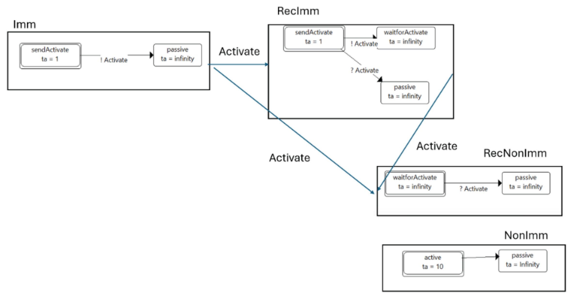
Figure 7.
Example of an Internal Coupling: Component C1 sends unspecified messages on Port PI to Component C2 on Port P2.Example of an Internal Coupling: Component C1 sends unspecified messages on Port PI to Component C2 on Port P2.
Figure 7.
Example of an Internal Coupling: Component C1 sends unspecified messages on Port PI to Component C2 on Port P2.Example of an Internal Coupling: Component C1 sends unspecified messages on Port PI to Component C2 on Port P2.
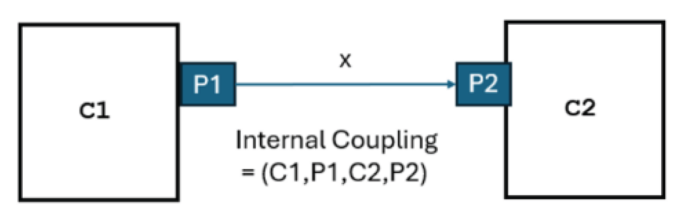
The simulator calls the RouteMessages() algorithm which looks up the table given the source and its output port. The algorithm is briefly described by:
RouteMessage(C1,P1,x) given IC = {(C1,P1,C2,P2)}:
Extract all couplings that have source = C1 and outport = P1
For each such coupling, let the destination = D and inport = IP
return the pairs (D,IP)
Example: In Figure 7, the coupling (CI,P1,C2,P2) has source = C1 and outport = P1, with destination = C2 and inport = P2
Explanation: The simulator calls RouteMessage(C1,P1,x) when C1 is imminent and the call to its output function produces message x; The coordinator places the message x on the inport IP of the destination D by calling D’s external (or confluent) transition function with input x on inport IP.
In the example of Figure 6, components Imm and RecImm are imminent, and place Activate messages on their output ports outActivate. The RouteMessages algorithm looks ups the source/input port pairs for these messages and the coordinator calls either the external transition function or the confluent transition function as described below in step 4).
- (1)
-
The effects of transmitted outputs (now inputs) are computed:
- Since RecImm is imminent and receives an input, it uses its confluent function to compute its next state as waitForActivate (here the confluent function computes the external transition before the internal transition)
- Since RecNonImm is not imminent it uses its external transition function to compute its next state as passive.
- (2)
- Imminent components that are not receivers apply their internal transition functions – here Imm transitions to passive.
- (3)
- Components that are neither imminent nor receive inputs update their time advances to reflect the passage of the elapsed time. Here NonImm updates its time advance to 9. (10. – 1.).
This computed next state is displayed as:

Table 3.
Global State after Transition.
| Component | Sequential State | Time Advance |
|---|---|---|
| Imm (Imminent) | passive | infinity. |
| RecImm (Receives input and is Imminent) | waitForActivate | infinity |
| RecNonImm (Receives input and is not Imminent) | passive | infinity |
| NonImm (NonImminent) | active | 9. |
The next cycle repeats with a minimum time advance of 9 and the clock is updated to 10. Note that NonImm transitions to passive as originally scheduled at this time while the other components remain inactive.
Here we see that the abstract simulator algorithm changes the global state to the correct new configuration with the correct time advance in steps that correspond to those of the proof of Closure under Coupling. When transferred to a network context, the abstract simulator is referred to as the Distributed DEVS Simulation Protocol to reflect that model components may reside on different computing elements and the coupling implemented as routing of messages among them.
Object-Oriented Implementation of DEVS Abstract Simulator
The process of closure under coupling can be viewed as collapsing the entire coupled model into a single behaviorally equivalent DEVS atomic model. The atomic state space is the global state space of the coupled model, i.e.; the Cartesian product of all component model states (plus their elapsed times). The proof proceeds by deriving the form of the basic functions: output, internal, external, and confluent transition, and time advance. For example, the latter compute the global time-advance function (the minimum of the component time advances). The resulting atomic model reproduces exactly the behavior of the original coupled network, but at the cost of a vastly larger state description—yet with zero inter-component message passing at runtime [87].
In this section, we present a new design for object-oriented implementation of the DEVS Abstract Simulator. In contrast to existing designs [2,44,45,46,47,48,49,50,51,52]. The design employs closure under coupling explicitly to simplify the operation of the DEVS simulator, here-after referred to the 2-level DEVS simulator (2DEVSim). It does so by reducing the requirement for coordinators to handle arbitrary hierarchical models so that they only are concerned with models that are instances of the Atomic class as defined in the class structure of Figure 8 a) which illustrates the class structure of DEVSim. In the sketched UML class diagram, the DEVS base class is extended by the Atomic and Coupled subclasses. 2-level DEVS simulator (2DEVSim). It does so by reducing the requirement for coordinators to handle arbitrary hierarchical models so that they only are concerned with models that are instances of the Atomic class as defined in the class structure of Figure 8 a) which illustrates the class structure of DEVSim. In the sketched UML class diagram, the DEVS base class is extended by the Atomic and Coupled subclasses.
An instance of a Coupled class is composed of one or more Atomic instances. Further structuring of these classes reflects the formal definitions of their respective DEVS basic, atomic, and coupled models (not shown in the figure). Classes AtomicSimulator and CoupledCoordinator handle respective instances of Atomic and Coupled. The definitions of these classes follow those of the original implementation except that the CoupledCoordinator can only handle atomic models as opposed to arbitrary coupled models in the original. This simplifies its definition as it does not need to handle the recursion needed for routing messages according to the coupling in the latter. Closure under coupling is the enabler that makes this coordinator design capable of handling hierarchical models. As shown in Figure 8a), this is implemented by introducing the subclass of Atomic called ClosureToAtomic. This class implements the wrapping of a Coupled instance required to make it behave like an Atomic instance to a CoupledCoordinator. Figure 8b) illustrates the inner working of the ClosureToAtomic class. Critical to this wrapper is how the wrapped coupled model interfaces with the AtomicSimulator that will be in charge of executing it. The simulator expects to call the basic functions of the Atomic (internalTransition(),externalTransition(), confluentFunction(), getOutput(), and getTimeAdvance()). This in turn leans on the correct functioning of the internal coordinator (which is an instance of CoupledCoordinator) as it adheres to the simulation cycle derived from the closure under coupling proof. Appendix D shows the inner workings in detail Here we sketch how it works in Table 4:
We note that this construction is based on the concept of wrapping a coupled model to make it appear as an atomic model and does not require flattening the structure, which is an operation that we describe later. The wrapping can be done automatically when the user creates an instance of the CoupledCoordinator and gives it a coupled model to work on.
4. DEVS BUS and Model Transformation
Following the introduction of the DEVS abstract simulator and associated DEVS simulation protocol, we will demonstrate how non-DEVS models can be incorporated within this framework. Figure 9 presents the DEVS bus concept, which enables interoperability with multiple modeling formalisms [52,53,54,55,56,57,58] The ability for DEVS-based simulators to import and export models for integrated simulations, improving compatibility and supporting model sharing and reuse is an area where many DEVS tools still require further development for full interoperability in complex engineering applications [59,60]. To facilitate integration, each formalism must be encapsulated in a DEVS-compliant format through an appropriately defined simulator. These models may then be coupled with others and executed via a standard coordinator. Furthermore, as reviewed above, DEVS possesses the versatility to represent models developed using other prominent formalisms such as DTSS and DESS, thereby making it feasible to unify these within an all-DEVS simulation environment, characterized by the DEVS Bus concept, which supports multiformalism modeling. In the following we discuss transformations of non-modular multi-component models to modular form that enable these formalisms to be adapted for compatibility with basic DEVS. Adaptation occurs by incorporating essential input/output interface elements, namely external transition, and output functions to create so-called DEVS wrappers.
4.1. Transforming Non-Modular Multi-Component DEVS Models into Modular Form
Multi-component systems with non-modular couplings directly access and modify each other’s state variables. This results in a lack of modularity when compared to systems with modular couplings. The following procedure outlines how to convert non-modular coupled systems into a modular structure. This conversion can always be achieved by identifying dependencies between components and restructuring them into input and output interfaces and modular couplings. The process of introducing input/output interfaces is referred to as modularization.
There are two types of non-modular couplings that require different handling. In the first type, component A has write access to a variable v belonging to component B (Figure 10). Modularization transforms this arrangement into a communication from A to B using a modular coupling. Specifically, A is provided with an output port, vout, while B receives an input port, vin, which are connected by a coupling. When A intends to update v in the original transition function, it initiates an output event at vout with the corresponding value in the modular form. This action triggers an input event at vin of B, and B’s external transition function updates its variable v with the received value.
In the second type, component B has read access to a variable u of component A (Figure 10). In the modular form, this scenario requires B to consistently access the current value of u. To address this, B maintains a copy of u’s state information. Whenever A changes the value of u, B must be notified of the modification. This notification occurs through a coupling that connects ports uout on A and uin on B, like the mechanism used in the first case. As a result, B maintains an updated copy of variable u in its own state variable ucopy_(Figure 10). B has read access to a variable u of component A (Figure 10). In the modular form, this scenario requires B to consistently access the current value of u. To address this, B maintains a copy of u’s state information. Whenever A changes the value of u, B must be notified of the modification. This notification occurs through a coupling that connects ports uout on A and uin on B, like the mechanism used in the first case. As a result, B maintains an updated copy of variable u in its own state variable ucopy_(Figure 10).
Non-modular models are often designed as single, rigid structures that are difficult to modify or extend. To convert them to modular form, the model is broken down into smaller, independent components, each representing a distinct part of the system. These components become reusable modules, which can be interconnected using the principles of DEVS closure under coupling. This transformation allows the overall system to be reconstructed as a network of modules, making it easier to manage, maintain, and expand. Additionally, hierarchical organization can be introduced, with modules nested within larger modules, further supporting flexibility and scalability. The modular approach streamlines model design and supports interoperability by enabling uniform treatment and integration of diverse models. Moreover, this approach has the advantage that hierarchical DEVS models can be readily transformed into executable simulation code. Finally, it has the advantage that it supports formalism interoperability. concept, we will show that it allows the integration of modular components formulated in different modeling approaches, supports formalism interoperability. concept, we will show that it allows the integration of modular components formulated in different modeling approaches,
4.2. Non-Modular Non-DEVS Models in Distributed Simulation in Distributed Simulation
The concept of DEVS models coordinated on the DEVS Bus is particularly important in distributed simulation. Non-modular models are models that, unlike their modular counterparts, allow other models to access their internal state. For example, in Figure 11, model B has direct read access to model A during its state transition function. Model B also has direct write access to the state of model C. This type of global state access is common in distributed simulation implementations. Figure 11, model B has direct read access to model A during its state transition function. Model B also has direct write access to the state of model C.
Standardized simulation protocols typically implement their components as non-modular models with a global state sharing mechanism, as shown in Figure 12. This is true for the published SISO standards, High Level Architecture (HLA), and Web Live, Virtual, Constructive (WebLVC) [5,40,61,62,63]. Another characteristic of such distributed simulation standards is to synchronize time via real time, also known as “wall-clock” synchronization. In this paradigm, there is no synchronized global event list, and each model executes events once the real-time clock reaches their scheduled time. This is true for Distributed Interactive Simulation (DIS) IEEE Standard and WebLVC [64]. Another characteristic of such distributed simulation standards is to synchronize time via real time, also known as “wall-clock” synchronization. In this paradigm, there is no synchronized global event list, and each model executes events once the real-time clock reaches their scheduled time. This is true for Distributed Interactive Simulation (DIS) IEEE Standard and WebLVC.
The universality and uniqueness of DEVS representation can be applied to represent non-modular models in DEVS-compliant form. In short, if the non-modular model is a set of functions to produce time-based output streams from time-based input streams, then there is a way to construct an equivalent DEVS model for that non-modular model. DEVS-SF [9,65,66] constructs equivalent DEVS models via DEVS wrappers for existing non-modular protocols using the approach of Section 4.1. Once this is done, they can be executed by a Parallel DEVS Coordinator as if they were Parallel DEVS models, as shown in Figure 13, with a wrapped non-modular WebLVC model. The non-modular system model A publishes its state to the DEVS/WebLVC wrapper. The Parallel DEVS Coordinator then couples model A’s output with the input of Parallel DEVS Model B. [9,65,66] constructs equivalent DEVS models via DEVS wrappers for existing non-modular protocols using the approach of Section 4.1. Once this is done, they can be executed by a Parallel DEVS Coordinator as if they were Parallel DEVS models, as shown in Figure 13, with a wrapped non-modular WebLVC model. The non-modular system model A publishes its state to the DEVS/WebLVC wrapper. The Parallel DEVS Coordinator then couples model A’s output with the input of Parallel DEVS Model B.
The DEVS community has had success in leveraging the universality and uniqueness of DEVS to interoperate with HLA and WebLVC [9,65,66]
Recognizing the DEVS ability to represent DEVS-like systems (Section 4 we can extend the concept of wrapping from an operation on models to a similar operation on simulators of non-modular models.
To elaborate, suppose that we are given a complex coupled model already in executable form such as a federation in HLA. We suppose that, as likely the case in this form, the simulator (e.g.; HLA Runtime Infrastructure) is a DEVS-like system. Then we can treat this simulator as a component in a larger coupled model that we wish to construct.
In practice, this requires that the higher-level simulator can inject inputs, receive outputs, and can query to get the time advance as required by the DEVS abstract simulator.
In summary, the theory provides us with two approaches to convert non-modular coupled models embedded in simulators to modular form for coupling in hierarchical compositions:
- (1)
- Convert the atomic constituents of the coupled model to modular form so that they, as well as the coupled model can be reused.
- (2)
- Treat the existing simulator as a DEVS-like system and wrap it in a form like that of Section 3 in which it appears to be an atomic model to the coordinator of the desired enclosing coupled model.
In this way existing federations of different types can be coordinated within the same coupled model without necessarily refactoring their internal structures. This conclusion carries significant practical implications for distributed simulation. It demonstrates that heterogeneous federations—regardless of their internal architectures—can be orchestrated within a unified coupled model without requiring structural refactoring. This effectively eliminates a key obstacle to broader DEVS adoption, particularly within organizations that maintain substantial legacy simulation assets.
4.3. DEVS Co-Simulation
4.3.1. Functional Mockup Unit (FMU) and Interface (FMI)
The DEVS Bus concept is also essential in co-simulation, a method that connects different simulation models or tools to analyze complex systems. In co-simulation, these models exchange data for a more accurate view of system behavior [11,61,67,68,69,70,71,72,73,74,75,76,77,78]. Co-simulation serves as an essential instrument for the development and management of emerging socio-technical systems that require integrating continuous-time components with event-driven elements. presents significant challenges from both modelling and operational tool perspectives. [67] proposed an approach that exploits the ability of DEVS to integrate the DEV&DESS [79] formalism -which offers a sound framework for describing hybrid models (Section 2). In the following we start from a more fundamental perspective in considering the basic problem of coupling models of different formalisms in a well-defined DEVS composition. The Functional Mockup Interface (FMI) [77,80,81,82,83]. Modelica Association Functional Mockup Interface Standard was developed to standardize model exchange and co-simulation which enables interaction among models developed in different formalisms. FMI defines a C interface that is implemented by an executable called a Functional Mock-up Unit (FMU). Simulation environments use the FMI to create an instance of the FMU to work together with other FMUs or other native models. Ritvik et al. [77,84] developed a framework based on FMI/FMU for exporting and importing modular DEVS models (after non-modular to modular conversion (Section 4.1) if necessary), enabling interoperation of DEVS simulators as formulated in the DEVS Bus concept. Moreover, the framework demonstrates how DEVS can support broader FMI-based co-simulation via standardized integration with tools like MATLAB-Simulink and Open-Modelica [85].
A key aspect of FMI is that each shared model runs independently, synchronizing only at discrete points [82,86]. This aligns well with DEVS coupled model synchronization, defined by closure under coupling. FMI co-simulation’s modular, hierarchical interaction management also matches the DEVS Bus concept, enabling integration with other modeling frameworks for hybrid systems. By combining DEVS with FMI, discrete and continuous-time models can interact seamlessly without redefining existing continuous models [4]. For instance, a DEVS-based navigation system in MS4 Me [88,89] and a vendor created continuous time controller were integrated in the Cadmium DEVS environment [84,90,91] via FMI. As a result, DEVS-based simulators can import and export models for integrated hybrid simulations, improving the opportunity to achieve greater interoperability (Section 8.5).160, 235]. This aligns well with DEVS coupled model synchronization, defined by closure under coupling. FMI co-simulation’s modular, hierarchical interaction management also matches the DEVS Bus concept, enabling integration with other modeling frameworks for hybrid systems. By combining DEVS with FMI, discrete and continuous-time models can interact seamlessly without redefining existing continuous models [87]. For instance, a DEVS-based navigation system in MS4 Me [88,89] and a vendor created continuous time controller were integrated in the Cadmium DEVS environment [84,90,91] via FMI. As a result, DEVS-based simulators can import and export models for integrated hybrid simulations, improving the opportunity to achieve greater interoperability (Section 8.5).
4.3.2. Exporting DEVS Models as DEVS FMUs
Figure 14 illustrates a UML diagram depicting the environment established for exporting a DEVS model as an FMU. FMU4-MS4Me leverages the FMU4J library [81] and its capabilities to package models into FMUs, with extensions developed to facilitate the export of DEVS models created using MS4Me. This functionality is structured through definitions of both generic DEVS operations and model-specific design elements. The DevsFMU and Application model classes, represented in Figure 14, were implemented utilizing the FMU4J and ms4systems [88,89] libraries. The DEVS model package showcased in Figure 14 comprises model code that MS4 Me generates automatically.98] and its capabilities to package models into FMUs, with extensions developed to facilitate the export of DEVS models created using MS4Me.
The DevsFMU class provides core DEVS modelling and simulation (M&S) functionalities; it incorporates Fmi2Helper from FMU4J, which supports FMU export. DevsFMU maintains objects of the model and simulator classes as class variables. Specifically, the model class (CoupledModelImpl) describes the model structure, while the simulator class (SimulationImpl) contains all methods necessary for model simulation—both classes are defined within MS4Me. DevsFMU overrides several Fmi2Helper methods, such as registerVariables, utilized to set and update timeRemaining, which indicates the time until the next event and uses setupExperiment to initiate the simulation. Simulation functions are triggered via the doStep method, which may invoke injectInput from MS4Me to deliver inputs, or otherwise call simulateIterations to execute subsequent simulation steps.
The FMU instantiation and function calls inside the atomic model enable the FMU to connect with the simulator. The doStep function is called by the model’s internal transition function, where the time advance value is used as the next communication point. Advancing time in this way allows the DEVS model within the FMU to function as a single atomic unit, thus using closure under coupling to ensure events follow global simulation time in proper order.
5. Operations on DEVS Model Structure
5.1. Flattening and Its Inverse, Deepening
Flattening in DEVS refers to a structural transformation that eliminates the nested layers of coupled models, resulting in a single level coupled [31,38,39,40]. This process begins with a hierarchical coupled model, traverses its decomposition tree, and reconstructs all inter-component couplings so that each leaf atomic model is connected directly to the top level. The outcome is a flat coupled model whose external interface remains consistent with the original but does not require hierarchy navigation during runtime. Closure under coupling is key to proving the flattened model is equivalent to the original. [31,38,39,40].
Flattening is illustrated in the example of Figure 15a) where on the left of the arrow, a Processor model is coupled to an Experimental Frame, EF. This is a hierarchical coupled model because the frame, EF is itself a coupled model with components, Generator and Transducer. The flattened version is shown on the right of the arrow, where all components are atomic models, Here the couplings are direct from one component to another rather than travelling through hierarchical levels while retaining the identical port-to-port connections. For example, the Generator sends a Job directly to the Processor rather than sending it to its parent, EF, to relay to the Processor. Like the join operation of relational data tables, the operation of merging couplings is illustrated in Figure 16.
[31] provided an algorithm for flattening that represents the topology of connectivity through coupling matrices from each component model, merging them into a global coupling–structure matrix. It then generates the flattened coupling–structure matrix through depth-first search or matrix operations like transitive closure. However, this approach abstracts away the ports involved in the couplings which must be restored in a subsequent phase that is not considered by the authors. Here we provide an efficient algorithm that works directly on the hierarchical model’s composition tree, as illustrated in Figure 15 b). As sketched in Figure 17, the approach is to form a recursion whose basic step is to remove a coupled model from its parent and replace it with its components inserted into its parent’s composition as well as couplings to the parent and its other children that represent the concatenated couplings as in Figure 16. The recursion proceeds by finding a coupled model to eliminate in this manner until no such models are left. The process repeats until all coupled models are eliminated. In a straightforward recursion, it can proceed level by level through the composition tree, restructuring by eliminating coupled models it encounters in a top-down manner. Interestingly, since the tree structure is transformed into the process, the recursion remains focused on the root node while the flattened versions of the successively shallower structure are created underneath it. The computational complexity ranges from constant to exponential in tree depth as it depends on the tree’s growth behavior. However, unless the simulation involves dynamic restructuring, the flattening operation is performed only once while saving numerous hierarchy traversals that would be needed during runtime.14] provided an algorithm for flattening that represents the topology of connectivity through coupling matrices from each component model, merging them into a global coupling–structure matrix. It then generates the flattened coupling–structure matrix through depth-first search or matrix operations like transitive closure.
flatten(CoupledModel) perform a “flattening” operation on a hierarchical coupled model by successively flattening one level of hierarchy: replace all children coupled models with their children so that the parent’s grandchildren become its children and adjust all associated couplings accordingly.
Basic Step: flattenChild(CoupledModel, child) eliminates the coupled model’s child and reconnects its grandchildren to become direct children of the coupled model following the procedure illustrated in Figure 16.
Recursion: flattenChildren(CoupledModel) calls the basic step, flattenChild for each of its non-atomic children. In Java, the operations are performed on a copy of the tree which is then used for the next round. This is to avoid concurrent operation due to the ongoing structural changes.
Termination: The process stops when there are no coupled models with non-atomic model children left. Termination is guaranteed since the tree is finite and the non-atomic nodes (coupled models) are visited exactly once.: The process stops when there are no coupled models with non-atomic model children left. Termination is guaranteed since the tree is finite and the non-atomic nodes (coupled models) are visited exactly once.
5.2. Deepening
Deepening of a hierarchical model is an inverse operation to flattening in which several components are grouped to form a single coupled model with the coupling amended to preserve the model’s behavior. Coupling between components that have become separated by a partition boundary must now be refactored accordingly. This can be visualized in Figure 16 where instead of working from top to bottom, we rewrite the coupling at the bottom to a new pair on the top, where a new port is introduced to mediate the flow from source to the destination. Deepening can be a fundamental process in creating modules where components are grouped into higher level coupled models according to criteria related to design considerations. This is another area for future research as discussed in Section 8.4.
5.3. Implications of Flattening for Design of DEVS Models and Simulators
Flattening in DEVS can have significant execution advantages primarily through reducing inter-component message traffic and removal of intermediary components [39,46,92,93,94,95] but also has downsides that must be considered. Flattening removes intermediate coupled models with the loss of critical information. This renders it potentially less intuitive for human users analyzing system behavior making it difficult to trace or debug the processing flow in the absence of the system’s hierarchical design. It can be more challenging to gain insight during verification and validation (V&V) and to quickly identify errors. This approach is more efficient but provides less information. Similarly, there is less data available for visualizations unless additional logging is implemented, which may slow down the process. A balanced approach may be best: decompose hierarchical models for distribution across nodes, then flatten those assigned to nodes for local execution. We revisit this issue in the discussion of future research (Section 8).
6. DEVS Closure Under Coupling in Relation to Other System Formalism/Frameworks
In this section, we examine DEVS Closure under Coupling in relation to notions in other formal frameworks that exhibit closure properties under various operations. We will see that DEVS closure under coupling is unique in several ways including its origin in mathematical systems theory, its basis for a rigorous method to interpret a coupled model as a basic DEVS model (Section 2), and for definition of an associated abstract simulator (Section 3).
6.1. Wymore’s Mathematical Systems Theory
A. W. Wymore’s work [91,92,93] significantly advanced systems theory, especially in model-based systems engineering, by rigorously formulating the concept of closure under coupling for dynamic systems. His formulation showed that coupled dynamic systems could transform into an equivalent atomic system within the same framework, promoting modularity. Wymore’s precise mathematical foundation supported complex system design and analysis, as detailed in his book, Model-Based Systems Engineering [94]. DEVS as shorthand for specifying a class of Wymore’s systems provides an important computational basis for Wymore’s theory that was heretofore missing. Although related concepts existed in cybernetics, control theory, and automata theory, Wymore’s treatment was one of the earliest and most rigorous. Pioneers like Norbert Wiener [95] and Ross Ashby [96]. dealt extensively with the composition and interconnection of systems. Although their work did not use the same formal language or focus explicitly on “closure under coupling” as later defined by Wymore, they did analyze how systems interacted and how their collective behavior could be understood as part of a unified whole.
6.2. Automata Theory and Formal Languages
In automata theory [97], the class of regular languages is closed under operations such as union, concatenation, and Kleene star. Each of these operations corresponds to a coupling of finite automata that individually accepts a language, and proof of closure is obtained by showing that the resulting composite is still a finite automaton. In that sense, the proof of closure for DEVS is a generalization of the related automata theory concept. In fact, it can be shown that, interpreted as DEVS models, the set of finite state systems is closed under coupling [17].
6.3. Process Algebras (e.g.; CSP, CCS, π-calculus [98,99]
Process algebras offer methods for describing systems through the parallel and sequential composition of processes. By combining individual processes, a new process is created that conforms to the algebra’s semantics. This combination often remains implicit, with the resulting system requiring additional semantic elements like synchronization or communication channels. DEVS extends this concept by allowing the coupled system to be explicitly reconstituted as a basic DEVS model. This explicit conversion provides a formal guarantee that enhances DEVS’s suitability for hierarchical modeling, enabling simulation engines or analysis tools to handle a coupled system as a single unit in appropriate contexts.
Petri Nets and Other Graph-based Formalisms [100,101,102,103,104]
When connecting Petri nets, the resulting network is often still a Petri net with the same properties (places, transitions, tokens). However, while compositional methods exist, the transformation from a network of coupled nets into a “single net” is not always as straightforward or canonical as in DEVS. The DEVS closure property guarantees that every coupled model can be transformed into an equivalent basic DEVS model by a systematic procedure. This kind of formal “flattening” of the structure is not as universally available or as well-defined in all other modeling frameworks. Moreover, the inclusion of elapsed time as a fundamental state variable in DEVS (Section 2.1) is salient as the missing concept in Petri nets limited compositionality.
Control Theory and Linear Systems [151]
In control theory, the interconnection of linear systems results in another linear system. This closure property under interconnection is crucial for analyzing complex control loops. As with finite state systems, linear systems constitute a class of Wymore systems and can be specified as special cases of DESS and DTSS (Section 2.2).
Although both share this idea, DEVS addresses discrete events rather than continuous dynamics. The DEVS framework’s advantage is its ability to represent a highly interconnected network of discrete-event systems, which may operate with asynchronous timing and event-driven transitions, as a single, well-defined DEVS model.
In summary, many formal frameworks exhibit closure properties under various definitions and operations to ensure that the system’s integrity is maintained. DEVS closure under coupling stands out because it not only tells us that the composition remains within a “system” class but also provides a rigorous method to reconstruct the coupled system as a DEVS atomic model and an associated abstract simulator. This unique feature reinforces the utility of DEVS in modular and hierarchical modeling, making it easier to build, analyze, and simulate complex discrete-event systems.
7. Discussion and Summary
7.1. Hierarchical Modular Construction and Multi-Resolution Modeling
Sisti [116] was early recognizer of the need for moving away from desire for a single comprehensive model. He concluded that modeling of largescale and complex software systems requires multi-resolution modeling, i.e.; following a convention of multiple levels of representation, such that the entities are modeled at varying levels of detail, ranging from the top-level representation of the “essence” of the entity, to the lowest level, which would model the entity in great detail.
Multi-resolution modeling [10,44,47,51,61,78,112,113,114,115,116,117,118,119,120,121,122,123,124,125,126].
must bring to bear a variety of technical, theoretical and practical aspects: including modularity, software reuse, object-oriented design, a hierarchy of models in a component library, and a model management system for manipulating such repositories. Anticipating the later MOSA directive (Section 8.1), Sisti concluded that an approach to modularization must be developed in which modules interact through defined interfaces, protecting implementation details via data abstraction and encapsulation. He saw the benefits of modularity as:
- Easier development of correct models due to smaller, manageable modules.
- Streamlined design and coding, as modelers focus on core functionality.
- Support for parallel development by multiple collaborators with controlled interactions.
- Simplified maintenance and reconfiguration as system requirements evolve.
- Use of component hierarchies for flexible system modeling at different levels of detail.
- Enhanced software reuse, paving the way toward standardized models and libraries.
7.2. Application of DEVS Concepts to MOSA
United States Department of Defense (DoD) instructions such as DoDI 5000.02 [18,139] encourage iterative development, builds, integration, testing, production, certification, and deployment of software systems to the operational environment as mandated by requirements such as Title 10 USC 2446a, The Modular Open Systems Approach (MOSA) is a technical and business strategy that integrates engineering with procurement and lifecycle management, helping ensure systems are agile, cost-efficient, and compliant with DoD acquisition reforms. While “Modular Open System Architecture” often refers to system structure, it refers to a comprehensive strategy for acquiring and upgrading systems through modularity and open interfaces. transforming the traditional “monolithic” approach, the goal is to make components interoperable, reconfigurable, and upgradeable throughout a system’s lifecycle, encourage iterative development, builds, integration, testing, production, certification, and deployment of software systems to the operational environment as mandated by requirements such as Title 10 USC 2446a, The Modular Open Systems Approach (MOSA) is a technical and business strategy that integrates engineering with procurement and lifecycle management, helping ensure systems are agile, cost-efficient, and compliant with DoD acquisition reforms. While “Modular Open System Architecture” often refers to system structure, it refers to a comprehensive strategy for acquiring and upgrading systems through modularity and open interfaces. transforming the traditional “monolithic” approach, the goal is to make components interoperable, reconfigurable, and upgradeable throughout a system’s lifecycle,
As illustrated in Figure 18, MOSA is guided by a planning framework that specifies the following stages:
Plan: Set objectives that match technical and business needs.
Modularize: Break system functions into self-contained modules with clear interfaces.
Identify interfaces: Specify standardized interfaces based on open standards for smooth module integration.
Define interface specifications: Detail module interactions with standard protocols and formats for compatibility.
Standardize interfaces: Support modular design and resilience to future technology changes.
DEVS theory provides foundational mechanisms—such as closure under coupling, universality, and uniqueness—that are applicable to the Modular Open Systems Approach (MOSA) in simulation contexts. As illustrated in Table 5, DEVS principles also apply more generally to support the MOSA framework for building and upgrading software-intensive systems through modularity and open interfaces. Closure under coupling in DEVS ensures that interconnected models, whether atomic or coupled, can be composed into a single unified model without leaving the formal DEVS framework. This modularity enables the construction of complex, hierarchical systems from simpler, reusable components, streamlining model management and supporting scalability. The transformation from non-modular to modular form and hierarchical structures makes models easier to maintain, integrate, and expand, which is essential for MOSA’s emphasis on interoperability and reuse. DEVS universality and the uniqueness of representation guarantee that any system characterized by discrete event interfaces and behaviors can be accurately modeled and executed within the DEVS framework. This provides a common formal basis for representing diverse systems, which is crucial for MOSA implementations that require consistent, reliable integration across heterogeneous platforms.
Flattening and hierarchical organization in DEVS allow nested models to be represented and executed as atomic entities, preserving behavioral equivalence and facilitating efficient simulation execution. This supports MOSA objectives by enabling uniform treatment and integration of models, regardless of complexity or origin.
In summary, applying DEVS concepts to MOSA enables simulation architectures to uniformly and efficiently integrate, execute, and manage diverse systems, thereby enhancing interoperability, scalability, and maintainability – not only across military simulation initiatives but to software system development more generally.
8. Directions for Research
8.1. MOSA Related Research
A major theme for future research is the development of a MOSA-Compliant DEVS Reference Architecture. This would define a reference architecture that explicitly aligns DEVS modularity with MOSA principles, including interface contracts, plug-and-play model integration, and lifecycle management.
For example, it might include the following:
- Propose a DEVS profile or annex for MOSA-related standards, specifying minimal compliance requirements for closure, universality, and uniqueness.
- DEVS profiles for MOSA interface standardization: Propose a DEVS “profile” that defines minimal, machine-readable interface specs (ports, timing, QoS) and verification steps to satisfy MOSA’s open interface requirements; include acquisition-relevant artifacts.
- Cross-Domain Model Federation: Demonstrate DEVS-based integration of models from related domains into a unified MOSA-aligned simulation environment.
- Lifecycle modularity metrics for DoD programs: Empirically measure integration time, defect rates, and upgrade costs when programs adopt DEVS-based modular simulation architectures under MOSA; compare against legacy bespoke integrations.
8.2. Formal Theory Extensions
8.2.1. Extend Closure Under Coupling Theory and Apply to Important Classes of Models
Research can be done to extend DEVS closure to hybrid co-simulations that mix discrete event, discrete time, and continuous subsystems. Appendix E reviews literature on closure under coupling in DEVS-related system specifications, broadening understanding of its modeling and simulation implications. Like the squares example (Section 2.2), failure of coupling closure suggests a need for more flexible definitions or newly considered dimensions. In this paper, closure is highlighted as supporting hierarchical modular model construction, ensuring well-definition, composability, and reuse. However, research is also needed to elucidate drawbacks of such redefinition in representative cases.
8.2.2. Exploit Uniqueness of DEVS Representation for Basic Building Blocks
Uniqueness of DEVS in representation of DEVS-like systems is akin to the realization theory as mentioned above and generalizes to the hierarchy of systems specifications and morphisms [50,114,120,131,140,141,142,143,144,145,146,147,148] which can offer the basis for definition of building blocks and architectural patterns that can be replicated and reused in system development. Research can be done to identify elements of this kind and establish their status as minimal realizations of their defined behaviors. Besides having computational advantages, such minimal designs must ipso facto underlie any implementation of the said behaviors. Future research can be focused on using and extending the methodology for further exploring potentially useful DEVS building blocks and architectural patterns for Internet of things Cyberphysical systems [37,149,150,151,152,153].
8.3. Support for Model and Simulation-Based System Engineering
DEVS support for collaborative simulation can enable domain experts and modelers to work together to build, integrate, and simulate models, often facilitated by web-based environments, middleware, or shared libraries of reusable models [6,16,19,20,21,22,23]. In this context, research is needed to address the challenge of integrating models developed in different tools by providing a common framework for collaboration and model exchange, leading to more realistic and comprehensive simulations.
DEVS can be conjoined with Wymore mathematical systems design theory (Section 6) to provide a more scientific basis for systems engineering [14,27,97,154]. Here, DEVS can serve as a core component of Model-Based Systems Engineering (MBSE) by providing a theoretically grounded way to connect a system’s blueprint (architecture models) with its performance and behavior. Research in this direction is needed to address limitations in current MBSE system specification connectivity to simulation and ability to seamlessly integrate different component MBSE specifications into a unified whole for multi-component systems. Further, in the context of MOSA and its simulation incarnation, there is an opportunity to combine Wymore’s theory, DEVS theory, and MBSE concepts to more formally represent executable system models. In this case, DEVS hierarchical coupled models can faithfully represent the System of Systems structure of the to-be-built real system. Further research can explore how the DEVS model provides cost and performance feedback for buildable design alternatives in an iterative design process when executed in experimental frames defined by Wymore’s levels of systems design. Indeed, research is needed to explore in depth, how the application of DEVS concepts within MBSE and systems theory can enable formal analysis of complex MOSA designs within DoD. In particular, continuous simulation-based testing and verification, achieved through the creation of executable MBSE Digital Twins grounded in the DEVS formalism, enables persistent simulation across the entire system life cycle—from conceptual design to operational deployment. This approach supports early detection and correction of design errors, reduces development risks, and facilitates a seamless transition from design models to real-world implementation [155,156]. By leveraging DEVS-based digital twins, system engineers can ensure model continuity, maintain semantic fidelity, and provide a rigorous foundation for verification and validation throughout evolving system configurations.. Further, in the context of MOSA and its simulation incarnation, there is an opportunity to combine Wymore’s theory, DEVS theory, and MBSE concepts to more formally represent executable system models. In this case, DEVS hierarchical coupled models can faithfully represent the System of Systems structure of the to-be-built real system. Further research can explore how the DEVS model provides cost and performance feedback for buildable design alternatives in an iterative design process when executed in experimental frames defined by Wymore’s levels of systems design. Indeed, research is needed to explore in depth, how the application of DEVS concepts within MBSE and systems theory can enable formal analysis of complex MOSA designs within DoD.
More research can be done to generalize the concept of co-simulation (Section 4.3). One direction is to step back to examine the general concept without reference to FMIs. A DEVS simulator can execute in synchrony with an HLA federation where each can share global state variable data with the other. Problems not yet mentioned are the quantized state representation of continuous trajectories [157,158,159,160,161,162,163,164,165,166,167,168] and the location of state events [169] in coupling of hybrid component. Camus [61] presents a co-simulation framework employing the universality of DEV&DESS and its formally defined approach to locating state events in differential equation components attaining capability to modify event-detection functions and to handle discrete internal transitions. The Heterogeneous Flow System Specification [24.29] provides a more general approach that is not fully integrated within DEVS limiting its effectiveness. Research is needed to identify modes of global state sharing that are effective and efficient where non-modular models possibly expressed in different formalisms are involved as in hybrid systems.
Research can be done in ways to implement DEVS simulations using data distribution middleware by mapping DEVS message semantics to Open Management Group data distribution quality of service profiles and event streaming systems such as Kafka, and test for causal delivery, latency limits, and backpressure handling.
8.4. Flattening and Deepening
Research can be done to help to deal with the issue of retaining the benefits of flattening while mitigating against the loss of information that it entails. As summarized in Table 6, flattening of hierarchical structure has consequences in multiple aspects that rely on such structural knowledge. Typically, dynamic structure change involves components and couplings at their locations in the original hierarchical structure [1,94,143,170,171,172,173,174,175]. In the absence of such information, it may be complex to implement dynamically changing models or those requiring frequent updates. Similarly, modular components are generally easier to reuse across different models. Similarly, partitioning flattened models for parallel [2,9,45,51,65,112,176,177,178,179,180,181,182,183] or distributed simulation [2,9,35,63,65,85,112,176,181,184] 185,186,187,188,189 may be more complex due to the reduced modular boundaries, affecting load balancing. In the absence of hierarchy, supplementary metadata or annotations are needed to convey the original design intent. Concerning scalability [31,38,39,40] flattening typically results in a combinatorially greater number of direct couplings, possibly increasing memory consumption and computational requirements during initialization. Research is needed to identify and provide tools for recovering the initial modular structure such as maintenance of comprehensive throughout the transformation process [1,94,143,170,171,172,173,174,175]. In the absence of such information, it may be complex to implement dynamically changing models or those requiring frequent updates. Similarly, modular components are generally easier to reuse across different models.
As discussed above deepening as the inverse of flattening trades visibility for abstraction is powerful for modularity, reuse, and scalability, but it requires discipline in documentation and validation to avoid hidden complexity. As with flattening, research can be done on clarifying and tool development as illustrated in Table 7 that captures the benefits and drawbacks of deepening in hierarchical DEVS modeling:
Of course, as two sides of the same coin, research may examine both deepening and flattening operations together to address the identified issues in a unified way.
8.5. DEVS Standard for Interoperable Simulation Modules
Continued research is needed to develop a robust DEVS standard for interoperable simulation modules. This needs to pursue a multi-pronged research agenda that bridges formalism, middleware, tooling, and community adoption. As suggested before, the ability to wrap legacy simulation engines in DEVS-compliant shells is critical to enable MOSA-aligned reuse without full rewrites.
A summary of the main challenges in developing a DEVS standard for interoperable simulation modules appears in Table 8.
This agenda can be carried out along the following lines:
8.5.1. Continue Research in Tool Development and Language Interoperability
To facilitate DEVS module integration across various programming languages such as Python, Java, and C++, it is essential to develop adapters that bridge these environments. Establishing neutral serialization formats like JSON and XML will further support cross-platform DEVS model exchange. Additionally, exploring the development of editors capable of generating standard-compliant DEVS code and metadata can enhance usability. Defining machine-checkable interface contracts for DEVS components—including specifications for types, timing guarantees, and exception semantics—will enable the auto-generation of adapters, ensuring seamless interaction among heterogeneous simulation units.
8.5.2. Continue Developing Validation, Benchmarking, and Use Case
To advance the standardization and practical adoption of DEVS-based simulation modules, it is crucial to develop benchmark models explicitly designed for interoperability testing across widely used tools such as CD++, DEVSJava, and PyDEVS. By applying the emerging DEVS standard to diverse application domains—including satellite networks, cyber-physical systems, and command-and-control simulations—researchers can rigorously evaluate the framework’s versatility and effectiveness. Furthermore, specifying robust metrics for model reuse, execution accuracy, and integration effort will provide quantifiable means to assess the value and maturity of DEVS implementations. This approach not only facilitates objective comparison among different tools and domains but also drives improvements in usability, reliability, and the seamless integration of heterogeneous DEVS modules.
8.5.3. Continue Integration of DEVS into M&S Community and Standards
To achieve broader compatibility and foster robust interoperability in simulation module development, it is essential to continue to align the DEVS framework with widely adopted standards such as HLA (High Level Architecture) [5,37,57,58,59] and FMI (Functional Mock-up Interface) [73,76,77,78,79,80]. Maintaining an open-source, modular DEVS engine as a reference implementation will serve as a foundational tool for the community, promoting transparent validation and extensibility. Furthermore, establishing a consortium dedicated to overseeing DEVS standardization, regular updates, and certification processes will help unify fragmented research efforts and ensure the consistent evolution and adoption of interoperable DEVS-based simulation modules.
8.6. Towards a Framework for Modeling and Simulation Complexity
Defining and applying measures of complexity to processes, procedures, and algorithms fundamental to M&S activities is an area of research critical to further development. Complexity can be addressed at three levels: 1) Execution Complexity (e.g.;[46] with focus on the baseline efficiency of the simulation engine and metrics for Event scheduling complexity (priority queues, calendar queues), Transition function evaluation cost and Message passing and synchronization overhead. 2) Descriptive Complexity (Model-Centric) to capture the cognitive and informational load of the model itself, independent of execution e.g.; [90]) with focus on information richness and representational burden of the model and metrics such as Kolmogorov complexity (minimum description length of the model). Model scope (breadth of phenomena represented), Resolution (granularity of state variables, time granularity), Output: Quantitative measure of model detail and abstraction cost.; 3) Structural Complexity (Architecture-Centric) to explain how design choices in model organization affect both algorithmic and descriptive complexity, e.g.; [39,60,190] with focus on how model architecture affects computational performance and metrics such as coupling density (number of interconnections between components). Synchronization overhead and trades between modularity (ease of reuse, clarity) and performance (execution cost).
9. Conclusions
DEVS (Discrete Event System Specification) theory establishes fundamental mechanisms—such as closure under coupling, universality, and uniqueness—that are vital for constructing interoperable simulation architectures. The closure under coupling principle enables the composition of interconnected models, whether atomic or coupled, into a unified model that remains consistent with the formal DEVS framework. This approach enhances modularity, supporting the development of complex, hierarchical systems from simpler, reusable components, thereby improving model management, scalability, and facilitating both interoperability and reuse.
Additionally, transitioning models from non-modular to modular and hierarchical forms enhances maintainability, integration, and extensibility. The flattening process ensures that nested, hierarchical models may be represented and executed as atomic entities, preserving behavioral equivalence while promoting execution efficiency. This capability allows DEVS-based simulation architectures to standardize the handling of diverse models, regardless of complexity or origin, thus simplifying simulator design and advancing the integration of heterogeneous systems for broader simulation interoperability.
The principles of DEVS universality and uniqueness of representation ensure that any system with discrete event interfaces and behaviors can be faithfully modeled and implemented within the DEVS framework. This systems-theory based foundation is essential for achieving reliable and consistent integration across heterogeneous platforms, providing the necessary expressive power to accurately capture the internal dynamics expressed in different systems formalisms. Collectively, these DEVS mechanisms—closure under coupling, modularity, and hierarchical modeling—enable the development of efficient simulation engines that treat DEVS models uniformly. Universality and unique representation further strengthen the framework’s efficacy in development of multi-resolution families of models, execution, and interoperability. The mechanisms offered by DEVS theory also enable robust simulation interoperability for diverse and complex systems. Moreover, applying DEVS concepts to MOSA enables interoperability, scalability, and maintainability of software system architectures more generally. While the DEVS principles provide the basis for these advances, as has been pointed out, much research remains to be done to operationalize them into concepts, tools, and standards that are widely adopted.
Author Contributions
Conceptualization, B.Z. and R.K.; G.W.; methodology, B.Z. and R.K.; G.W.; software, B.Z. and R.K.; G.W.; validation, B.Z. and R.K.; G.W.; formal analysis, B.Z. , investigation, B.Z.; resources, R.K.;G.W.; data curation, R.K.;G.W.; writing—original draft preparation, B.Z. writing—review and editing, B.Z. and R.K.;G.W.; visualization, B.Z..; supervision, B.Z.; project administration, B.Z. .: Conceptualization, B.Z. and R.K.; G.W.; methodology, B.Z. and R.K.; G.W.; software, B.Z. and R.K.; G.W.; validation, B.Z. and R.K.; G.W.; formal analysis, B.Z. , investigation, B.Z.; resources, R.K.;G.W.; data curation, R.K.;G.W.; writing—original draft preparation, B.Z. writing—review and editing, B.Z. and R.K.;G.W.; visualization, B.Z..; supervision, B.Z.; project administration, B.Z. .
Funding
Gabriel Wainer received funding from NSERC.
Data Availability Statement
No data sets were used in this research.
Conflicts of Interest
B.Z. is an employee at a company that develops software mentioned in the paper. R.K. performs development and consulting using the DEVS-Streaming Framework mentioned in this paper. G.W. declares no conflict of interest.
Abbreviations
The following abbreviations are used in this manuscript:
DESS Differential Equation System Specification
DEV&DESS DEVS and DESS
DEVS Discrete Event System Specification
DTSS Discrete Time System Specification
FMI Functional Mock-up Interface
M&S Modeling and Simulation
MOSA Modular Open System Approach
SES System Entity Structure
Appendix A
Closure of Rectangles Under Attachment
The concept of closure under an operation is a mainstay in group theory and its generalization and abstractions are expressed in category theory [182]. We offer an intuitive formulation to help understand the essential features in the DEVS context. Figure 1 shows two shapes (rectangles or squares) joined along a congruent side. When attaching two rectangles along this side, the resulting shape is always a rectangle. However, attaching two squares does not result in a square.
In Figure 1, consider R1 with sides L and W1, and R2 with sides L and W2. Aligning them to share the side length L ensures all edges are parallel or perpendicular. The final shape has width L and length equal to W1+W2 the sum of the unattached sides. Since both R1 and R2 have four right angles, the overall figure retains these angles without protrusions, forming a rectangle.
Attaching two squares along an entire side of length L forces them to be geometrically congruent and creates a rectangle with sides of length 2L and L, respectively, i.e.; not a square. Therefore, rectangles retain their type under attachment of congruent sides, while the subclass of squares does not. It is interesting to consider the case where two rectangles happen to form a square under attachment – this does not contradict the closure property because square are rectangles and closure still holds.
Appendix B
Sketch of Proof of Closure Under Coupling
To show that a coupled model composed of Parallel DEVS atomic models can be represented as a single equivalent Parallel DEVS atomic model, the steps are sketched ss follows: coupled model composed of Parallel DEVS atomic models can be represented as a single equivalent Parallel DEVS atomic model, the steps are sketched ss follows:
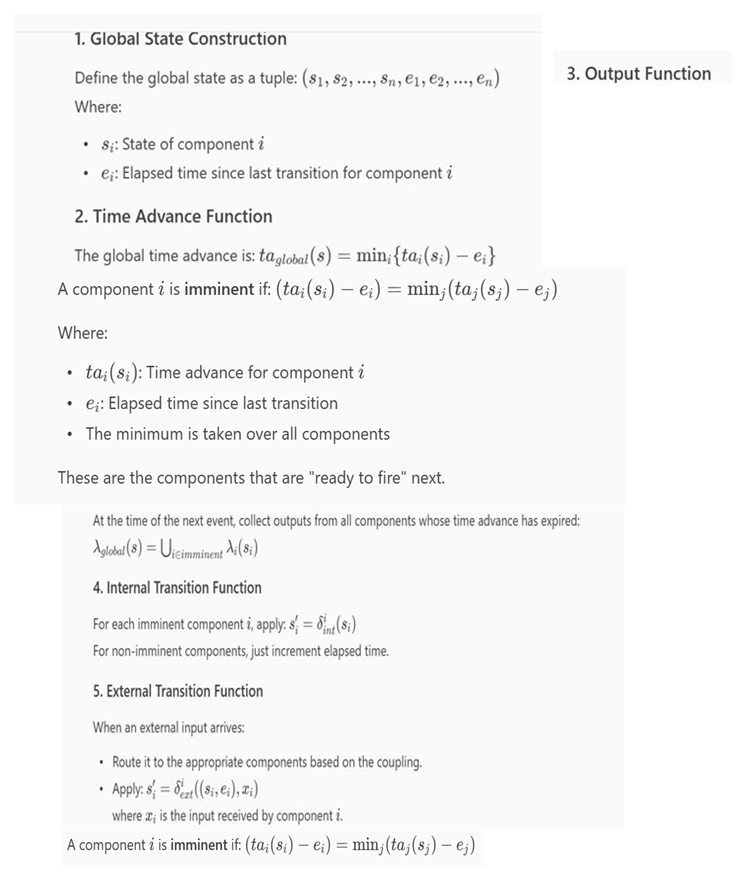
In Parallel DEVS, a component is called imminent if it is scheduled to make an internal transition at the current simulation time.
When imminent components generate outputs, those outputs are.routed to other components based on the coupling specification of the coupled model.
Coupling Types:
- Internal Coupling: Output of one component becomes input to another component.: Output of one component becomes input to another component.
- External Output Coupling: Output of a component becomes output of the entire coupled model.: Output of a component becomes output of the entire coupled model.
- External Input Coupling: Input to the coupled model is routed to one or more components.: Input to the coupled model is routed to one or more components.
Output Handling Process:
- Each imminent component produces an output via its output function produces an output via its output function.
-
The coupling map determines:
- o
- Which components receive these outputs as inputs.
- o
- Whether any outputs are sent to the environment.
- The receiving components then process these inputs via their external transition functions at the same simulation time.
If a component is both:
- Imminent (scheduled for internal transition), and
- Receives input from another component at the same time, then it uses the confluent transition function to resolve the simultaneous internal and external events .
The Resultant (result of construction) has a well-defined state space, transition functions, and time advance as required by an atomic DEVS. Moreover, it behaves identically to the coupled model from an external observer’s perspective. More to the point, it defines what a simulator must do to generate the behavior of the coupled model. Indeed, this process is what guides the definition of the abstract DEVS simulator.
Appendix C
Overview of the DEVS Simulation Protocol
The protocol is typically implemented using hierarchical message-passing architecture involving three main roles:
1. Simulator
- Assigned to atomic model
-
Responsible for:
- o
- Managing the model’s state and time
- o
- Executing internal, external, and confluent transitions
- o
- Generating outputs
2. Coordinator
- Assigned to each lcoupled model
-
Responsible for:
- o
- Coordinating simulators and/or other coordinators
- o
- Routing messages between components
- o
- Managing time synchronization
3. Root Coordinator
- Top-level controller
- Starts and manages the global simulation loop
Message Types in the Protocol
| Message | Purpose |
| init(t) | Initialize model at time t |
| star(t) | Trigger internal transition at time t |
| x(t, value) | Deliver external input at time t |
| y(t, value) | Output message from a model |
| done(t, ta) | Report completion of transition and next scheduled time |
Simulation Cycle
-
Initialization::
- o
- init(t0) messages are sent to all components.
- o
- Each simulator replies with done(t0, ta) indicating its next event time.
-
Time Advance::
- o
- The coordinator determines the minimum next event time across all components.
-
Internal Transition::
- o
- For imminent components, star(t) is sent.
- o
- They compute output (λ) and apply internal transition (δ_int).
- o
- Output is sent via y(t, value) and routed to other components though the internal coupling to receiver components as x(t, value)
| Deliver external input at time t |
When a component receives input at time t, it processes it
- 4.
-
External Transition::
- o
- using δ_ext ,if it is not also an imminent component
- 5.
-
Confluent Transition::
- o
- Using, δ_con, if it is also imminent.
- 6.
-
Completion::
- o
- Each component sends done(t, ta) to indicate its next scheduled event.
- 7.
-
Repeat::
- o
- The root coordinator advances time and repeats the cycle.
Appendix D
Code Sketch of Object-Oriented Implementation of DEVS Simulator
Critical to wrapping of a coupled model is how the wrapped model interfaces with the AtomicSimulator that will be in charge of executing it. The simulator expects to call the basic functions of the model (internalTransition(),externalTransition(), confluent Function(), get Output(), and getTimeAdvance(). This in turn leans on the correct functioning of the internal coordinator as it adheres to the simulation cycle derived from the closure under coupling proof – but only on what appear to be atomic models. Following are the methods in the ClosureToAtomic subclass of Atomic that are responsible for transitioning the model’s state, processing external inputs, producing output, and determining the time until the next event.
An instance of this class wraps a coupled model and its coordinator as instance variables and delegates calls to their simulation methods as described in Java: wrapped model interfaces with the AtomicSimulator that will be in charge of executing it. The simulator expects to call the basic functions of the model (internalTransition(),externalTransition(), confluent Function(), get Output(), and getTimeAdvance().
Following are the methods in the ClosureToAtomic subclass of Atomic that are responsible for transitioning the model’s state, processing external inputs, producing output, and determining the time until the next event. An instance of this class wraps a coupled model and its coordinator as instance variables and delegates calls to their simulation methods as described in Java:
Internal Transition Function is an operation that performs an internal transition when a scheduled internal event occurs.
public void internalTransition() {
// Retrieve the time of the next scheduled event.
double t = internalCoord.getNextEventTime();
// Execute the event that occurs at time ‘t’.
internalCoord.executeNextEvent(t);
}
External Transition function is an operation that processes an external transition given.
public void externalTransition(double timeElapsed, MessageBag input) with arguments, timeElapsed the time elapsed since the last event and input, a MessageBag containing the external input messages.
// Fetch the time at which the last internal event occurred.
double t = internalCoord.getLastEventTime();
// Process the new external input at the updated current time.
internalCoord.processInput(t + timeElapsed, input);
}
Confluent Transition function is an operation handling co-scheduled internal and external transition: here shown with the default in which the internal transition occurs first.
public void confluentTransition(MessageBag input) {
internalTransition();
externalTransition(0, input);
}
Output function is a query that retrieves the output messages generated by the model.
public MessageBag getOutput() {
// Return the computed output from the coordinator.
return internalCoord.computeOutput();
}
Time advance function computes the time advance until the next scheduled state change for this component.
public Double getTimeAdvance() {
// Calculate and return the time until the next event as the difference
// between the next event and the last event t time
return internalCoord.getNextEventTime() - internalCoord.getLastEventTime();
}
Note that these methods lean on the correct functioning of the internal coordinator as it adheres to the simulation cycle derived from the closure under coupling proof – but only on what appear to it as atomic models.
Appendix E
Closure Under Coupling for Other DEVS-Related System Specifications
Closure under coupling justifies hierarchical construction and flattening from coupled to atomic models [49] as well as assuring that the class under consideration is well-defined, enabling checking for the correct functioning of coupled models].
Reference [17] established closure under coupling is established for various system specification classes. The case of DEV&DESS (brought up interesting complexities. In showing that DEV&DESS is closed under coupling, Praehofer [22,50] considered a) the pairs of input-output interfaces between the different types of included systems, b) the means to specify types of components with intermingled discrete and continuous expressions, and c) an abstract simulator to establish that the new formalism could be implemented in computational form.
Besides closure under coupling, two types of questions arise for such formalisms: 1) are they subsets of DEVS, behaviorally equivalent to DEVS but more expressive or convenient, or bring new functionality to DEVS, and 2) have simulators been provided for them to enable verification and implementation? [40] provides examples of DEVS-based formalisms where these questions arise. Overall, such proofs can be exercises in reducing the additional functionality to that available in DEVS itself by expanding the state set sufficiently to support their explicit operation in DEVS. Besides supporting hierarchical construction such exercises can push the designer toward well-definition of the formalism itself in an iterative development process. A variety of examples from DEVS literature are also discussed that either consider closure under coupling explicitly (RoutedDEVS [137] and Multi-Level DEVS [117]) or do not do so but could benefit from doing so (MinMax-DEVS) [7,8]. The former offer instances to examine the significance of the concept and its proof in context as well as to generalize on these issues. The latter offers an opportunity to address what might be missing in the formalism as presented and what benefits might be derived from considering the closure under coupling property for the introduced formalism. Absence of closure is also informative as it begs for characterizing the smallest closed class that includes the given class.
As illustrated by the above cases of finite state and linear systems, closure under coupling is property that is informative for classes of systems that are defined to address requirements [40]. As with the example of squares under attachment, failure of coupling closure can point to the need for greater flexibility in the definition or other dimensions not recognized earlier. As with finite systems, holding of the property may provide concomitant benefits but may come at the expense of limitations in expressiveness that prevent desired application. From the perspective of this paper, such closure is an important property that supports hierarchical modular model construction and the associated advantages of well-definition, composability, and reuse.
References
- Barros, FJ. 2018 Modular representation of asynchronous geometric integrators with support for dynamic topology. SIMULATION 2018, 94, 259–274. [Google Scholar] [CrossRef]
- Chow, A. C. “Parallel DEVS: a parallel, hierarchical, modular modeling formalism and its distributed simulator.” *Trans. Soc. Comput. Simul. Int.*, vol. 13, pp. 55–67, 1996.
- Hwang, M. H.; Zeigler, B. P. “A modular verification framework using finite and deterministic DEVS.” In Proceedings of 2006 DEVS Symposium. 2006; 57–65. [Google Scholar]
- Shiginah, F. A.; Zeigler, B. P. “Transforming DEVS to non-modular form for faster cellular space simulation.” In *Proceedings of 2006 DEVS Symposium*, 2006, pp. 86–91.
- Zeigler, B. H. S. Sarjoughian. 1999. “Support for hierarchical modular component based model construction in DEVS/HLA.” Simulation Interoperability Workshop, March 14 19, Orlando, FL.
- Breunese, A. P. J.; Top, J. L.; Broenink, J. F.; Akkermans, J. M. 1998. “Libraries of Reusable Models: Theory and Application.” Simulation. Vol. 71, (July): pp. 7 22.
- Hamri, E.A.; Giambiasi, N.; Frydman, C. ; 2006. Min–Max-DEVS modeling and simulation. Simulation Modelling Practice and Theory 14, 909–929.
- Hamri, M.E.-A.; Giambiasi, N.; Frydman, C. ; 2006. Min–Max-DEVS modeling and simulation. Simulation Modelling Practice 34 and Theory 14 (7), 909–929.
- Kewley, R.; et al. 2016 DEVS Distributed Modeling Framework - A parallel DEVS implementation via microservices,2016 Symposium on Theory of Modeling and Simulation (TMS-DEVS). 3-6 April 2016.
- Muzy, A.; Touraille, L.; Vangheluwe, H.; Michel, O.; Kaba Traoré, M.; Hill, D. ; 2010. Activity regions for the specification of discrete event systems. In: Spring Simulation Multi-Conference Symposium on Theory of Modeling and Simulation (DEVS), pp. 176–182.
- Risco-Martín JL, de la Cruz JM, Mittal S, et al. EUDEVS: executable UML with DEVS theory of modeling and simulation. SIMULATION 2009, 85, 750–777. [CrossRef]
- Seo, C.; Zeigler, B.; Wainer, G.; Mosterman, P. (2012) Simulation model standardization through web services Proceedings of the 2012 Symposium on Theory of Modeling and Simulation - DEVS Integrative M&S Symposium10.5555/2346616.2346662(1-8)Online publication date: 26-Mar-2012.
- Traore, M.K. A. Muzy. 2006. “Capturing the Dual Relationship Between Simulation Models and Their Context.” Simulation Modeling Practice and Theory, Vol. 14, No.2, (February): 126 142.
- Wach, P.; et al. (2022). “Pairing Bayesian Methods and Systems Theory to Enable Test and Evaluation of Learning-Based Systems.” INSIGHT 25(4): 65-70.
- Zeigler, BP. Theory of modelling and simulation. New York: John Wiley & Sons, 1976.
- Zeigler, B. P. (2022) ‘A methodology to characterize simulation models for discovery and composition: a system theory-based approach to model curation for integration and reuse’, Int. J. Simulation and Process Modelling, Vol. 19, Nos. 1/2, pp.3–13.
- Zeigler, B. P.; Muzy, A.; Kofman, E.; Theory of Modeling and Simulation (3rd ed.), Academic Press, Elsevier 2018.
- USDOD (2020). DOD Instruction 5000.89 Test and Evaluation. OUSD(R&E) and DOT&E.
- Balci, O. 1998. “A Library of reusable Model Components for Visual Simulation of the NCSTRL System.” In Proceedings of the 1998 Winter Simulation Conference, Dec. 13 16, Washington DC. pp. 1451–1460.
- Bernardi, F. E. de Gentili; and J. Santucci. 2001. “Reusable Models Integration in a DEVS Based Modelling and Simulation Environment.” In Proceedings of ESS2001, Oct. 18 20, Marseille, France. Vol. 1: pp. 644.
- Petty, M D.; Eric W. Weisel Model Composition and Reuse, in: Model Engineering for Simulation, Eds: L. Zhang et al. Elsevier. 2019.
- Praehofer, H.; Sametinger, J.; Stritzinger, A. 2000. “Building Reusable Simulation Components.” In Proceedings of WEBSIM2000, Web Based Modelling & Simulation, Jan 23 27, San Diego, CA, USA. Vol. 1: pp. 1 7.
- Zeigler, B. P. D. Kim, N. Keller, J. Ceney, Supporting the Reuse of Algorithmic Simulation Models, SummerSim, July 2020.
- Barros, FJ. 2005 A formal representation of hybrid mobile components. SIMULATION 2005, 81, 381–393. [Google Scholar] [CrossRef]
- Wach, P.; Beling, P.; & Salado, A. (2023). Formalizing the Representativeness of Verification Models using Morphisms. INSIGHT, 26(1), 27-32.
- Alur, Rajeev, Radu Grosu, Insup Lee, and Oleg Sokolsky. 2001. “Compositional Refinement for Hierarchical Hybrid Systems.” In Hybrid Systems: Computation and Control, Proceedings of the 4th International Conference (HSCC’01), Lecture Notes in Computer Science, vol. 2034, 33–48. New York: Springer-Verlag.
- Ayadi A, Frydman C, Laddada W, et al. Combining DEVS simulation and ontological modeling for hierarchical analysis of the SARS-CoV-2 replication. SIMULATION 2023, 99, 1011–1039. [CrossRef]
- Bae, Jang Won Su-Jin Shin Il-Chul Moon 2013 Faster Flattening of Hierarchical DEVS Model for Accelerated Simulation Proceedings of the 2013 Winter Simulation Conference.
- Barros, FJ. 2024 Defining hybrid hierarchical models in pHYFLOW. SIMULATION 2024, 100, 643–655. [Google Scholar] [CrossRef]
- Bernardi, F. J.F. Santucci. 2002. “Model Design Using Hierarchical Web Based Libraries.” In Proceedings of the 39th Conference on Design Automation, June 9 14,New Orleans, USA. Vol. 1: pp. 14 17.
- Imbert I, Cecilia Zanni-Merk and Lina F Soualmia Combining DEVS simulation and ontological modeling for hierarchical analysis of the SARS-CoV-2 replication ,Simulation: Transactions of the Society for Modeling and Simulation International 2023, Vol. 99(10) 1011–1039.
- Kim, K.H.; Kim, T.G.; Park, K.H. ; 1998. Hierarchical partitioning algorithm for optimistic distributed simulation of DEVS models. Journal of Systems Architecture 44 (6–7), 433–455.
- Lee J-K, Lim Y-H, Chi S-D. Hierarchical modeling and simulation environment for intelligent transportation systems. SIMULATION 2004, 80, 61–76. [CrossRef]
- Santucci JF, Capocchi L, Zeigler BP. System entity structure extension to integrate abstraction hierarchies and time granularity into DEVS modeling and simulation. SIMULATION 2016, 92, 747–769. [CrossRef]
- Chen, Bin, Hans Vangheluwe 2010, Symbolic flattening of DEVS models SCSC ‘10: Proceedings of the 2010 Summer Computer Simulation Conference Pages 209 - 218.
- Trabes, G. G. V. Gil-Costa, and G. A. Wainer, “Complexity analysis on flattened PDEVS simulations,” in Proc. Winter Simul. Conf.; 2021,pp. 1–12.
- Zacharewicz, G. M. E.-A. Hamri, C. Frydman, and N. A. Giambiasi, “A generalized discrete event system (G-DEVS) flattened simulation structure: Application to high-level architecture (HLA) compliant simulation of workflow,” Simulation, vol. 86, no. 3, pp. 181–197, 2010.
- Chreyh, R. and G. Wainer. 2009. “CD++ Repository: An Internet Based Searchable Database of DEVS Models and Their Experimental Frames.” In Proceedings of SpringSim’09, March 23 25, in San Diego, CA, USA.
- Schmidt, Artur, Umut Durak, Christoph Rasch, and Thorsten Pawletta. 2015. “Model-Based Testing Approach for MATLAB/Simulink Using System Entity Structure and Experimental Frames.” Proceedings of the Spring Simulation Multi-Conference (SpringSim), TMS-DEVS Track. Alexandria, VA: Society for Modeling & Simulation International (SCS).
- Zeigler. B, 2018. Closure under coupling: concept, proofs, DEVS recent examples (wip). In Proceedings of the 4th ACM International Conference of Computing for Engineering and Sciences (ICCES’18). ACM, New York, NY, USA, Article 7, 6 pages.
- Cardoen B, Manhaeve S, Van Tendeloo Y, et al. A PDEVS simulator supporting multiple synchronization protocols: implementation and performance analysis. SIMULATION 2018, 94.
- Chow AC, Zeigler BP, Kim DH. Abstract simulator for the parallel DEVS formalism. In: Fifth annual conference on AI, and planning in high autonomy systems, Gainesville, FL, 13–15 December 1994, pp. 157–163.
- Diouf, Y, OY Maïga, MK TraoreA Theoretical approach to the computational complexity measure of abstract DEVS simulators International Journal of Modeling, Simulation, and …, 2023.
- Folkerts, H. An Architecture for Model Behavior Generation for Multiple Simulators. Ph.D. Thesis, University of Applied Sciences Wismar, Wismar, Germany, 2024. Available online: https://dokumente.ub.tu-clausthal.de/receive/clausthal_mods_00002606 (accessed on 1 June 2025).
- Kim, Sungung, Hessam S Sarjoughian, and Vignesh Elamvazhuthi. 2009. “DEVS-suite: a simulator supporting visual experimentation design and behavior monitoring.” SpringSim 9: 1-7.
- Muzy, A.; Nutaro, J.J. ; 2005. Algorithms for efficient implementations of the DEVS&DSDEVS abstract simulators. In: 1st Open International Conference on Modeling & Simulation. OICMS, pp. 273–279.
- an Tendeloo Y, Vangheluwe H. Increasing the performance of a Discrete Event System Specification simulator by means of computational resource usage “activity” models. SIMULATION 2017, 93, 1045–1061. [CrossRef]
- Wutzler T, Sarjoughian HS. Interoperability among parallel DEVS simulators and models implemented in multiple programming languages. SIMULATION 2007, 83, 473–490. [CrossRef]
- Yu Chen Sarjoughian, HS. A component-based simulator for MIPS32 processors. SIMULATION 2010, 86, 271–290. [Google Scholar] [CrossRef]
- Praehofer, H. J. Sametinger; A. Stritzinger. 1999. “Discrete Event Simulation Using the JavaBeans Component Model.” In Proceedings of the International Conference on Web Based Modeling & Simulation, Jan. 17 20, San Francisco, CA. USA.
- Preiss, R. *Data Structures and Algorithms with Object-Oriented Design Patterns in Java*. John Wiley & Sons, Inc, 2000.
- Sarjoughian, H. S. and B. Zeigler. 1998. “DEVSJAVA: Basis for a DEVS based collaborative M&S environment.” In Proceedings of The International Conference on Web Based Modeling and Simulation, Jan. 11 14, San Diego, CA. USA. Vol. 5: pp. 29 36.
- Weiss, M. A. *Data Structures and Algorithm Analysis in Java*. Boston, MA, USA: Addison-Wesley Longman Publishing Co.; Inc, 1998.
- Kim YJ, Kim JH, Kim TG. 2003 Heterogeneous simulation framework using DEVS BUS. SIMULATION 2003, 79, 3–18.
- Tolk A, Conceptual alignment for simulation interoperability: lessons learned from 30 years of interoperability research. SIMULATION 2024, 100, 709–726. [CrossRef]
- Tolk A, Simulation-Based Optimization: Implications of Complex Adaptive Systems and Deep Uncertainty. Information 2022, 13, 469; [CrossRef]
- Cao, Q. Research on co-simulation of multi-resolution models based on HLA. SIMULATION 2023, 99, 515–535. [Google Scholar] [CrossRef]
- Lee, J. ; Min-Woo Lee, and Sung-Do Chi. 2003. “DEVS/HLA-Based Modeling and Simulation for Intelligent Transportation Systems.” SIMULATION 79 (8): 423–39.
- Zacharewicz G, Frydman C, Giambiasi N. G-DEVS/HLA environment for distributed simulations of workflows. SIMULATION 2008, 84, 197–213. [CrossRef]
- DIS IEEE Standard. Available online: https://standards.ieee.org/ieee/1278.1/4949/.
- Kewley, R.; Kester, N. McDonnonell, 2016J. DEVS Distributed Modeling Framework: A Parallel DEVS Implementation via Microservices. Proceedings of SpringSim. 2016. [Google Scholar]
- Kewley,R. et al.; 2024 The Relationship Between DEVS Models and Real Systems, 2024-SIW-Presentation-021,2024.
- Camus B, Paris T, Vaubourg J, et al. Co-simulation of cyber-physical systems using a DEVS wrapping strategy in the MECSYCO middleware. SIMULATION 2018, 94, 1099–1127. [CrossRef]
- Gomes, Cláudio, Casper Thule, David Broman, Peter Gorm Larsen, and Hans Vangheluwe. 2018. “Co-simulation: a survey.” ACM Computing Surveys (CSUR) 51 (3): 1-33.
- Lin, Xuanli. 2021. Co-simulation of Cyber-Physical Systems Using DEVS and Functional Mockup Units. Arizona State University. Available online: https://xlin.io/publication/master-thesis/.
- Mittal S, Risco-Martín JL, Zeigler BP. DEVS/SOA: a cross-platform framework for net-centric modeling and simulation in DEVS unified process. SIMULATION 2009, 85, 419–450. [CrossRef]
- Risco-Martín JL, Esteban S, Chacón J, et al. Simulation-driven engineering for the management of harmful algal and cyanobacterial blooms. SIMULATION 2023, 99, 1041–1055. [CrossRef]
- Risco-Martín JL, Mittal S, Jiménez JCF, et al. Reconsidering the performance of DEVS modeling and simulation environments using the DEVStone benchmark. SIMULATION 2017, 93, 459–476. [CrossRef]
- Risco-Martín, J.L. et al.;Reconsidering the performance of DEVS modeling and simulation environments using the DEVStone benchmark.
- Risco-Martín, J.L.; Mittal, S.; Fabero, J.C.; Malagón, P.; Ayala, J.L. Real-time hardware/software co-design using devs-based transparent M&S framework. In Proceedings of the Summer Computer Simulation Conference, San Diego, CA, USA, 24–27 July 2016. SCSC ’16.
- Risco-Martín, J.L.; Mittal, S.; Henares, K.; Cardenas, R.; Arroba, P. xDEVS: A toolkit for interoperable modeling and simulation of formal discrete event systems. Softw. Pract. Exp. 2023, 53, 748–789. [Google Scholar] [CrossRef]
- Risco-Martín, J.L.; Prado-Rujas, I.I.; Campoy, J.; Pérez, M.S.; Olcoz, K. Advanced simulation-based predictive modelling for solar irradiance sensor farms. J. Simul. 2024, 19, 265–282. [Google Scholar] [CrossRef]
- Ritvik, J.; et al. ; A METHOD FOR FMI AND DEVS FOR CO-SIMULATION, WSC 2025.
- Vanommeslaeghe, Yon, Bert Van Acker, Joachim Denil, and De Meulenaere Paul. 2020. “A co-simulation approach for the evaluation of multi-core embedded platforms in cyber-physical systems.” Proceedings of the 2020 Summer Simulation Conference. ACM. 1-12.
- Zeigler, B.P. ; “Embedding DEV&DESS in DEVS,” DEVS Symposium, Huntsville, Alabama, April, 2006.
- Functional Mockup Interface Standard. Modelica Association. Accessed July 9, 2024. Available online: https://fmi-standard.org/assets/releases/FMI_for_ModelExchange_and_CoSimulation_v2.0.pdf.
- Hatledal, Lars Ivar, Houxiang Zhang, Arne Styve, and Geir Hovland. 2018. “Fmi4j: A software package for working with functional mock-up units on the java virtual machine.” The 59th Conference on Simulation and Modelling (SIMS 59).
- Müller, Wolfgang, and Edmund Widl. 2013. “Linking FMI-based components with discrete event systems.” 2013 IEEE International Systems Conference (SysCon). Orlando, FL: IEEE. 676-680.
- Tripakis, Stavros. 2015. “Bridging the semantic gap between heterogeneous modeling formalisms and FMI.” 2015 International Conference on Embedded Computer Systems: Architectures, Modeling, and Simulation (SAMOS). IEEE. 60-69.
- Ritvik, Joshi, James Nutaro, Bernard P Zeigler, Gabriel Wainer, and Kim Doohwan. 2024. “Functional Mock-up Interface Based Simulation of Continuous Time System in CADMIUM.” Annual Simulation Conference (ANNSIM’24). American University, DC, USA.
- Nutaro J, Sarjoughian H. Design of distributed simulation environments: a unified system-theoretic and logical processes approach. SIMULATION 2004, 80, 577–589. [CrossRef]
- Albrecht, R.F. ; 1998. On mathematical systems theory. Systems: Theory and Practice, 33–86.
- MS4 Me. Available online: https://www.ms4systems.com/pages/ms4me.php.
- Seo, Chungman, Bernard P Zeigler, Robert Coop, and Doohwan Kim. 2013. “DEVS modeling and simulation methodology with MS4 Me software tool.” SpringSim (TMS-DEVS) 33.
- Cadmium V2: an object-oriented C++ M&S platform for the PDEVS formalism. Accessed August 24, 2024. Available online: https://github.com/SimulationEverywhere/cadmium_v2.
- Earle, B.; Bjornson, K.; Ruiz-Martin, C.; Wainer, G. Development of A Real-Time DEVS Kernel: RT-Cadmium. In Proceedings of the 2020 Spring Simulation Conference (SpringSim), Virtual Event, 18–21 May 2020; pp. 1–12. [Google Scholar]
- Bisgambiglia P., A. and P. Bisgambiglia, “DecPDEVS: New simulation algorithms to improve message handling in PDEVS,” Open J. Modelling Simul.; vol. 9, no. 1, pp. 172–197, 2021.
- Castro, R.; Marcosig, E.P.; Giribet, J.I. Simulation model continuity for efficient development of embedded controllers in cyber-physical systems. In Complexity Challenges in Cyber Physical Systems: Using Modeling and Simulation (M&S) to Support Intelligence, Adaptation and Autonomy; Springer: Cham, Switzerland, 2019; pp. 81–93. [Google Scholar]
- Ho, Y.-C. ; 1992. Discrete Event Dynamic Systems: Analyzing Complexity and Performance in the Modern World. IEEE Press.
- Thompson, J.S.; Hodson, D.D.; Grimaila, M.R.; Hanlon, N.; Dill, R. Toward a Simulation Model Complexity Measure. Information 2023, 14, 202. [Google Scholar] [CrossRef]
- Ören TI, Zeigler BP. System theoretic foundations of modeling and simulation: a historic perspective and the legacy of A Wayne Wymore. SIMULATION 2012, 88, 1033–1046. [CrossRef]
- Wach, P.; et al. (2021). “Conjoining Wymore’s Systems Theoretic Framework and the DEVS Modeling Formalism: Toward Scientific Foundations for MBSE.” Applied Sciences 11(11): 4936.
- Wymore, A. A Mathematical Theory of Systems Engineering: The Elements; Krieger: Huntington, NY, USA, 1967. [Google Scholar]
- Wymore, A. W. (1993). Model-Based Systems Engineering. 2000 NW Corporate Blvd.; Boca Raton, FL, USA 33431, CRC Press LLC.
- Wiener, N. (1948). Cybernetics: Or Control and Communication in the Animal and the Machine. MIT Press.
- Ashby, W. R. (1956). An Introduction to Cybernetics. Chapman & Hall.
- Sipser, M. (2012). Introduction to the Theory of Computation (3rd ed.). Cengage Learning.
- Milner, R. (1989). Communication and Concurrency. Prentice Hall.
- Wing, J. M. (2002). FAQ on p-Calculus. Carnegie Mellon University.
- Cicirelli F, Furfaro A, Nigro L. Using time stream Petri nets for workflow modelling analysis and enactment. SIMULATION 2013, 89, 68–86. [Google Scholar] [CrossRef]
- da Silva Fonseca, J.P.; de Sousa, A.R.; de Souza Tavares, J.J.P.Z. Modeling and controlling IoT-based devices’ behavior with high-level Petri nets. Procedia Comput. Sci. 2023, 217, 1462–1469. [Google Scholar] [CrossRef]
- Jacques, C. G. Wainer. 2002. “Using the CD++ DEVS Toolkit to Develop Petri Nets.” In Proceedings of the 2002 Summer Computer Simulation Conference, San Diego, CA, USA.
- Lechenne, S.; Eberhart, C.; & Hasuo, I. (2024). A Compositional Framework for Petri Nets. In Coalgebraic Methods in Computer Science (LNCS 14617). Springer.
- Sobocinski, P. (2016). Compositional Model Checking of Concurrent Systems with Petri Nets. arXiv:1603.009.
- Park S, Hunt CA, Zeigler BP. Cost-based partitioning for distributed and parallel simulation of decomposable multiscale constructive models. SIMULATION 2006, 82, 809–826. [CrossRef]
- Baohong, L. ; 2007. A formal description specification for multi-resolution modeling based on DEVS formalism and its applications.The Journal of Defense Modeling and Simulation: Applications, Methodology, Technology 4 (3), 229–251.
- Bouanan Y, Zacharewicz G, Ribault J, et al. Discrete event system specification-based framework for modeling and simulation of propagation phenomena in social networks: application to the information spreading in a multi-layer social network. SIMULATION 2019, 95, 411–427. [CrossRef]
- Djitog I, Aliyu HO, Traoré MK. A model-driven framework for multi-paradigm modeling and holistic simulation of healthcare systems. SIMULATION 2018, 94, 235–257. [CrossRef]
- Goldstein R, Khan A, Dalle O, et al. Multiscale representation of simulated time. SIMULATION 2018, 94, 519–558. [CrossRef]
- Hardebolle C, Boulanger F. Exploring multi-paradigm modeling techniques. SIMULATION 2009, 85, 688–708. [CrossRef]
- Hong S-Y, Kim TG. Specification of multi-resolution modeling space for multi-resolution system simulation. SIMULATION 2013, 89, 28–40. [CrossRef]
- Kim, S.; Cho, J.; Park, D. Accelerated DEVS Simulation Using Collaborative Computation on Multi-Cores and GPUs for Fire-Spreading IoT Sensing Applications. Appl. Sci. 2018, 8, 1466. [Google Scholar] [CrossRef]
- Liu Q, Wainer G. Multicore acceleration of discrete event system specification systems. SIMULATION 2012, 88, 801–831. [CrossRef]
- Mosterman PJ, Vangheluwe H. Computer automated multi-paradigm modeling: an introduction. SIMULATION 2004, 80, 433–450. [CrossRef]
- Pérez E, Ntaimo L, Ding Y. Multi-component wind turbine modeling and simulation for wind farm operations and maintenance. SIMULATION 2015, 91, 360–382. [CrossRef]
- Sisti Alex, F. ; 1992, LArge-scale battlefield simulation using a multi-level model integration methodology, DTIC Report. https://apps.dtic.mil/sti/html/tr/ADA251357/index.html. [CrossRef]
- Steniger, A.; Uhrmacher, A. ; 2016. Intensional coupling in variable structure models: an exploration based on multi-level DEVS.TOMACS 26 (2).
- Vangheluwe, H. DEVS as a common denominator formulti-formalism hybrid systems modelling. In: IEEE international symposium on computer-aided control system design (ed Varga A), Anchorage, AK, 25–27 September 2000, pp. 129–134. New York: IEEE.
- Zeigler, B. 1984. Multifaceted Modeling and Discrete Event Simulation. Academic Press.
- Balci, O. “Principles and techniques of simulation validation, verification, and testing.” In WSC ‘95: Proceedings of the 27th Conference on Winter Simulation, 1995, pp. 147–154.
- Dacharry, H. N. Giambiasi. 2005. “Formal Verification with Timed Automata and DEVS Models: A Case Study.” In ASSE 2005 Simposio Argentino de Ingeniería de Software – 34 JAAIO Jornadas Argentinas de Informática e Investigación Operativa, 251–65. Rosario, Argentina, August 29–September 2.
- Hwang, M. H. Tutorial: Verification of real-time system based on schedule-preserved DEVS.” In Proceedings of 2005 DEVS Symposium. 2005. [Google Scholar]
- Labiche, Y.; Wainer, G. “Towards the verification and validation of DEVS models.” In Proceedings of 1st Open International Conference on Modeling & Simulation. 2005; 295–305. [Google Scholar]
- Saadawi H, Wainer G. Principles of discrete event system specification model verification. SIMULATION 2013, 89, 41–67. [CrossRef]
- Samuel KG, Bouare N-DM, Maïga O, et al. A DEVS-based pivotal modeling formalism and its verification and validation framework. SIMULATION 2020, 96, 969–992. [CrossRef]
- Samuel, K.G.; Bouare, N.D.M.; Maïga, O.; Traoré, M.K. A DEVS-based pivotal modeling formalism and its verification and validation framework. Simulation 2020, 96, 969–992. [Google Scholar] [CrossRef]
- Sargent, R. G. “Validation and verification of simulation models.” In WSC ‘04: Proceedings of the 36th Conference on Winter Simulation, 2004, pp. 17–28.
- Yacoub A, Hamri MEA, Frydman C. DEv-PROMELA: modeling, verification, and validation of a video game by combining model-checking and simulation. SIMULATION 2020, 96, 881–910. [CrossRef]
- Chang Ho Sung, Il-Chul Moon, and Tag Gon Kim, Collaborative Work in Domain-Specific Discrete Event Simulation Software Development: Fleet Anti-air Defense Simulation Software, 2010 19th IEEE International Workshops on Enabling Technologies: Infrastructures for Collaborative Enterprises. [CrossRef]
- Seo K-M, Choi C, Kim TG, et al. DEVS-based combat modeling for engagement-level simulation. SIMULATION 2014, 90, 759–781. [CrossRef]
- Kim, T.; et al. 2008, DEVS/NS-2 Environment: An Integrated Tool for Efficient Networks Modeling and Simulation,The Journal of Defense Modeling and Simulation: Applications, Methodology, Technology Volume 5, Issue.
- Yu, T.; Lee, S. “Evolving cellular automata to model fluid flow in porous media.” In *EH ‘02: Proceedings of the 2002 NASA/DoD Conference on Evolvable Hardware (EH’02)*, 2002, p. 210.
- Alavi Fazel, I.; Wainer, G. Discrete Event System Specification for IoT Applications. Sensors 2024, 24, 7784. [Google Scholar] [CrossRef]
- Aliyu, T, Olanrewaju, Oumar Maïga, Mamadou Kaba Traoré. 2016. The high level language for system specification: A model-driven approach to systems engineering, February 2016.
- Alvarado MM, Cotton TG, Ntaimo L, et al. Modeling and simulation of oncology clinic operations in discrete event system specification. SIMULATION 2018, 94, 105–121. [CrossRef]
- Barros, FJ. 1996 Dynamic structure discrete event system specification formalism. Trans Soc Comput Simul 1996, 13, 35–46. [Google Scholar]
- Blas,M.J.; Gonnet, S.; Leon, H.; 2017. Routing structure over discrete event system specification: a DEVS adaptation to develop smart routing in simulation models. In: Chan, W.K.V.; D’Ambrogio, A.; Zacharewicz, G.; Mustafee, N.; Wainer, G.; Page,E. (Eds.), Proceedings of the 2017 Winter Simulation Conference, pp. 774–785.
- Byon E, Pérez E, Ding Y, et al. Simulation of wind farm operations and maintenance using discrete event system specification. SIMULATION 2011, 87, 1093–1117. [CrossRef]
- Fonseca i Casas, P. Transforming classic discrete event system specification models to specification and description language. SIMULATION 2015, 91, 249–264. [Google Scholar] [CrossRef]
- Franceschini, R.; Bisgambiglia, P.-A.; Touraille, L.; Bisgambiglia, P.; Hill, D. ; 2014. A survey of modelling and software framework using discrete event system specification. In: Neykova, R.; Ng, N. (Eds.), 2014 Imperial College Computing Student Workshop. In: OpenAccess Series in Informatics (OASIcs). Schloss Dagstuhl—Leibniz-Zentrum fuer Informatik, Dagstuhl, Germany, pp. 40–49.
- Capocchi, L.; DEVSimPy. Software Available on GitHub. 2024. Available online: https://github.com/capocchi/DEVSimPy (accessed on 11 June 2025).
- Capocchi, L.; Santucci, J.; Poggi, B.; Nicolai, C. DEVSimPy: A Collaborative Python Software for Modeling and Simulation of DEVS Systems. In Proceedings of the 2011 IEEE 20th International Workshops on Enabling Technologies: Infrastructure for Collaborative Enterprises, Paris, France, 27–29 June 2011; pp. 170–175. [Google Scholar]
- Capocchi, L.; Santucci, J.F.; Tigli, J.Y.; Gomnin, T.; Lavirotte, S.; Rocher, G. Actuation Conflict Management in Internet of Things Systems DevOps: A Discrete Event Modeling and Simulation Approach. In Proceedings of the Internet of Things; Rey, G., Tigli, J.Y., Franquet, E., Eds.; Springer: Cham, Switzerland, 2025; pp. 189–206. [Google Scholar]
- Dominici, A.; Capocchi, L.; De Gentili, E.; Santucci, J.F. Discrete Event Modeling and Simulation of Smart Parking Conflict Management. In Proceedings of the 24th International Congress on Modelling and Simulation, Sydney, Australia, 5–10 December 2021; Modsim’21. pp. 246–252.
- Sehili, S.; Capocchi, L.; Santucci, J.F.; Lavirotte, S.; Tigli, J.Y. Discrete Event Modeling and Simulation for IoT Efficient Design Combining WComp and DEVSimPy Framework. In Proceedings of the 5th International Conference on Simulation and Modeling Methodologies, Technologies and Applications, Colmar, France, 21–23 July 2015; SIMULTECH 2015. pp. 26–34.
- Wach, P.; & Salado, A. (2022). The need for semantic extension of SysML to model the problem space. In Recent Trends and Advances in Model Based Systems Engineering(pp. 279–289). Cham: Springer International Publishing.
- Zeigler, B.P.; Sarjoughian, H.S.; Duboz, R.; Souli, J.-C. ; 2013. Guide to Modeling and Simulation of Systems of Systems.Springer.
- Beltrame, T.; Cellier, F. E. “Quantized state system simulation in Dymola/Modelica using the DEVS formalism.” In *Proceedings 5th International Modelica Conference*, 2006, pp. 73–82.
- Bergero F, Fernández J, Kofman E, et al. Time discretization versus state quantization in the simulation of a one-dimensional advection–diffusion–reaction equation. SIMULATION 2016, 92, 47–61. [CrossRef]
- Castro R, Bergonzi M, Pecker-Marcosig E, et al. Discrete-event simulation of continuous-time systems: evolution and state of the art of quantized state system methods. SIMULATION 2024, 100, 613–638. [CrossRef]
- Di Pietro F, Migoni G, Kofman E. Improving linearly implicit quantized state system methods. SIMULATION 2019, 95, 127–144. [CrossRef]
- Fernández J, Kofman E. A stand-alone quantized state system solver for continuous system simulation. SIMULATION 2014, 90, 782–799. [CrossRef]
- Grinblat GL, Ahumada H, Kofman E. Quantized state simulation of spiking neural networks. SIMULATION 2012, 88, 299–313. [CrossRef]
- Kofman, E. Quantization-based simulation of differential algebraic equation systems. SIMULATION 2003, 79, 363–376. [Google Scholar] [CrossRef]
- Kofman, E.; Junco, S. “Quantized-state systems: a DEVS Approach for continuous system simulation.” *Trans. Soc. Comput. Simul. Int.*, vol. 18, pp. 123–132, 2001.
- Kofman, Ernesto, and Sergio Junco. 2001. “Quantized-state systems: a DEVS Approach for continuous system simulation.” Transactions of The Society for Modeling and Simulation International 18 (3): 123-132.
- Kofman, Ernesto. 2003. “Quantization-Based Simulation of Differential Algebraic Equation Systems.” Simulation: Transactions of the Society for Computer Simulation International 79 (7): 363–76.
- Migoni G, Kofman E, Bergero F, et al. Quantization-based simulation of switched mode power supplies. SIMULATION 2015, 91, 320–336. [CrossRef]
- Migoni G, Kofman E, Cellier F. Quantization-based new integration methods for stiff ordinary differential equations. SIMULATION 2012, 88, 387–407. [CrossRef]
- Nutaro J, Kuruganti PT, Protopopescu V, et al. The split system approach to managing time in simulations of hybrid systems having continuous and discrete event components. SIMULATION 2012, 88.
- Barros, FJ. 2002 Modeling and simulation of dynamic structure heterogeneous flow systems. SIMULATION 2002, 78, 18–27. [Google Scholar] [CrossRef]
- Kang BG, Seo K-M, Kim TG. Machine learning-based discrete event dynamic surrogate model of communication systems for simulating the command, control, and communication system of systems. SIMULATION 2019, 95, 673–691. [CrossRef]
- Pang CK, Mathew J. Dynamically reconfigurable command and control structure for network-centric warfare. SIMULATION 2015, 91, 417–431. [CrossRef]
- Sun Y, Hu X. Performance measurement of dynamic structure DEVS for large-scale cellular space models. SIMULATION 2009, 85, 335–351. [CrossRef]
- Uhrmacher, A.M. Dynamic structures in modeling and simulation: A reflective approach. ACM Trans. Model. Comput. Simul. 2001, 11, 206–232. [Google Scholar] [CrossRef]
- Zhang, W.; Li, Q.; Xu, X.; Li, W. Modeling and Simulation of Unmanned Swarm System Based on Dynamic Structure DEVS. J. Phys. Conf. Ser. 2024, 2755, 1–18. [Google Scholar] [CrossRef]
- Adegoke A, Togo H, Traoré MK. A unifying framework for specifying DEVS parallel and distributed simulation architectures. SIMULATION 2013, 89, 1293–1309. [CrossRef]
- Bergero F, Kofman E, Cellier F. A novel parallelization technique for DEVS simulation of continuous and hybrid systems. SIMULATION 2013, 89, 663–683. [CrossRef]
- Bergero F, Kofman E. A vectorial DEVS extension for large scale system modeling and parallel simulation. SIMULATION 2014, 90, 522–546. [CrossRef]
- Bergero, F.; Kofman, E. ; 2014. A vectorial DEVS extension for large scale system modeling and parallel simulation. Simulation: University, Dresden, Germany. Linköping University Electronic Press, pp. 657–667.
- Nutaro J, Ozmen O. Race conditions and data partitioning: risks posed by common errors to reproducible parallel simulations. SIMULATION 2023, 99, 417–427. [CrossRef]
- Steinman, J. S. “Discrete-event simulation and the event horizon part 2: Event list management.” In *PADS ‘96: Proceedings of the Tenth Workshop on Parallel and Distributed Simulation*, 1996, pp. 170–178.
- Trabes, G.G.; et al. ; A Parallel Algorithm to Accelerate DEVS Simulations in Shared Memory Architectures,Transactions of the Society for Modeling and Simulation International 90 (5), 522–546.
- Van Mierlo S, Van Tendeloo Y, Vangheluwe H. Debugging parallel DEVS. SIMULATION 2017, 93, 285–306.
- Boukerche A, Zhang M, Shadid A. DEVS approach to real-time RTI design for large-scale distributed simulation systems. SIMULATION 2008, 84, 231–238. [CrossRef]
- Cho YK, Hu X, Zeigler BP. The RTDEVS/CORBA environment for simulation-based design of distributed real-time systems. SIMULATION 2003, 79, 197–210. [CrossRef]
- Gianni D, D’Ambrogio A, Iazeolla G. A software architecture to ease the development of distributed simulation systems. SIMULATION 2011, 87, 819–836. [CrossRef]
- Kim, Y.J.; Kim, T.G. ; 1996. A heterogeneous distributed simulation framework based on DEVS formalism. In: Proceedings of the Sixth Annual Conference on Artificial Intelligence, Simulation and Planning in High Autonomy Systems, pp. 116–121.
- Lee JS, Zeigler BP, Venkatesan SM. Design and development of data distribution management environment. SIMULATION 2001, 77, 39–52. [CrossRef]
- Sarjoughian HS, Hild DR, Hu X, et al. Simulation-based SW/HW architectural design configurations for distributed mission training systems. SIMULATION 2001, 77, 23–38. [CrossRef]
- Trabes, G.G. Efficient DEVS Simulations Design on Heterogeneous Platforms. Doctoral Dissertation, Universidad Nacional de San Luis, San Luis, Argentina, 2023. [Google Scholar]
- Mac Lane, S.; 1998 Categories for the Working Mathematician Edition2nd ISBN-13978-0387984032 Springer330 pages.
- Zeigler, B.P.; Mittal, S.T.M. MBSE with/out Simulation: State of the Art and Way Forward. Systems 2018, 6, 40. [Google Scholar] [CrossRef]
- Blas, S.J.; Zeigler, B.P. ; 2018. A conceptual framework to classify the extensions of DEVS formalism as variants and subclasses. In: Winter Simulation Conference.
Figure 1.
a) The 3 types of DEVS models 1) Atomic Models, 2) Flat Coupled Models composed of only atomic models, and 3) Hierarchical Coupled Models are composed of at least one non-atomic model component; b) Taxonomy of DEVS Models with operations of flattening and modular/non-modular transformation included.
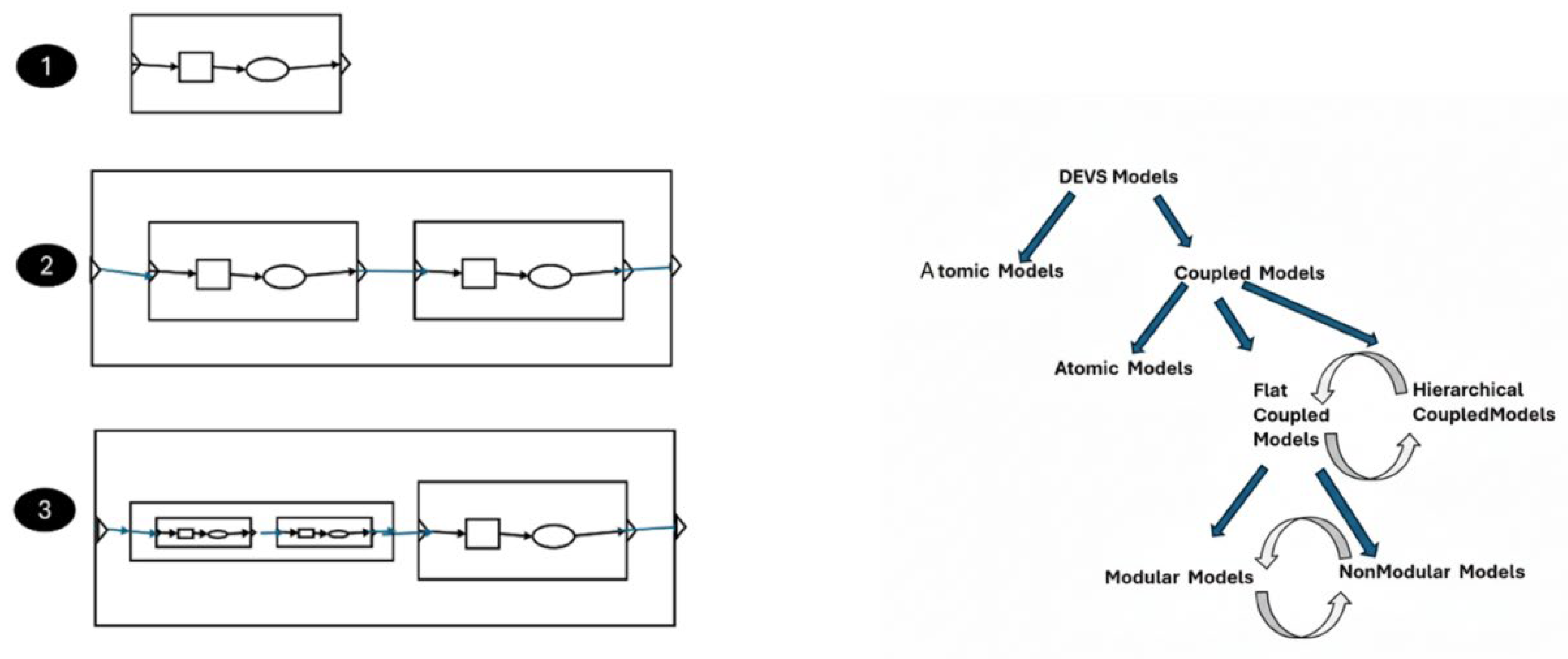
Figure 2.
a) Modelling and Simulation Framework, b) Experimental Frame in coupled model form.
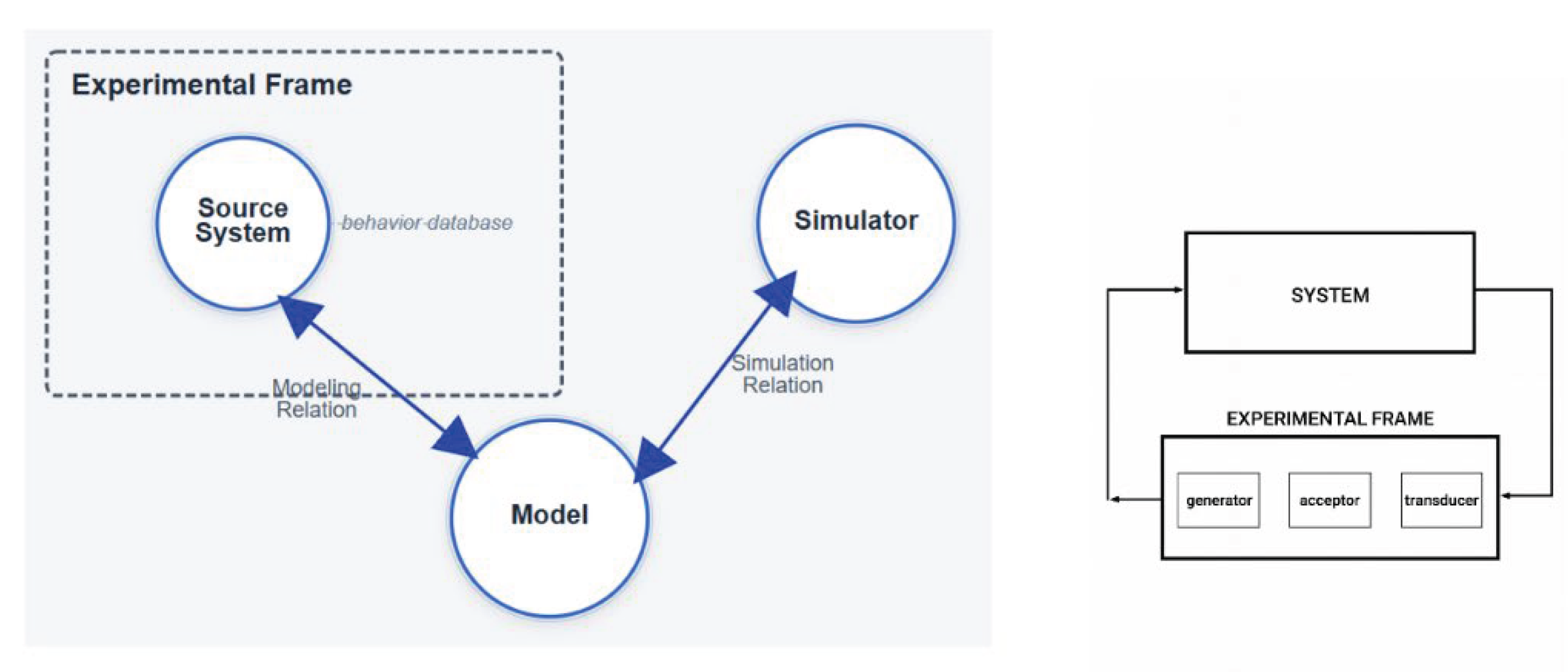
Figure 3.
a) DEVS-like systems exemplifying input and output time segments with discrete events, shown as vertical lines, b) DEVS representation of DEVS-like Systems at the levels of system specification ranging from input/output behavior to increasingly structural representations.
Figure 3.
a) DEVS-like systems exemplifying input and output time segments with discrete events, shown as vertical lines, b) DEVS representation of DEVS-like Systems at the levels of system specification ranging from input/output behavior to increasingly structural representations.
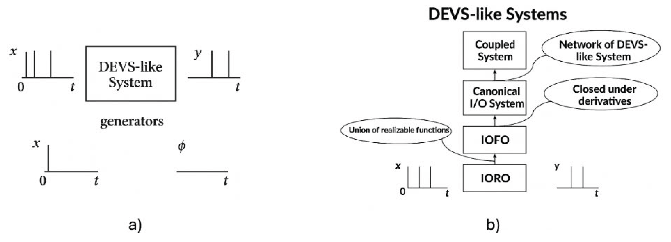
Figure 4.
Analogy: Geometric class of rectangles is closed under attachment, but the subclass of squares is not.
Figure 4.
Analogy: Geometric class of rectangles is closed under attachment, but the subclass of squares is not.
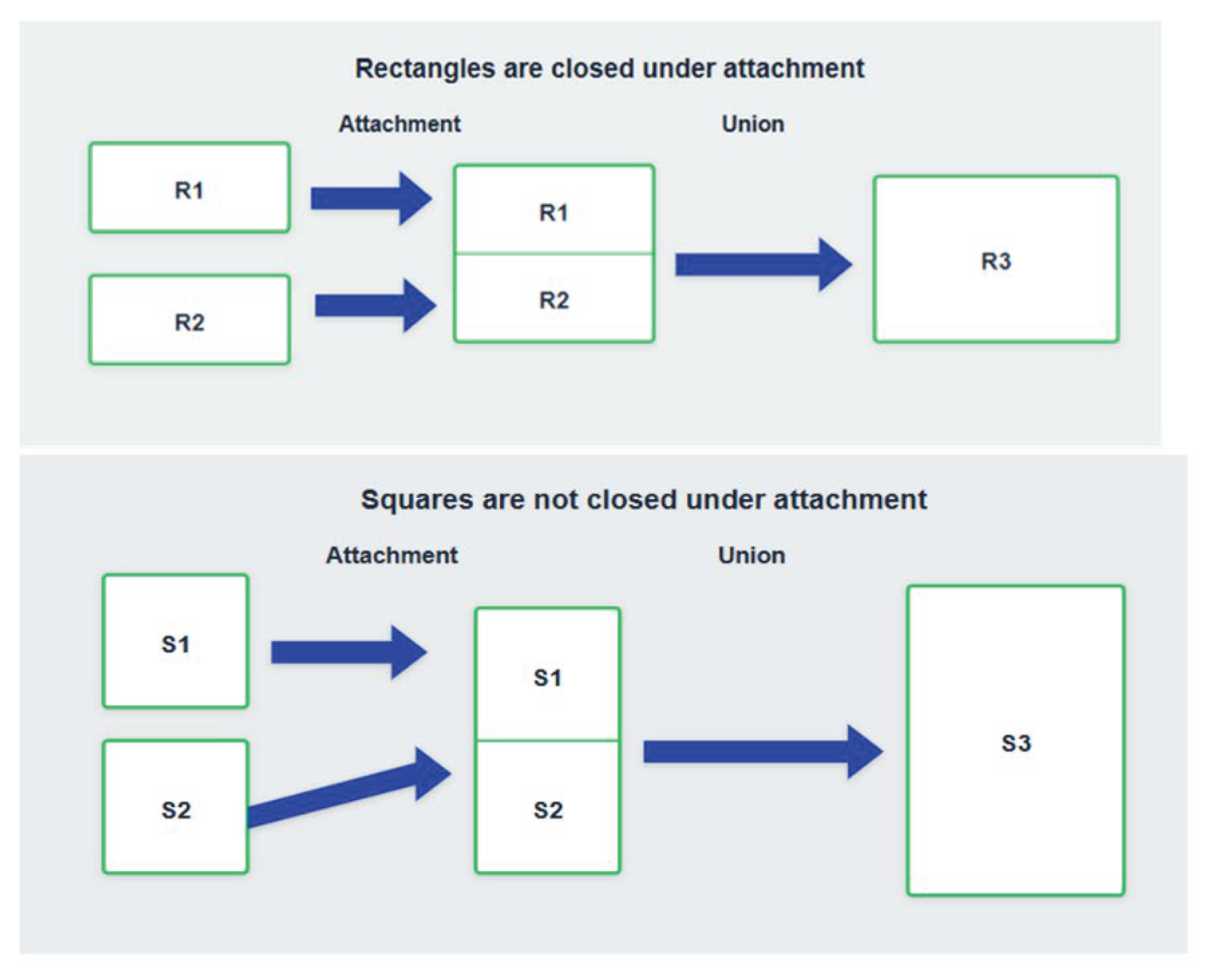
Figure 5.
Systems specification formulation of closure under coupling: a basic formalism (1) specifies (2) the subclass of Basic Systems; Coupled Subclass (3) specifies (4) Coupled Subclass Systems based on coupling (5) of Basic System Specifications. When closure under coupling holds, the resultant (6) is included in Basic Systems.
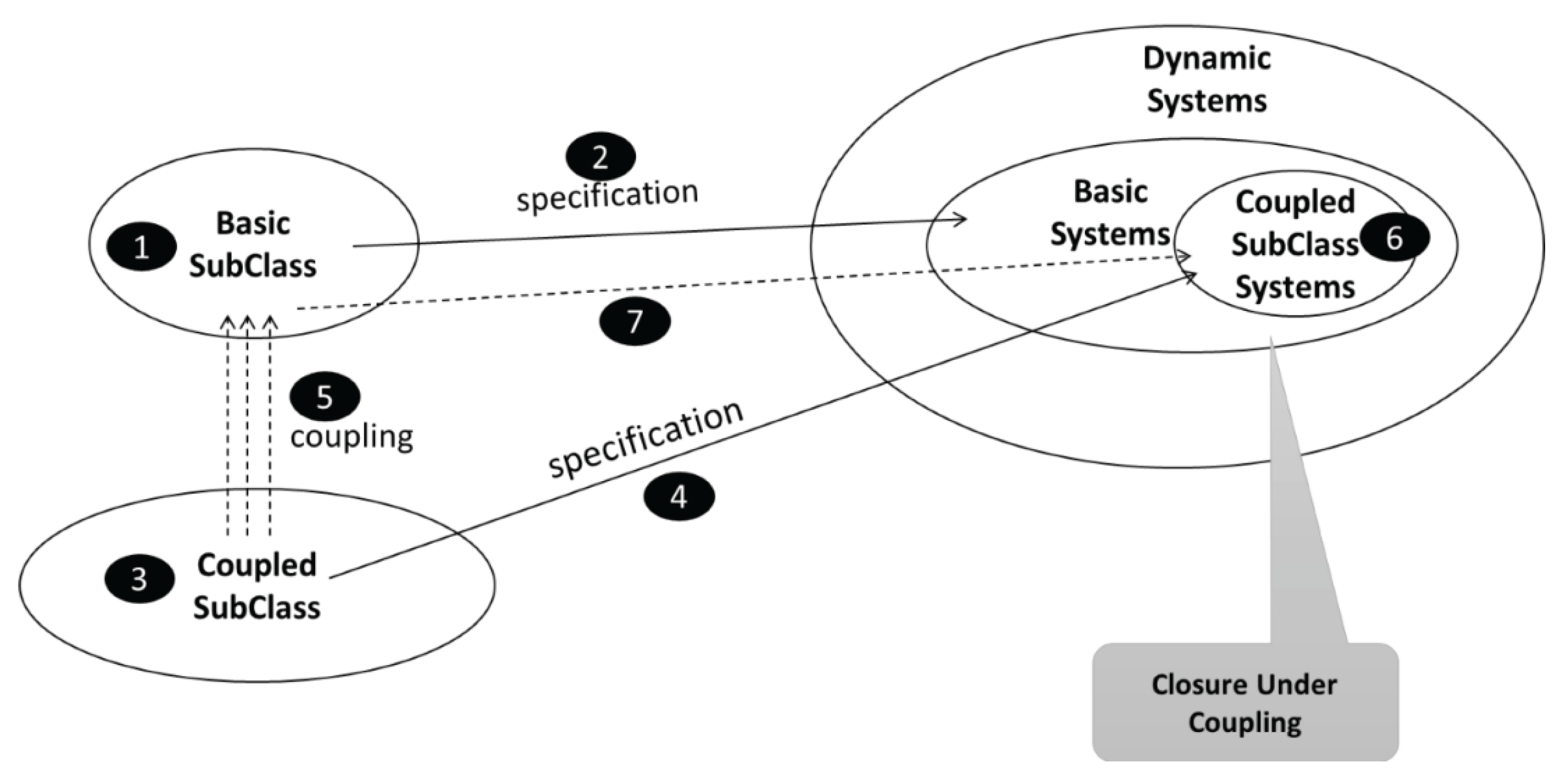
Figure 8.
a) UML class diagram sketch of DEVS Abstract Simulator, b) Illustrating Closure Atomic Class Structure.
Figure 8.
a) UML class diagram sketch of DEVS Abstract Simulator, b) Illustrating Closure Atomic Class Structure.
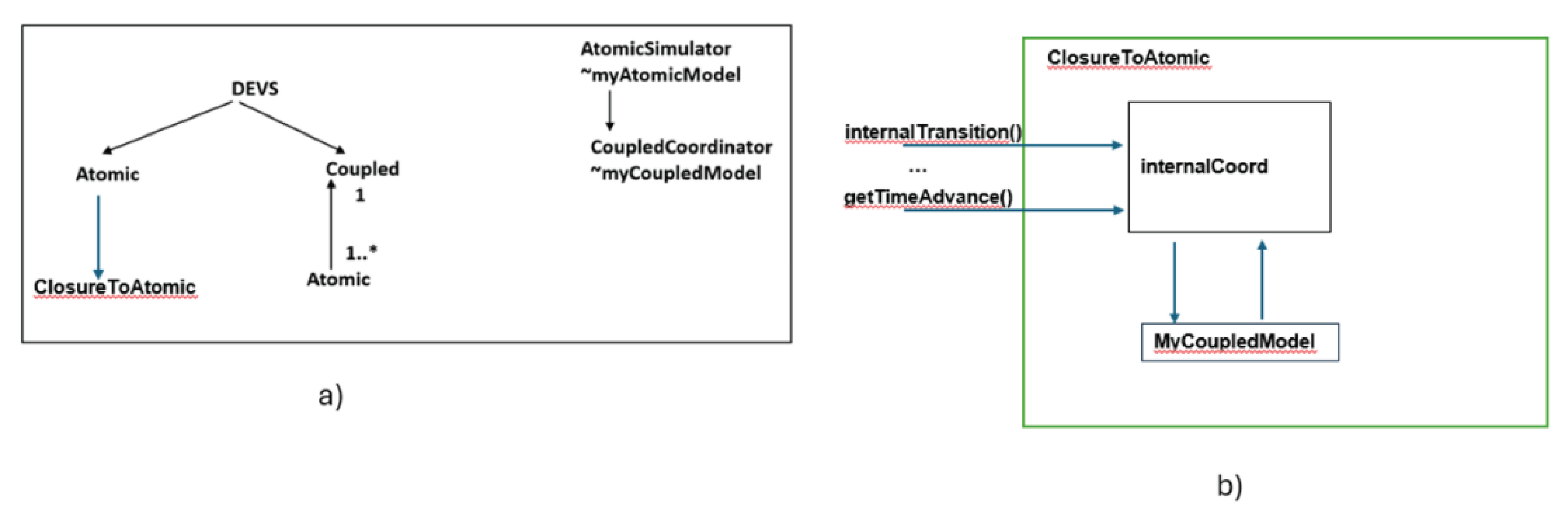
Figure 9.
DEVS BUS support of multiformalism modeling – originally defined for interoperating different event-scheduling “worldviews” and later generalized to different DEVS model specification formalisms.
Figure 9.
DEVS BUS support of multiformalism modeling – originally defined for interoperating different event-scheduling “worldviews” and later generalized to different DEVS model specification formalisms.
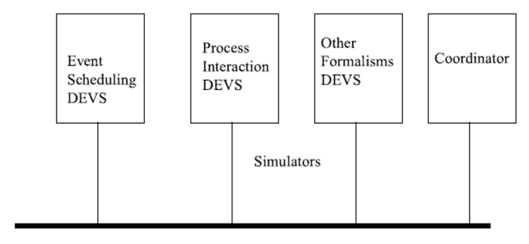
Figure 10.
Transforming Non-modular to Modular Structures. Transforming Non-modular to Modular Structures.
Figure 10.
Transforming Non-modular to Modular Structures. Transforming Non-modular to Modular Structures.
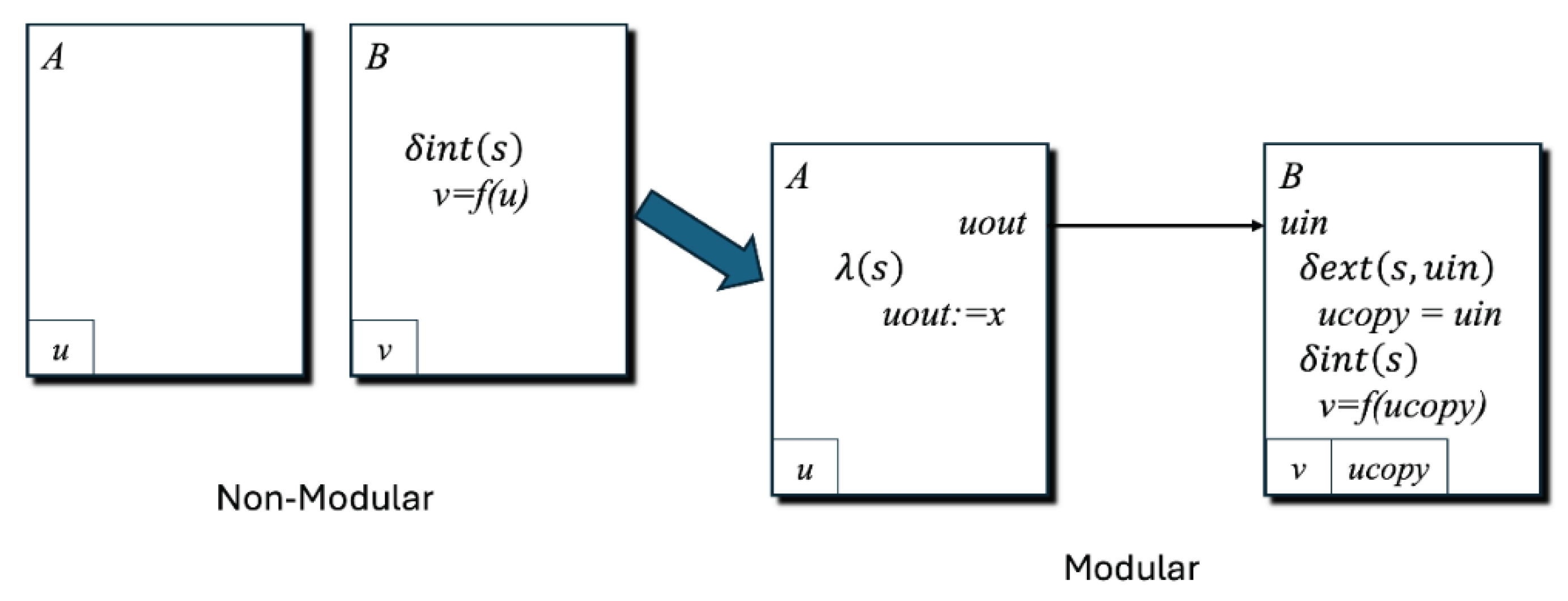
Figure 11.
Non-modular model illustrating direct access of B to A.
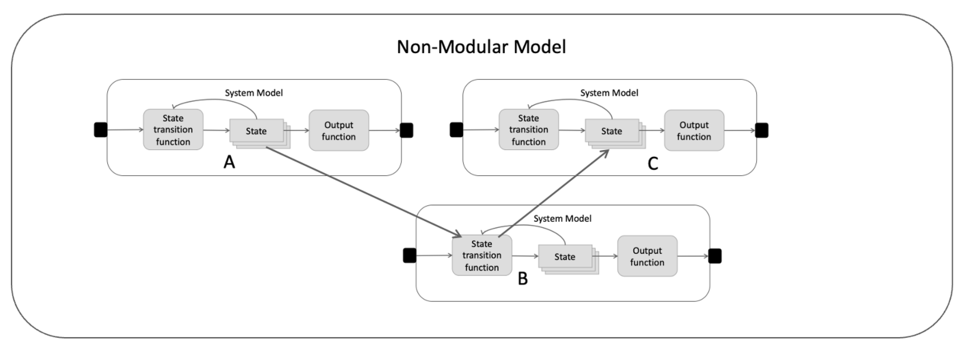
Figure 12.
Non-modular distributed simulation protocols. Non-modular distributed simulation protocols.
Figure 12.
Non-modular distributed simulation protocols. Non-modular distributed simulation protocols.
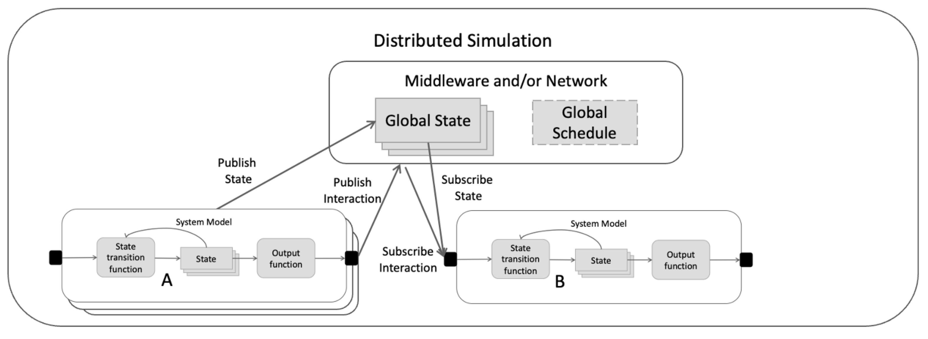
Figure 13.
Non-modular WebLVC model wrapped by a DEVS model.
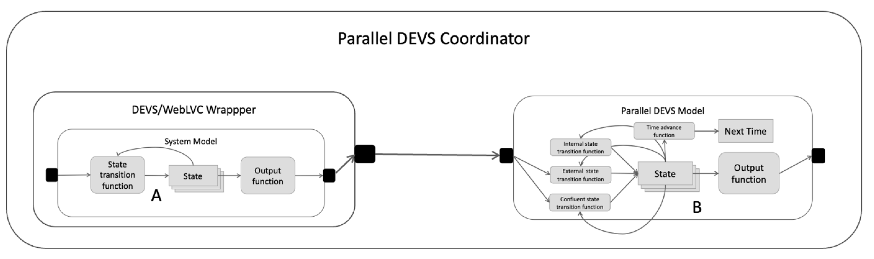
Figure 14.
UML diagram describing the libraries for modeling FMI based applications.
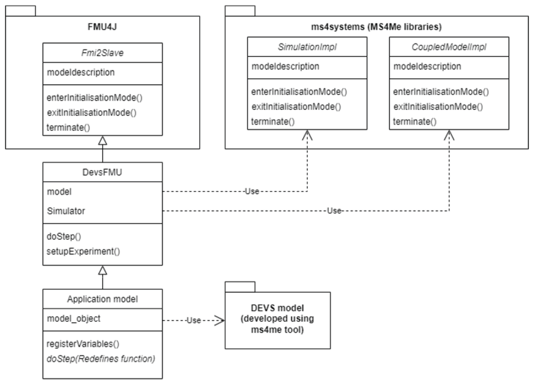
Figure 15.
Flattening Illustration a) Hierarchical Model (left) flattened (right) ; b) System entity structure representation, before and after flattening.
Figure 15.
Flattening Illustration a) Hierarchical Model (left) flattened (right) ; b) System entity structure representation, before and after flattening.
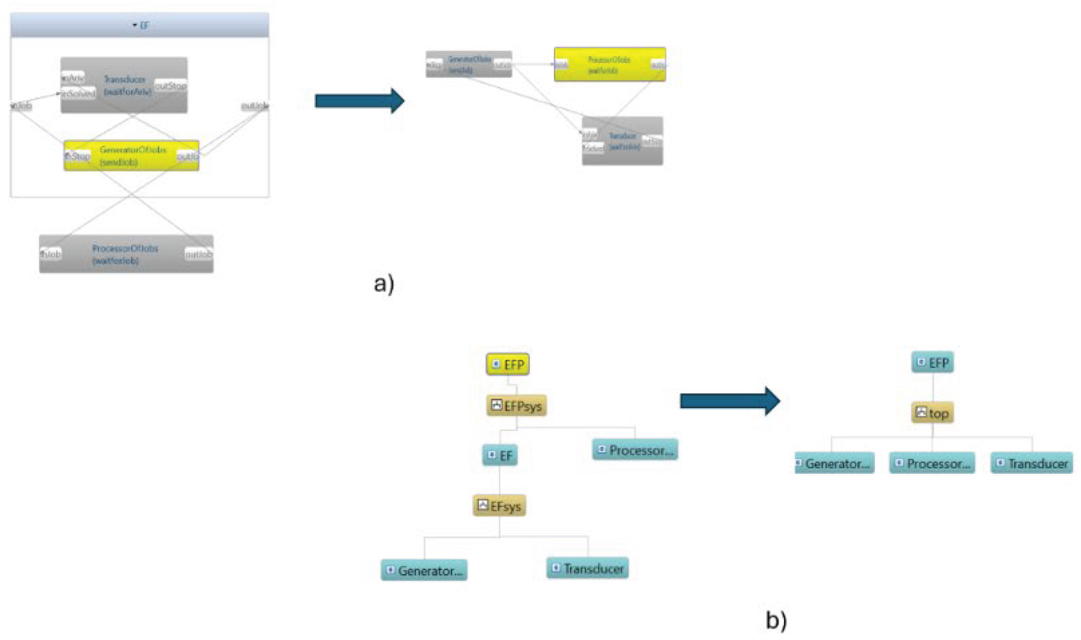
Figure 16.
Illustrating the basic step in the flattening operation; (top) in the original structure, component C1 sends message x to component C2 which transmits it to subcomponent C3, (bottom) in the flattened structure, component C1 sends message x directly to C3 which is now at the same level as C1 since C2 is eliminated and replaced by its children,.
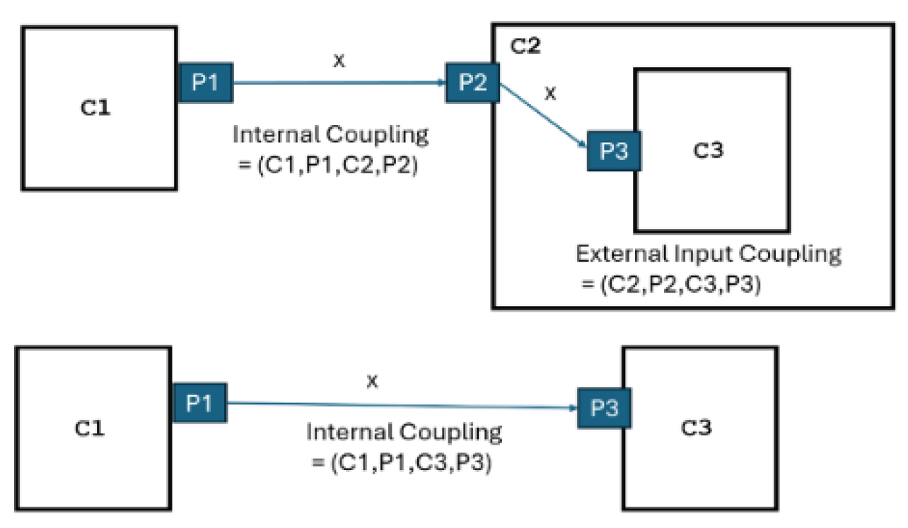
Figure 17.
Code Sketch for Flattening Operation on Coupled Models.
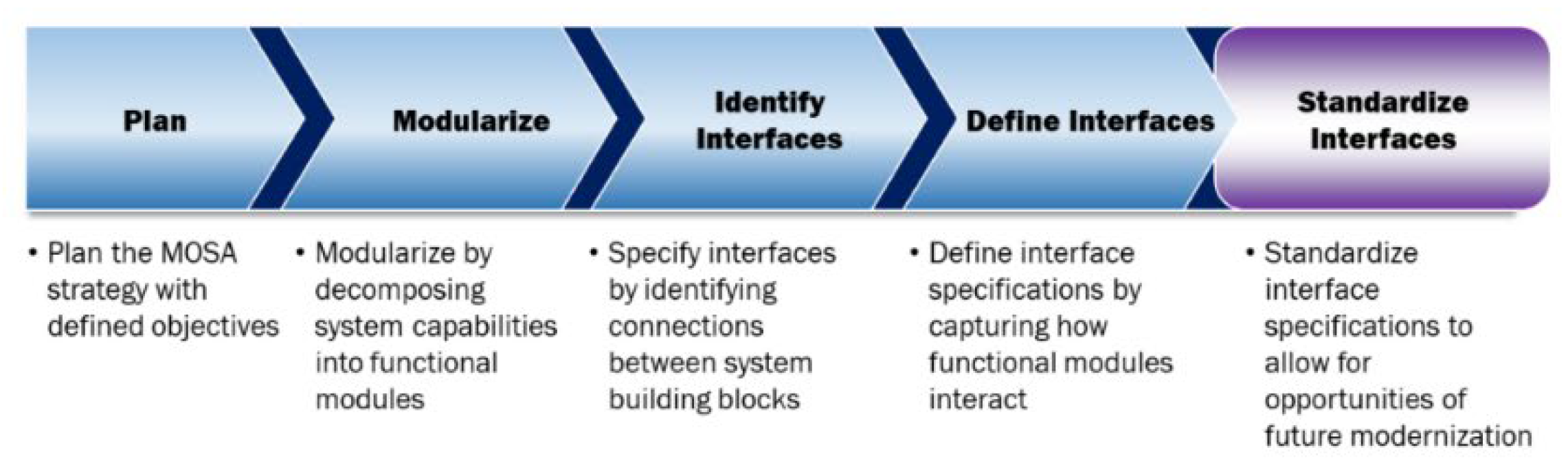
Figure 18.
MOSA Planning Framework.

Table 1.
Initial Global State of Model.
| Component | Sequential State | Time Advance |
|---|---|---|
| Imm (Imminent) | sendActivate | 1. |
| RecImm (Receives input and is Imminent) | sendActivate | 1. |
| RecNonImm (Receives input and is not Imminent) | waitForActivate | infinity |
| NonImm (NonImminent) | active | 10. |
Table 2.
Coupling Table for ClosureIllustrationExample.
| source | Outport | destination | inport |
|---|---|---|---|
| Imm | OutActivate | RecImm | inActivate |
| Imm | OutActivate | RecNonImm | inActivate |
| RecImm | OutActivate | NonImm | inActivate |
Table 4.
Definition Sketches of DEVS Functions.
| The wrapped model definition of the | Sketch of its definition |
|---|---|
| Internal transition function | 1) Get the next event time from the internal coordinator 2) Tell the internal coordinator to execute its next event at the given next event time |
| External transition function with arguments of elapsed time and input bag | 1) Get the last event time from the internal coordinator 2) Tell the internal coordinator to process the input bag with the time stamp of the given last event time plus the elapsed time |
| Output function | Tell the internal coordinator to compute the output and return this output bag |
| Time advance function | Tell the internal coordinator to get the next event time and the last event time and to return the second minus the first |
Table 5.
Application of DEVS Principles to MOSA. Application of DEVS Principles to MOSA.
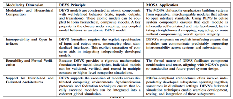 |
Table 6.
Drawbacks of Flattening.
| Aspect | Drawbacks |
|---|---|
| Information Retention | Loss of critical design information from intermediate models; less intuitive for human analysis. |
| Verification & Validation (V&V) | It is more difficult to gain insight during V&V; harder to quickly identify errors. |
| Visualization | Less data available for visualizations unless extra logging is added, which may slow performance. |
| Computation for Flattening | Flattening algorithms can be computationally expensive, especially for deep hierarchies. |
| Dynamic Structure Change | Complex to implement dynamic changes without original hierarchical location data. |
| Reusability | Reduced modularity makes components harder to reuse across models. |
| Parallel/Distributed Simulation | Partitioning for parallel/distributed execution is more complex; reduced modular boundaries hinder load balancing. |
| Design Intent | Requires supplementary metadata/annotations to convey original design intent. |
| Scalability | May create a combinatorially larger number of direct couplings, increasing memory and initialization costs. |
| Reconstruction of Hierarchy | Original modular structure cannot be uniquely recovered without comprehensive metadata. |
Table 7.
Deepening in Hierarchical Models — Benefits vs. Drawbacks.
| Aspect | Benefits of Deepening | Drawbacks of Deepening |
|---|---|---|
| Abstraction and Clarity | Groups related components into a higher-level coupled model, improving conceptual clarity and modularity. | May obscure fine-grained details, making debugging or tracing individual component behavior harder. |
| Reusability | Facilitates reuse of coupled subsystems as encapsulated modules in other models. | Over-encapsulation can reduce flexibility if frequent modifications to internal components are needed. |
| Maintainability | Simplifies top-level model structure by reducing the number of visible components. | Adds complexity to the hierarchy, requiring careful documentation to avoid confusion. |
| Scalability | Supports scaling by organizing large systems into manageable subsystems. | Excessive nesting can lead to deep hierarchies that are difficult to navigate and maintain. |
| Behavior Preservation | Coupling amendments ensure that the overall system behavior remains consistent after grouping. | Risk of introducing coupling errors or unintended side effects during restructuring. |
| Decision Support | Provides a structured view of system evolution, useful for teaching, analysis, and standards alignment. | May require additional reasoning steps to validate equivalence with the flattened version. |
Table 8.
Challenges in developing a DEVS standard for interoperable simulation modules.
| Type of Challenge | Description |
|---|---|
| Support for Experimental Frames | Support for specification of experimental frames is essential to facilitate the sharing, reuse, and management of DEVS models and simulation experiments within the modeling and simulation community, promoting collaboration and reducing redundant efforts. |
| Semantic Divergence | Variations in lifecycle semantics and behavior across DEVS implementations; lack of formal equivalence between DEVS variants (Classic, Parallel, etc.). |
| Platform & Language Interoperability | Diverse programming languages and environments complicate module exchange; middleware and adapter design must preserve DEVS semantics. |
| Tool Development & Infrastructure Gaps | Absence of unified model formats, graphical editors, and debugging tools limits usability and adoption across domains. |
| Testing & Certification | No standard benchmark suite or compliance criteria; distributed execution introduces synchronization and rollback complexities. |
| Community & Governance | Fragmented research communities and legacy systems resist change; balancing extensibility with strict interoperability is politically and technically complex. |
Disclaimer/Publisher’s Note: The statements, opinions and data contained in all publications are solely those of the individual author(s) and contributor(s) and not of MDPI and/or the editor(s). MDPI and/or the editor(s) disclaim responsibility for any injury to people or property resulting from any ideas, methods, instructions or products referred to in the content. |
© 2025 by the authors. Licensee MDPI, Basel, Switzerland. This article is an open access article distributed under the terms and conditions of the Creative Commons Attribution (CC BY) license (http://creativecommons.org/licenses/by/4.0/).
Copyright: This open access article is published under a Creative Commons CC BY 4.0 license, which permit the free download, distribution, and reuse, provided that the author and preprint are cited in any reuse.


