
Submitted:
14 October 2025
Posted:
16 October 2025
You are already at the latest version
Abstract
This paper presents a frequency analysis of annual maximum discharges for two river basins in Romania, using the Halphen-A distribution, which belongs to the Halphen family of distributions (including Halphen-B and Halphen-Inverse types). The distribution parameters were estimated using two distinct methods: the Method of Moments and the Maximum Likelihood Method. The results are compared with the Pearson Type III distribution, which is considered the reference distribution in Romania for statistical hydrology studies. The performance of each model was evaluated through a multi-criteria approach, employing the Root Mean Square Error (RMSE) and the Mean Absolute Error (MAE). The analysis highlights the advantages and limitations of each distribution and estimation method, providing a detailed perspective on the applicability of Halphen distributions in flood frequency hydrology.
Keywords:
extreme events
; Halphen
; Pearson III
; heavy-tail behavior
1. Introduction
The frequency analysis of annual maximum discharges plays a crucial role in hydrology, with direct implications for the design of hydraulic structures, flood risk management, and the development of adaptation strategies to climate change. In Romania, the Pearson Type III distribution is widely used in such studies, due to its flexibility in representing the characteristic skewness of extreme discharge series [1]. However, recent advances in probability distribution theory suggest that the Halphen family of distributions may provide a more accurate representation of hydrological data because of its more flexible parameterization and ability to model a wider range of skewness and kurtosis values.
The aim of this study is to compare the performance of Halphen distributions with that of the Pearson Type III distribution in modeling annual maximum discharges for two representative case studies from Romania. The comparison seeks to evaluate not only the statistical goodness of fit but also the physical interpretability and robustness of parameter estimates across different estimation methods. Through this analysis, the study contributes to a better understanding of the potential advantages of Halphen-type models in frequency analysis and their applicability in modern hydrological practice and water resources engineering.
2. Materials and Methods
The Halphen family of distributions was initially introduced in engineering and geostatistical applications but has recently gained attention in hydrological analysis due to its remarkable flexibility in modeling asymmetric distributions [2,3,4].
This family includes three main types:
- -
- Halphen-A (HA) distribution, suitable for series exhibiting moderate skewness and long tails.
- -
- Halphen-B (HB) distribution, capable of modeling highly skewed series, often applied when data show a significant deviation from normality.
- -
- Halphen-Inverse (HI) distribution, appropriate for datasets with pronounced extreme values and a high concentration of probability in the lower part of the distribution.
The major advantage of the Halphen distributions lies in their ability to adapt to various shapes of extreme-value data, making them strong competitors to classical models such as the Generalized Extreme Value [5], Pearson Type III [1], or Log-Pearson Type III distributions. Their flexible parameterization allows for the simultaneous representation of different statistical characteristics (mean, variance, skewness, and kurtosis) in a unified mathematical framework, which can lead to more accurate modeling of hydrological extremes, especially under non-stationary conditions.
A crucial aspect of frequency analysis is the method used to estimate the parameters of the chosen probability distribution. In this study, two main estimation methods are analyzed and compared:
- -
- Method of Moments (MOM), one of the simplest and most intuitive approaches, based on equating the sample moments to the theoretical moments of the distribution. Although computationally straightforward, it can be sensitive to outliers and the sample size, which may affect parameter stability.
- -
- Maximum Likelihood Estimation (MLE), a statistically rigorous method that determines parameters by maximizing the likelihood function. It typically yields efficient and asymptotically unbiased estimates for large samples, but it is computationally more complex and sensitive to the assumptions of data independence and identically distributed samples.
By applying both estimation methods to the Halphen and Pearson III distributions, the study aims to highlight the strengths and weaknesses of each approach in capturing the statistical behavior of extreme hydrological events, ultimately contributing to a better understanding of their applicability in flood frequency modeling and risk assessment.
If a random variable X follows a Halphen-A distribution, the probability density function with parameters,, and is defined by [2,3,4]:
The complementary cumulative distribution function is:
3. Case Study
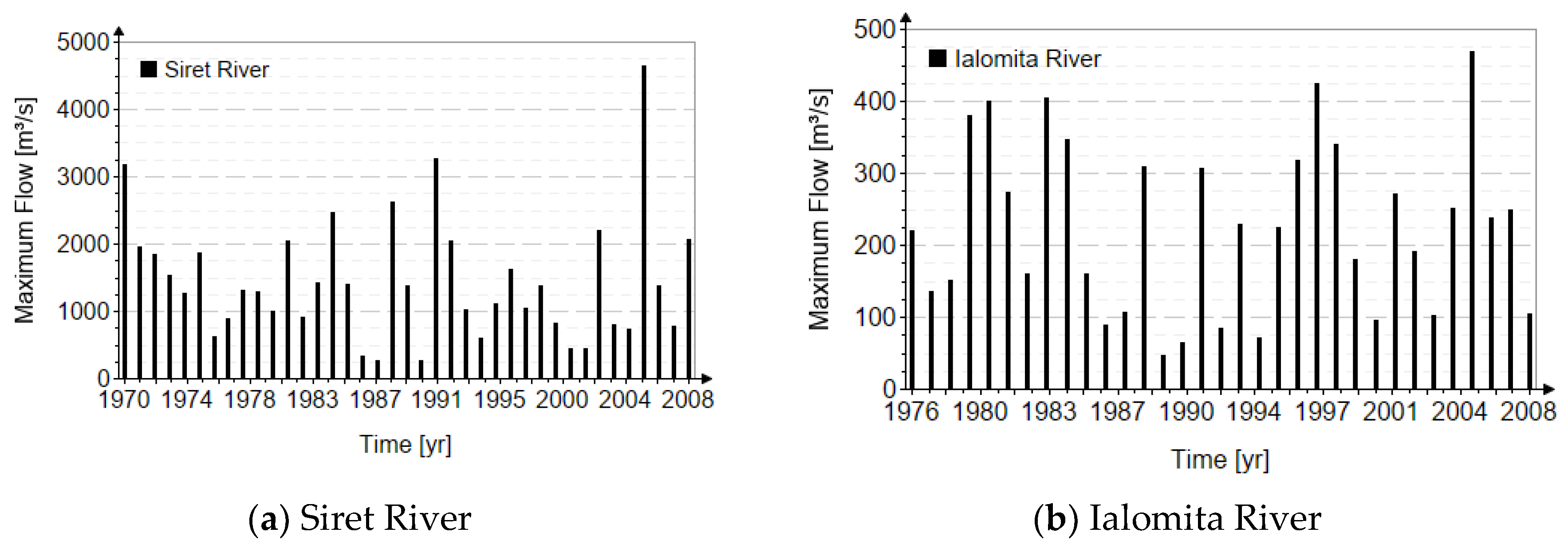
The two case studies consist of performing frequency analyses of maximum flows based on the annual maximum flow series on the Ialomita and Siret rivers, two data series chosen as reference in the Romanian regulations [6].
The statistical indicators for the analyzed sites are summarized in Table 1.
Taking into account the relatively short lengths of available data, the skewness was established according to Romanian practices, namely multiplying the coefficient of variation by a factor that depends on the origin of the maximum flows. In both cases, the coefficient chosen 2.
Figure 1.
The annual values of maximum discharges.
4. Results
The quantile function curves obtained for both case studies (Figure 2) reveal that the Halphen-A and Pearson III distributions provide very good agreement with the observed discharge data. For the Siret River (Lungoci station), both distributions captured the empirical behavior well, particularly in the upper quantile range corresponding to high return periods.
The MOM and the MLE yielded very similar fitted curves, with the Halphen-A slightly outperforming Pearson III for higher flows.
For the Ialomița River (Țăndărei station), the two distributions exhibited almost identical results for the lower and medium quantiles, while small differences were observed for the upper tail. Again, the Halphen-A model proved slightly more flexible, showing a smoother transition in the tail zone, which can be advantageous in extrapolating to rare events.
Quantitatively, the model performance was assessed using RMSE and MAE, as summarized in Table 2 and Table 3. For both rivers, the error values were very low, confirming the robustness of both models. The Halphen-A distribution estimated by MLE achieved the smallest RMSE and MAE for the Siret River (0.0042 and 0.0224), while for the Ialomița River, the lowest values corresponded to the Halphen-A (MLE) as well (0.0080 and 0.0373). These results highlight the excellent consistency and numerical stability of the Halphen-A model across different estimation methods.
5. Discussions
The comparative analysis between the Halphen-A and Pearson III distributions demonstrates that both are suitable for hydrological frequency analysis in Romanian conditions. However, the Halphen-A distribution offers a higher degree of flexibility in shape due to its three-parameter structure, enabling it to model a broader range of skewness and kurtosis values. This flexibility is particularly valuable for basins exhibiting heterogeneous hydrological behavior or limited data length, as in the current study.
From a methodological point of view, the MLE generally provided slightly better results than the MOM, as reflected by the lower RMSE and MAE values in both case studies. This confirms the theoretical expectation that MLE yields more efficient estimates, especially when the underlying distributional assumptions are approximately met. Nevertheless, the MOM remains a practical alternative for small samples or when computational simplicity is preferred.
The results also indicate that the Halphen-A distribution tends to produce smoother quantile curves and reduced tail bias, particularly for the largest return periods (T > 50 years). This property could be essential for flood frequency analysis under non-stationary or data-scarce conditions. On the other hand, the Pearson III distribution continues to provide robust results, confirming its long-standing reliability and its historical role as the “parent distribution” in Romanian hydrology.
Overall, the study supports the view that Halphen-type models can complement or even improve upon traditional distributions such as Pearson III, particularly in applications involving heavy-tailed hydrological data or skewed flood series.
6. Conclusions
The comparative analysis performed on the Siret and Ialomița rivers leads to the following main conclusions:
- -
- Both the Halphen-A and Pearson III distributions provide satisfactory fits to annual maximum discharge data, with very low RMSE and MAE values, confirming their applicability in hydrological frequency analyses.
- -
- The Halphen-A distribution, due to its flexible parametrization, exhibits a slightly superior capability to reproduce the empirical shape of the quantile function, especially in the upper tail of the distribution.
- -
- Between the two parameter estimation methods, the MLE consistently yielded lower errors and more stable parameter estimates than the MOM.
- -
- The Halphen-A distribution can be confidently used as an alternative or complementary model to Pearson III in Romanian hydrological practice, particularly in basins with strong asymmetry or limited data length.
- -
- The results encourage the integration of Halphen distributions into national and regional flood frequency analyses, potentially improving the precision of design flood estimations and supporting better risk-informed decision-making in water resources management.
References
- Anghel, C.-G.; Ianculescu, D. An In-Depth Statistical Analysis of the Pearson Type III Distribution Behavior in Modeling Extreme and Rare Events. Water 2025, 17, 1539. [Google Scholar] [CrossRef]
- El Adlouni, Salah-Eddine; Chebana, Fateh et Bobée, Bernard (2010). Generalized Extreme Value versus Halphen System: Exploratory Study. Journal of Hydrologic Engineering , vol. 15 , nº 2. pp. 79-89. [CrossRef]
- Dvorák, Václav; Bobée, Bernard; Boucher, Sylvie et Ashkar, Fahim (1988). Halphen distributions and related systems of frequency functions. Rapport scientifique (R236). INRS-Eau, Québec.
- Perreault, L. & Bobée, Bernard & Rasmussen, Peter. (1999). Halphen Distribution System. I: Mathematical and Statistical Properties. Journal of Hydrologic Engineering - J HYDROL ENG. 4. [CrossRef]
- Anghel, C.G.; Ianculescu, D. Application of the GEV Distribution in Flood Frequency Analysis in Romania: An In-Depth Analysis. Climate 2025, 13, 152. [Google Scholar] [CrossRef]
- The Regulations Regarding the Establishment of Maximum Flows and Volumes for the Calculation of Hydrotechnical Retention Constructions; Indicative NP 129-2011; Ministry of Regional Development and Tourism: Bucharest, Romania, 2012.
Figure 2.
The quantile function curves corresponding to the analyzed probability distribution.
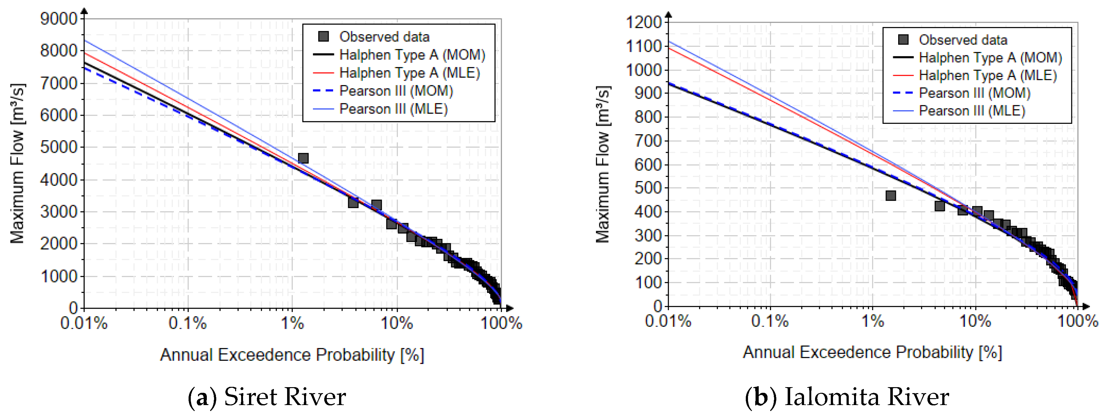

Table 1.
Statistical indicators of the observed data.
| River/Station | (kurtozis) | ||||
|---|---|---|---|---|---|
| [m3/s] | [-] | [-] | [-] | [-] | |
| Siret/Lungoci | 1442.5 | 0.634 | 0.379 | 1.269 | 7.872 |
| Ialomita/Tandarei | 224.1 | 0.527 | 0.327 | 1.054 | 4.074 |
Table 2.
RMSE and MAE score values for the Ialomita River.
| Ialomita River | ||||
|---|---|---|---|---|
| Distribution | MAE | RMSE | ||
| MOM | MLE | MOM | MLE | |
| Halphen-A | 0.0404 | 0.0373 | 0.0085 | 0.008 |
| Pearson III | 0.0404 | 0.0383 | 0.0085 | 0.0082 |
Table 3.
RMSE and MAE score values for the Siret River.
| Siret River | ||||
|---|---|---|---|---|
| Distribution | MAE | RMSE | ||
| MOM | MLE | MOM | MLE | |
| Halphen-A | 0.021 | 0.0224 | 0.00399 | 0.0042 |
| Pearson III | 0.0203 | 0.0278 | 0.00395 | 0.0052 |
Disclaimer/Publisher’s Note: The statements, opinions and data contained in all publications are solely those of the individual author(s) and contributor(s) and not of MDPI and/or the editor(s). MDPI and/or the editor(s) disclaim responsibility for any injury to people or property resulting from any ideas, methods, instructions or products referred to in the content. |
© 2025 by the authors. Licensee MDPI, Basel, Switzerland. This article is an open access article distributed under the terms and conditions of the Creative Commons Attribution (CC BY) license (http://creativecommons.org/licenses/by/4.0/).
Copyright: This open access article is published under a Creative Commons CC BY 4.0 license, which permit the free download, distribution, and reuse, provided that the author and preprint are cited in any reuse.


