
Submitted:
13 October 2025
Posted:
15 October 2025
You are already at the latest version
Abstract
This paper proposes the novel application of group counterfactual explanations to the problem of predicting student at risk of drop-out. Our objective is to provide explanations for trying to re-cover the largest number of students with less effort and cost. Using group counterfactuals, in-structors and institutions could recover large groups of students with minimal remedial actions. For testing it, we have used the well-known public educational OULAD dataset that contains student’s clicks made throughout interaction with online courses. We have modified and adapted the only existed algorithm for generating group counterfactual named GROUP-CF. We also used the DICE individual counterfactual algorithm with the K-means clustering method and new op-tions for discovering the most representative counterfactuals for a group of students. The results obtained are very promising and they show that our approach can be successfully applied to re-cover 99.3% of students at risk of failing in a shorter time in comparison to traditional individual counterfactuals. And although, a group counterfactual proposes to change a greater number of student’s features, the values are lighter and therefore seem easier to apply than the ones obtained with individual counterfactuals. This work opens a new line of research in education.
Keywords:
XAI
; counterfactual explanations
; group explanations
; at risk of failure
1. Introduction
In the current era of rapidly expanding real-world AI applications, the transparency and interpretability of Machine Learning (ML), Data Mining (DM), and Deep Learning (DL) models have become critical. But often, these models are considered ‘black boxes’ because of the difficulty in understanding the reasons behind their decisions [1]. This lack of clarity is of particular concern in sectors where automated decisions have a significant impact on people's lives, such as education, health or finance. In this context, Explainable Artificial Intelligence (XAI) has emerged as a key discipline, seeking to unravel the inner workings of ML models and provide clear and understandable explanations for end users. One of the most prominent approaches in the field of XAI is the generation of counterfactual scenarios or explanations [2]. These are hypothetical scenarios that show the reality of what would have happened if other decisions had been made. Counterfactuals provide an intuitive way to understand how small changes in a model's inputs can change its decisions. For example, a counterfactual scenario might answer the question: ‘What should be different in the student X’s learning behavior so that she would not be predicted as at risk of dropping out?”. This ability to provide clear, action-oriented explanations has led counterfactuals to feature prominently in the XAI literature and especially in the education domain [3]. Additionally, the current increasing interest in generating counterfactual scenarios arises not only because of their easy interpretability, but also because various legal analyses suggest that these counterfactual scenarios meet the requirements of the GDPR (General Data Protection Regulation), as they allow providing clear and understandable explanations of automated decisions without compromising the privacy of individuals [4].
However, all research and applications of counterfactuals focus on individual scenarios, i.e. each instance receives a unique prediction and explanation. This approach, while useful for each particular instance or student, does not address cases where multiple instances or students may share common characteristics and thus benefit from a group counterfactual scenario. The generation of group counterfactuals allows for the creation of a single explanation for a set of similar instances or students, facilitating the identification of patterns and promoting efficiency in decision-making. They are only a few works that deal with the general problem of generating group counterfactual and try to provide more informative about patterns than individual counterfactuals [5]. This less study type of counterfactual poses psychological advantages because it reduces stakeholders’ memory load and facilitates pattern-finding [6].
In the domain of education, group counterfactuals may have endless applications. For example, a group of students with similar academic characteristics could benefit from the same counterfactual explaining how to prevent academic failure, rather than generating a separate explanation for each student. Academic failure is a major challenge these days since it may have highly negative effects for educational institutions and students [7]. The identification of students at risk of academic failure is essential for timely instructional interventions [8,9], since students who fail at some point during their studies are 4.2 times more likely to dropout and leave their educational institutions [10]. There are many causes behind academic failure, among which we can find some related to aspects such as time management, family, learning, assessment, and subjects [11]. Some authors have recognized that uncooperative and hostile environments can lead to academic failure, and have linked it to low motivation, low engagement and alienation from school, suggesting that positive relations with teachers can thus be a protective factor against academic failure [12]. In addition, early academic failure, recently treated in the literature [13], can lead to consequences such as limited job opportunities, increased risk of unemployment, inequality and cycle of poverty, lower income, barriers to personal development, increased risk of social problems and even impact on health and well-being. It is essential to recognize the consequences of early school leaving and to work towards the implementation of education policies and programs that promote school retention, support at-risk students and promote equal educational opportunities.
The main contribution of this paper is the proposal of a framework for generating group counterfactual scenarios in the domain of education. The purpose is to identify common patterns among students at risk of failing and provide explanations and recommendations that can guide more effective interventions to help teachers support these at-risk students. Note that this approach does not intend to eliminate individualized types of interventions, sometimes indispensable in education, but to provide a complementary tool approach when stakeholders need or prefer group-focused interventions. Also note that this paper only addresses the generation of those group counterfactuals, but not their translation into effective actions derived from them to be applied by educators, which would be a topic for another research. Finally, in order to validate our framework, we have defined the next two research questions:
- • RQ1: Is it feasible to generate successful group counterfactuals for the problem of recovering at-risk of failing students at a reasonable time?
- • RQ2: What is the performance of group counterfactuals explanations compared to individual counterfactuals according to standard indicators in this problem?
To answer those RQs, we have developed a comprehensive validation process using a public educational dataset and from a quantitative perspective that complement the mostly qualitative validation performed by Warren and colleagues. As described at the end of the paper, the results obtained from this validation process indicate that our approach can be successfully applied to generate useful group counterfactuals explanations in our reference problem. These results show some clear advantages over individual counterfactuals in terms of execution time and the number of changes to be implemented in features for recovering at-risk students from failing into not failing.
The rest of the manuscript is structured as follows: section 2 presents the background of this work, and the literature related to it; the use case is presented in section 3; section 4 presents the validation of the proposed approach; finally, section 5 summarizes the conclusions and presents some future lines to be addressed.
2. Background
There are three related areas with our problem: counterfactual explanations, counterfactual in education and group counterfactuals.
2.1. Counterfactual Explanations
Counterfactuals are hypothetical scenarios or alternative situations that illustrate how outcomes might have been if a specific event or intervention had not taken place. They allow to answer questions such as: ‘What would have happened if instead if a certain feature took the value “x” instead of “y”?’ Counterfactuals are particularly useful when randomized controlled experiments, considered the ‘gold standard’ for establishing causal relationships, are not possible. Instead, observational studies and causal analysis algorithms are used to identify and evaluate counterfactuals [14].
In recent years, different methods have been developed for generating (individual) counterfactual explanations. Some of the most representative ones are Propensity Score Matching - PSM [15], Difference-in-Differences – DID [16], Regression Discontinuity - RD [17], and Instrumental Variable – IV [18], as well as other based on axiomatic attribution [4] and multi-objective minimization ideas [19].
However, the most popular method is DiCE, which stands for Diverse Counterfactual Explanations [20]. It is a post-hoc explainability tool designed to generate diverse counterfactual explanations for machine learning models. Unlike other methods which focus on assessing the importance of features in individual predictions, DiCE focuses on creating alternative scenarios (known as ‘what-ifs’) in which the model's predictions would change if certain attributes of the input were altered, making it easier to interpret for those without prior computational knowledge. Another difference with most existing methods is that, while they seek to generate explanations through the importance of variables or the visualization of graphs, DiCE seeks to generate explanations through examples, which is considered the most relevant way of generating explanations. An example of an explanation generation framework with DiCE is MMDCritic [21], which selects both prototypes and critiques from the original data points.
More recently, explanations are being proposed as a way to provide alternative perturbations that would have changed the prediction of a model [22]. In other words, given an input feature x and the corresponding output of a ML model f, a counterfactual explanation is a perturbation of the input to generate a different output y using the same algorithm. In most existing methods, the objective is to find a counterfactual explanation that minimizes both the distance to the original instance x and the loss associated with not achieving the desired prediction y. This is the standard process, which normally looks for a single counterfactual close to the original entry point that can change the decision of the model. However, the approach used in DiCE is different and focuses on generating a set of counterfactuals that not only change the decision of the model but also offer various alternatives for the user.
2.2. Counterfactuals in Education
Counterfactuals have been increasingly applied in education to improve interpretability, decision-making, and intervention design, no prior review has systematically examined their methodological, algorithmic, and presentation aspects within this domain. Counterfactual explanations can be applied in the educational field to answer important questions. For example, what should be the value of a specific characteristic/variable/factor for a student to move from being at risk of dropout to not being at risk? [23]. Understanding the interaction of factors to identify a student as at risk of dropout could help decision-makers interpret the situation and determine the necessary corrective actions to reduce or eliminate this risk [24].
Most of the research on counterfactual in education focuses on predicting academic performance, predicting student dropout, and improving learning outcomes. For instance, studies by Tsiakmaki and Ragos [25], Smith et al. [26], and Afrin et al. [27] use counterfactuals to identify small, actionable changes that could turn a failing prediction into a passing one. Similarly, Swamy et al. [28] and Garcia-Zanabria et al. [24] apply counterfactual reasoning to detect dropout risks and design targeted interventions, while other studies explore broader challenges such as fairness in admissions or optimizing cognitive learning experiences [29,30]. Collectively, these works demonstrate that counterfactuals not only improve the interpretability of AI models but also foster data-driven decision-making and personalized educational interventions.
About the specific methods and algorithms used when generating counterfactuals in education, it is possible to identify three main categories: optimization-based, instance-based, and heuristic search categories following Guidotti [2]. Optimization-based methods, such as Diverse Counterfactual Explanations (DiCE) and Contrastive Explanation Method (CEM), are the most common, focusing on balancing validity, proximity, diversity, and sparsity. Instance-based approaches (e.g., NICE and CORE) identify similar real examples in the data to construct plausible counterfactuals, while heuristic approaches like MOC rely on genetic algorithms to find optimal solutions. Additionally, several studies explore causality-aware methods, such as the Path-Specific Counterfactual (PSC) [29] and Structural Causal Models (SCM) [31], which explicitly model cause-effect relationships among educational factors. The authors highlight emerging research integrating Large Language Models (LLMs) and Generative Adversarial Networks (GANs) for counterfactual generation [32,33], as well as the use of group-based and path-based counterfactuals, which could help design more interpretable and context-aware educational interventions.
An important problem when generating counterfactual in education is how counterfactuals are presented to stakeholders. The way these findings are presented can influence the interpretation and comprehension of the results by the audience, including their capacity to discern major patterns and trends. There are five main forms or presenting counterfactuals in education: textual, tabular, visual static, visual interactive, and flow/process-based presentations. Textual explanations (e.g., Afzaal et al. [34]; Ramaswami et al. [35]) use natural language to provide recommendations, while tabular formats [25,36] organize feature changes systematically. Visual static forms (e.g., [29]) include graphs and causal diagrams, whereas interactive dashboards [24,37] enable users to explore counterfactual outcomes dynamically. The authors argue that integrating multiple presentation modes — textual for interpretability, visual for clarity, and interactive for engagement — can significantly improve how educators understand and apply counterfactual insights in practice. However, they note that many studies still lack advanced visualization or user-centered presentation approaches.
So, counterfactual explanations hold significant potential to transform educational analytics, promoting transparency, fairness, and personalized learning. Some current research challenges and directions for future work are: integrating prescriptive analytics and personalized feedback, extending counterfactual reasoning to underexplored areas such as student motivation and engagement, incorporating causal inference and reinforcement learning, and designing interactive, multimodal visualization frameworks. While current research demonstrates substantial progress, the educational field of applying/generating counterfactual is still in the early stages of fully harnessing counterfactual reasoning to support informed, equitable, and actionable decision-making.
2.3. Group Counterfactuals
Given the recent boom in artificial intelligence, there are still few papers related to the generation of (individual) counterfactuals and even fewer when it comes to group counterfactual generation. To the best of our knowledge, there is only one paper proposing an algorithm for generating group counterfactuals, proposed by Warren et al. [5]. The main objective is to provide users with an understanding of how the model decision would change if certain characteristics of the group were modified, which is particularly relevant in scenarios where decisions collectively affect multiple instances or users.
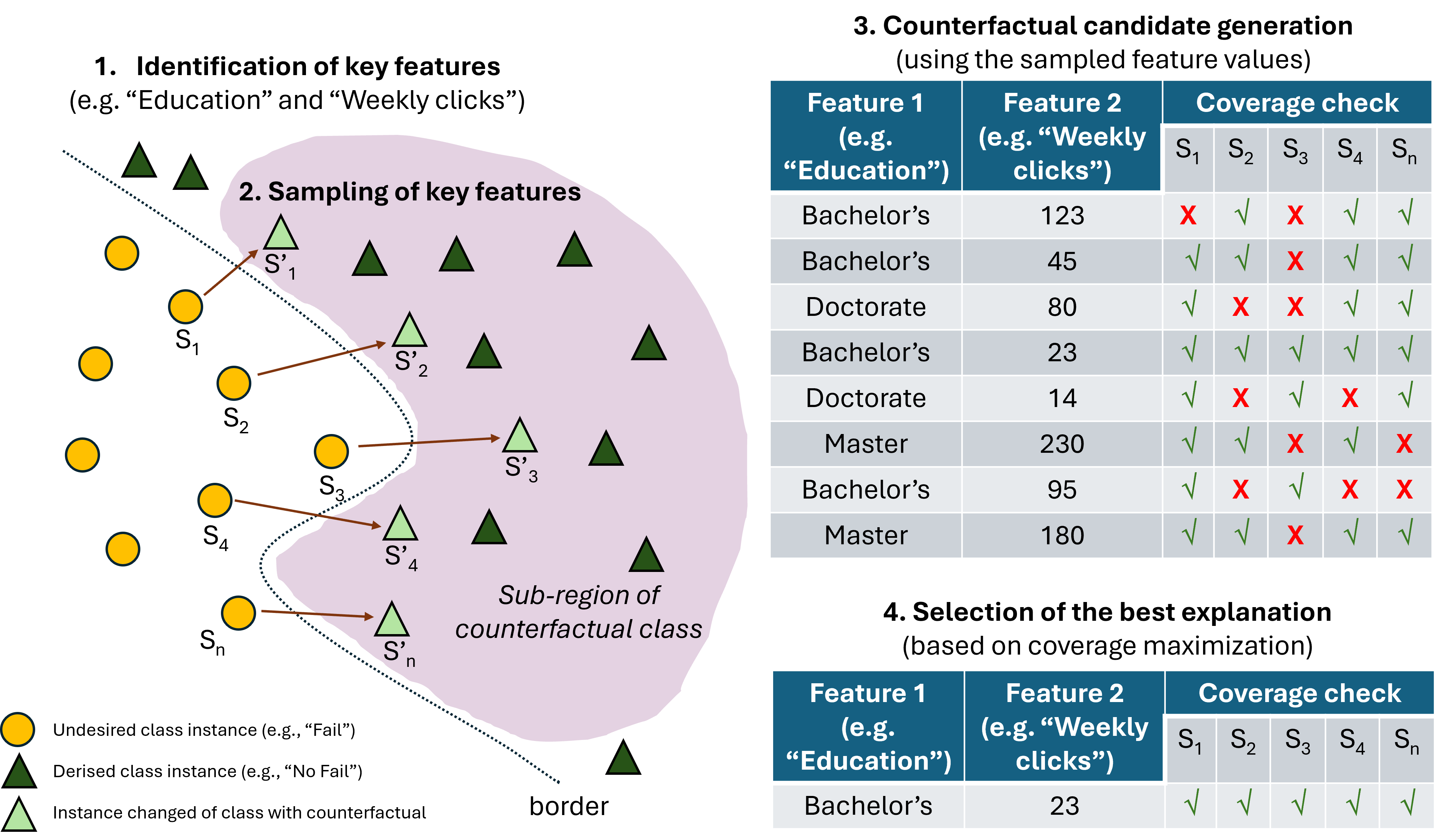
In order to generate these group counterfactuals, Warren et al. [5] developed an algorithm whose starting point is a set of related instances that have been classified by the model as being of the same class. Taking these inputs, the four main steps of the method are as follows:
- Identification of key features: For each instance, multiple individual counterfactual explanations are generated using DiCE. They then analyze the differences in features that produce the classification change in these individual counterfactuals, identifying those features that are most effective in altering the model's prediction. Those features are candidates for being included in the group counterfactuals.
- Sampling of feature values: Once the key features have been identified, values for these features are sampled from data points in the counterfactual class. These sampled values are more likely to generate valid counterfactual transformations, as they come from real data points.
- Counterfactual candidate generation: Key feature values, obtained from sampling in the counter class, are substituted into the original instances to generate candidate counterfactuals for the group. These modifications are counterfactual transformations that could potentially change the classification of the entire group.
- Selection of the best explanation: Finally, the feature value substitutions in the candidate counterfactuals are evaluated for validity and coverage. Validity refers to whether changes in features effectively alter the classification of instances to the opposite class, while coverage assesses whether this change applies to all instances in the group. The counterfactual with the highest coverage is selected as the best explanation for the group.
In their work, group counterfactuals were tested and compared to individual counterfactuals by a group of 207 individuals with no prior knowledge of AI. The evaluation concluded that group counterfactuals produce modest but definite improvements in users' understanding of an AI system as they reached the conclusion that group counterfactuals are more accurate and trustable than individual counterfactuals, and therefore users are more satisfied and confident.
Note that the work presented in Warren et al. [5] is of major relevance for it being the first and unique up to date (to the best of our knowledge) for generating group counterfactuals. However, it also poses some open problems because they do it in an isolated way for a particular group of instances, not addressing the problem of taking a whole population and establishing different clusters or groups of instances for which counterfactuals can be generated. Also, they do not provide comprehensive experimentation on how many instances should be taken for building them, or the percentage of features to be changed.
The use case presented in this paper seems to shed some lights on how to apply Warren at al.’s ideas, and it is unique since it is the only one that takes a whole population of instances, cluster them and generate group counterfactuals for each group, performing a series of deep experiments to extract conclusions on the application of Warren et al.’s ideas into real complex scenarios like academic failure in education.
In our case, we have modified Warren’s approach by providing context around it which considers:
- a)
- The criteria used to define potential groups of individuals for which a group counterfactual can be built.
- b)
- The assignment of individuals from a whole population into groups by means of a clustering process.
- c)
- The selection of the main features to be modified in the group counterfactuals.
- d)
- An efficient selection of individuals to be used to build the group counterfactual of each group.
3. Materials and Methods
The main purpose of this section is to describe the methodology used for discovering group counterfactuals from educational data. To do so, a series of four sequential steps have been taken, as graphically depicted in Figure 1. This process begins with data loading (step 1) and finalizes with group counterfactual generation (step 4), obtaining those group counterfactuals as results.
Note that the final purpose is to obtain a group counterfactual for each of the groups of interest in which our population will be divided. Therefore, the first thing to define is the criteria to obtain those groups, in a previous task that we could consider as step 0 in our approach. In our use case, we will divide the students’ population into groups attending to their activity level behavior (basically, clicks on the different educational resources, as we will explain later) since it makes sense that highly active students may need different group counterfactual than those who show a more inactive behavior during the course. In addition, those attributes are actionable and feasible to be altered in interventions, and therefore it makes sense to include them in counterfactual explanations. This strategy would vary depending on where the analyst wants to focus.
Once defined those criteria, the steps of our approach depicted in Figure 1 would be:
- Data loading (step 1): Data is loaded into the pipeline.
- Data processing (step 2): Data is conveniently processed so machine learning algorithms can obtain predictive models from it.
- Model selection (step 3): The best model is selected based on the results obtained.
- Group counterfactual generation (step 4): From the model obtained and the dataset itself, a process is conducted to obtain a group counterfactual for each of the groups defined in our problem. As we will see, this step begins with a clustering process to divide the population according to the criteria defined in step 0. It also defines values for some parameters related to the features to be used and the students to consider in each cluster, before finally applying Warren’s algorithm.
Those steps have been adopted since it is the natural way to build counterfactuals. It seems obvious that data must be loaded and cleaned, so we can obtain a representative predictive model, which is the starting point for making predictions and, therefore, building counterfactual scenarios. In coming subsections, we will explain in detail each of these steps.
3.1. Data Loading
In our use case, we chose to use the public OULAD (Open University Learning Analytics Dataset) dataset [38], which contains information on 22 courses, 32 593 students, their assessment results and records of their interactions with the virtual learning environment. It is collected at the Open University since 2013 and 2014. We use the dataset for a STEM course, named DDD in the original data source, conducted in 2013 and 2014 with 2296 students.
It consists of 473 variables, of which only the columns related to student interaction (clicks) in the virtual learning environment will be loaded, reducing the number to 457 columns (as our strategy is to analyze activity behaviors, we decided not to include features that reflect other aspects of students, such as demographic, registration information, or assessment data). The columns are distributed in different categories, distributed in 41 weeks (4 weeks before starting the course and the 37 weeks that the course lasts). The categories are the following: externalquiz, forumng, glossary, homepage, oucollaborate, oucontent, ouwiki, resource, subpage, url, total_clicks. The target variable is final_result, which is a binary variable that can take the values of pass (1620 students) and fail (676 students).
3.2. Data Processing
Once the described dataset is loaded, the next step consists in preparing data for modeling obtention. We performed two data processing tasks in order to summarize all features (for reducing the problem from sequential data to tabular data) and to address the issue of class imbalance.
First, we summarize the click columns by category, so that the new columns will be made up of the clicks of all the weeks added together according to each category. So, finally, the new 10 features/attributes are the next: n_clicks_externalquiz, n_clicks_forum, n_clicks_glossary, n_clicks_homepage, n_clicks_oucollaborate, n_clicks_oucontent, n_clicks_ouwiki, n_clicks_resource, n_clicks_subpage, and n_clicks_url. Those represent the total number of clicks performed during the course by each student on the different educational resources, such as external quizzes, forums, glossaries, etc. See [38] for detailed description of all the attributes. We decided to adopt this approach which deals with less attributes for two reasons: first, it reduces the time required to create the model and the counterfactuals; second, it results in more concise counterfactuals that are easier to interpret, and, therefore, more trustable.
Second, note that given the nature of the data, there is some imbalance between the two classes. Therefore, the SMOTE class balancing technique has been used [39] which generates random samples in the minority class until equal to the majority class in order to improve the model prediction results. To conduct this task, we used the smote functionality of Python included in the library imblearn.over_sampling [40] with the following setting: sampling=auto (default); random_state=42 (initial seed); k_neighbors=5 (default).
3.3. Model Selection
Once the data had been processed, the next step was to select a predictive model built with the whole population, and with all the features defined in the data processing step. For this purpose, we explored two different approaches: on the one hand, a classical machine learning model, Random Forest, in its standard configuration; and on the other hand, an AutoML tool called AutoGluon [41].
Random Forest was chosen as a starting point because of its robustness and ability to handle nonlinear features without excessive preprocessing. It was configured with default parameters to establish a baseline and evaluate initial performance. On the other hand, AutoGluon was selected to explore an automated approach, taking advantage of its ability to perform hyperparameter optimization and model selection efficiently. This approach allows comparing the results obtained with a traditional model versus those provided by a system that seeks to maximize performance with as little manual effort as possible.
Note that for the selection of the best model, it will be chosen mainly on the basis of the F2-Score, since this metric prioritizes recall (although it also considers accuracy), which is crucial in this context, where correctly identifying students at risk of failing is more important than minimizing the number of false positives. By maximizing the F2-Score, we seek to ensure that the model captures as many true positives as possible (students who will actually fail) while maintaining an acceptable balance with respect to false positives. This will allow for effective interventions to reduce academic failure, prioritizing those cases that the model considers most likely to fail and, therefore, where support actions will have a greater impact.
For the Random Forest, the base hyperparameters were used. The only modification made was to increase the iterations to 1000, in order to have more chances to get a better model. Figure 2 presents the confusion matrix generated by the model, which displays the number of correct and incorrect predictions for each class (NF=No Fail; F=Fail). The value obtained for F2-score metric was 0.65.
Regarding AutoGluon, the “best_quality” preset was used, which looks for the best results regardless of training/inference cost and time spent. AutoGluon tests multiple models looking for the best model and its hyperparameter combination. Table 1 presents the top 10 best-performing models selected by AutoGluon from those tested according to F2-score metric.
As can be seen, “ExtraTrees_r4_BAG_L1” is the best model obtained by AutoGluon obtaining an F2-Score of 0.688 in the test data. AutoGluon's “ExtraTrees_r4_BAG_L1” obtains about 5% more in F2-Score than Random Forest, therefore, this model is selected to make the predictions and generate the counterfactuals. Its confusion matrix is shown in Figure 3 (NF=No Fail; F=Fail).
3.4. Group Counterfactual Generation
As we have explained previously in this paper, the generation of group counterfactuals utilizes the algorithm presented by Warren and colleagues. That algorithm takes a series of (homogeneous) instances and generates a group counterfactual for them. The mentioned algorithm has a series of parameters mainly related to the features to consider and the amount of them that can be altered in the resulting counterfactuals.
Our approach must deal with a whole heterogeneous population where Warren’s ideas cannot be directly applied. Previously, we must split the population into groups of interests composed of homogeneous individuals where Warren’s approach can be implemented. In addition, in a real scenario, it is not practical to build counterfactuals using all the available features since it is hard to identify interventions from them. It is therefore necessary to find a balanced number of features to be varied in the counterfactuals to generate. Finally, the number of individuals in those groups may be huge, and it may have a high computational cost to build counterfactuals from all of them. It is therefore interesting to explore different alternatives that consider only some representative instances from whom the counterfactual should be generated in each cluster.
Considering all those aspects, before being able to apply Warren’s algorithm to the problem of students’ academic failure, we must address three issues:
- The split of the whole population into groups for which we will use clustering techniques.
- The selection of features to be modified by the group counterfactuals.
- The selection of the instances (students) of each group from whom we will build the group counterfactual.
The solution presented for each of the above issues is described in the subsections 3.4.1, 3.4.2 and 3.4.3, respectively. Once defined the clusters, the features selected and the students to consider, we can apply Warren’s algorithm, a process for which we will not provide additional explanation since it has been already explained in section 2.3 and it is completely described in Warren et al. [5]. However, we will show the counterfactuals resulting from the application of that algorithm in 3.4.4.
3.4.1. Clusterization
As previously explained, it is important to have decided which typology of groups it is interesting to analyze. In this paper, we focus on the activity levels shown by the students according to their interactions (clicks) with the different resources. Once this aspect is clarified, the students will be divided into groups so we can obtain a representative group counterfactual for each of those groups.
In our approach we have obtained those groups by means of a clustering process, since it seems the most natural way to obtain groups from a series of students. First, we select only those students who are labelled with “fail” class value. The final goal is to build a counterfactual for each group of students who fail, so the focus must be set only on those students.
Given the numerical nature of all the data, we decided chose to use K-means algorithm [42,43] for clustering, since this algorithm is particularly efficient for numerical data by minimizing the sum of the squared distances between the points and the cluster centroid (point located at the center of the cluster). However, K-means has the handicap that the number of clusters must be defined in advance. To solve this issue, we have used the elbow method to determine the desired number of clusters. This method consists in calculating the inertia (sum of the squared distances between the points and their centroids) for different values of k, the number of clusters. This method allows us to identify the optimal value of k by observing the point where the reduction of inertia begins to decrease less steeply, forming an “elbow” in the graph, as depicted in Figure 4. This figure represents the WCSS (Within Cluster Sum of Squares) value depending on the value of “k” considered for the number of clusters. It is observed that, starting from the value k=3 on the x-axis, the peak of the elbow begins according to elbow method, which indicates an adequate number of clusters. Therefore, we will proceed to run K-means specifying 3 clusters.
Once K-means is executed, we have obtained the three clusters summarized in Table 2. In that table, the first column represents the cluster ID, the second column represents the number of students assigned to each cluster and the rest of columns represents the value (mean and standard deviation) for each of the features considered in our problem.
Looking at the values of the clusters in Table 2, the following conclusions can be reached:
- Cluster 0 is the most represented cluster with 499 individuals. It is formed by those students who have had less interaction throughout the academic year, since most attributes have relatively low values in comparison with other clusters.
- Cluster 1 is the least represented cluster with only 12 individuals. It is formed by those students who have interacted the most but still ended up failing.
- Cluster 2 is formed by 165 students who have had more interaction than the students in cluster 0, but it is still a low interaction.
In order to make sure that obtained clusters have enough quality to feed the rest of the process, we have evaluated them using some standard metrics, all of them implemented using the scikit-learn library [44]. The results are presented in Table 3, where we provide, for each metric, its name, its explanation, its bibliographic reference, the value obtained in our problem, and an interpretation of those values, which justify the selection of the clusters obtained to feed the rest of the process.
3.4.2. Selection of Features
One of the main decisions for applying Warren’s algorithm is the set of features that can be modified and, therefore, can be part of group counterfactuals. As we have seen in previous sections, the data processing task filtered all the features (demographics, social, etc.) except those related to interactions of students with the resources (clicks). All those clicks features are actionable and therefore are candidates to be included in the group counterfactuals. In consequence, no further filter on features must be performed as this stage.
Another important issue is the number of features to vary in each group counterfactual. In real scenarios, like the one presented in our use case, there may be dozens or hundreds of potential actionable features. However, it is important to select the most representative ones for the sake of pragmatism and trust: Note that counterfactuals affecting many features may not be easy to apply and users may be reluctant to use them. To address this issue, we have decided to prioritize the candidate features and select only a certain percentage of them to be considered in the execution of Warren’s algorithm.
To select candidates, we explored two alternatives:
- Choose the features based on the importance provided by DiCE. Note that DiCE order features according to their relevance.
- An ad-hoc approach consisting of generating multiple individual counterfactuals and checking which features have received the highest number of modifications.
The former is already implemented and seems quite immediate and logical. However, DiCE requires a minimum number of students from whom to obtain a feature ranking and cannot be applied in problems like ours, where there may be clusters with few students, as we will see later. Therefore, we selected the latter approach.
Once we have defined the criteria to prioritize the features, we must define the percentage of them (starting from the ones with highest priority) that will be modified in each counterfactual. As we will see later in this paper, 30% is the most appropriate value in our case use.
3.4.3. Selection of Students
In Warren’s work, they show some examples of generating group counterfactuals from a small group of hardly a few individuals. However, in real scenarios like ours, we can find hundreds or even thousands of individuals and it can be a high-consuming task to build counterfactuals using all the instances. To deal with it, in our use case we have explored different more efficient alternatives that use a sample of students for each cluster, as well as the approach that considers all of them.
When selecting a sample of students for each cluster, we have put the focus on the centroid of each cluster, which is the central point of the cluster. If a selection must be made, it makes sense to use the centroid and its neighborhood as the most representative elements in each cluster and build the counterfactual from them, giving less relevance to the individuals in the cluster who locate further from the centroid. However, to confirm that this is the most convenient approach, we have defined and explored the following four choices:
- Select a % of students closest to the centroid (denoted Closest in the rest of the paper).
- Select a % of students farther away from the centroid. (Farthest)
- Select a random % of students (Random).
- Select all students in the cluster (Full).
As we will see later, the Full approach will be the one that generates more representative counterfactuals, but the computational cost of creating them is too high in comparison to Closest approach, that seems to be a more balanced approach, providing also an almost perfect performance in terms of representativeness.
3.4.4. Execution of Warren’s Algorithm
After executing the algorithm with the selected setting (k=3, 30% of features and Closest approach for student selection) the output obtained is structured as shown in Table 4. The values in the table indicate the minimum number of clicks that students should make in each of the categories to change their prediction from failing to not failing. Those with a - mean that it is not necessary to modify this variable as part of the counterfactual.
Some important information can be obtained from the 3 group counterfactuals obtained:
- The counterfactual for cluster 0, indicates that it would be useful to students of that type (those who failed having very low interaction) to have more clicks (higher activity) on three types of resources: external quizzes, collaborate (although not explicitly explained in the dataset, we presume these are clicks on collaborative tasks) and resources - see all details in (Kuzilek et al., 2017).
- For cluster 1 (students with high levels of activity, but still failing), the counterfactual seems to recommend fewer interactions, which seems paradoxical. This is likely to indicate that there are too few students in this cluster, and it is hard to obtain a valuable general recovery pattern. In this case, other personalized interventions could be more useful.
- For cluster 2 (students with moderately low interaction), there is a recommendation to increase the activity particularly in glossaries, as well as homepage and resources.
Although it is not the topic of this paper, apart from tabular, there are other more understandable ways of representing counterfactuals, mostly graphical. In our view, the Greedy representation is the most intuitive. It is a graph that shows the greediest path (the path with the highest impact towards the opposite class) from the original instance until it reaches the final prediction of the counterfactual. Not claiming to be exhaustive, with the only intent to provide an example, Figure 5 graphically shows the group counterfactual for cluster 0. It starts from the original prediction (“Factual Score”) and ends with the prediction after applying the entire counterfactual (“Counterfactual Score”). We can see that the counterfactuals could be translated in an intervention consisting in three recommendations: first, to increase in clicks (3 to 381) for resources, which is the one with highest impact in the change of class from fail into no fail; then, the increase in clicks (2 to 27) for oucollaborate, that almost lead to the class change; and finally, the increase of clicks (2 to 13) in external quiz that clinches the change of class.
4. Results and Discussion
In this section we present the tests conducted as part of our use case over the dataset, to provide an answer to the research questions proposed at the beginning of the paper. We will analyze the results obtained and discuss them. This section is therefore structured in two subsections, devoted to shedding light on the first and second research questions of our work.
4.1. Group Counterfactuals Success (RQ1)
The first research question proposed in this paper aims to analyze whether it is possible to build successful group counterfactuals with the approach described in a reasonable time. So, there are two major aspects behind that research question: success and time. Therefore, to answer this question, we have conducted a series of experiments for which a series of metrics have been used that are linked to those two major aspects. Those metrics must then be defined:
- Validity: It represents a success rate that measures the relationship between the number of instances in a group that have changed class by using a certain counterfactual with respect to the total instances of that group, according to equation (1) as formally defined in (Mothilal et al., 2020). In the context of this section, it represents the percentage of students that have gone from failing into passing by using the group counterfactual obtained for that cluster, with respect to the total amount of students in the cluster.
n: the total number of instances in the group.
xi: each original instance.
c: the counterfactual employed.
a function that returns 1 if the condition is true, or 0 otherwise.
: a model that makes a prediction for xi applying on xi the changes suggested by the counterfactual c.
t: the minimum threshold for which the above prediction is considered as good enough.
- Execution time: It measures the time (in seconds) to generate a certain counterfactual. In the context of this section, it represents the time needed to generate a group counterfactual for a certain cluster.
Note that these are metrics associated with each cluster, but an average can be calculated for them considering all the clusters. In fact, we will employ that average-based approach for the sake of simplicity in this part of the manuscript, as we do not focus on saving students from a particular cluster but on all of them.
As stated in the previous section, the most convenient number of clusters “k” in our case study is 3, a value obtained with the elbow method. After obtaining the clusters, the following aspect to define is the percentage of features that will form the group counterfactual. To define the most convenient value in our case use, we have adopted an approach consisting of experimenting with different percentage values ranging from 10% to 50%. In our use case, 10% is the minimum value that makes sense, since we have 10 potential features, and it represents the inclusion of only 1 feature in the counterfactual. We also considered other multiples of 10, that is, 20%, 30%, 40% and 50%. The results obtained are presented in Table 5.
As we can see from the table, there is a positive trend from 10% to 30% in validity, that seems to stop at 40%. Regarding 50%, the improvement is minimum compared to 30%, so we chose 30% as the most convenient value since it provides a simpler and more manageable counterfactuals and because there is not a clear improvement with higher values. This trend is also the reason for not even considering values higher than 50%, since that trend seems to lead to more complex and less cost-effective counterfactuals with no real performance improvement in terms of validity.
Regarding the execution time, we can see that higher values of %features lead to lower execution times, since the number of combinations decreases. Again, the values of this metric for 30% are in similar range that the other values considered, so this metric confirms the selection made.
After selecting 30% as the most convenient value for the number of features to be included in the group counterfactuals, the next aspect to experiment with is the approach used to select the students in the cluster from whom the group counterfactual will be built. We have experimented with the four alternatives defined in section 3.4.3, varying the percentage of students to be used, ranging from small values such as 1% or 5%, up to reach the value of 50%. The idea behind this test is to obtain the most appropriate strategy among the four available ones and determine a percentage of students that permit to build successful counterfactuals at a reasonable time. Due to the fact that we deal with many different combinations of several aspects in this test and the intrinsic random nature of some of the strategies used, we conducted 30 runs to avoid any statistical undesirable bias. The results obtained are presented in Table 6.
Regarding the percentage of students, in all configurations we see that 25% leads to a minimum validity rate of 0.99, which means that virtually all the students are saved with their group counterfactual. Among all the alternatives, the one that achieves that value faster is the Closest approach. It is true that 25% of students in Random setting led to a whole validity, but the time is comparatively higher than the Closest approach. The value of 50% obtains 1.0 of validity in all cases, but the time is also higher. All things considered, the most balanced approach seems to be the Closest one with 25% of students.
Having experimented with different strategies and values for features and students, we can conclude that, in our case study of academic failure and according to our approach, the most convenient strategy consists in selecting 3 cohesive clusters, the 30% of most relevant features according to the priority policy defined, and using only the 25% of students in each cluster who are closest to the centroid. With that setting, our group counterfactuals manage to change 99.3% of students from failing into passing class and are built at a reasonable average time of 92.13 seconds. Thanks to the obtained counterfactuals, if in the future a new student appears with signs of failing according to the predictive model, it would be necessary to determine which cluster he/she belongs to and apply the group counterfactual explanation to help him/her. However, the practical transformation of these counterfactuals into effective actions must be performed by educators, and this aspect is beyond the scope of this paper.
Analyzing those results, we can provide an answer to the first research question, and it is positive. Our approach can be effectively used for generating group counterfactuals able to potential and theoretically save almost all the students who fail (according to the considered dataset), and those counterfactuals are obtained in a little longer than 1 minute and a half.
4.2. Comparison of Group and Individual Counterfactuals (RQ2)
Up to date, most literature focuses on generating one individual counterfactual for each instance (e.g., students) of a target population. In fact, this is the standard and most used approach. However, in this work we propose an approach for building one group counterfactual that can be successfully applied to several instances. Therefore, in order to analyze the potential benefits of group versus individual counterfactuals, some experiments must be conducted. In fact, this is the topic of the second research question stated in the introduction section, which will be answered here.
The most common approach employed in the literature to validate counterfactuals consists of measuring a series of standardized metrics that represent counterfactuals’ quality in terms of some desirable properties that they are supposed to have [20].Those metrics are explained next, except validity and execution time (either for creating an individual or group counterfactual), already explained in section 4.1:
- Sparsity: It measures the relationship between the number of features modified in a counterfactual with respect to the total amount of features in the original instance, as formally defined in equation (2) according to Mothilal et al. [20].
- d: the total number of features in each instance.
- c: the counterfactual employed.
- x: each original instance.
- ci: the value of the i-th feature in the counterfactual c.
- xi: the value of the i-th feature in the instance x.
- a function that returns 1 if the condition is true, or 0 otherwise.
Proximity: It measures the average of feature-wise distances between the counterfactual and the original instance, as formally described in equation (3) according to Mothilal. Note that the formula used is only valid for continuous features as the ones used in our use case and would need to be adapted in problems with categorial features [20].
where:
- d: the total number of features in each instance.
- c: the counterfactual employed.
- x: each original instance.
- ci: the value of the i-th feature in the counterfactual c.
- xi: the value of the i-th feature in the instance x.
- MADi: the Median Absolute Deviation for the i-th feature. MAD represents a robust indicator of the variability in features’ values and, therefore, when dividing by MAD we are considering the relative prevalence of observing the feature at a certain value [20].
We have compared the performance of the group counterfactuals built with our approach versus the individual counterfactuals generated using default setting of DiCE as stated by their authors [20], probably the most known approach. Note that we have used the setting with best results for group counterfactuals according to the explanation provided in section 4.1 (3 clusters, 30% features, 25% of closest students to the centroid). In this validation, note that the individual (e.g., students) is the center of the analysis. It means that every student will be applied with his/her corresponding individual counterfactual and also with the group counterfactual obtained for his/her cluster. After that, an average of all the students in each cluster is calculated for each type of counterfactual (individual and group), and the results obtained are presented in Table 7.
Analyzing the above table, some important aspects must be discussed:
- Regarding validity, as expected, all students are successfully recovered with individual counterfactuals (validity = 1.0), since each student has been provided with a concrete customized counterfactual, which has been particularly built for him/her. However, the group counterfactuals do not lag behind and also reach a 1.0 value of validity in clusters 0 and 1, and 0.98 in cluster 2. Note this is a very positive result, considering that only one counterfactual has been used for recovering all the students in each cluster.
- With respect to sparsity, it is observed that individual counterfactuals change fewer variables on average (higher sparsity). Although the number of features to be changed is something that can be adjusted as a parameter, in this case more variables need to be changed in group counterfactuals in comparison to individual to obtain similar validity values. It is also a quite expectable behavior, because it seems easier to find a combination of actionable features for a particular individual that a combination of features that work for all the individuals in a cluster.
- Regarding proximity, it is observed that group counterfactuals have values closer to 0, which indicates that, although it has modified more variables on average than individual counterfactuals, the changes in terms of features’ values (clicks) are lighter and less abrupt. Therefore, those variations suggested by counterfactual explanations seem more feasible compared to individual counterfactuals.
- Finally, it can be observed that it takes shorter (in a factor of 3 to 4) to generate a group counterfactual for all instances of a cluster than to generate an individual counterfactual for each learner in the cluster.
From the results obtained and the above discussion, we can now provide an answer for the second research question of our study: group counterfactuals seem to be a successful approach for recovering almost all the students from failing and, although more features need change to adapt to the majority of the individuals in the cluster, the group counterfactuals seem an interesting approach that propose feasible lighter changes and do it much quicker than individual counterfactuals. The validity of these findings has been confirmed with a series of statistical tests (described in Appendix A) that have been carried out to compare the different types of counterfactuals (group and individual) for all the students.
A final remark to conclude this section is the ease of applying group counterfactuals to students in real time that are predicted as failing in a real environment. While generating an individual counterfactual needs the student’s data to be entered in DiCE and then the individual counterfactual generated (which is also an issue for teachers with limited AI knowledge), with the group counterfactual it is enough to determine to which cluster the student belongs by analyzing its characteristics and, once identified, apply the previously defined group counterfactual for that cluster.
5. Conclusions
In this paper we have presented a case study where we propose and use an approach for the generation of group counterfactuals that can be used for the intervention on students at risk of academic failure. Our approach draws from the work by Warren at al. and it is based on their algorithm for group counterfactuals generation. That algorithm, although very important in the area, had some limitations in terms of applicability. In particular, they build one group counterfactual for a concrete group of homogeneous instances, experimenting with a group formed of very few instances, but reality is much more complex than that. Our approach takes a whole heterogeneous population, defines the criteria to split it and obtain groups by means of a formal clustering process. In addition, we have experimented with different values for some parameters of their algorithm, such as the percentage of features to be altered in the counterfactuals; and have analyzed different alternatives for using a sample of students in each cluster from whom to build the group counterfactual in an efficient manner.
We have conducted a comprehensive quantitative validation process to analyze the benefits of our proposal in our use case. The results obtained show that: a) it is feasible to generate successful group counterfactuals for the problem of recovering at-risk of failing students at a reasonable time; and b) in that environment, the use of those group counterfactual has some advantages over the traditional individual counterfactuals, mainly in terms of the time needed to create them, and because the changes to be applied according to group counterfactuals are less abrupt than the ones suggested by individual counterfactuals.
The main implication obtained is that this use case opens a door for the application of the proposed approach to other environments as well as education, where there is a need or preference for having explanations about multiple instances to intervene on them. This way, instances with similar characteristics can benefit from a unique explanation, which may imply a more efficient decision-making. In addition, when a new instance (e.g. “student”) is classified into an undesired class (for instance, “fail” in education), there would be no need to create a new individual counterfactual for that particular student, which is a costly and non-trivial task, but only to determine the cluster to which he/she belongs and immediately apply the group counterfactual related to that cluster.
Nevertheless, all those implications are based on preliminary work which has some limitations. Note that it is based on only one dataset in one reference domain. Therefore, we do not pretend to present a definitive solution but an approach that can be used in a complementary way with others, particularly when there is an interest or need in capturing group patterns for intervention at a larger scale. Also note that we have not addressed the problem of translating the group counterfactuals into real effective actions to be implemented by experts, but we just provide those experts with group counterfactuals including some potential clues for intervening on certain problems in their domains.
Future Work
As a preliminary study, there are some aspects that could be addressed by the community as potential future lines of research:
- The main idea for further research is the proposal of new ways for creating a certain group counterfactual from a given set of instances in a particular cluster. The current solution opts for an instance-based approach, in which explanations are created by modifying the original instances in a uniform way, applying the same counterfactual transformation repeatedly (i.e., substituting the same target value in several predictive instances). However, there are other possible alternatives; for example, counterfactual groups could be formed by showing ranges of values or generalizations of feature differences computed from sets of similar instances.
- In this research we have used K-means for clustering instances. It could be interesting to try other clustering approaches, like with rule-based clustering analysis, using neural networks to improve instance clustering or even simply trying other clustering tools such as DBSCAN. Particularly DBSCAN seems interesting since it permits us to capture the densities of the population and obtain groups of similar instances with no need to specify the number of clusters.
- It would be interesting to experiment with other datasets from other domains in order to confirm the preliminary results obtained in our use case, or event to detect some improvable aspects than can help polish our approach.
- Considering a more applied prism, it would be interesting to analyze if group counterfactuals can substitute or have to co-exist with individual counterfactuals in certain domains, particularly those who are critical such as education, medicine or safety. It would also be interesting to perform a large-scale study in each of those domains to clearly measure the impact of the group counterfactuals in the decision-making process.
Supplementary Materials
the implementation code and the results obtained are publicly available in the following GitHub repository: https://github.com/0Kan0/Group-Counterfactuals-in-the-prediction-and-recovery-of-students-at-risk-of-academic-failure
Author Contributions
Conceptualization, P.B.-G., A.C., J.A.L.; methodology, P.B.-G., A.A. and C.R.; software, P.B.-G., A.C.; validation, P.B.-G. and J.A.L.; formal analysis, P.B.-G., A.A. and C.R.; investigation, P.B.-G., J.A.L. and C.R.; resources, A.C. and C.R.; data curation, A.C. and J.A.L.; writing—original draft preparation, P.B.-G., A.C., A.A., J.A.L. and C.R.; writing—review and editing, P.B.-G., A.A., J.A.L. and C.R.; visualization, P.B.-G. and C.R.; supervision, A.A., J.A.L. and C.R.; project administration, C.R. All authors have read and agreed to the published version of the manuscript.
Funding
This research received no external funding.
Data Availability Statement
, We use the public OULAD (Open University Learning Analytics Dataset) dataset at https://analyse.kmi.open.ac.uk/open-dataset.
Acknowledgments
This research was supported in part by the Grant PID2023-148396NB-I00 funded by MICIN/AEI/10.13039/501100011033 and the ProyExcel-0069 project of the Andalusian University, Research and Innovation Department.
Conflicts of Interest
The authors declare no conflicts of interest.
Appendix A. Quantitative validation statistical tests
This appendix describes the quantitative analysis carried out to compare the results of each metric obtained for each student using the baseline method of individual counterfactuals (hereinafter "Individual") versus the proposed group counterfactuals method (hereinafter "Group").
To this end, a paired sample t-test was initially considered. However, after verifying the absence of a normal distribution for the different metrics, as well as heteroscedasticity, a nonparametric test was chosen, with the Paired Wilcoxon Sign-Rank Test being the recommended test under these conditions.
This test was run for each of the clusters and metrics, yielding the results shown below. Note that the validity metric has not been included in this study because it is unnecessary, since, for the vast majority of students, the validity of the corresponding individual and group counterfactuals was 1, with only a residual number of outliers with values equal to 0. Also note that, for each of the remaining metrics, hypotheses have been proposed to statistically confirm the findings that can be seen at first glance in Table 7 of the manuscript, namely:
- That the group method does not perform better than the individual method in terms of sparsity (individual > group), since the group method requires a higher number of altered variables.
- That the group method performs better than the individual method in terms of proximity (group > individual), since the distance between each student and their altered equivalent instance is smaller in the case of the group counterfactual, which indicates smaller changes.
- That the group method performs better than the individual method in terms of time per student (individual > group), since the group method requires less time per student to construct the counterfactual.
The results obtained from the statistical tests confirm these hypotheses (p <= 0.002 in all cases), as shown below. These results are presented in tabular form for each cluster, with each row including the different metrics, and the columns present different information about the test performed. Thus, column H0 represents the null hypothesis to be evaluated, H1 the alternative hypothesis, and n is the number of samples (students) considered. Z and r are two indicators used in this type of test. Z describes the relationship between an observed statistic and its hypothesized parameter, and r is the so-called effect size value, which indicates, in this case, the magnitude of the difference between the populations being compared (Cohen, 1988) (Cohen, J. (1988). Statistical Power Analysis for the Behavioral Sciences. Second Edition. Hillsdate, NJ: LEA). Finally, the p-value column provides information about the statistical significance of each test, and the “Result” column indicates whether the null hypothesis is accepted or, on the contrary, rejected and the alternative hypothesis accepted.

Table A1.
Cluster 0.
| H0 | H1 | n | Z | r | p-value | Result | |
|---|---|---|---|---|---|---|---|
| Sparsity | Individual<=Group | Individual>Group | 499 | 19.96 | 0.89 | <.001 | H0 rejected |
| Proximity | Group<=Individual | Group>Individual | 499 | -18.57 | 0.85 | <.001 | H0 rejected |
| Execution time (s) (per student) | Individual<=Group | Individual>Group | 499 | 19.36 | 0.87 | <.001 | H0 rejected |
Table A2.
Cluster 1.
| H0 | H1 | n | Z | r | p-value | Result | |
|---|---|---|---|---|---|---|---|
| Sparsity | Individual<=Group | Individual>Group | 12 | 3.15 | 0.91 | 0.001 | H0 rejected |
| Proximity | Group<=Individual | Group>Individual | 12 | -2.9 | 0.84 | 0.002 | H0 rejected |
| Execution time (s) (per student) | Individual<=Group | Individual>Group | 12 | 3.06 | 0.88 | 0.001 | H0 rejected |
Table A3.
Cluster 2.
| H0 | H1 | n | Z | r | p-value | Result | |
|---|---|---|---|---|---|---|---|
| Sparsity | Individual<=Group | Individual>Group | 165 | 11.15 | 0.87 | <.001 | H0 rejected |
| Proximity | Group<=Individual | Group>Individual | 165 | -8.4 | 0.67 | <.001 | H0 rejected |
| Execution time (s) (per student) | Individual<=Group | Individual>Group | 165 | 11.14 | 0.87 | <.001 | H0 rejected |
References
- Ahani, N.; Andersson, T.; Martinello, A.; Teytelboym, A.; Trapp, A.C. Placement Optimization in Refugee Resettlement. Operations Research 2021, 69, 1468–1486. [Google Scholar] [CrossRef]
- Guidotti, R. Counterfactual Explanations and How to Find Them: Literature Review and Benchmarking. Data Min Knowl Disc 2024, 38, 2770–2824. [Google Scholar] [CrossRef]
- Cavus, M.; Kuzilek, J. The Actionable Explanations for Student Success Prediction Models: A Benchmark Study on the Quality of Counterfactual Methods.; Atlanta, Georgia, USA.
- Wachter, S.; Mittelstadt, B.; Russell, C. Counterfactual Explanations without Opening the Black Box: Automated Decisions and the GDPR. Harv. J. L. & Tech. 2017, 31, 841. [Google Scholar]
- Warren, G.; Delaney, E.; Guéret, C.; Keane, M.T. Explaining Multiple Instances Counterfactually:User Tests of Group-Counterfactuals for XAI. In Proceedings of the Case-Based Reasoning Research and Development: 32nd International Conference, ICCBR 2024, Merida, Mexico, 2024, Proceedings, July 1–4; Springer-Verlag: Berlin, Heidelberg, July 1, 2024; pp. 206–222. [Google Scholar]
- Keane, M.T.; Smyth, B. Good Counterfactuals and Where to Find Them: A Case-Based Technique for Generating Counterfactuals for Explainable AI (XAI). In Proceedings of the Case-Based Reasoning Research and Development; Watson, I., Weber, R., Eds.; Springer International Publishing: Cham, 2020; pp. 163–178. [Google Scholar]
- Karalar, H.; Kapucu, C.; Gürüler, H. Predicting Students at Risk of Academic Failure Using Ensemble Model during Pandemic in a Distance Learning System. Int J Educ Technol High Educ 2021, 18, 63. [Google Scholar] [CrossRef]
- Adejo, O.; Connolly, T. An Integrated System Framework for Predicting Students’ Academic Performance in Higher Educational Institutions. International Journal of Computer Science & Information Technology 2017, 9, 149–157. [Google Scholar] [CrossRef]
- Helal, S.; Li, J.; Liu, L.; Ebrahimie, E.; Dawson, S.; Murray, D.J.; Long, Q. Predicting Academic Performance by Considering Student Heterogeneity. Knowledge-Based Systems 2018, 161, 134–146. [Google Scholar] [CrossRef]
- Ajjawi, R.; Dracup, M.; Zacharias, N.; Bennett, S.; Boud, D. Persisting Students’ Explanations of and Emotional Responses to Academic Failure. Higher Education Research & Development 2020, 39, 185–199. [Google Scholar] [CrossRef]
- Nkhoma, C.; Dang-Pham, D.; Hoang, A.-P.; Nkhoma, M.; Le-Hoai, T.; Thomas, S. Learning Analytics Techniques and Visualisation with Textual Data for Determining Causes of Academic Failure. Behaviour & Information Technology 2020, 39, 808–823. [Google Scholar] [CrossRef]
- van Vemde, L.; Donker, M.H.; Mainhard, T. Teachers, Loosen up! How Teachers Can Trigger Interpersonally Cooperative Behavior in Students at Risk of Academic Failure. Learning and Instruction 2022, 82, 101687. [Google Scholar] [CrossRef]
- Gagaoua, I.; Brun, A.; Boyer, A. A Frugal Model for Accurate Early Student Failure Prediction. In Proceedings of the LICE - London International Conference on Education; London International Conference on Education: London, United Kingdom, November 2024. [Google Scholar]
- Reichardt, C.S. The Counterfactual Definition of a Program Effect. American Journal of Evaluation 2022, 43, 158–174. [Google Scholar] [CrossRef]
- Allan, V.; Ramagopalan, S.V.; Mardekian, J.; Jenkins, A.; Li, X.; Pan, X.; Luo, X. Propensity Score Matching and Inverse Probability of Treatment Weighting to Address Confounding by Indication in Comparative Effectiveness Research of Oral Anticoagulants. Journal of Comparative Effectiveness Research 2020, 9, 603–614. [Google Scholar] [CrossRef] [PubMed]
- Callaway, B. Difference-in-Differences for Policy Evaluation 2022.
- Cattaneo, M.D.; Titiunik, R. Regression Discontinuity Designs. Annual Review of Economics 2022, 14, 821–851. [Google Scholar] [CrossRef]
- Matthay, E.C.; Smith, M.L.; Glymour, M.M.; White, J.S.; Gradus, J.L. Opportunities and Challenges in Using Instrumental Variables to Study Causal Effects in Nonrandomized Stress and Trauma Research. Psychol Trauma 2023, 15, 917–929. [Google Scholar] [CrossRef]
- Dandl, S.; Molnar, C.; Binder, M.; Bischl, B. Multi-Objective Counterfactual Explanations. In Proceedings of the Parallel Problem Solving from Nature – PPSN XVI; Bäck, T., Preuss, M., Deutz, A., Wang, H., Doerr, C., Emmerich, M., Trautmann, H., Eds.; Springer International Publishing: Cham, 2020; pp. 448–469. [Google Scholar]
- Mothilal, R.K.; Sharma, A.; Tan, C. Explaining Machine Learning Classifiers through Diverse Counterfactual Explanations. In Proceedings of the Proceedings of the 2020 Conference on Fairness, Accountability, and Transparency; Association for Computing Machinery: New York, NY, USA, January 27, 2020; pp. 607–617. [Google Scholar]
- Kim, B.; Khanna, R.; Koyejo, O.O. Examples Are Not Enough, Learn to Criticize! Criticism for Interpretability. In Proceedings of the Advances in Neural Information Processing Systems; Curran Associates, Inc., 2016; Vol. 29. [Google Scholar]
- Duong, M.; Luchansky, J.B.; Porto-Fett, A.C.S.; Warren, C.; Chapman, B. Developing a Citizen Science Method to Collect Whole Turkey Thermometer Usage Behaviors. Food Prot. Trends 2019, 39, 387–397. [Google Scholar]
- Smith, B.I.; Chimedza, C.; Bührmann, J.H. Individualized Help for At-Risk Students Using Model-Agnostic and Counterfactual Explanations. Educ Inf Technol 2022, 27, 1539–1558. [Google Scholar] [CrossRef]
- Garcia-Zanabria, G.; Gutierrez-Pachas, D.A.; Camara-Chavez, G.; Poco, J.; Gomez-Nieto, E. SDA-Vis: A Visualization System for Student Dropout Analysis Based on Counterfactual Exploration. Applied Sciences 2022, 12, 5785. [Google Scholar] [CrossRef]
- Tsiakmaki, M.; Ragos, O. A Case Study of Interpretable Counterfactual Explanations for the Task of Predicting Student Academic Performance. In Proceedings of the 2021 25th International Conference on Circuits, Systems, Communications and Computers (CSCC); July 2021; pp. 120–125. [Google Scholar]
- Smith, B.I.; Chimedza, C.; Bührmann, J.H. Global and Individual Treatment Effects Using Machine Learning Methods. Int J Artif Intell Educ 2020, 30, 431–458. [Google Scholar] [CrossRef]
- Afrin, F.; Hamilton, M.; Thevathyan, C. Exploring Counterfactual Explanations for Predicting Student Success. In Proceedings of the Computational Science – ICCS 2023; Mikyška, J., de Mulatier, C., Paszynski, M., Krzhizhanovskaya, V.V., Dongarra, J.J., Sloot, P.M.A., Eds.; Springer Nature Switzerland: Cham, 2023; pp. 413–420. [Google Scholar]
- Swamy, V.; Radmehr, B.; Krco, N.; Marras, M.; Käser, T. Evaluating the Explainers: Black-Box Explainable Machine Learning for Student Success Prediction in MOOCs. Proceedings of the 15th International Conference on Educational Data Mining 2022, 98-–109. [Google Scholar] [CrossRef]
- Nilforoshan, H.; Gaebler, J.D.; Shroff, R.; Goel, S. Causal Conceptions of Fairness and Their Consequences. In Proceedings of the International Conference on Machine Learning; PMLR, June 28 2022; pp. 16848–16887. [Google Scholar]
- Suffian, M.; Kuhl, U.; Alonso-Moral, J.M.; Bogliolo, A. CL-XAI: Toward Enriched Cognitive Learning with Explainable Artificial Intelligence. In Proceedings of the Software Engineering and Formal Methods. SEFM 2023 Collocated Workshops; Aldini, A., Ed.; Springer Nature Switzerland: Cham, 2024; pp. 5–27. [Google Scholar]
- Alhossaini, M.; Aloqeely, M. Counter-Factual Analysis of On-Line Math Tutoring Impact on Low-Income High School Students. In Proceedings of the 2021 20th IEEE International Conference on Machine Learning and Applications (ICMLA); December 2021; pp. 1063–1068. [Google Scholar]
- Li, Y.; Xu, M.; Miao, X.; Zhou, S.; Qian, T. Prompting Large Language Models for Counterfactual Generation: An Empirical Study 2023.
- Alqahtani, H.; Kavakli-Thorne, M.; Kumar, G. Applications of Generative Adversarial Networks (GANs): An Updated Review. Arch Computat Methods Eng 2021, 28, 525–552. [Google Scholar] [CrossRef]
- Afzaal, M.; Zia, A.; Nouri, J.; Fors, U. Informative Feedback and Explainable AI-Based Recommendations to Support Students’ Self-Regulation. Tech Know Learn 2023. [Google Scholar] [CrossRef]
- Ramaswami, G.; Susnjak, T.; Mathrani, A. Supporting Students’ Academic Performance Using Explainable Machine Learning with Automated Prescriptive Analytics. Big Data and Cognitive Computing 2022, 6, 105. [Google Scholar] [CrossRef]
- Cui, J.; Yu, M.; Jiang, B.; Zhou, A.; Wang, J.; Zhang, W. Interpretable Knowledge Tracing via Response Influence-Based Counterfactual Reasoning. In Proceedings of the 2024 IEEE 40th International Conference on Data Engineering (ICDE); May 2024; pp. 1103–1116. [Google Scholar]
- Afzaal, M.; Nouri, J.; Zia, A.; Papapetrou, P.; Fors, U.; Wu, Y.; Li, X.; Weegar, R. Automatic and Intelligent Recommendations to Support Students’ Self-Regulation. In Proceedings of the 2021 International Conference on Advanced Learning Technologies (ICALT); July 2021; pp. 336–338. [Google Scholar]
- Kuzilek, J.; Hlosta, M.; Zdrahal, Z. Open University Learning Analytics Dataset. Sci Data 2017, 4, 170171. [Google Scholar] [CrossRef]
- Chawla, N.V.; Bowyer, K.W.; Hall, L.O.; Kegelmeyer, W.P. SMOTE: Synthetic Minority Over-Sampling Technique. Journal of Artificial Intelligence Research 2002, 16, 321–357. [Google Scholar] [CrossRef]
- Lemaître, G.; Nogueira, F.; Aridas, C.K. Imbalanced-Learn: A Python Toolbox to Tackle the Curse of Imbalanced Datasets in Machine Learning. Journal of Machine Learning Research 2017, 18, 1–5. [Google Scholar]
- Erickson, N.; Mueller, J.; Shirkov, A.; Zhang, H.; Larroy, P.; Li, M.; Smola, A. AutoGluon-Tabular: Robust and Accurate AutoML for Structured Data 2020.
- Lloyd, S. Least Squares Quantization in PCM. IEEE Trans. Inform. Theory 1982, 28, 129–137. [Google Scholar] [CrossRef]
- MacQueen, J. Some Methods for Classification and Analysis of Multivariate Observations. In Proceedings of the Fifth Berkeley Symposium on Mathematical Statistics and Probability, 1967; Vol. 5.1, : Statistics; University of California Press; Volume 1, pp. 281–298.
- Pedregosa, F.; Varoquaux, G.; Gramfort, A.; Michel, V.; Thirion, B.; Grisel, O.; Blondel, M.; Prettenhofer, P.; Weiss, R.; Dubourg, V.; et al. Scikit-Learn: Machine Learning in Python. J. Mach. Learn. Res. 2011, 12, 2825–2830. [Google Scholar] [CrossRef]
- Rousseeuw, P.J. Silhouettes: A Graphical Aid to the Interpretation and Validation of Cluster Analysis. Journal of Computational and Applied Mathematics 1987, 20, 53–65. [Google Scholar] [CrossRef]
- Davies, D.L.; Bouldin, D.W. A Cluster Separation Measure. IEEE Transactions on Pattern Analysis and Machine Intelligence 1979, PAMI-1, 224–227. [CrossRef]
- Caliński, T.; Harabasz, J. A Dendrite Method for Cluster Analysis. Communications in Statistics 1974, 3, 1–27. [Google Scholar] [CrossRef]
Figure 1.
Steps followed in our use case.
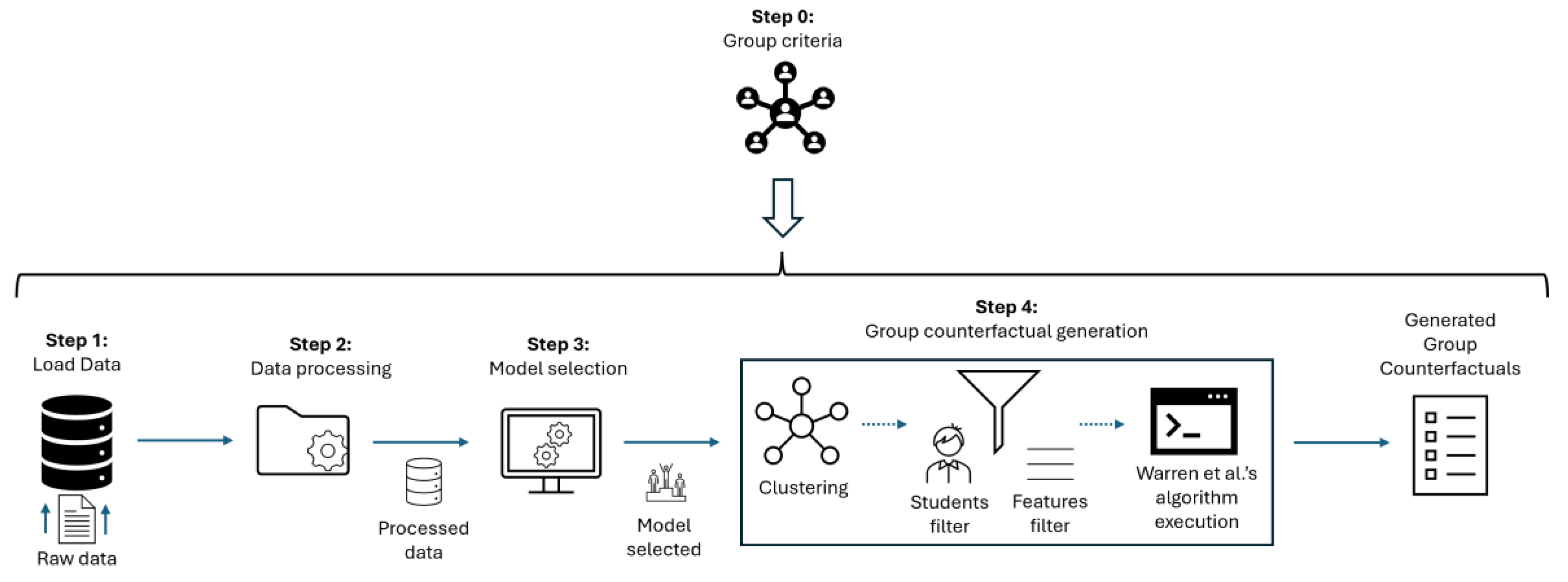
Figure 2.
Random Forest's confusion matrix.
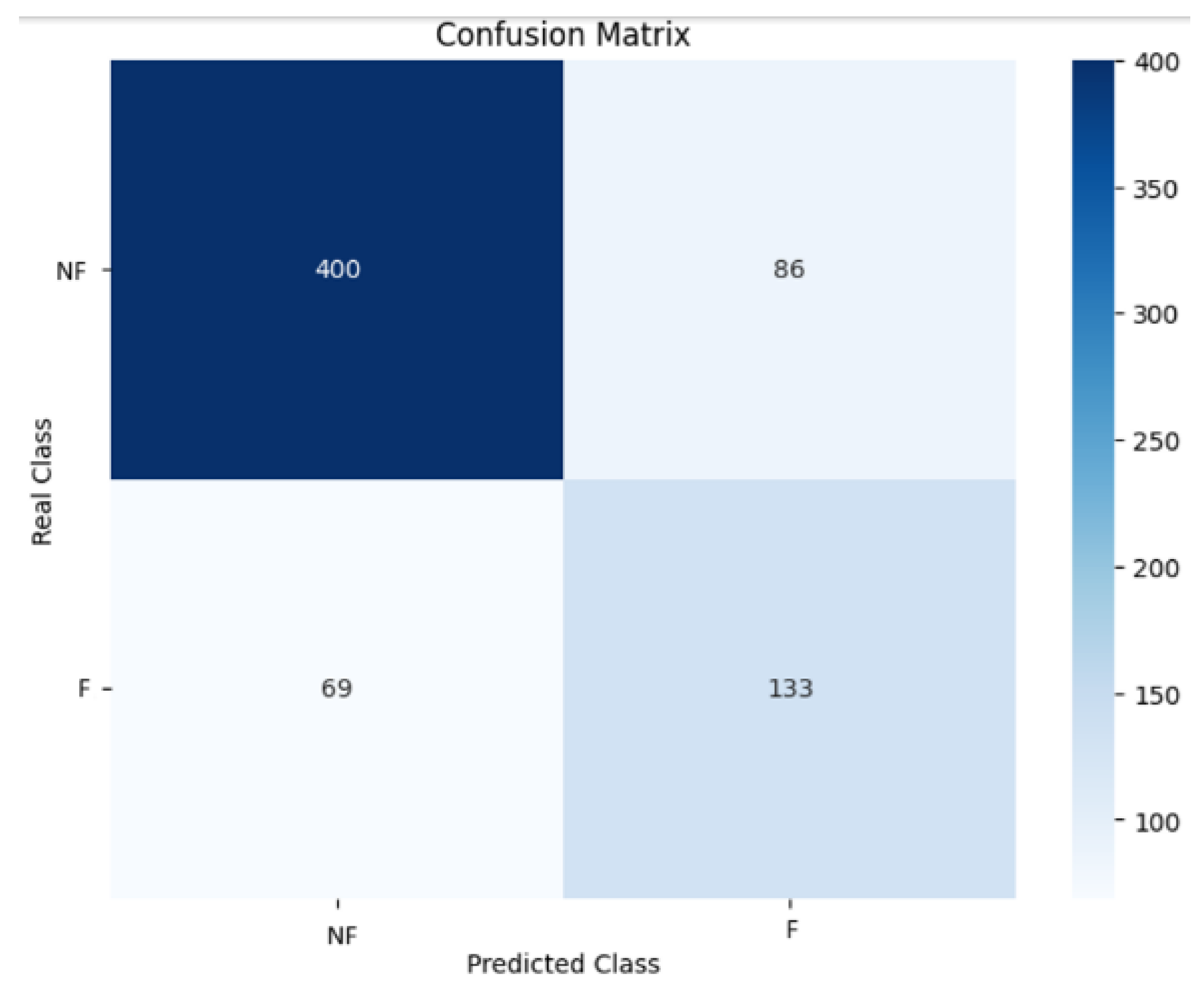
Figure 3.
AutoGluon's confusion matrix for ExtraTrees_r4_BAG_L1.
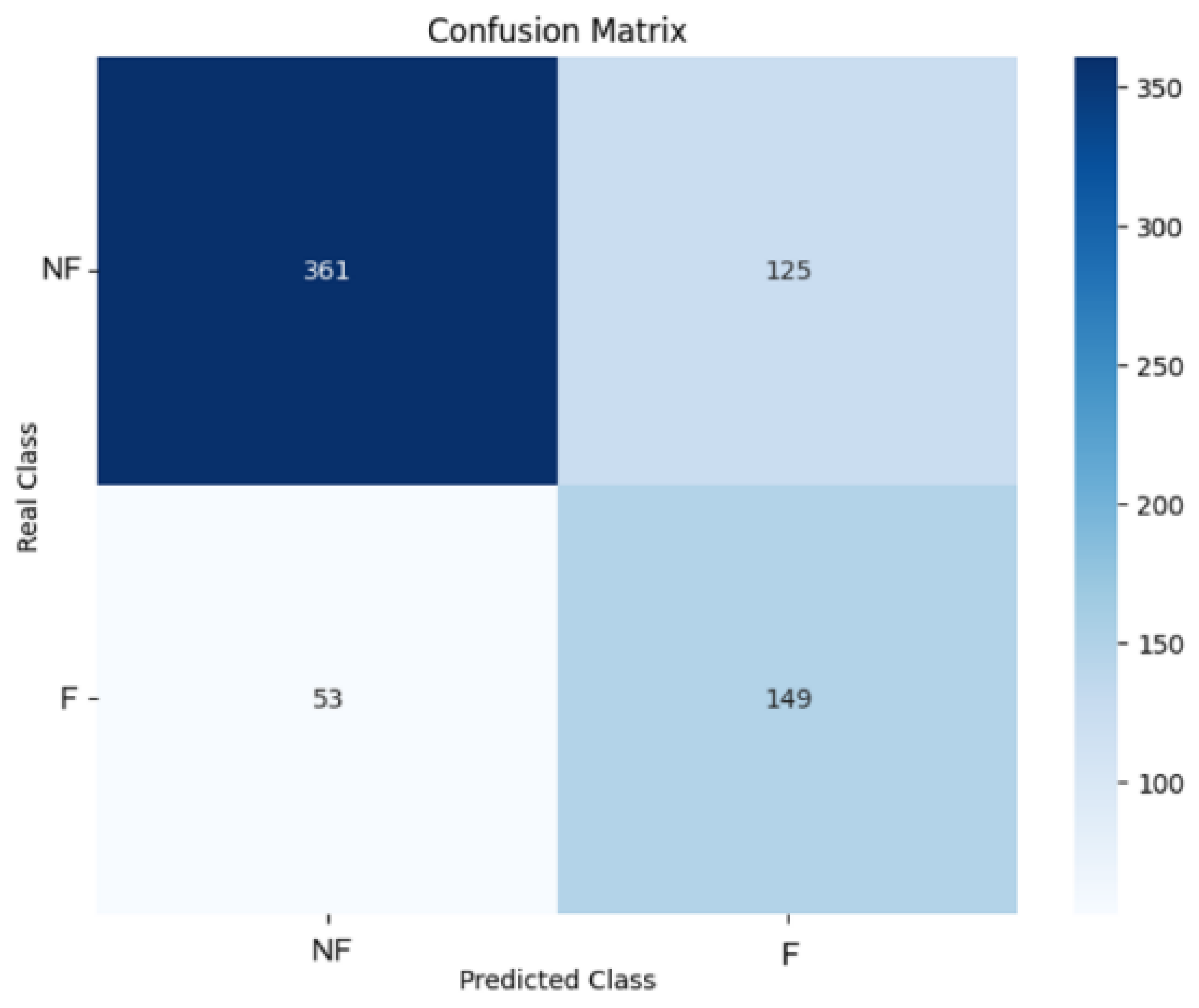
Figure 4.
Elbow method in our use case.
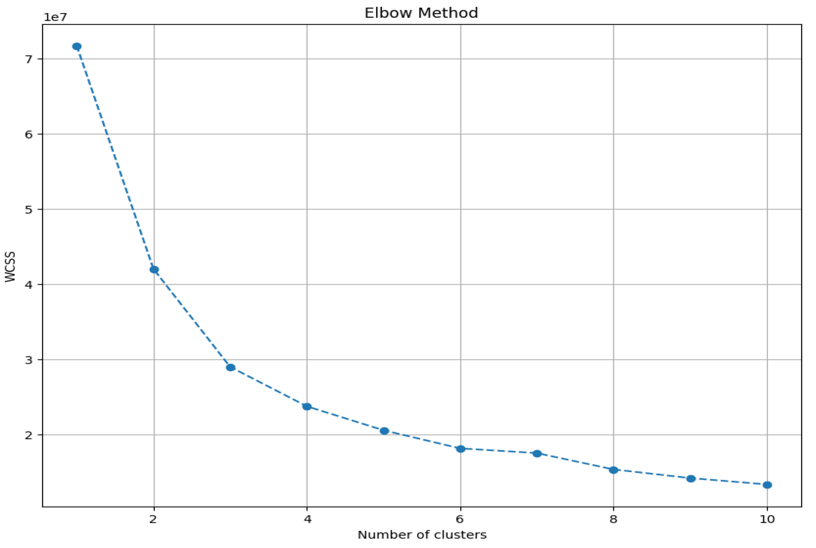
Figure 5.
Example of Greedy chart with group counterfactual for Cluster 0 made with CounterPlots library of Python.
Figure 5.
Example of Greedy chart with group counterfactual for Cluster 0 made with CounterPlots library of Python.
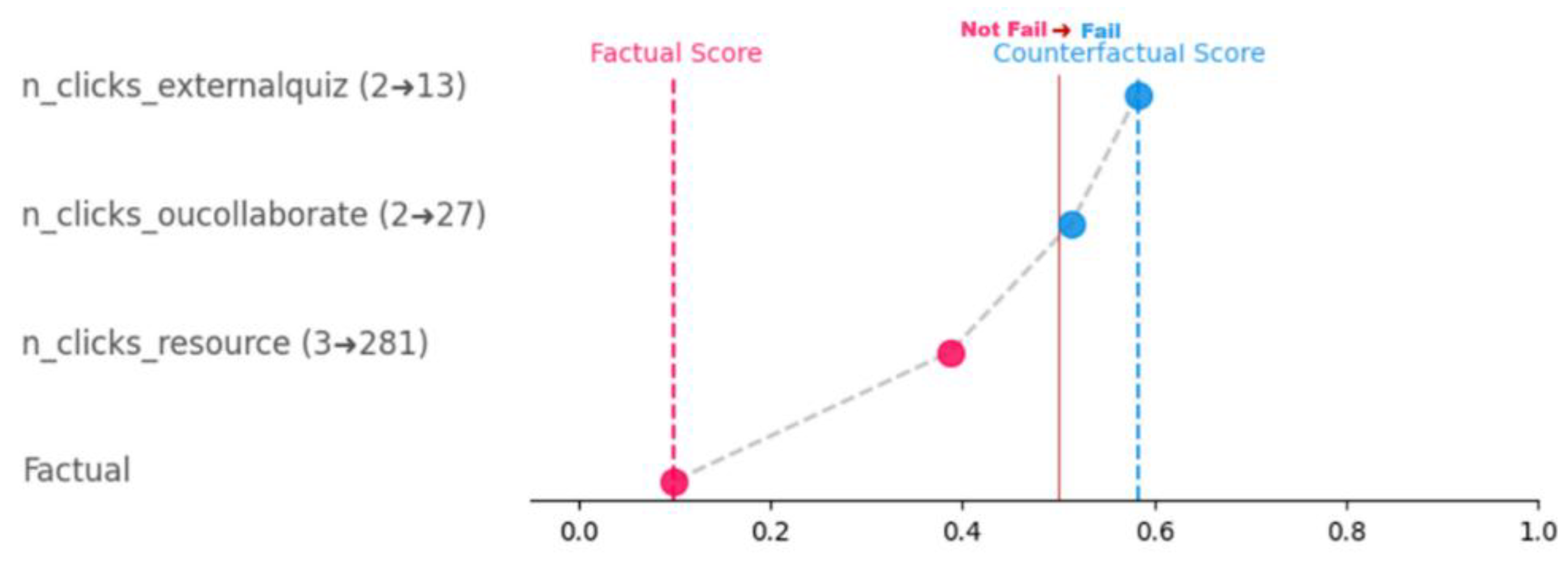
Table 1.
Autogluon best models.
| Models | F2-score |
|---|---|
| ExtraTrees_r4_BAG_L1 | 0.688 |
| RandomForest_r34_BAG_L1 | 0.683 |
| ExtraTrees_r172_BAG_L1 | 0.675 |
| ExtraTrees_r126_BAG_L1 | 0.668 |
| ExtraTrees_r178_BAG_L1 | 0.663 |
| RandomForest_r15_BAG_L1 | 0.649 |
| RandomForestGini_BAG_L1 | 0.645 |
| RandomForest_r166_BAG_L1 | 0.645 |
| RandomForest_r39_BAG_L1 | 0.642 |
| RandomForest_r127_BAG_L1 | 0.641 |
Table 2.
Cluster analysis.
| 0 | n_students | n_clicks_externalquiz | n_clicks_forumng | n_clicks_glossary | n_clicks_homepage | n_clicks_oucollaborate | n_clicks_oucontent | n_clicks_ouwiki | n_clicks_resource | n_clicks_subpage | n_clicks_url | |
|---|---|---|---|---|---|---|---|---|---|---|---|---|
| 0 | 499 | mean | 3.5 | 59.38 | 4.53 | 92.75 | 3.35 | 86.57 | 11.85 | 22.3 | 58.76 | 7.02 |
| stdev | 4.8 | 59.9 | 13.41 | 61.16 | 6.84 | 78.56 | 24 | 19.44 | 51.43 | 7.9 | ||
| 1 | 12 | mean | 20.91 | 1239.41 | 11.08 | 978.83 | 29.75 | 215.41 | 130.25 | 114.41 | 491.75 | 52.16 |
| stdev | 13.48 | 607.38 | 19.2 | 332.84 | 21.61 | 168.3 | 105.75 | 56.66 | 261.24 | 30.7 | ||
| 2 | 165 | mean | 10.02 | 302.52 | 8.66 | 293.34 | 13.67 | 186.01 | 59.81 | 70.97 | 217.37 | 29.6 |
| stdev | 10.24 | 164.73 | 36.57 | 112.15 | 17 | 131.97 | 60.56 | 62.9 | 130.58 | 28.42 |
Table 3.
Metrics for evaluating the obtained clusters.
| Name | Explanation | Value | Interpretation |
|---|---|---|---|
| Silhouette [45] | It takes values between -1 and 1, the closer to 1 the better. It evaluates the quality of the clusters by indicating how well each data point within its own cluster compares to other clusters. Values close to 1 indicate that the points in the cluster are similar to each other, while a value close to -1 indicates that the points are closer to a different cluster than the one that was initially assigned |
0.49 | This value indicates that the clusters are moderately well defined. While most points seem reasonably assigned to their clusters, some overlap between clusters is likely present |
| Davies-Bouldin [46] | It takes values greater than or equal to 0, the higher the better. It evaluates the quality of the clusters by focusing on the relationship between the distance within clusters (intra-cluster) and the distance between clusters (inter-cluster). A value close to 0 indicates a good separation between clusters, while high values would indicate an overlap between clusters |
0.65 | This suggests that the clusters have moderate internal dispersion and that the separation between clusters may not be very distinct, pointing to a less compact cluster structure |
| Calinski-Harabasz [47] | It takes values greater than or equal to 0, the higher the better. It evaluates the quality of clusters based on the ratio of intra-cluster dispersion to inter-cluster dispersion. A high value indicates better defined clusters, where the points within each cluster are more grouped and the clusters are well separated from each other, while a lower value suggests worse quality, with high intra-cluster dispersion | 494.16 | This score suggests that the clusters exhibit moderate cohesion and separation. A higher score typically indicates better-defined clusters, while this value points to a somewhat looser cluster formation. |
Table 4.
Group counterfactuals generated.
| Cluster | n_clicks_externalquiz | n_clicks_forumng | n_clicks_glossary | n_clicks_homepage | n_clicks_oucollaborate | n_clicks_oucontent | n_clicks_ouwiki | n_clicks_resource | n_clicks_subpage | n_clicks_url |
|---|---|---|---|---|---|---|---|---|---|---|
| 0 | 13 | - | - | - | 27 | - | - | 281 | - | - |
| 1 | 17 | 788 | - | - | 25 | - | - | - | - | - |
| 2 | - | - | 182 | 498 | - | - | - | 76 | - | - |
Table 5.
Results obtained with different % features (average values considering all clusters).
| % features | Validity | Execution time |
|---|---|---|
| 10 | 0.953 | 232.24 |
| 20 | 0.963 | 32.39 |
| 30 | 0.993 | 30.33 |
| 40 | 0.993 | 19.86 |
| 50 | 0.996 | 28.01 |
Table 6.
Results obtained with different students’ selection approaches and different % students (average values considering all clusters and the 30 runs).
Table 6.
Results obtained with different students’ selection approaches and different % students (average values considering all clusters and the 30 runs).
| Technique | % students | Validity | Average time (s) |
|---|---|---|---|
| Closest | 1.0% | 0.969 | 4.37 |
| 5.0% | 0.966 | 18.3 | |
| 10.0% | 0.962 | 35.35 | |
| 15.0% | 0.922 | 22.67 | |
| 20.0% | 0.986 | 44.43 | |
| 25.0% | 0.993 | 92.13 | |
| 50.0% | 1.0 | 192.8 | |
| Farthest | 1.0% | 0.959 | 7.91 |
| 5.0% | 0.963 | 36.05 | |
| 10.0% | 0.957 | 58.64 | |
| 15.0% | 0.990 | 34.54 | |
| 20.0% | 0.980 | 44.22 | |
| 25.0% | 0.999 | 112.18 | |
| 50.0% | 1.0 | 204.17 | |
| Random | 1.0% | 0.937 | 4.51 |
| 5.0% | 0.967 | 38.05 | |
| 10.0% | 0.987 | 42.49 | |
| 15.0% | 0.977 | 32.86 | |
| 20.0% | 0.984 | 44.54 | |
| 25.0% | 1.0 | 117.32 | |
| 50.0% | 1.0 | 189.27 | |
| Full | 100.0% | 1.0 | 364.18 |
Table 7.
Comparative of group and individual counterfactuals (average values considering all the instances in each cluster for each type of counterfactual – individual or group).
Table 7.
Comparative of group and individual counterfactuals (average values considering all the instances in each cluster for each type of counterfactual – individual or group).
| Cluster | Cluster students | Counterfactual type | Validity | Sparsity | Proximity | Execution time (s) |
|---|---|---|---|---|---|---|
| 0 | 499 | Individual | 1.0 | 0.816 | -21.93 | 239.50 |
| Group | 1.0 | 0.7 | -10.748 | 62.94 | ||
| 1 | 12 | Individual | 1.0 | 0.848 | -9.814 | 5.77 |
| Group | 1.0 | 0.7 | -0.914 | 1.58 | ||
| 2 | 165 | Individual | 1.0 | 0.848 | -5.835 | 79.85 |
| Group | 0.98 | 0.7 | -0.781 | 26.46 |
Disclaimer/Publisher’s Note: The statements, opinions and data contained in all publications are solely those of the individual author(s) and contributor(s) and not of MDPI and/or the editor(s). MDPI and/or the editor(s) disclaim responsibility for any injury to people or property resulting from any ideas, methods, instructions or products referred to in the content. |
© 2025 by the authors. Licensee MDPI, Basel, Switzerland. This article is an open access article distributed under the terms and conditions of the Creative Commons Attribution (CC BY) license (http://creativecommons.org/licenses/by/4.0/).
Copyright: This open access article is published under a Creative Commons CC BY 4.0 license, which permit the free download, distribution, and reuse, provided that the author and preprint are cited in any reuse.


