1. Introduction
Automated artificially intelligent systems are increasingly intertwined with our everyday lives — from medical diagnosis to finance and image recognition. While some situations will use directly interpretable models — such as logistic regression [
1] — others will be black-box [
2]. For consumers to trust these black-box models, they often want some explanation as to what this automated system is doing — an answer to why it made the decision it did. Explainable AI (XAI) is a field of research that aims to develop tools and techniques to answer these questions. Many existing tools exist for generating these explanations for end users. Popular tools include SHAP [
3] and LIME [
4] XAI can also be used for debugging models by finding where the model has learnt spurious relationships in the training data and providing algorithmic accountability. Some proposed legislative frameworks have begun to demand this accountability from applied algorithms [
5].
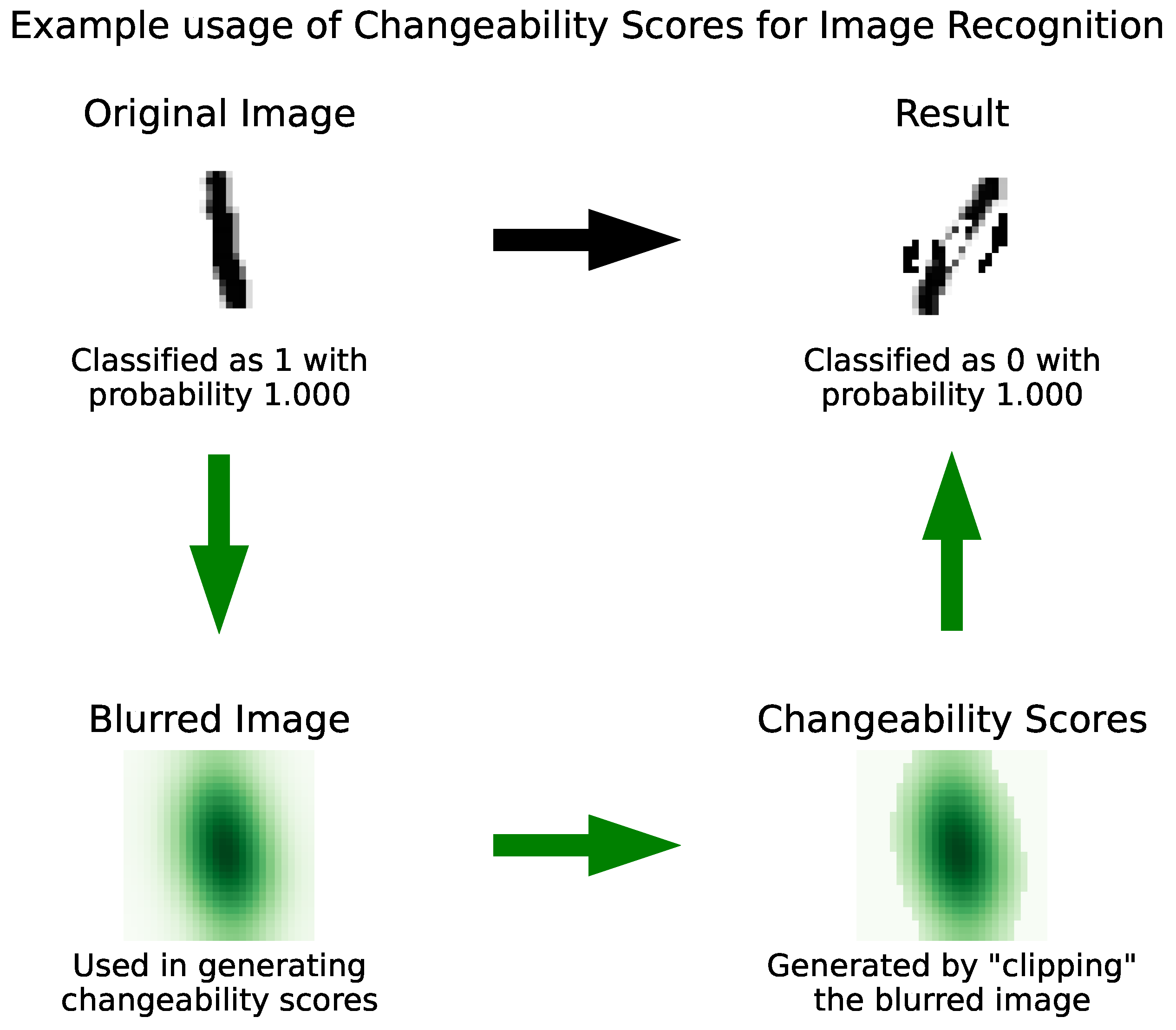
One way to provide these explanations is through counterfactuals. The classic example of a counterfactual explanation of a model involves a situation where we have trained a model to decide whether a bank should provide an individual with a loan. A helpful way to explain the predictions this model makes is to say what a user must modify to change the prediction made by a model. For example, “You were denied this loan, but if your income was £10,000 higher, you would have been granted this loan”, or “You were granted this loan, but you would not have been granted a loan of a higher value”. Similarly, we could say “This image was classified as a 1, but if we filled in these pixels, the image would be classified as a 0.” This way of explaining the output of machine learning models has a number of benefits over existing models. In some sense, it is actionable to a user. Similarly, they may be easier to interpret - as this is an intuitive form of explanation that users will have encountered in their day-to-day lives.
Formally, given a data point x and a classification model f, we define a counterfactual as a different data point such that . We want our counterfactual point to be, by some metric, close to the original point.
As with some existing research in this field [
6], we aim to bring together ideas from program synthesis and explainable AI to develop a methodology for generating counterfactuals to explain the outputs of black-box systems. We chain together a series of individual changes. The selection of changes, which are themselves determined by local, simple surrogate models, are easily fine-tunable by an end user.
Overall, according to some quantitative and qualitative metrics, our novel methodology performs better than certain common existing methodologies on some data formats. Furthermore, our method can provide insights into how the model processes information, especially in the case of images.
1.1. Our Approach
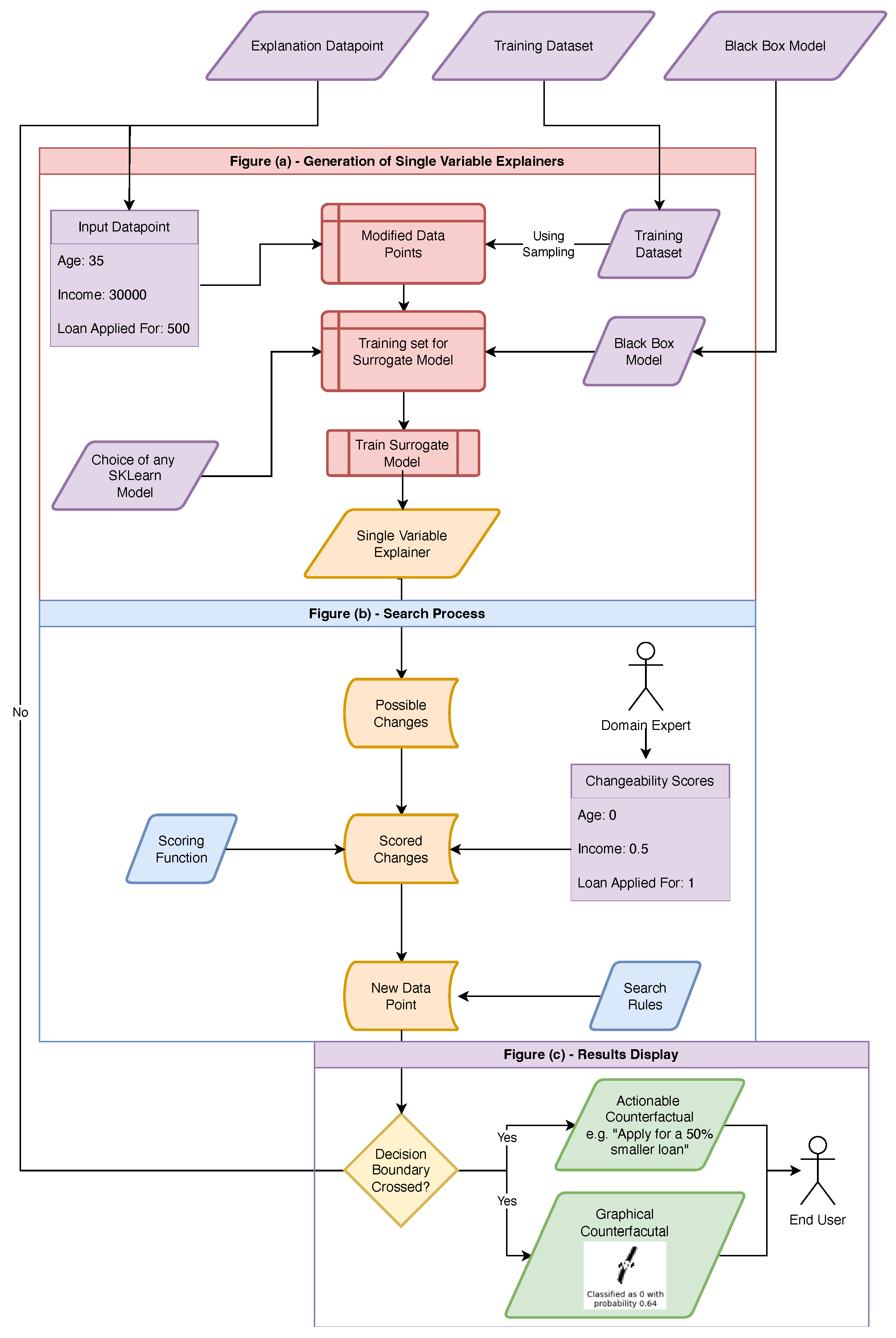
We develop an approach that can produce counterfactual explanations (see
Figure 1). We begin by varying the value of each input feature to generate hypothetical fake data-points. Once we have these we are able to apply our original model to this new local data-set (
for our underlying model
f) .
We then fit surrogate models (such as a Gaussian process) to the effect of varying each feature. These surrogate models estimate the high-level, local dependence of the underlying model on each feature. If any of these models predict that a possible feature value change is, in fact, a counterfactual , we stop here - returning this to the end user. If not, we “score” each of these single variable explainer, and repeat the process from these new, fake data points.
This scoring phase allows for a domain expert to tune the explanation, through setting “changeability scores” for different variables, or by customising the scoring function itself.
2. Background
Automated systems driven by artificial intelligence are becoming integrated into our lives – from medical diagnoses to financial services and image analysis. While some employ interpretable models, such as logistic regression [
1], others utilize black-box models [
2]. To gain consumer trust in these black-box models, it is often necessary to provide some explanation of the system’s operations – essentially, why a particular decision was reached.
Explainable AI (XAI) is focused on creating tools and methodologies to address these questions. XAI can also aid in model debugging by identifying where the model has learned incorrect patterns from the training data and ensuring algorithmic accountability. AI models are very effective at solving a wide range of problems [
7], they are often a black box [
2] – i.e., characterised by their inputs and outputs but whose inner workings cannot be directly interpreted by a user or programmer.
Due to the growing popularity of AI in high-stakes decision-making [
8], there has been a vast body of research into techniques to explain the decisions of these models [
9]. Some state-of-the-art techniques include feature attribution models such as SHAP [
10] and LIME [
4]. Other methods rely on gradients – such as GRAD-CAM [
11], or concept-based explainability, such as through concept bottleneck models [
12] – often with automated concept extraction [
13,
14].
We use some ideas from the LIME paper – such as fitting simple surrogate models to perturbations around our sample of interest - alongside ideas from the SHAP paper - such as working on a feature-by-feature basis.
2.1. Counterfactuals
One way to provide these explanations is through counterfactuals [
15]. The classic example of a counterfactual explanation of a model involves a situation where we have trained a model to decide whether a bank should provide an individual with a loan. A helpful way to explain the predictions this model makes is to say what a user must modify to change the prediction made by a model. For example, “You were denied this loan, but if your income was £10,000 higher, you would have been granted this loan”, or “You were granted this loan, but you would not have been granted a loan of a higher value”. Similarly, we could say “This image was classified as a 1, but if we filled in these pixels, the image would be classified as a 0.”
Formally, given a data point x and a classification model f, we define a counterfactual as a different data point such that .
The problem of finding counterfactuals (sometimes referred to as the inverse classification problem [
16]) is an active area of research. In the next section, we will review some of these methods; however, this is not meant to be an exhaustive review, but instead just to give an overview of the range of existing methods.
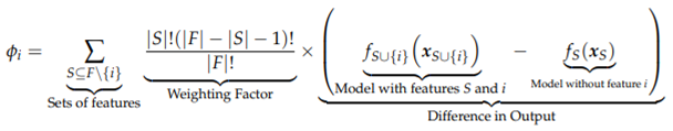
2.2. SHAP Values
[
10] introduce a technique for assigning importance to different features by (using ideas from game theory) taking the difference between models trained with and without the feature present.
However, this computation is incredibly expensive, but for most models, we can approximate this using Monte Carlo methods.
The authors also developed a Python library [
3] implementing this.
2.3. LIME
Local Interpretable Model-agnostic Explanations (LIME), introduced by [
4], works by fitting simple, explainable models to the local behaviour of the model. They choose the explainer model
as follows:
Where
measures how unfaithful
g is in approximating
f in the locality defined by
,
G is the class of simple models being considered and
guides towards simpler explainer models. In effect, this finds the best simple, interpretable model in the neighbourhood of the relevant point and uses this to explain the model’s decisions. They focus on the case where
G is the class of linear models and use the locally weighted square loss as
. They show that this works well for text and image classification.
2.3.1. Existing Methodologies for Generating Counterfactuals
[
17] is considered one of the first papers to introduce counterfactuals [
18]. They treat this as an optimisation problem on the loss function
for some distance function
d. Researchers can use various strategies to complete the optimisation – some of which, such as Adam [
19], require gradient-level access to the model, whereas others, such as Nelder-Mead [
20], do not.
[
18,
21] perform large-scale reviews of the existing research on finding counterfactuals. Guidotti begins by highlighting several beneficial properties – such as validity (that it is genuinely counterfactual), similarity (that the distance between the original data point and the counterfactual data point is sufficiently small), actionability and others that we do not have space to list in this report.
Model Specific Explanations
While many proposed methods are model-agnostic, others are designed to work with specific models. For example, [
22,
23,
24] focus on tree-based models, [
25,
26] focus on Linear Classifiers. Similarly, [
27] focus on Random Forests [
28] while [
29] focus on Boosted Trees [
30,
31].
Counterfactuals as an Optimisation Problem
Generally, the problem of finding counterfactuals can be considered an optimisation problem [
21]. Various researchers investigate different algorithms for solving this optimisation problem — for example, [
32] utilise a “Growing Spheres” algorithm, while [
33,
34] utilise FISTA (Fast Iterative Shrinkage-Thresholding Algorithm) [
35]. Other researchers, such as [
36], fit simpler, interpretable models to the output of the more complex model within a neighbourhood of the data point. We build on this by fitting simpler models to the effect of varying each feature.
Similarly, [
37] treat this as a “Multi-Objective” Optimisation problem – including distance from the original point, number of changed features and how well the counterfactual point fits the original distribution. Using the multi-objective optimisation framework, they return a “Pareto set” of counterfactuals representing different trade-offs between their proposed objectives. [
38] expand on this by also including a “causality” objective.
Van Looveren et al. [
39] improve on optimisation-based strategies by using Auto-encoders [
40] to build “Class Prototypes” and including this as a term in the optimisation problem. Similarly, [
41] use the Mahalanobis’ distance [
42] and the local outlier factor [
43] to create distribution-aware counterfactuals. Additionally, [
44] expand on such strategies by building in causal constraints, while [
45] use variational auto-Encoders [
46].
Sequential Counterfactuals
Sequential counterfactuals differ from traditional counterfactuals in the sense that they provide not just examples of nearby points that have the opposite classification but that they also provide a sequence of steps. [
21] note that sequential counterfactuals are an active area of research. [
47] demonstrate, through a user study, that end-users generally strongly prefer such directive explanations. However, they note that social factors can affect these preferences.
Similar Work
Similar to our proposal, [
6] chain together instances of possible changes to find counterfactuals. In their proposed methodology, a domain expert would curate a list of plausible changes and Boolean pre-conditions for when these changes could be made. An optimisation algorithm using the model’s gradient is then used to find the best (by some scoring metric) counterfactual for that instance. A range of papers build on this work. For example, [
48] expand on this, allowing it to work on non-differentiable models, provide multiple solutions, and improve efficiency through pruning. They also build on the Boolean pre-condition model of when changes can be made by introducing a notion of consequences (e.g. age increases as a consequence of obtaining a higher degree).
Our project differs from existing research in a few critical aspects. Firstly, both Ramakrishnan et al.’s [
6] and Naumann & Ntoutsi’s [
48] methodologies use a pre-defined series of actions that can be taken. This approach has numerous advantages; it can model the relations between different variables well – for example, in a financial application, doubling the income would also reduce the debt-to-income ratio. However, this would require a significant time investment for a domain expert to collate. Our approach (explained in the next section), through fitting simple surrogate models, can choose the most effective changes to make without this. We design our scoring mechanism to be easily interpreted by a domain expert – meaning results can be efficiently personalised.
2.3.2. Other Methodologies We Evaluate Our Methodology Against
To examine the effectiveness and utility of our novel methodology, we compare it with some existing methodologies to generate counterfactuals. We chose these options as there are publicly available Python packages [
49,
50] implementing these. As we also make a Python implementation of our methodology publicly available [
51], these are reasonable points of comparison — although it is not exhaustive.
AlibiExplain, developed by Klaise et al. [
50] implements the method described by Wachter et al. [
17]. This methodology works by performing the following minimization, where
is the counterfactual data-point:
In this case,
represents the point we are trying to find a counterfactual for,
is the model and
d is some distance metric. Wachter et al. propose using the ADAM distance metric [
19].
Klaise et al. also implement a more complex methodology that utilizes prototypes, as introduced by Van Looveren et al. [
52]. This methodology also minimizes a loss function
over some
D-dimensional feature space. The loss function they use is
encourages the class to change,
penalizes (by a factor of
) out of distribution counterfactual instances (by using the
reconstruction error from an auto-encoder and,
acts by a factor of
to both speed up the search process and guide the perturbation towards an interpretable counterfactual, and
and
correspond to the usual norms.
2.3.3. Practical Uses of Counterfactual Explanations
As with all forms of explanation for automated systems, they can increase a user’s trust in an automated system [
53]. By attempting to approximate the reasoning that these automated systems have employed, users can assess whether they agree with this reasoning. These counterfactual explanations can also be tuned to be actionable — this means that an end-user can take actions based on their received explanations. For example, if an explainer suggests that an applicant was denied for a loan but would have been accepted for a smaller loan, the applicant can respond by applying for this smaller loan. Similarly, in a medical situation, if the explainer suggests that a patient who exercised more would be less likely to have severe complications from a disease, the patient could respond by doing this. Of course, not all changes are possible for all situations, so a tuneable, human-in-the-loop methodology is beneficial.
Similarly, users of an automated system are entitled to an explanation of why such a system made the decision it did [
54]. Counterfactual explanations can be one part of meeting this legal requirement [
55]. Counterfactuals can also help data scientists understand the model’s internal structure better and correct for unintentional biases in the training data. For example, suppose that counterfactuals generated for a financial model suggest that “protected characteristics” should be changed to change the output of the model. In that case, it is likely that the model has learnt unintended biases and that further work is needed to de-bias the training data before deploying the model in practice.
When domain experts are presented with such counterintuitive explanations, they can be prompted to examine the training data set for these biases, leading to fairer, more accurate models. Ultimately, this also can be a part of legal requirements to conduct impact assessments for model bias and effectiveness [
5].
2.4. Relation to Adversarial Machine Learning
Adversarial Machine Learning is closely related to Counterfactual Explanations. As discussed by [
56], many families of machine learning models are vulnerable to adversarial examples: inputs specifically designed to cause the target model to produce erroneous outputs. This problem of modifying an input to “trick” the model into giving a different output is, at a high level, similar to that of finding counterfactuals. While there is a difference in focus - instead of trying to trick the model, counterfactual explanations focus on providing useful explanations to users - this similarity has been exploited to develop strategies for generating counterfactuals, for example, by [
52]. Similarly, [
57] utilise Generative Adversarial Networks [
58].
3. Methods
3.1. Methodology for Generating Counterfactuals
We can summarize our general methodology as follows:
-
Fit simple, surrogate models to the effect of changing each input feature in the underling model, keeping all other features the same.
We might for example, fit linear models to the local effect of changing each pixel of an image, or the effect of each input feature to a system that makes decisions about whether applicants are entitled to loans.
Consider the example where we have an individual with an income of £30k, applying for a loan of £1k. We will imagine this individual has a debt-to-income ratio of 10% and they are denied a loan by the hypothetical system (with a class probability of 0.9).
-
For each of these models,
- (a)
-
Select the `feature value’ that they predict will maximise the “score”.
- (b)
-
In the initial data-point, replace this feature with this new value.
-
If any of these new data-points change the model prediction (possibly plus some additional threshold), this is the counterfactual.
Suppose running this original classifier now accepted the applicant the loan, with a class probability of 0.6. We can take this new data-point as counterfactual and return it, in a human-readable-format to the user.
-
Otherwise, select the best scoring one of these new data-points and repeat the process from here.
If instead, the system still denied the use the loan, but this time with a class probability of 0.6, we take this new hypothetical point and repeat the process from here.
Note: we would in fact do this for all allowed input data-points and pick the one which maximised some score.
-
If we have run out of variables to change - or reached the maximum search depth - then return to previous unexplored branches and search from there.
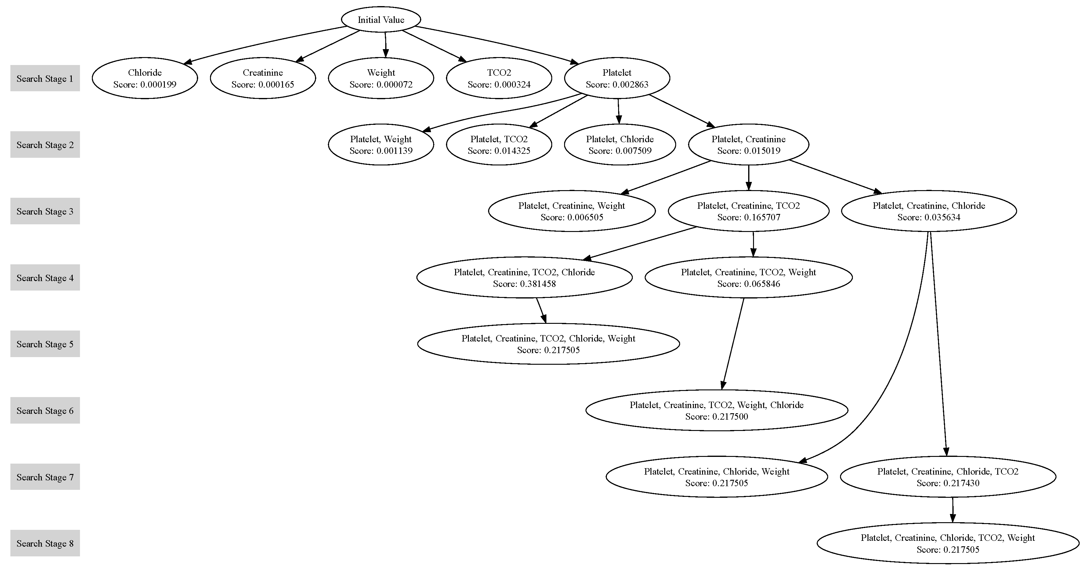
We can think of the change to single variable as being a node on a graph, connected to points it shares “all but one feature value” with. In this sense, our search process is akin to a depth-first-search on this graph. This is visualised in
Figure 3
Repeat the previous step until either a counterfactual has been found, or all notes of the graph have been searched.
We note that we have built our system such that it is modular, so that we can easily change the search process. For example, we can change the order in which we change the features. We can also change the stopping criteria — i.e. when we stop changing features and decide there does not exist a counterfactual subject to the given criteria.
By some metrics, our method can be considered to be generating local counterfactuals. Since it starts from the initial data-point and aims to make small changes until it shifts the model’s prediction, it inherently tries to make as few changes as possible. However, through our tunable changeability scores and scoring functions we made it possibly to change how “local” these counterfactuals truly are.
3.1.1. Surrogate Models
These surrogate models, which we will often refer to as single variable explainers (SVEs), attempt to explain the dependence of the model’s output on the variation of one parameter locally.
For a particular variable, we generate a set of input data points by replacing that variable with other values that the variable takes in the training data set. Either we do this through Monte-Carlo like sampling — i.e. replacing with randomly chosen other values in the data set — or by selecting uniformly placed points across some interval, such as (where is the variable’s mean value in the training data and is the standard deviation) or defined quantiles of the values of that feature in the training data. We then apply the (black-box) model to these to get a series of sampling variables and class probabilities pairs.
We then fit a simple explainable model to this new data set. We use either a Gaussian process or a linear model.
Our framework is sufficiently general to allow for any SciKit-Learn [
59] regression model to be used. The existing tools built in Keras [
60] also make our tool compatible with TensorFlow/Keras models. We discuss our technical implementation in more detail in
Section 3.2.
3.1.2. Scoring Rules
A range of rules can be used to score these models; by default, we consider the following, where
represents the score when the feature is changed from its original value to a new value
x.
This, measures the change in class probability caused by a given change in an input feature.
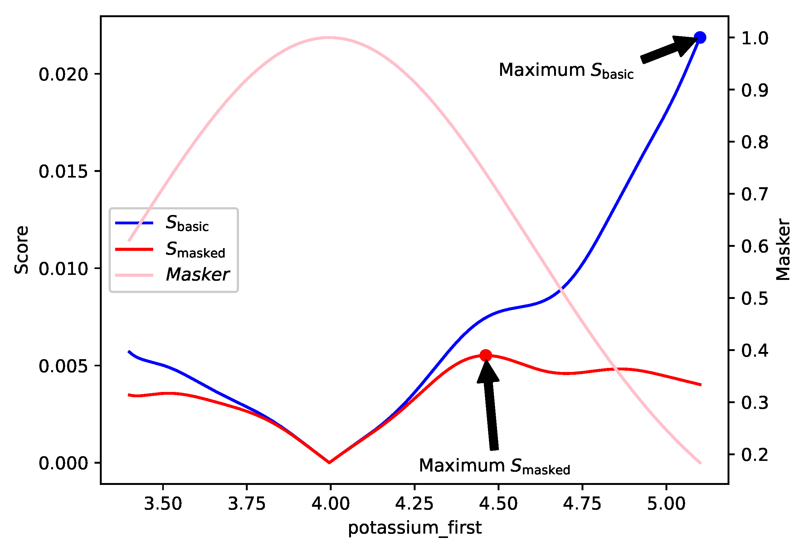
There may be situations, where there is a “cost“ to changing a feature too much, so we implement a “scorer” that allows for smaller changes. To encourage smaller feature changes we can apply the following mask:
Finally, each score is weighted by a user-provided “feature changeability score” that quantifies the ease with which a feature can be changed. .
Borrowing ideas from the field of human-computer interaction, this allows the user to tune the methodology to their use case. This is visualized in
Figure 2.
As mentioned above, a user could choose a “masked” scoring function with a small standard deviation to guide the methodology for selecting small changes.
3.1.3. Benefits
There are several benefits to counterfactuals as a method for explaining the output of machine learning models. Indeed, through a user study, [
61] demonstrate, that counterfactual explanations elicit greater satisfaction and trust than causal explanations.
Similarly, these counterfactual explanations can be considered more actionable to an end user - especially sequential counterfactuals, which can act as a series of steps for a user to take. This is confirmed by [
47].
Our method also has a number of specific benefits. Firstly, it’s modularity makes it easy to specialise to specific situations. We explain how we achieved this modular structure in our “Technical Implementation" section. Similarity, our “scorer“ builds in ideas of a “changability score” which makes our method tunable by a domain expert or end user.
Figure 3.
This figures shows our search process. Here, we used our method to explain the output of a medical model. Each node represents a single variable explainer trained on the specified feature around the maximum scoring data point of the node’s parent. Each layer of the graph represents a set of single variable explainers that are evaluated together. This graph demonstrates the depth first nature of our process.
3.2. Technical Implementation
We have made our tool open-source and available on GitHub, with full documentation included in this repository.
We also make it available as a python package for easy installation.
pip install tuneable-counterfactuals-explainer
Our method, implemented in Python, can wrap around any black-box model with a
predict_proba method that can take in a Pandas [
62] DataFrame and return a list of tuples of class probabilities. This is the case for SciKit-Learn [
59] models.
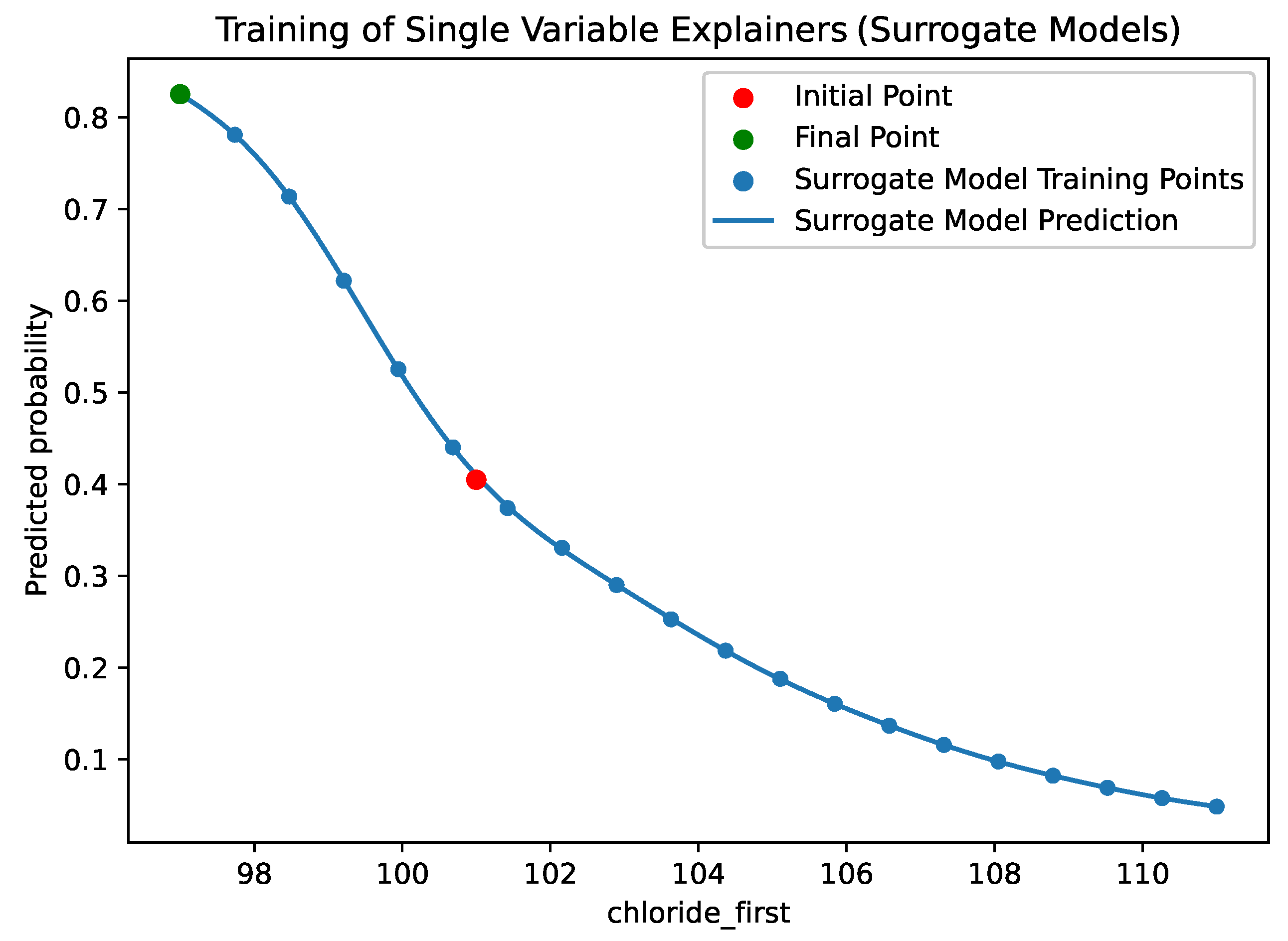
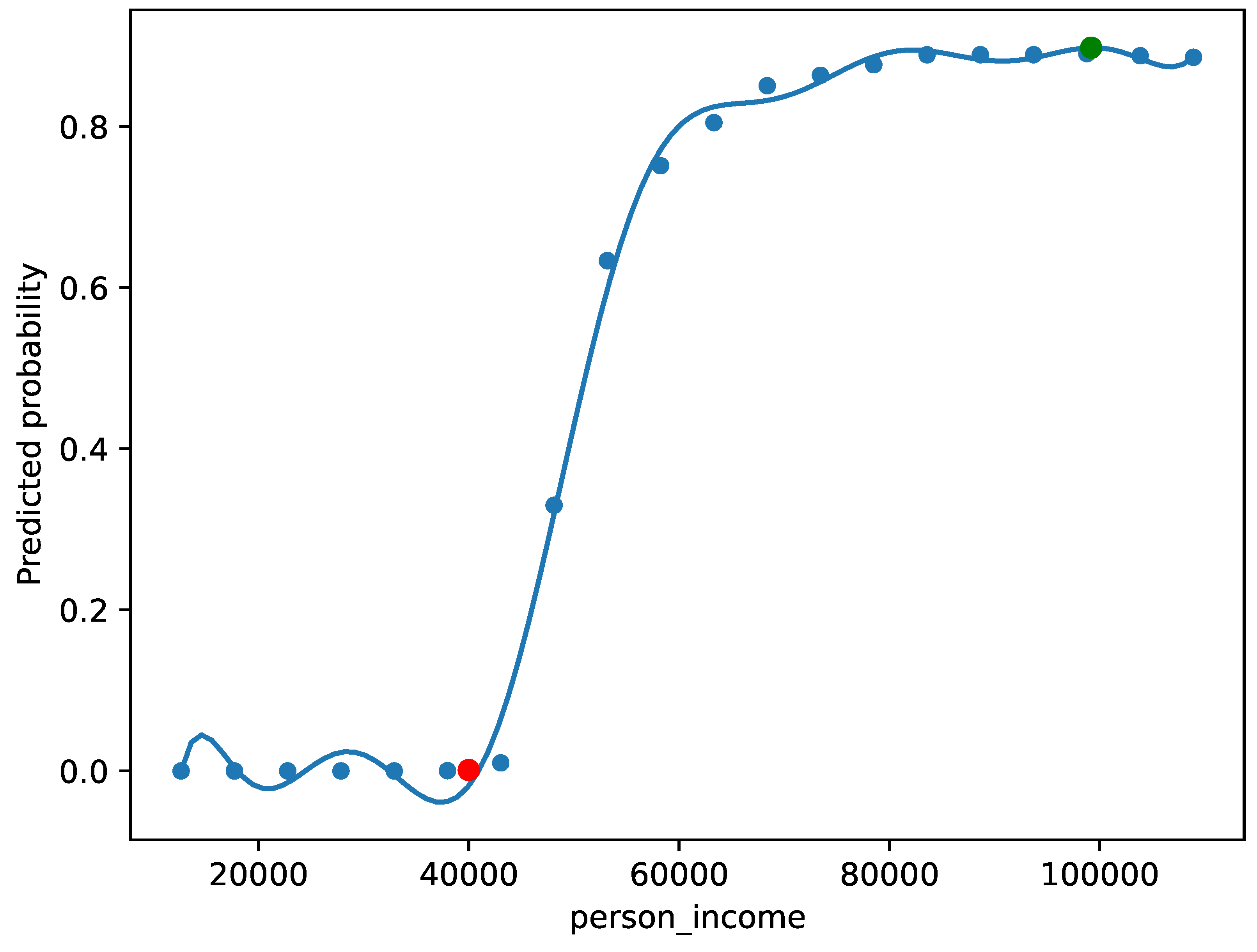
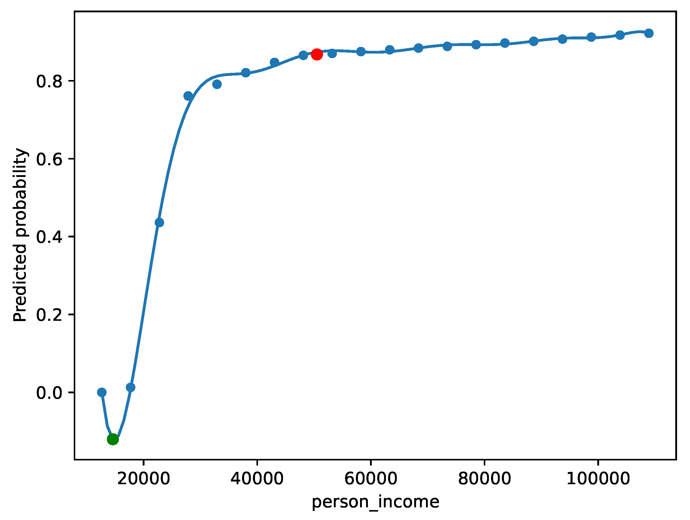
Figure 4.
This graph shows the process of training the “SingleVariableExplainer” objects. The red point shows the initial value of the chloride_first feature against the initial class probability for the classification. The blue points represent hypothetical new patients, with a changed chloride_first value (initial amount of chloride measured at admission time), but with all other features remaining the same. We plotted the new feature values against the class probability for these new hypothetical patients. It can be seen that we have used uniform sampling for these points. The blue line represents the Single Variable Explainer (SVE) itself, in this case a Gaussian Process surrogate model. The green point, represents the selected best change to the feature, according to the scoring function.
Our method is implemented as a “explainer object”, into which a end-user passes a model to be explained, the data used to train the model and the target variable of the model. This object, with an “explain” method calls a “searcher” object which generates “single variable explainer” objects. These are scored by “scorer” object. “Sub-classes” can be created for any of these objects to specalise the method for a given situation. The user can also specify additional optional parameters that guide the counterfactual process as outlined in
Table 1.
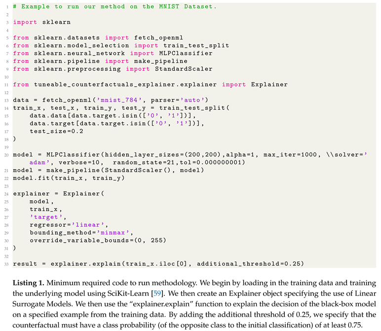
We include an example of the code required to run our method in Listing 1.
3.3. Evaluation Methodology
We evaluate our method by training simple models on simple data-sets and evaluating how the counterfactuals generated by our model compare to those generated by some existing methodologies for generating counterfactuals. While this is not an exhaustive comparison, we have chosen some methodologies with existing publicly available implementations as valuable points of comparison. As our framework is available as an easily installable Python package, this accurately compares what other options domain experts will have at their disposal to explain machine learning models. We will use qualitative and quantitative metrics to evaluate our counterfactuals compared to those generated by other models.
3.3.1. Evaluation Metrics
We examine several quantitative metrics to analyse the performance of our algorithm.
An ideal algorithm to generate counterfactuals will be able to generate them quickly. However, since the performance of our algorithm is highly dependent on the hardware used, we do not include a speed evaluation of our method.
Additionally, as we want our counterfactual to be close to the original data point, we compare the distance to the original data point in terms of both the and norms.
Similarly, we want our counterfactuals to change as few features as possible, so we also compare the number of feature changes. Furthermore, we often want our counterfactual to be plausible — coming from a distribution similar to the original training data set — so we shall also measure the standardized distance to the nearest training data point.
Some of our qualitative metrics will include those used by [
63]. We want our counterfactuals to be both unambiguous and realistic. However, we also want them to reflect the model accurately. We also qualitatively examine what we learn about the model from the counterfactuals, and how useful such a counterfactual may be to a user.
3.3.2. Evaluation Data-Sets
As we discussed in
Section 2.3.3, these counterfactual explanations can be useful in financial and medical situations, so we evaluate our methodology on these. Since our methodology can be easily visualized on image datasets, we also evaluate it on this.
Financial Data-Set
Our first evaluation uses a simulated data set [
64]
1. We made this decision due to the lack of publicly available data sets for which appropriate documentation of their data collection methods exists. Since this project aims to evaluate the methodology for explaining models rather than the models themselves, it is unlikely that using a simulated data set will significantly affect our results. This dataset will allow us to evaluate the causal explanations that our methodology can generate.
This data set contains 12 features (Age, Annual Income, Home-ownership, Employment length (in years), Loan intent, Loan grade, Loan amount, Interest rate, Loan status, Percent income, Historical default and Credit history length) and 32581 examples. It should be noted that we dropped the “loan_intent” column and reversed the “loan_status” column such that 0 indicates a default. This allowed us to use this as a proxy for whether the individual should receive the loan. Similarly, we converted all remaining categorical columns into numerical columns. An example processed loan applicant is included in
Table 2
This data set contains only a small amount of missing data: 3116 loans were missing interest rate data, and 895 were missing employment rate information. For this reason, we chose to remove these 3943 data points.
This dataset represents a realistic, practical example of the use of counterfactuals. Applicants for loans can be given realistic, actionable, advice for how to increase their likelihood of being accepted for a loan.
MIMIC
The MIMIC (Multi-parameter Intelligent Monitoring in Intensive Care) II data set [
65] contains physiological signals and vital signs time series captured from patient monitors, along with comprehensive clinical data for tens of thousands of Intensive Care Unit (ICU) patients. We use a smaller pre-processed version of this data set produced by [
66], which contains information about the patient, such as age, gender, weight, BMI, information as to if and when the patient entered ICU, information about the patient’s clinical and medical history.
MNIST
MNIST [
67] is a large data set of labelled handwritten digits. It contains 70000 individually labelled 28 by 28 images with pixel values being integers from 0 to 255. This handwritten digit data set is standard across research in this field [
21], presenting a valuable point of comparison.
We include this dataset as, despite it not being practically applicable to our specific use case, it makes it easy to visualize the process of generating these counterfactuals.
3.3.3. Training the Underlying Models
For the medical and financial datasets, we train a simple multi-layer perceptron (MLP) classifier with two hidden layers of size 20 to evaluate our explanation methodology. We select a subset of useful columns in the dataset for this purpose. For the MIMIC data, we kept the “age”, “bmi” and “weight” features, information about when the entered ICU and hospital, and numerical clinical features as listed in
Table 3. For the loan dataset, we dropped the “loan_percent_income” feature, as it was implied from other features.
For our image dataset, we use convolution neural network. To make comparisons easier with existing research, we use an architecture similar to what is used in the documentation of commonly used machine learning libraries such as Keras [
60].
4. Results and Discussion
4.1. Medical Data-Set
By running our methodology using Gaussian process surrogate models, we can show how our proposed method works on medical data. Consider the patient described in
Table 3.
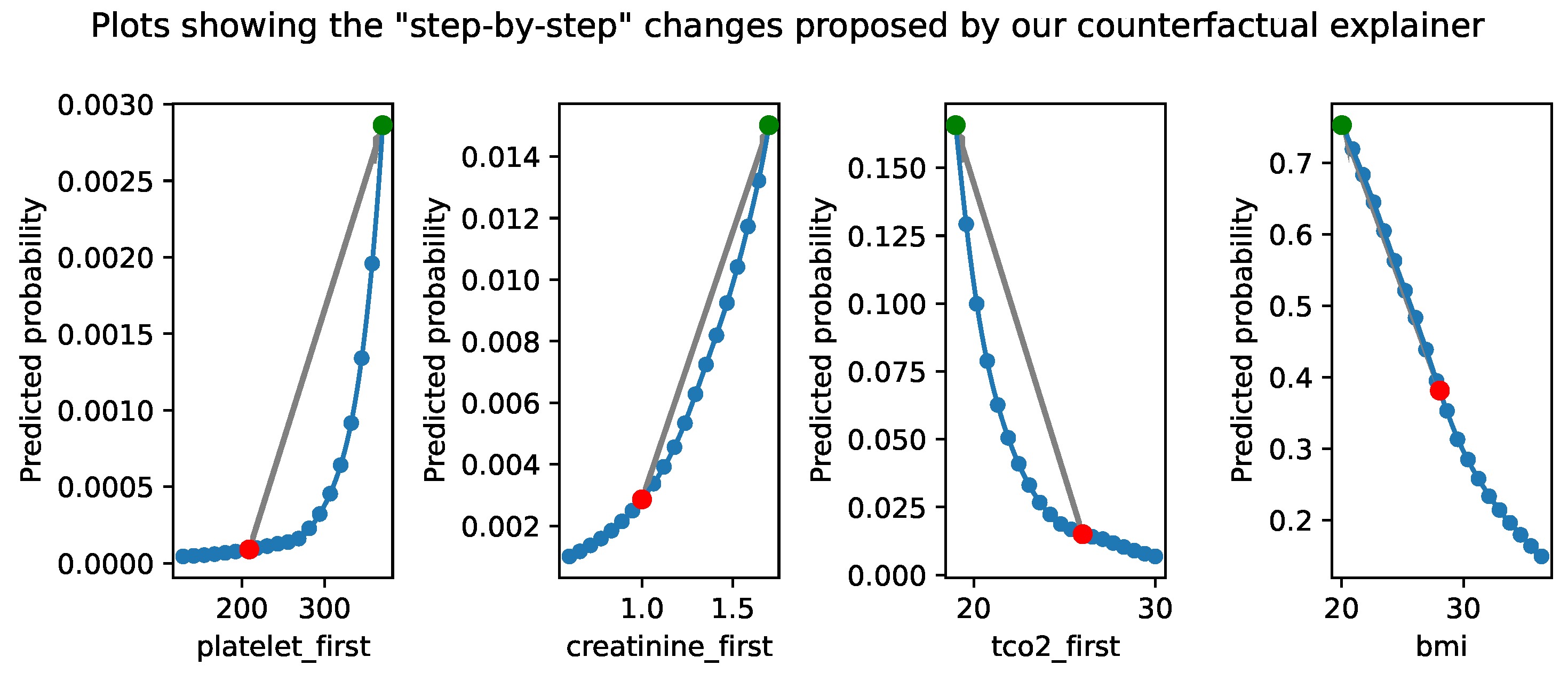
Figure 5 shows the counterfactuals generated by our methodology. These counterfactuals are plausible, i.e. taking realistic values for the variables present (we discuss possible correlation within the variables making this not realistic in our Future Work section). They are also unambiguous — they clearly show a change in classification, increasing the probability of death from
to
.
This presentation of our results highlights a key benefit of our methodology, that it creates sequential counterfactuals. This means that it gives a series of steps that a user can take to change the model’s output. This is particularly useful in medical situations, as these can often be actionable where a user (such as a clinician) can take these steps to improve the patient’s health. We can use changeability scores to tailor our results here, by assigning higher scores to the features we want to change. For example, we can assign a higher score to the weight feature, as this is something that is easier to change than the age feature. As these scores would be different for each patient, our method allows for a domain expert (such as a clinician) to tune this in a human-in-the-loop fashion.
4.2. Financial Data-Set
4.2.1. Qualitative Evaluation and Complex Narratives
We qualitatively evaluate the performance of our methodology on financial data.
Beginning with equal changeability scores on the applicant described in
Table 2, (with an additional threshold of
and 20 samples used to train each surrogate model) suggests that the applicant should have a higher income (
Figure 6). However, this may not be useful to an applicant, as this is not actionable. By setting this variable’s changeability score to zero, we can use our methodology to get more practically useful results.
For sake of example, let us also suppose that the applicant cannot change the size of the loan they are applying for, nor their age, nor their housing situation. In this situation, our model was unable to generate a counterfactual.
This intuitive process for setting these changeability scores, allows for the generation of complex narratives to explain the decisions of machine learning models (in human interpretable ways) [
68]. This result suggests that the model (which approximates the automated decision-making system), is highly dependent on opaque and/or fixed features. Thus, our approach offers an understanding of how the model makes decisions, which can help in creating fair models.
Included in
Table 4, is an example of an applicant who our model predicted should be awarded the loan. We can ask the question “why should they be awarded the loan?” by finding counterfactuals which would not be awarded the loan. As shown in
Figure 7, our method says that the applicant would not be awarded the loan if they had a lower income.
We can again use changeability scores to get more tailored explanations. For example, if we restrict what features can be changed to only “length of employment”, “interest rate”, “credit history length”, and “age” (overall, roughly equivalent to applying for the loan later), we are still able to generate a counterfactual. We have included this below:
4.3. Image Dataset
We applied our methodology, alongside other points of comparison previously discussed, to the MNIST dataset. We use linear surrogate models and allowing features to take values between the and quantiles of the training data.
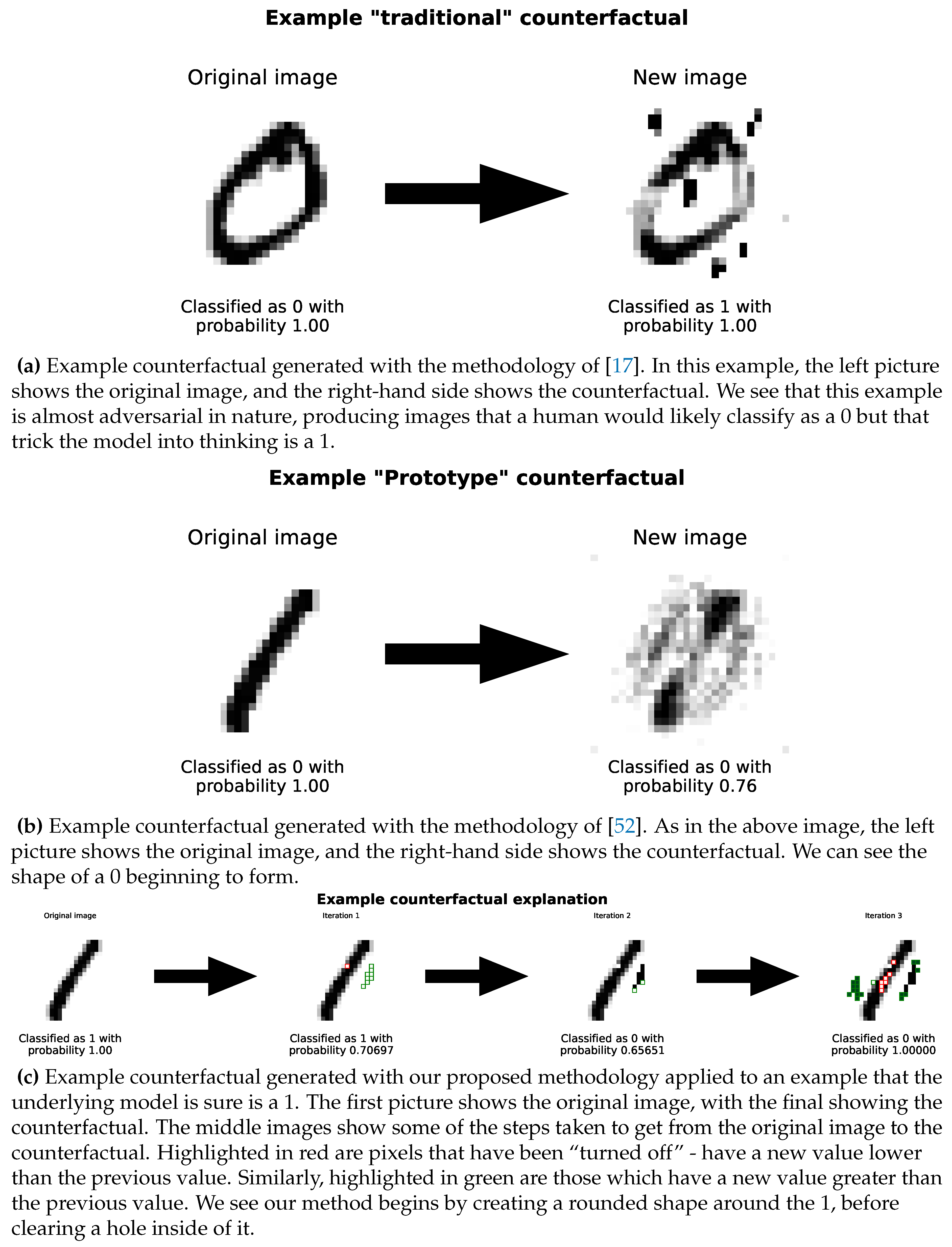
We can see a step-by-step example of this in
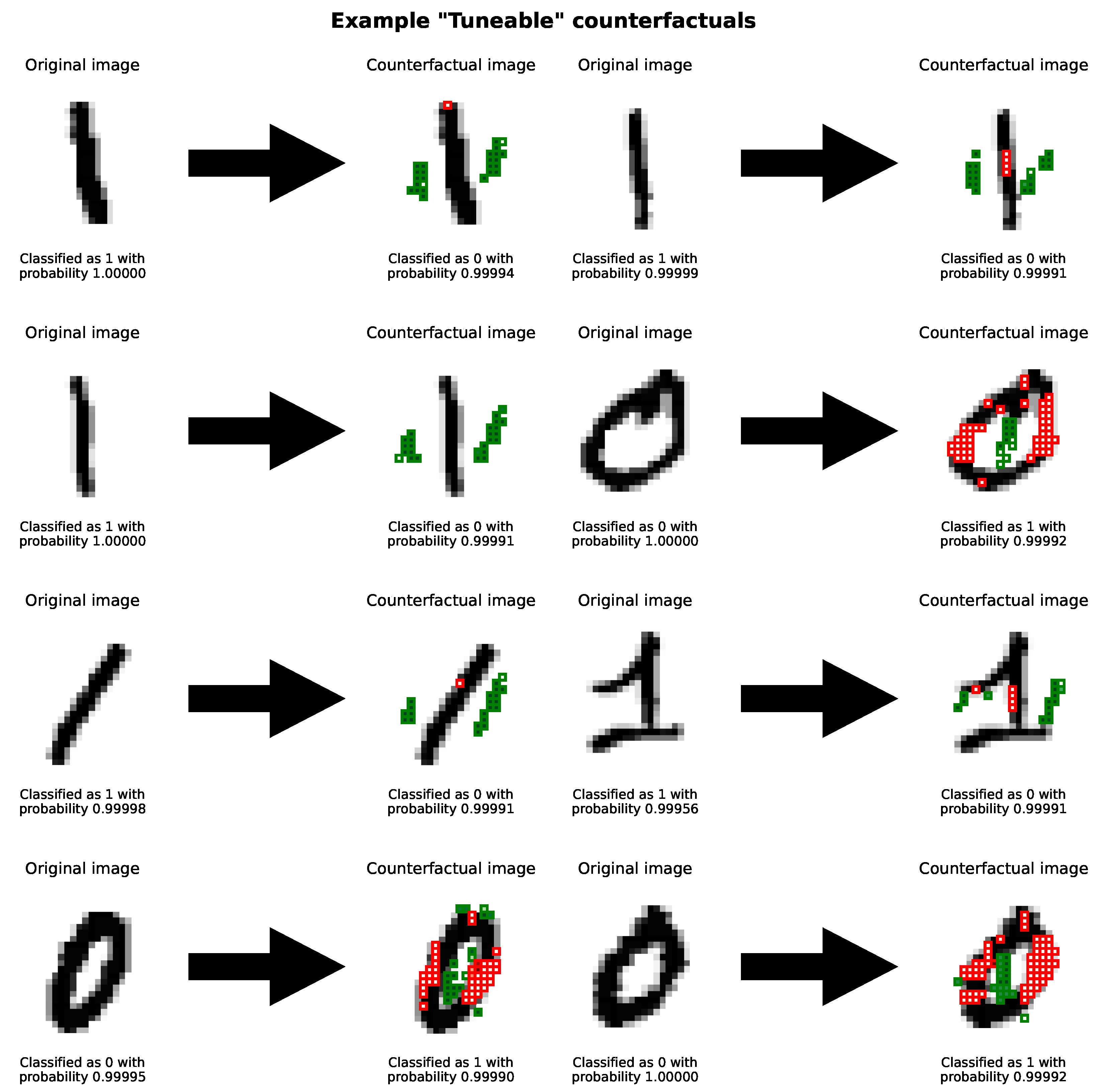
Figure 8c. Further examples are included in
Figure 9
These counterfactuals give us insight into how the model makes its classification decisions. In some sense, it begins to “cut-open” the 1 to make it look more like a 0.
Similarly, running the previously described existing methodologies on this example, lead to different, almost adversarial counterfactuals. These are shown in
Figure 8a and
Figure 8b.
We can see a clear qualitative difference in the types of counterfactual generated between our methodology and the two comparison methods. In a sense, our method works more to transform the image from a 0 into a 1, while the other methods work to perturb the image from a 0 into a 1. Since our method chains together single pixel changes, there is an inbuilt incentive for our method to change fewer pixels (as each change is costed by the scoring function). This is not the case for the other methods, which can change many pixels at once. This can lead to our counterfactuals being more human-interpretable.
Similarly, our use of changeability scores can be used as an alternative method to guide counterfactuals to be more interpretable. For example, when generating our MNIST counterfactuals, we want to change pixels close to the digit. We can do this by giving these pixels a higher changeability score. We do this by blurring the image, and applying a threshold of
to these scores. This is shown in
Figure 11. This continues to generate counterfactuals that are close to the original image, but also interpretable, demonstrating the flexibility of our methodology. Similarly, our counterfactuals are unambiguous — they demonstrate a clear change in classification. Another example is shown in
Figure 12.
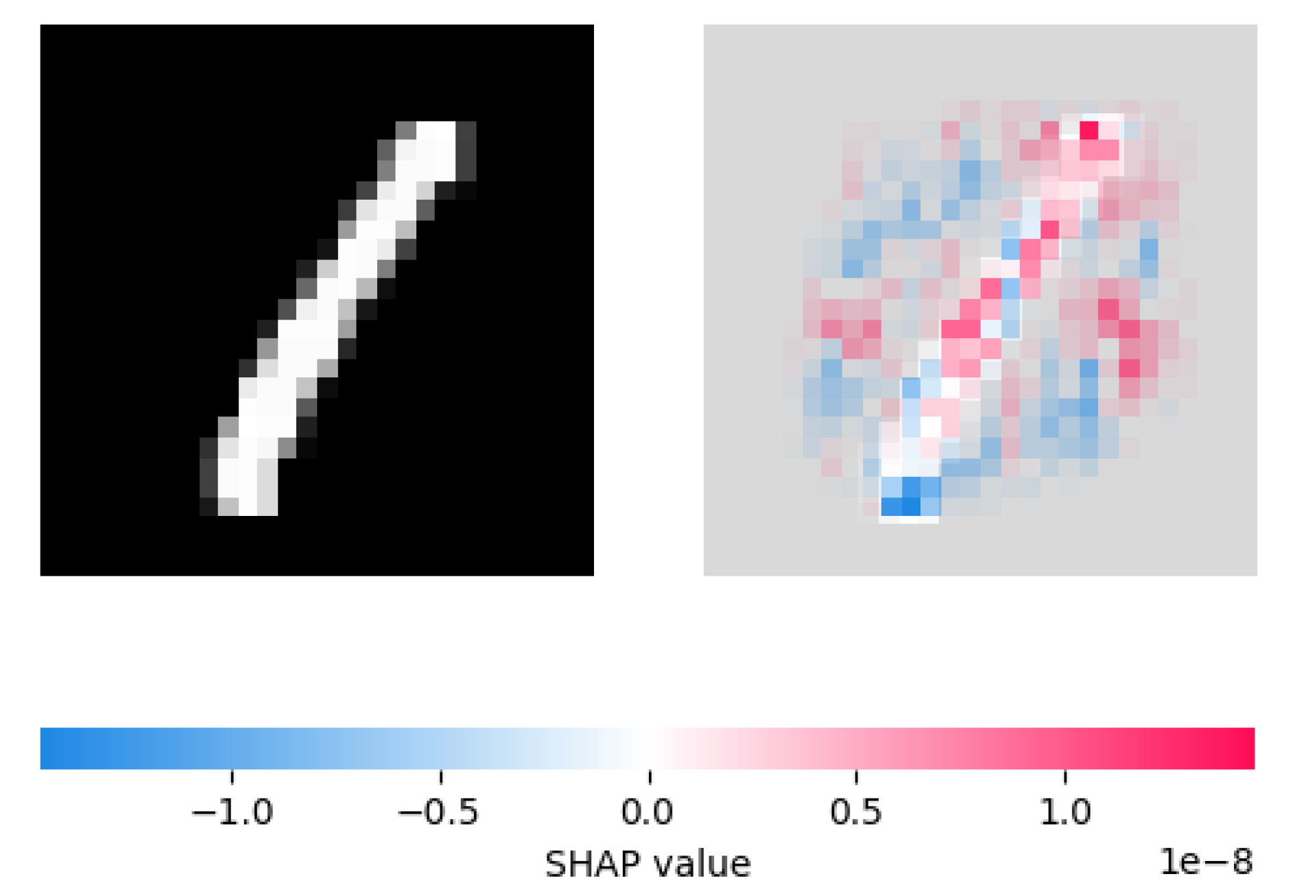
4.3.1. Comparison with SHAP
As our idea of fitting linear surrogate models is somewhat similar to SHAP values, we include a comparison with SHAP values in
Figure 10.
We see that, in this example, the SHAP explainer assigns high importance values to similar areas of the image as our counterfactual explainer chooses to change. In some sense, this is unsurprising considering the similarities between our methodologies.
Figure 11.
Example counterfactual generated with our methodology using changeability scores derived from a Gaussian blur. We have applied our method to a image originally classified as a 1. We see that, to generate our changeability scores, we first blue the image with a Gaussian, then apply a threshold to the these scores. Using these we are able to produce a simple counterfactual which the model believes is a 0 with probability 0.64. We see that it has created a hole in the centre of the 1, suggesting that the model using this is as a classification criteria
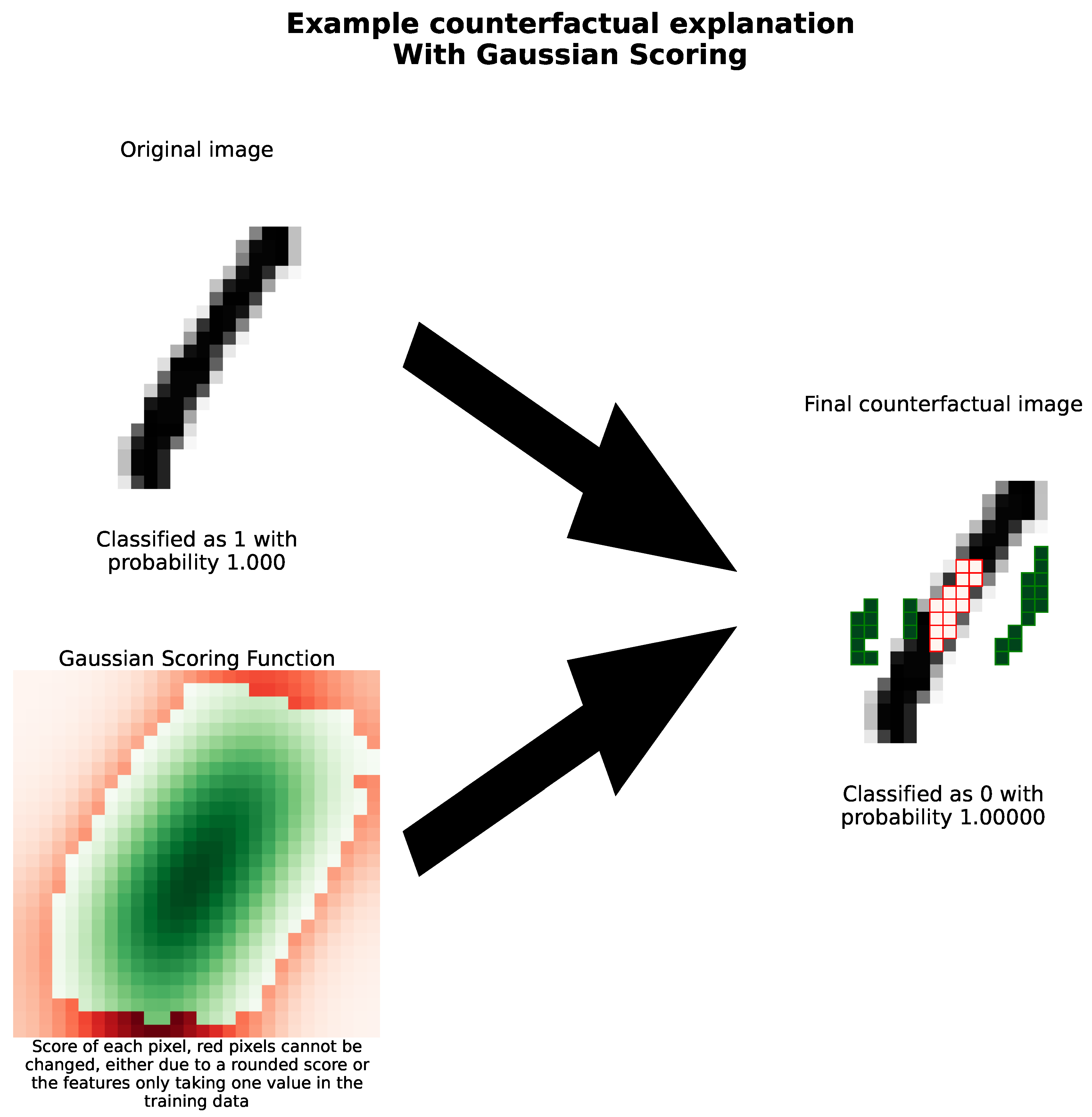
Figure 12.
Example counterfactual generated with our methodology. Here, we use the Gaussian scoring function on an image that the underlying model is convinced is a 0 and use our method to transform it into an image that the underlying model is sure is a 1. The top-left picture shows the original image, with the right image showing the counterfactual. In the final image, highlighted in red are pixels which have been turned off - have a new value lower than the previous value. Similarly, highlighted in green are those which have a new value greater than the previous value. We see again that our method begins by attempting to fill in the 0, suggesting the underlying model uses the hole as a classification criteria. The bottom-left image shows our Gaussian scoring function, with the darker pixels showing a higher changeability score. While most of the pixels are in green, the red pixels represent pixels that our method will not change - either because their changeability score has been rounded to zero, or because they do not take a range of values in the training dataset.
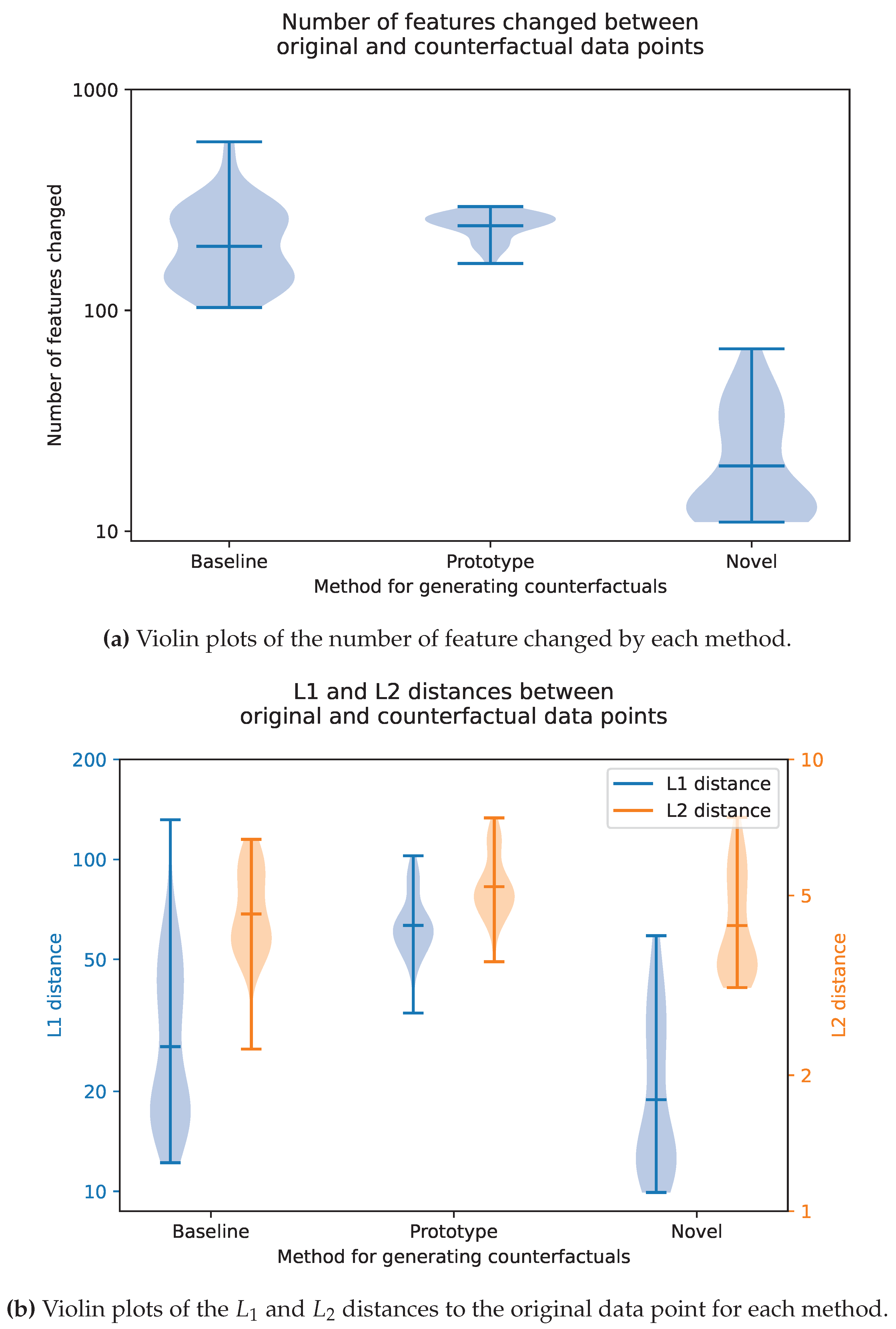
4.4. Quantitative Evaluations
Figure 13 shows violin plots of the various quantitative metrics defined in
Section 3.3.1. To generate these quantitative results, we randomly sampled 50 images from the original MNIST training dataset. We applied our methodology, and comparable methodologies, to these examples, with a
linear regressor and a
quantile bounding method. We then quantitatively compared the counterfactuals generated.
As shown in these plots, compared to comparable methods, our proposed methodology changes fewer features, but changes them by a larger amount (both in terms of and distance). In a sense, our counterfactuals are more interpretable, since they change fewer features.
5. Conclusions
5.1. Key Contributions
In this work, we develop a methodology to generate counterfactuals to explain black-box models. This method borrows ideas from human-computer interaction research to develop a tuneable, human-in-the-loop explanation method for machine learning models.
From a technical lens, our method can perform on any black box model. Similarly, our method can easily be parallelised at each stage of the search process (
Figure 3). Similarly, our system produces sequential counterfactuals (which end-users strongly prefer and regard as more trustworthy [
47]).
Furthermore, our code structure is very flexible – not only can any regressor be used for the single-variable explainers, but we also build in various “scoring functions” that provide different counterfactuals for different use cases. For example, our
searcher system could be modified to not attempt to try and change conflicting features - such as the various housing indicator columns in
Table 2. Through the use of changeability scores, our method provides an inherent tuneability that makes it useful in a range of settings. Similarly, by following a step-by-step process, with each step being an inherently explainable model, our explanations are easily interpretable to a non-technical user.
We also see that our method is able to work on a range of input formats, and applications. Here, we show that our approach can work on both tabular and image formats. We show specific applications in the fields of finance, medicine and image recognition.
We evaluated the performance of our approach on a range of data sets. We found that our approach is able to produce, on average, counterfactuals that change fewer features, and change these by larger amounts. Overall, we have shown some benefits of our method compared to some existing methods for generating counterfactuals.
We hope our method can find broad applicability in critical domains such as finance and healthcare, where explainability is important.
5.2. Limitations and Future Work
Our methodology relies on fitting models to the variation of individual features. However, this cannot account for the correlation between different features. One possible methodology for addressing this is to allow a domain expert to form groups of features likely to be correlated and fit simple models to these. By using the training data itself to guide what values are allowed – possibly through an auto-encoder – we can account for these correlations. Similarly, we could implement different strategies into our search method (
Figure 3).
There is also scope to conduct extensive user studies into how both how domain experts understand the tunability of our method and how well users respond to the counterfactuals generated. This will be the subject of future work.
We note that our model only aims to change the decisions made by a model, not the “ground truth”. A particular example of this is that, in the case of handwritten digits, we have not changed a 1 to a 0, as any human looking at the images would still believe this is a 1. We have only changed the decision made by the model. This is a limitation of any explainable AI method, including ours.
Ethics: No ethics approval was necessary for this work.
Code availability: All code used in this work is available from the following repository:
https://github.com/JoshanParmar/TuneableCounterfactuals
Our python package can be installed using pip through
pip install tuneable-counterfactuals-explainer
Conflicts of Interest
All authors declare they have no conflicts of interest to disclose.
Data Availability Statement
This study does not generate any data.
Author Contributions
JP carried out the implementation and analysis, participated in the design of the study and wrote the manuscript. PL carried out the analysis and participated in the design of the study. SB carried out the analysis, participated in the design of the study and wrote the manuscript. SB directed the study. All authors gave final approval for publication.
Funding
SB acknowledges funding from the Accelerate Programme for Scientific Discovery Research Fellowship. The funders had no role in study design, data collection and analysis, decision to publish, or preparation of the manuscript. The views expressed are those of the authors and not necessarily those of the funders.
References
- Molnar, C. Interpretable Machine Learning; Independently published, 2023.
- Castelvecchi, D. Can we open the black box of AI? Nature News 2016, 538, 20. [Google Scholar] [CrossRef] [PubMed]
- Lundberg, S. slundberg/shap, 2023. original-date: 2016-11-22T19:17:08Z.
- Ribeiro, M.T.; Singh, S.; Guestrin, C. "Why Should I Trust You?": Explaining the Predictions of Any Classifier, 2016. arXiv:1602.04938.
- Office of Ron Wyden. Algorithmic Accountability Act of 2022 One-Pager. Technical report, Office of Ron Wyden, 2022.
- Ramakrishnan, G.; Lee, Y.C.; Albarghouthi, A. Synthesizing Action Sequences for Modifying Model Decisions. Proceedings of the AAAI Conference on Artificial Intelligence 2020, 34, 5462–5469. [Google Scholar] [CrossRef]
- Allen, D.M.W.a.J.R. How artificial intelligence is transforming the world, 2018.
- Gibbons, S. 2023 Business Predictions As AI And Automation Rise In Popularity, 2023. Section: Entrepreneurs.
- Islam, M.R.; Ahmed, M.U.; Barua, S.; Begum, S. A Systematic Review of Explainable Artificial Intelligence in Terms of Different Application Domains and Tasks. Applied Sciences 2022, 12, 1353. [Google Scholar] [CrossRef]
- Lundberg, S.M.; Lee, S. A unified approach to interpreting model predictions. CoRR 2017, abs/1705.07874, [1705.07874].
- Zhou, B.; Khosla, A.; Lapedriza, A.; Oliva, A.; Torralba, A. Learning Deep Features for Discriminative Localization, 2015. arXiv:1512.04150.
- Koh, P.W.; Nguyen, T.; Tang, Y.S.; Mussmann, S.; Pierson, E.; Kim, B.; Liang, P. Concept Bottleneck Models, 2020. arXiv:2007.04612.
- Towards Automatic Concept-based Explanations, 2019. arXiv:1902.03129 [cs, stat]. [CrossRef]
- Yeh, C.K.; Kim, B.; Arik, S.; Li, C.L.; Pfister, T.; Ravikumar, P. On Completeness-aware Concept-Based Explanations in Deep Neural Networks. In Proceedings of the Advances in Neural Information Processing Systems. Curran Associates, Inc., 2020, Vol. 33, pp. 20554–20565.
- Banerjee, S.; Lio, P.; Jones, P.B.; Cardinal, R.N. A class-contrastive human-interpretable machine learning approach to predict mortality in severe mental illness. npj Schizophrenia 2021 7:1 2021, 7, 1–13. [Google Scholar] [CrossRef]
- Lash, M.T.; Lin, Q.; Street, W.N.; Robinson, J.G.; Ohlmann, J.W. Generalized Inverse Classification. CoRR 2016, abs/1610.01675, [1610.01675].
- Wachter, S.; Mittelstadt, B.; Russell, C. Counterfactual Explanations Without Opening the Black Box: Automated Decisions and the GDPR, 2017. Place: Rochester, NY Type: SSRN Scholarly Paper. [CrossRef]
- Guidotti, R. Counterfactual explanations and how to find them: literature review and benchmarking. Data Mining and Knowledge Discovery 2022. [Google Scholar] [CrossRef]
- Kingma, D.P.; Ba, J. Adam: A Method for Stochastic Optimization. arXiv 2017. [Google Scholar] [CrossRef]
- Powell, M.J.D. On search directions for minimization algorithms. Mathematical Programming 1973, 4, 193–201. [Google Scholar] [CrossRef]
- Verma, S.; Boonsanong, V.; Hoang, M.; Hines, K.E.; Dickerson, J.P.; Shah, C. Counterfactual Explanations and Algorithmic Recourses for Machine Learning: A Review. arXiv 2022. [Google Scholar] [CrossRef]
- Tolomei, G.; Silvestri, F.; Haines, A.; Lalmas, M. Interpretable Predictions of Tree-based Ensembles via Actionable Feature Tweaking. In Proceedings of the Proceedings of the 23rd ACM SIGKDD International Conference on Knowledge Discovery and Data Mining, Halifax NS Canada, 2017; pp. 465–474. [CrossRef]
- Carreira-Perpiñán, M.Á.; Hada, S.S. Counterfactual Explanations for Oblique Decision Trees:Exact, Efficient Algorithms. Proceedings of the AAAI Conference on Artificial Intelligence 2021, 35, 6903–6911. [Google Scholar] [CrossRef]
- Lucic, A.; Oosterhuis, H.; Haned, H.; de Rijke, M. FOCUS: Flexible Optimizable Counterfactual Explanations for Tree Ensembles, 2021. arXiv:1911.12199.
- Russell, C. Efficient Search for Diverse Coherent Explanations. In Proceedings of the Proceedings of the Conference on Fairness, Accountability, and Transparency, Atlanta GA USA, 2019; pp. 20–28. [CrossRef]
- Ustun, B.; Spangher, A.; Liu, Y. Actionable Recourse in Linear Classification. In Proceedings of the Proceedings of the Conference on Fairness, Accountability, and Transparency, Atlanta GA USA, 2019; pp. 10–19. [CrossRef]
- Fernández, R.R.; Martín de Diego, I.; Aceña, V.; Fernández-Isabel, A.; Moguerza, J.M. Random forest explainability using counterfactual sets. Information Fusion 2020, 63, 196–207. [Google Scholar] [CrossRef]
- Ho, T.K. Random decision forests. In Proceedings of the Proceedings of 3rd International Conference on Document Analysis and Recognition, 1995, Vol. 1, pp. 278–282 vol.1. [CrossRef]
- Cui, Z.; Chen, W.; He, Y.; Chen, Y. Optimal Action Extraction for Random Forests and Boosted Trees. In Proceedings of the Proceedings of the 21th ACM SIGKDD International Conference on Knowledge Discovery and Data Mining, Sydney NSW Australia, 2015; pp. 179–188. [CrossRef]
- Freund, Y.; Schapire, R.E. A Decision-Theoretic Generalization of On-Line Learning and an Application to Boosting. Journal of Computer and System Sciences 1997, 55, 119–139. [Google Scholar] [CrossRef]
- Friedman, J.H. Greedy Function Approximation: A Gradient Boosting Machine. The Annals of Statistics 2001, 29, 1189–1232, Publisher: Institute of Mathematical Statistics. [Google Scholar] [CrossRef]
- Laugel, T.; Lesot, M.J.; Marsala, C.; Renard, X.; Detyniecki, M. Comparison-Based Inverse Classification for Interpretability in Machine Learning. In Proceedings of the Information Processing and Management of Uncertainty in Knowledge-Based Systems. Theory and Foundations; Medina, J.; Ojeda-Aciego, M.; Verdegay, J.L.; Pelta, D.A.; Cabrera, I.P.; Bouchon-Meunier, B.; Yager, R.R., Eds., Cham, 2018; Communications in Computer and Information Science, pp. 100–111. [CrossRef]
- Dhurandhar, A.; Chen, P.Y.; Luss, R.; Tu, C.C.; Ting, P.; Shanmugam, K.; Das, P. Explanations based on the Missing: Towards Contrastive Explanations with Pertinent Negatives, 2018. arXiv:1802.07623.
- Dhurandhar, A.; Pedapati, T.; Balakrishnan, A.; Chen, P.Y.; Shanmugam, K.; Puri, R. Model Agnostic Contrastive Explanations for Structured Data, 2019. arXiv:1906.00117 [cs, stat].
- Beck, A.; Teboulle, M. A Fast Iterative Shrinkage-Thresholding Algorithm for Linear Inverse Problems. SIAM Journal on Imaging Sciences 2009, 2, 183–202, Publisher: Society for Industrial and Applied Mathematics. [Google Scholar] [CrossRef]
- Guidotti, R.; Monreale, A.; Ruggieri, S.; Pedreschi, D.; Turini, F.; Giannotti, F. Local Rule-Based Explanations of Black Box Decision Systems, 2018. arXiv:1805.10820 [cs].
- Dandl, S.; Molnar, C.; Binder, M.; Bischl, B. Multi-Objective Counterfactual Explanations. In Proceedings of the Parallel Problem Solving from Nature – PPSN XVI. Springer International Publishing, 2020, pp. 448–469. [CrossRef]
- Duong, T.D.; Li, Q.; Xu, G. Causality-based Counterfactual Explanation for Classification Models, 2023. arXiv:2105.00703 [cs].
- Van Looveren, A.; Klaise, J. Interpretable Counterfactual Explanations Guided by Prototypes, 2020. arXiv:1907.02584 [cs, stat].
- Jordan, J. Introduction to autoencoders., 2018.
- Kanamori, K.; Takagi, T.; Kobayashi, K.; Arimura, H. DACE: Distribution-Aware Counterfactual Explanation by Mixed-Integer Linear Optimization. In Proceedings of the Proceedings of the Twenty-Ninth International Joint Conference on Artificial Intelligence, Yokohama, Japan, 2020; pp. 2855–2862. [CrossRef]
- Mahalanobis, P.C. On the Generalised Distance in Statistics, 1936.
- Breunig, M.M.; Kriegel, H.P.; Ng, R.T.; Sander, J. LOF: Identifying Density-Based Local Outliers. SIGMOD Rec. 2000, 29, 93–104. [Google Scholar] [CrossRef]
- Mahajan, D.; Tan, C.; Sharma, A. Preserving Causal Constraints in Counterfactual Explanations for Machine Learning Classifiers, 2020. arXiv:1912.03277 [cs, stat].
- Xiang, X.; Lenskiy, A. Realistic Counterfactual Explanations with Learned Relations, 2022. arXiv:2202.07356 [cs, stat].
- Kingma, D.P.; Welling, M. Auto-Encoding Variational Bayes, 2022. arXiv:1312.6114 [cs, stat]. [CrossRef]
- Singh, R.; Miller, T.; Lyons, H.; Sonenberg, L.; Velloso, E.; Vetere, F.; Howe, P.; Dourish, P. Directive Explanations for Actionable Explainability in Machine Learning Applications. ACM Transactions on Interactive Intelligent Systems 2023, p. 3579363. [CrossRef]
- Naumann, P.; Ntoutsi, E. Consequence-Aware Sequential Counterfactual Generation. In Proceedings of the Machine Learning and Knowledge Discovery in Databases. Research Track; Oliver, N.; Pérez-Cruz, F.; Kramer, S.; Read, J.; Lozano, J.A., Eds., Cham, 2021; Lecture Notes in Computer Science, pp. 682–698. [CrossRef]
- Van Rossum, G.; Drake Jr, F.L. Python tutorial; Centrum voor Wiskunde en Informatica Amsterdam, The Netherlands, 1995.
- Klaise, J.; Van Looveren, A.; Vacanti, G.; Coca, A. Alibi Explain: Algorithms for Explaining Machine Learning Models, 2021.
- Parmar, J. Tuneable Counterfactuals; GitHub, 2024.
- Van Looveren, A.; Klaise, J.; Vacanti, G.; Cobb, O. Conditional Generative Models for Counterfactual Explanations, 2021.
- Inam, R.; Terra, A.; Fersman, E.; Feljan, A.V. Explainable AI: How humans can trust Artificial Intelligence, 2021.
- Blackwell, A. Bias and Fairness, 2022. Place: University of Cambridge.
- Goodman, B.; Flaxman, S. European Union Regulations on Algorithmic Decision-Making and a “Right to Explanation”. AI Magazine 2017, 38, 50–57, Publisher: Wiley. [Google Scholar] [CrossRef]
- Wiyatno, R.R.; Xu, A.; Dia, O.; de Berker, A. Adversarial Examples in Modern Machine Learning: A Review. CoRR 2019, abs/1911.05268, [1911.05268].
- Nemirovsky, D.; Thiebaut, N.; Xu, Y.; Gupta, A. CounteRGAN: Generating counterfactuals for real-time recourse and interpretability using residual GANs. In Proceedings of the Proceedings of the Thirty-Eighth Conference on Uncertainty in Artificial Intelligence. PMLR, 2022, pp. 1488–1497. ISSN: 2640-3498.
- Goodfellow, I.; Pouget-Abadie, J.; Mirza, M.; Xu, B.; Warde-Farley, D.; Ozair, S.; Courville, A.; Bengio, Y. Generative Adversarial Nets. In Proceedings of the Advances in Neural Information Processing Systems. Curran Associates, Inc., 2014, Vol. 27.
- Pedregosa, F.; Varoquaux, G.; Gramfort, A.; Michel, V.; Thirion, B.; Grisel, O.; Blondel, M.; Prettenhofer, P.; Weiss, R.; Dubourg, V.; et al. Scikit-learn: Machine Learning in Python. Journal of Machine Learning Research 2011, 12, 2825–2830. [Google Scholar]
- Chollet, F.; et al. Keras. https://keras.io, 2015.
- Warren, G.; Keane, M.T.; Byrne, R.M.J. Features of Explainability: How users understand counterfactual and causal explanations for categorical and continuous features in XAI, 2022, [arXiv:cs.HC/2204.10152].
- pandas development team, T. pandas-dev/pandas: Pandas, 2023. [CrossRef]
- Schut, L.; Key, O.; McGrath, R.; Costabello, L.; Sacaleanu, B.; Corcoran, M.; Gal, Y. Generating Interpretable Counterfactual Explanations By Implicit Minimisation of Epistemic and Aleatoric Uncertainties. arXiv 2021.
- Tse, L. Credit Risk Dataset, 2020.
- Saeed, M.; Villarroel, M.; Reisner, A.; Clifford, G.; Lehman, L.w.; Moody, G.; Heldt, T.; Kyaw, T.; Moody, B.; Mark, R. MIMIC-II Clinical Database, 2011. [CrossRef]
- Raffa, J. Clinical data from the MIMIC-II database for a case study on indwelling arterial catheters:, 2016. [CrossRef]
- Deng, L. The mnist database of handwritten digit images for machine learning research. IEEE Signal Processing Magazine 2012, 29, 141–142. [Google Scholar] [CrossRef]
- Banerjee, S. Generating Complex Explanations for Artificial Intelligence Models: An Application to Clinical Data on Severe Mental Illness. Life 2024, Vol. 14, Page 807 2024, 14, 807. [CrossRef]
|
Disclaimer/Publisher’s Note: The statements, opinions and data contained in all publications are solely those of the individual author(s) and contributor(s) and not of MDPI and/or the editor(s). MDPI and/or the editor(s) disclaim responsibility for any injury to people or property resulting from any ideas, methods, instructions or products referred to in the content. |
© 2025 by the authors. Licensee MDPI, Basel, Switzerland. This article is an open access article distributed under the terms and conditions of the Creative Commons Attribution (CC BY) license (http://creativecommons.org/licenses/by/4.0/).