
Submitted:
14 October 2025
Posted:
15 October 2025
You are already at the latest version
Abstract
Agriculture and robotics have managed to integrate, using artificial intelligence in plant tracking and pest detection, as well as robotic arms and remote-controlled robots for harvesting, significantly reducing the human workload. Robots are typically designed to perform specific tasks, making their adaptability very difficult to integrate into agriculture due to the constant changes of plants, such as plant growth. As a result of the general and current functions in agro-robotics, continuous monitoring with deep learning is aimed at knowing the condition of the plants and that the mobility of the robots does not impede the plant’s growth while being monitored for it to adapt to the monitoring environment. Deep learning and a robotic arm are used for real-time plant monitoring. Image database will be used for training, accuracy, recall and F1 indicators are used to evaluate the network. The robot has kinematics that allows it to change its size to monitor plant health and growth. Early detection of plant leaf anomalies and diseases using a deep learning system. Integrating the various systems, provided an intelligent and effective solution for detecting anomalies and diseases in the leaves of plants subjected to intelligent robotic monitoring.
Keywords:
agricultural robotics
; plant health monitoring
; deep learning
; computer vision
; robotic arm
; real-time monitoring
; leaf disease detection
; precision agriculture
1. Introduction
To meet the Sustainable Development Goals (SDG) related to access to nutritious and healthy food, the agricultural sector plays a key role. Between 2000 and 2021, global vegetable production grew by 68 %, reaching a total volume of 1.150 million tons in 2021. The most produced vegetable was tomato (189 million tons in 2021), followed by onion (107 million tons) and cucumbers (93 million tons) (FAO, 2022). The countries with the highest production of tomato (Solanum lycopersicon) were China (67.538.340,00 tons), India (21.181.000,00 tons) and Turkey (13.095.258,00 tons). In South America, tomato production was 7.27 million tons. Particularly, Honduras had a production of 75.972,12 tons, ranking 85th (FAO, 2023). Global tomato production is expected to continue increasing, especially that obtained from greenhouse crops. This is due to the almost ideal conditions achieved: shorter maturity rate, high productivity per unit area and prolonged production phase (Tao et al., 2016). In addition, crops grown in greenhouse conditions are less prone to attacks by pests and diseases. The above favors the production of tomato crops, since it is one of the vegetables most attacked by pests and diseases. Therefore, its cultivation is produced through the application of many chemical products. The use of these chemical products affects the farmer, the consumer, and the environment, which is why today, organic cultivation is promoted. The above does not affect the quality of the fruit and the quantity of production (Karungi et al., 2011). In addition to the use of chemical methods to manage pests and diseases, one of the activities carried out to control the appearance of these, is the exploration of crops. These explorations make it possible to identify both the appearance and the type of pests and diseases, allowing the measures to be adopted to be determined. This requires observing, identifying, monitoring, recording, and recommending the actions to be taken. However, the exploration is an activity that requires a large amount of time and effort and is prone to human errors (Lin and Guo, 2020). Thus, in recent years, the evolution of technology has generated innovative instruments and methodologies to be used in agriculture. This generated the paradigm of Precision Agriculture (PA) that seeks to manage the agricultural production process in an innovative way; carrying out activities such as: monitoring the status of the plants; control of weeds, pests, and diseases; monitoring of soil nutritional variables; application of agronomic inputs; to have better production; to have more outstanding production in terms of plant growth; among others [2] (Avola et al., 2024). Some of the technologies that have been incorporated in the agricultural sector are: 1) robotic systems as: unmanned aerial systems (UAS) (Lin & Guo, 2020), unmanned robots [3], and others (Gao et al., 2024; Ling et al., 2019); 2) Big-data (More et al., 2019); 3) Artificial Intelligence (AI) (Sheikh et al., 2023); 4) Cloud Computing technologies (Xia et al., 2021); 5) Computer Vision (Rong et al., 2023) and the combination of them (Zhang et al., 2023; Rong et al., 2022; Yu et al., 2021). One of the applications in which these technologies are used is the early detection of foliar diseases, to avoid losses in crop production, and therefore, economic losses [4]. The goal of plant disease detection is to prevent, control and eliminate damage caused by pathogens and stressors, thereby protecting plant health, and ensuring crop safety. The advantage of early detection is that it allows appropriate measures to be taken to prevent diseases and minimize crop losses [5].
We have developed a robot capable of detecting plant leaf health by combining advanced technology. Detecting health problems that can identify diseases, nutritional deficiencies, and pests in plant leaves early and accurately is crucial to prevent the spread of problems and maintain crop health. The robotic arm with its degrees of freedom will be able to provide precise and controlled movements, thereby offering a more stable platform as stability is essential for monitoring activities that require precise positioning. The robot will be designed with an end effector that along with stability will be able to collect specific data.
An artificially intelligent robot designed for leaf disease detection offers significant advantages to an agricultural industry that is largely inefficient in terms of labor and relies heavily on the use of fertilizers without specific data on plant health. With this robot, it will be possible to detect diseases early to know what measures to take for good plant care, in addition to reducing the use of pesticides, there will also be a control with which crop production will be of better quality. This will eliminate the need for manual inspections, which will save more time to prevent leaf diseases, and will ensure better plant growth and safer, higher quality food production.
Figure 1.
Tuning result for test 2
2. State of Art
As consumers demand increasingly higher quality standards for agricultural products, inspection of agricultural products has become an integral component of the farming production process [1]. Increasing the rate of food production requires automation, robotics, information, and intelligence services that combine information and communication technologies (ICT), robotics, artificial intelligence (AI), big data, and the Internet of Things [2]. Redundant robots are essential because they allow us to perform more complicated and flexible tasks. They can avoid obstacles and singularities and optimize torque while reaching the target position with good precision [3]. The growing demand for quality agricultural products drives the integration of emerging technologies such as the Internet of Things in agriculture. This shift towards "smart farming" redefines methods with quantitative approaches.
The work collaboration between humans and robots has worked positively; this has as an objective a good collaboration between robots and humans to reach a higher productivity thanks to the joint action between human intelligence and the mechanical power of a robot [4]. For robots to be successful in intelligent manufacturing environments, it is essential that they can precisely manage how they move and how they physically interact [5]. The time required to perform a pick-and-place operation is subject to multiple factors, including the kinematic configuration of the robot, its inertial properties, and the characteristics of the drive and transmission systems, which set limits on the maximum achievable speed and acceleration [6]. Practical human-robot cooperation aims to boost output by fusing human intellect with robotics mechanical prowess, focusing on accurate motion control and hands-on interaction in intelligent production settings.
Reasonable control and programming in a redundant manipulator lie in its ability to avoid collisions with the environment and maintain safety in machine-human collaboration [7]. A trajectory planning technique is suggested that improves efficiency by avoiding unnecessary solutions and judgments; comparative testing in a problematic environment demonstrates the effectiveness of the suggested method [8]. A recent study examines an adaptive fuzzy recurrent neural network (AFRNN) model to solve the non-repetitive motion problem of redundant robotic manipulators; the convergence parameters of the AFRNN are self-adaptive [9]. Path planning techniques and adaptive neural network models have been suggested to enhance efficiency, and their efficacy under challenging environments has been demonstrated.
Today, robotic manipulators must operate in a dynamic environment and perform increasingly complex and precise tasks. For this reason, robots are used that have more degrees of freedom than the desired task requires [10]. In robotics, the contact force of the end effector with the target influences the robot’s structure [11]. A robotic manipulator can be equipped with different end effectors to perform various tasks. Grippers are one of the most commonly used robot arm-end tools. Depending on the application of the robotic system, multiple types of grippers are needed [12]. Redundant manipulators offer unique versatility when tackling complex tasks. Its ability to adopt numerous configurations and orientations, exceeding the required degrees of freedom, demonstrates unmatched flexibility.
In formulating a non-linear optimization problem to solve the inverse kinematics problem in redundant robots, the quadratic programming (QP) technique is used to include joint constraints and reduce the kinetic energy of the robot [13]. A finite-time convergence adaptive fuzzy control scheme for double-arm robots with uncertain kinematics and dynamics is presented in this research; it is a control scheme that addresses the problems of controlling redundant robots with complex structures and mechanisms [14]. Optimization alternatives like K routes are frequently employed in robotics and automation to determine the quickest and most effective way for a robot to go [15]. These investigations present promising solutions for optimizing inverse kinematics, improving the precision of movements, and addressing the challenges of robots with complex structures.
Artificial neural networks have shown great promise in implementing recognition and classification applications [16]. Neural networks have been used and improved in various applications, such as object recognition, image restoration, combination optimization, and large-scale embedded matrices [17]. Neural networks are increasingly common in software, so it is crucial to verify their behavior. Artificial neural networks have enormous potential in recognition and classification, standing out in applications such as object recognition and image restoration. A neural network is a high-dimensional, non-convex, non-linear function that requires an estimation method to optimize the parameters with good scalability for an increasing number of layers [18]. Artificial neural networks allow extracting distributed representations of quantitative information and mathematical operations, where each operator is represented as a vector in a high-dimensional latent feature space [19]. A neural network is like a complex mathematical tool used to understand and process information. However, its complexity can make it challenging to use on portable devices due to its required resources. Despite this, neural networks allow us to understand data and make calculations in a more advanced way.
Using a neural network to predict ideal redundancy parameters based on application specifications is suitable for trajectory planning in highly dynamic real-time applications [20]. An adapted approach is proposed that is formulated as a quadratic program subject to equality and bounds constraints. By solving the redundancy resolution problem, the suggested method can simultaneously identify the Jacobian matrix and handle parameter uncertainty and physical constraints [21]. An online perturbation technique of the offline-generated trajectories is introduced to avoid collisions with obstacles in real-time. For trajectory [22]. Motion planning is one of the most crucial challenges in industrial robotic applications; this procedure usually involves finding a path that is free of obstacles [7]. Studies and engineering methods in automation, robotics, and deep learning are needed to perform such a task. By merging these fields, an intelligent robotized process is obtained that can learn from the collection of data that it acquires through a bank of sensors that provide the necessary data to process every bit of information and be able to make intelligent and changing decisions as a human person would do [23]. We can realize that by integrating these systems, what is sought is to replicate human manipulation with machines. However, in a faster and more efficient way, without the need to exploit the human resource that gets tired and can suffer injuries or illnesses when performing repetitive work as it is in these areas of agriculture, not necessarily seeking to extinguish the human resource, the focus is always given is to improve the numbers and facilitate people’s work through intelligent solutions such as robotics [24].
Recent studies show that central machinery and equipment companies worldwide use PLC for manufacturing, obtaining good results [25]. PLC-based control systems are composed of hardware and software, thus integrating physical components with software for control [26]. Programmable logic controllers (PLC) are recommended due to their wide use, collision detection algorithms, way of integrating with other tools, and ability to improve safety in the robot’s work environment [27]. It is worth highlighting the importance of PLCs in the industry, backed by their efficiency and safety, mentioning their fundamental role in modern automation and control.
PLCs are used to control and monitor the stepper motors of the control system of an industrial manipulator [28]. These offer the possibility of efficiently programming and controlling each movement and action of each of the degrees of freedom of the redundant manipulator, in addition to the fact that they can be easily integrated with other systems, thus allowing precise communication and coordination between the different systems and robot components [29]. We observe that detailed programming and PLCs’ characteristics of integration with other systems make them a pivotal piece to achieve efficient control.
MATLAB-based models focus on improving the efficiency and quality of the code, unlike other models that focus on scalability, modularity, or readability of the code [30]. MATLAB is used to simulate the kinematics of the manipulator’s advance, adjust joint angles, and display the positioning in real-time, which allows us to better understand and analyze its behavior in different situations [31]. Integrating MATLAB into developing redundant manipulators allows us to improve and resolve issues before implementation. Soft computing methods are designed to simulate human intelligence by learning from their ability to perform some complex tasks automatically [32]. Plants die if their leaves cannot produce chlorophyll through photosynthesis due to disease or disorders. Artificial intelligence (AI) has been widely considered to solve the problem of crop yield loss, particularly in computer vision and machine learning [33]. An accurate disease detector associated with a reliable database is necessary to help farmers, especially young and inexperienced ones. Computer vision advancements paved the way for this with state-of-the-art deep learning (DL) or machine learning (ML) algorithms. An early disease detection system is also necessary to protect the crop in time [34]. The importance of soft computing methods, artificial intelligence, and computer vision in the early detection of diseases in crops should be highlighted.
The deep learning-based approach can automatically identify discriminative features from diseased apple images and accurately detect the five common types of apple leaf diseases. At the same time, this approach can detect multiple diseases in the same diseased image and the same disease of different sizes in the same diseased image [35]. The application of Deep Learning-based detection methods has contributed significantly to the detection and identification of plant diseases, effectively reducing the cost of manual diagnosis of plant diseases and providing valuable assistance to agricultural producers [36]. The Deep Learning-based approach has revolutionized the detection of diseases in apple leaves, allowing accurate identification and reducing costs. This benefits agricultural producers and improves crop health.
In summary, essential topics of kinematics and control of redundant robots are discussed, highlighting their potential for specific uses, such as agriculture and machine-human collaboration. Collision-free trajectory planning and accurate kinematic analysis are crucial to ensure the performance and safety of these robots. Several studies suggest analytical methods, distributed control laws, and optimization to improve redundant manipulators’ motion efficiency and accuracy. We can also observe the importance and potential that redundant manipulators can offer us for various industrial applications. The need to study innovative approaches and advanced techniques to address problems related to their kinematics and control is also reflected.
3. Materials and Methods
3.1. Neural Network Methodology
This investigation introduces a neural network methodology for disease detection in tomato plant leaves, harnessing the YOLOv5 architecture. The process involves meticulous steps such as data collection, annotation, and training, incorporating techniques like normalization and data augmentation. Particular attention is given to YOLOv5’s distinctive features, training procedures, and the results obtained from a pilot experiment. The investigation’s validity and reproducibility are bolstered by insights gleaned from pertinent research studies.
3.1.1. Detection Process
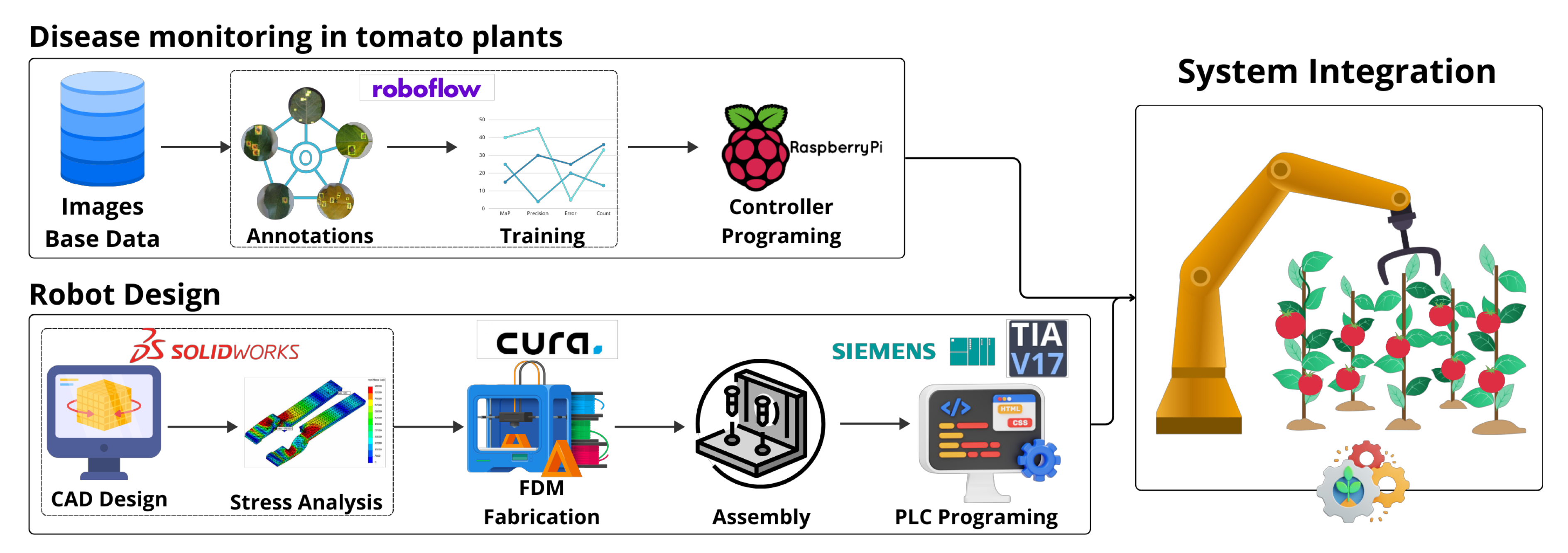
The Figure 2 details the proposed approach to develop a disease detection system in tomato plant leaves using a Deep Learning-based neural network. The Roboflow platform and the YOLOv5 architecture, known for its accuracy in object detection, were employed. This approach spans from data collection with images of affected leaves to real-time detection, including data preparation and preprocessing. Techniques such as normalization and data augmentation were applied to enhance the training set’s quality. The goal of this approach is to provide an efficient and accurate solution for the early identification of diseases, thus contributing to improving the health and performance of crops.
A. Collection of Data on Diseases in Tomato Plants - In the initial phase of the project, a data collection was carried out with the aim of building a representative dataset to investigate eight types of diseases in tomato plants, along with images of healthy plants. A total of 7,864 images were identified and gathered, providing a solid foundation for visually exploring and identifying tomato plant diseases. The collected diseases included Early and Late Blight, Leaf Mold, Mosaic Virus, Septoria Leaf Spot, Spider Mite Damage, and Yellow Leaf Curl. These diseases were selected for our project due to their high prevalence and impact on tomato leaves. These pathologies are known to adversely affect the health and productivity of tomato plants, posing significant challenges for farmers.
The Figure 3 displays representative images of diseased tomato leaves in the dataset, showcasing the diversity among the four diseases. Firstly, lesions caused by the same disease exhibit certain commonalities under similar natural conditions. Secondly, fruit spots in the early blight image can be easily confused with leaf spots. Finally, the damage in the leaf miner image is not very noticeable, which could pose a challenge for the neural network to detect accurately. The collected dataset possesses the following three characteristics: First, multiple diseases can coexist in the same diseased image. Second, most images contain complex backgrounds, ensuring a high performance of the approach in generalization. Finally, experts manually annotate all diseased images in the dataset.
B. Image Annotation - Image annotation is a vital step aimed at labeling the positions and classes of object spots in diseased images. For this stage, accurately annotating images in neural networks is essential to ensure the model’s training accuracy. Annotations provide key information about the objects and patterns present in the images, enabling the network to learn effectively and generalize to new data. Precise annotation facilitates the model’s ability to recognize and classify objects.
In Figure 4, you can observe how disease annotation is carried out in Roboflow. In this step, precise annotation of diseases must be done to avoid confusion for the neural network. The figure shows that only the region of interest is selected.
C. Training - Training images in a neural network involves feeding the network with a dataset of labeled images. During the process, the network adjusts its parameters by learning patterns and features present in the images. These adjustments occur through repeated iterations, where the network compares its predictions with the actual labels and adjusts its internal weights accordingly.
In Figure 5, the confusion matrix of a neural network specialized in detecting diseases in tomato leaves can be observed. This visual representation is crucial for evaluating the model’s performance, displaying true positives and negatives along the main diagonal, as well as false positives and negatives outside of it. Analyzing this matrix provides a detailed understanding of where the network makes errors, facilitating adjustments to enhance its accuracy, sensitivity, and specificity in detecting specific diseases in tomato leaves.
3.1.2. YOLOv5 Arquitecture
YOLOv5 belongs to the You Only Look Once (YOLO) series of computer vision models and is renowned for its robust object detection capabilities. Tailored for efficient feature extraction in images, YOLOv5 effectively tackles the task of simultaneously predicting bounding boxes and class labels within an end-to-end differentiable network. In the context of object detection, a scenario for which YOLOv5 is specifically crafted, the process entails extracting features from input images. Subsequently, these features undergo a prediction system to delineate bounding boxes around objects and forecast their respective classes.
The YOLO model pioneered the integration of predicting bounding boxes and class labels within a seamless, end-to-end differentiable network. This groundbreaking approach has set the standard in object detection methodologies.
The YOLO network comprises three essential components, as illustrated in Figure 5, each playing a crucial role in its comprehensive functionality:
- Backbone - This is a convolutional neural network designed to aggregate and generate image features at various granularities. It forms the foundation for extracting meaningful information from input images.
- Neck - Comprising a series of layers, the neck is responsible for blending and amalgamating image features. Its role is crucial in preparing these features for subsequent prediction steps.
- Head - Taking input features from the neck, the head component executes the final steps of the process. It is responsible for making predictions related to bounding boxes and class labels, thus completing the object detection pipeline.
3.1.3. YOLO Training Procedures.
The methodologies employed during the training phase significantly impact the ultimate performance of an object detection system, yet these crucial steps are often overlooked in discussions. Let’s delve into two key training procedures integral to YOLOv5, shedding light on their importance and additional details:
- Data Argumentation - This crucial step involves applying transformations to the foundational training data, expanding the model’s exposure to a broader spectrum of semantic variations beyond the isolated training set. By incorporating diverse transformations such as rotation, scaling, and flipping, data augmentation enhances the model’s robustness and adaptability to real-world scenarios.
- Loss Calculations - YOLOv5 employs a comprehensive approach to loss calculations, considering the Generalized Intersection over Union (GIoU), objectness (obj), and class losses. These loss functions are meticulously crafted to construct a total loss function. The objective is to maximize the mean average precision, a key metric in assessing the model’s precision-recall performance. Understanding and fine-tuning these loss functions contribute significantly to optimizing the model’s accuracy and predictive capabilities.
3.1.4. Data Augmentation in YOLOv5.
During each training batch, YOLOv5 utilizes a data loader to process training data, incorporating online data augmentation. This dynamic process involves three distinct types of augmentations:
- Scaling - Adjustments in scale are applied to the training images, enabling the model to adapt to variations in object sizes and spatial relationships.
- Color Space Adjustments - Alterations in the color space of the images contribute to the model’s ability to generalize across different lighting conditions and color distributions.
- Mosaic Argumentation - A particularly innovative technique employed by YOLOv5 is mosaic data augmentation. In this approach, four images are combined into four tiles of random ratios. This method not only diversifies the training dataset but also challenges the model to comprehend and analyze complex scenes where multiple objects interact within a single image.
The mosaic data augmentation technique stands out as a unique and effective strategy to enhance the model’s robustness and performance across diverse scenarios. By exposing the model to a more comprehensive range of training instances, YOLOv5 aims to improve its adaptability and accuracy in real-world applications.
3.1.5. CSP Backbone (Cross Stage Partial).
Both YOLOv4 and YOLOv5 incorporate the CSP Bottleneck for formulating image features. The inclusion of the Cross Stage Partial (CSP) module effectively addresses duplicate gradient challenges present in larger Convolutional Neural Network (ConvNet) backbones. This not only results in fewer parameters but also reduces Floating Point Operations Per Second (FLOPS), enhancing computational efficiency without compromising performance. This is particularly crucial within the YOLO family, where inference speed and compact model size hold paramount significance. The CSP models draw inspiration from DenseNet, a foundational architecture designed to interconnect layers in ConvNets.
3.1.6. PA-Net Neck.
Both YOLOv4 and YOLOv5 implement the PA-NET neck for feature aggregation. In the context of detection necks, the authors of EfficientDet identified BiFPN as the optimal choice, presenting a potential area for YOLOv4 and YOLOv5 to explore further with alternative implementations. This exploration could lead to advancements in the efficiency and performance of their architectures.
It is noteworthy that YOLOv5 draws on research insights from YOLOv4 in determining the most suitable neck for its architecture. YOLOv4 extensively investigated various possibilities for the optimal YOLO neck, including:
- FPN - (Feature Pyramid Network): A pyramid-shaped hierarchical architecture for multi-scale feature representation.
- PAN -(Path Aggregation Network): Focused on aggregating features from different network paths to enhance information flow.
- NAS-FPN - (Neural Architecture Search - Feature Pyramid Network): Involves employing neural architecture search techniques to optimize the feature pyramid network.
- BiFPN - (Bi-directional Feature Pyramid Network): A bidirectional approach to feature pyramid networks, promoting effective information exchange.
- ASFF - (Adaptive Spatial Feature Fusion): A mechanism for adaptively fusing spatial features to enhance object detection capabilities.
- SFAM - (Selective Feature Aggregation Module): A module designed for selectively aggregating features to improve the model’s discriminative power.
In conclusion the initial launch of YOLOv5 showcases impressive speed, performance, and user-friendly features. While YOLOv5 doesn’t introduce groundbreaking architectural advancements to the YOLO model family, it does bring forth a novel PyTorch-based training and deployment framework. This framework represents a significant enhancement in the realm of object detectors, pushing the boundaries of the state of the art in terms of training efficiency and deployment effectiveness.
3.1.7. PILOT EXPERIMENT
In the initial pilot phase, a dataset comprising 1950 images was employed to preliminarily assess the performance of the neural network. These images were carefully selected with the purpose of providing a first impression of detection accuracy. In this initial sample, the model achieved an accuracy of 64.2, and an mAP of 56.1 was recorded, as shown in Figure 5(b), an essential metric in the evaluation of object detection models based on Deep Learning. Although these results offer an initial overview of the model’s effectiveness, it is highlighted that, in the final test with a more extensive set of 7864 images, a notable improvement was achieved with an accuracy of 90.2 and an mAP of 92.3, as shown in Figure 5(a). This evolution underscores the importance of iteration and continuous improvement, recognizing the need to expand the dataset and refine the neural network to achieve even higher levels of accuracy in disease detection across a more diverse and representative set of images.
3.1.8. Validity and Reproducibility
- It can be mentioned that the study presents a clear and detailed methodology for detecting plant diseases using deep transfer learning. The methods used seem to align with the study’s objective and are described with enough detail to allow study replication. However, there is no information on the validity of the data used in the study, which could impact the results. In general, more information is required to fully assess reproducibility and validity [38].
- The suggested model is addressed using data augmentation methods and capturing images in different environments and conditions. Reproducibility and validity are addressed through data augmentation techniques, careful selection of image data, and evaluation methods such as confusion matrices. However, it does not explicitly provide specific reproducibility algorithms or codes [35].
- A detailed description of the proposal and the experimental design used is provided, indicating measures taken to ensure the internal and external validity of the study. Sufficient details about the study proposal and the experimental design are given to enable other researchers to reproduce it. Simulation and experiment results are also presented, and both can be replicated using the same manipulator robot and experimental setup. Overall, while the study presents promising results, further research is needed to confirm the effectiveness of the proposal and assess its applicability in various contexts [39].
The three provided research studies bolster and validate the current project centered on the development of a neural network for the detection of diseases in tomato plants. The dedicated focus on reproducibility, the implementation of data augmentation methods, and the detailed description of experimental designs in the mentioned studies support the robustness of the methodology employed in the current project.
3.2. Robotic Arm Design and Manufacturing
For the development of the robotic arm prototype, the main challenge was the extension of the robot to adapt its height with two prismatic axes. We mainly used SolidWorks CAD software for the development of parts and necessary analysis for the final development of the robot arm prototype, and Autodesk Fusion 360 as support software for some parts. The final prototype has 5 rotational axes and 2 prismatic ones, for a total of 7 DOG, which will give it vast mobility to reach complex positions for its final use.
3.2.1. Cad Design
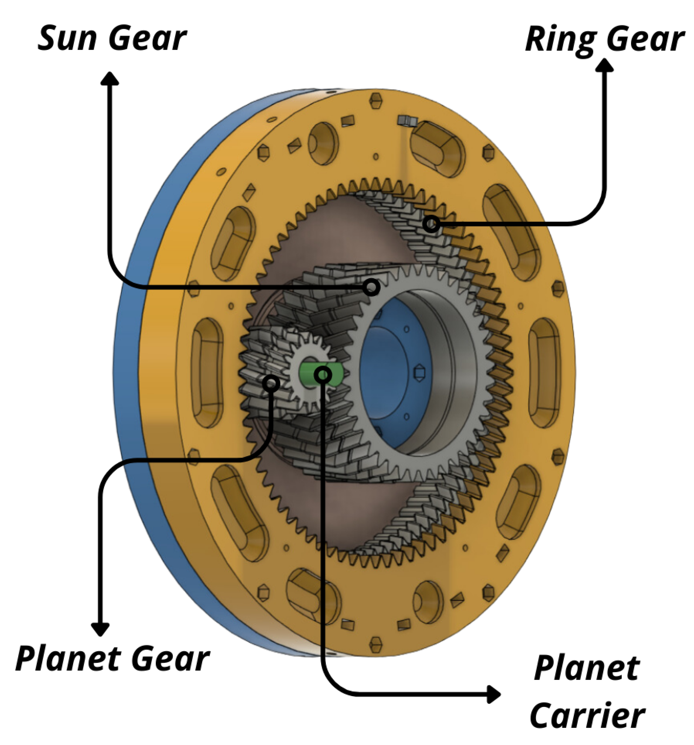
Rotational Actuators - In the first design stage, the rotational actuators are fundamental for the robot movements, on which it have a planetary gears mechanism as shown in the Figure 6, of which it has three different sizes. The actuators contain a gear ratio corresponding to their size: The large actuator is 1:108, the medium actuator is 1:76.5, and the small actuator is 1:64.4.
Figure 7.
Rotational Actuator - Internal view of the planetary gear mechanism.
The rotational actuators provide movement in degrees as a measurement unit on all five rotational axes. Each one has a rotational displacement of less than 360 degrees of movement in order not to exceed the limits proposed in the final design of the robot body.
Planetary gear transmission ratio formula, The following nomenclature will be used:
- Tr: Ring gear spin speed
- Ts: Planet spin speed
- Ty: Planet carrier spin speed
- R: Ring gear teeth
- S: Suns’s teeth
- S: Planet’s teeth
Prismatic Actuators - In the second stage, which contemplates the prismatic extension mechanism, the mechanism consists of two parts, the first with a NEMA 17 stepper motor coupled to the lower part, which is fixed and has as an axis a worm screw of 8mm in diameter and 60mm long that connects to a trapezoidal nut that is coupled to the second moving physical part that performs the extension movement through the travel of the nut by the worm screw. Included in the model are 4 smooth rods of 8mm thick in the 4 corners of the model to give rigidity and stability to the robot.
Figure 8.
Prismatic Actuator - Mechanism View.
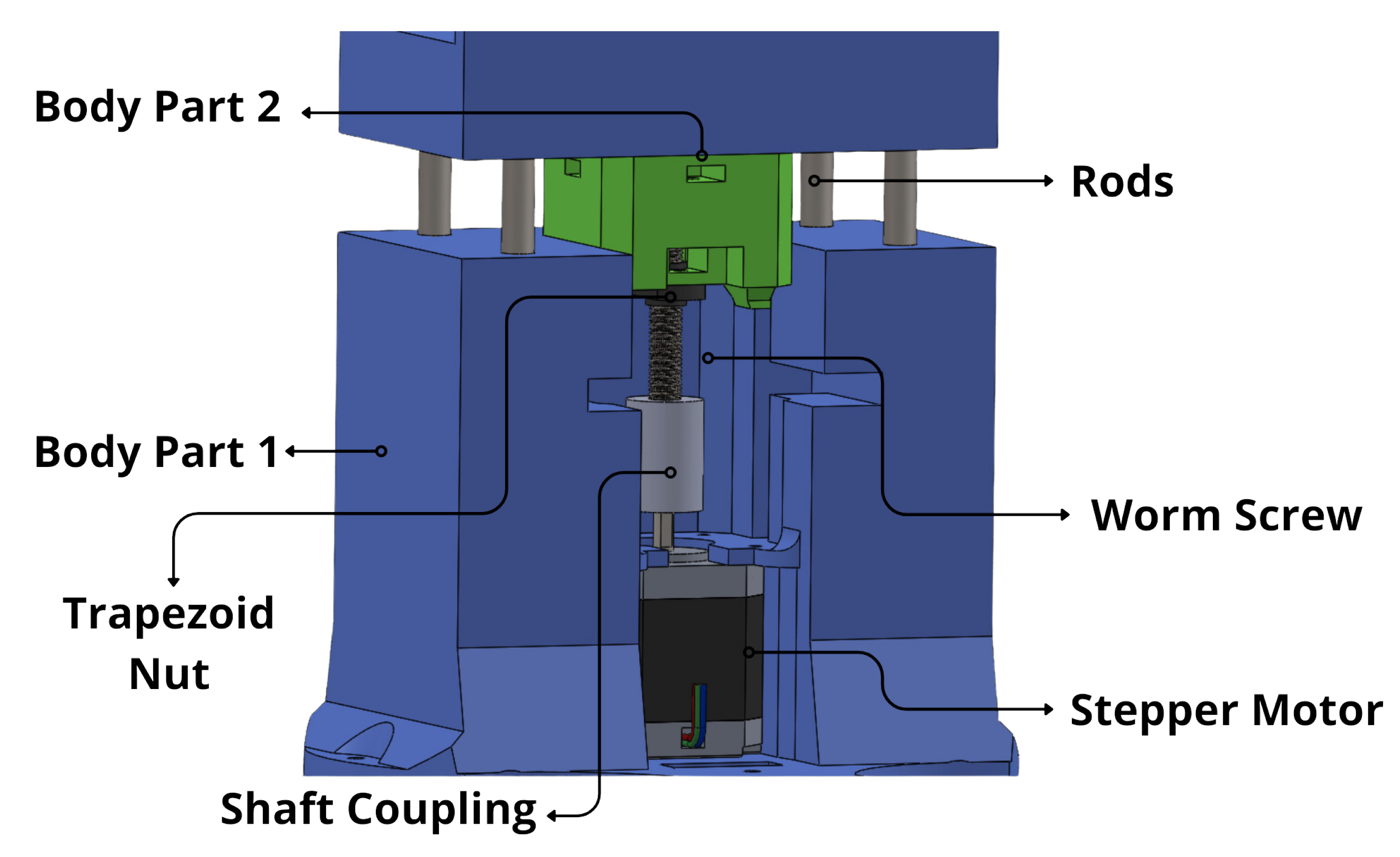
The prismatic extension mechanism will be included in two segments of the robot; the first prismatic axis will be included between rotational axis one and rotational axis two, providing a maximum extension of 24mm in length. The second prismatic axis will be included between rotational axis two and rotational axis three; this will provide a maximum extension of 16.5mm in length. As a final extension, the two prismatic extension mechanisms will provide a total of 40.5mm of final total extension to the robotic model.
The drivePower (P) of a screw worm is made up of the sum of three main components, as reflected in the following expression:
in which…
- PH Is the power required to move the material horizontally.
- PN is the power required to drive the screw in freewheeling operation.
- Pi is the power required for the case of an inclined worm screw.
- Q is the flow of transported material, in t/h
- H is the height of the installation, in m
- D is the diameter of the link section of the conveyor casing, in m
- C0 is the resistance coefficient of the transported material.
The total Power (P) required to drive a screw link is the sum of the various power requirement, as a final result shown in the equation:
Which finally can be expressed as...
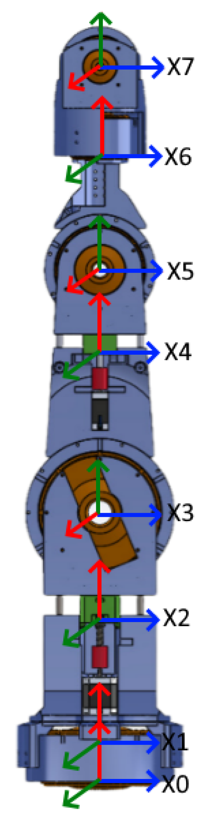
Final Robot Design - Once the rotational and prismatic mechanisms are calculated, we can take the necessary measurements of the actuators to create the body or housing of the robot, which has five rotational actuators, two prismatic mechanisms, and three links that connect to each other. Each of the parts of the robot’s housing was designed thoroughly in CAD SolidWorks parametrically to obtain the best possible design results and was also accompanied by motion and load studies to observe the kinematics and efficiency of the robot.
Figure 9.
Final Design.
3.2.2. Motion and Stress Analysis
Motion Analysis - The final robotic model was submitted to a motion study to be analyzed with a simulation involving all its segments and actuators working in a constant movement routine, and the final assembly robotic model was analyzed. The motion study is needed to simulate real-time conditions that can have an effect on its kinematics; elements such as gravity, contact forces, weight, inertia, torque, energy consumption, velocity, acceleration, angular velocity, and linear displacement were included in this study. It is necessary to use this procedure to verify and rectify elements that can affect the functionality of the model in real-life situations.
Figure 10.
Motion Analysis - Position 1.
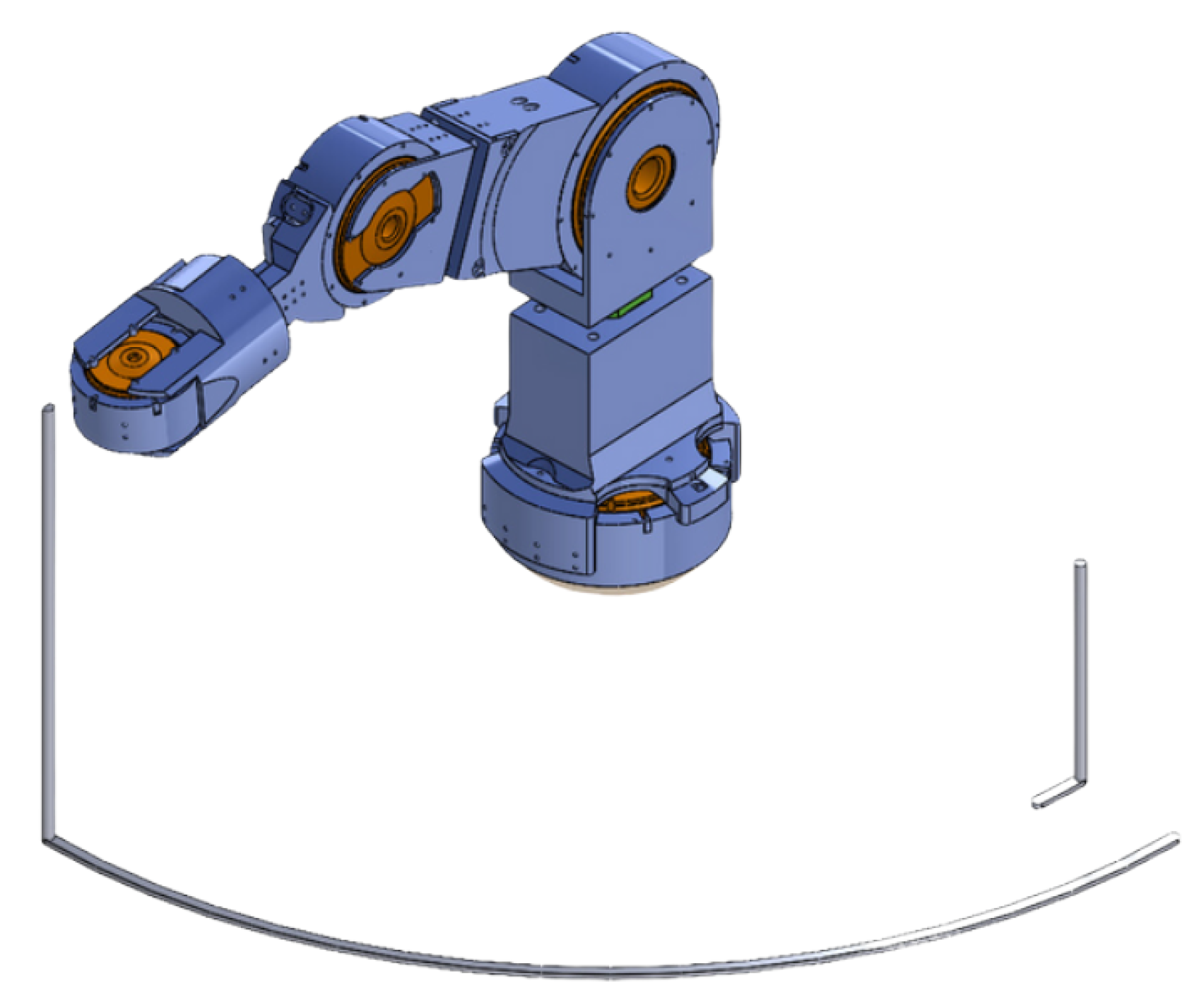
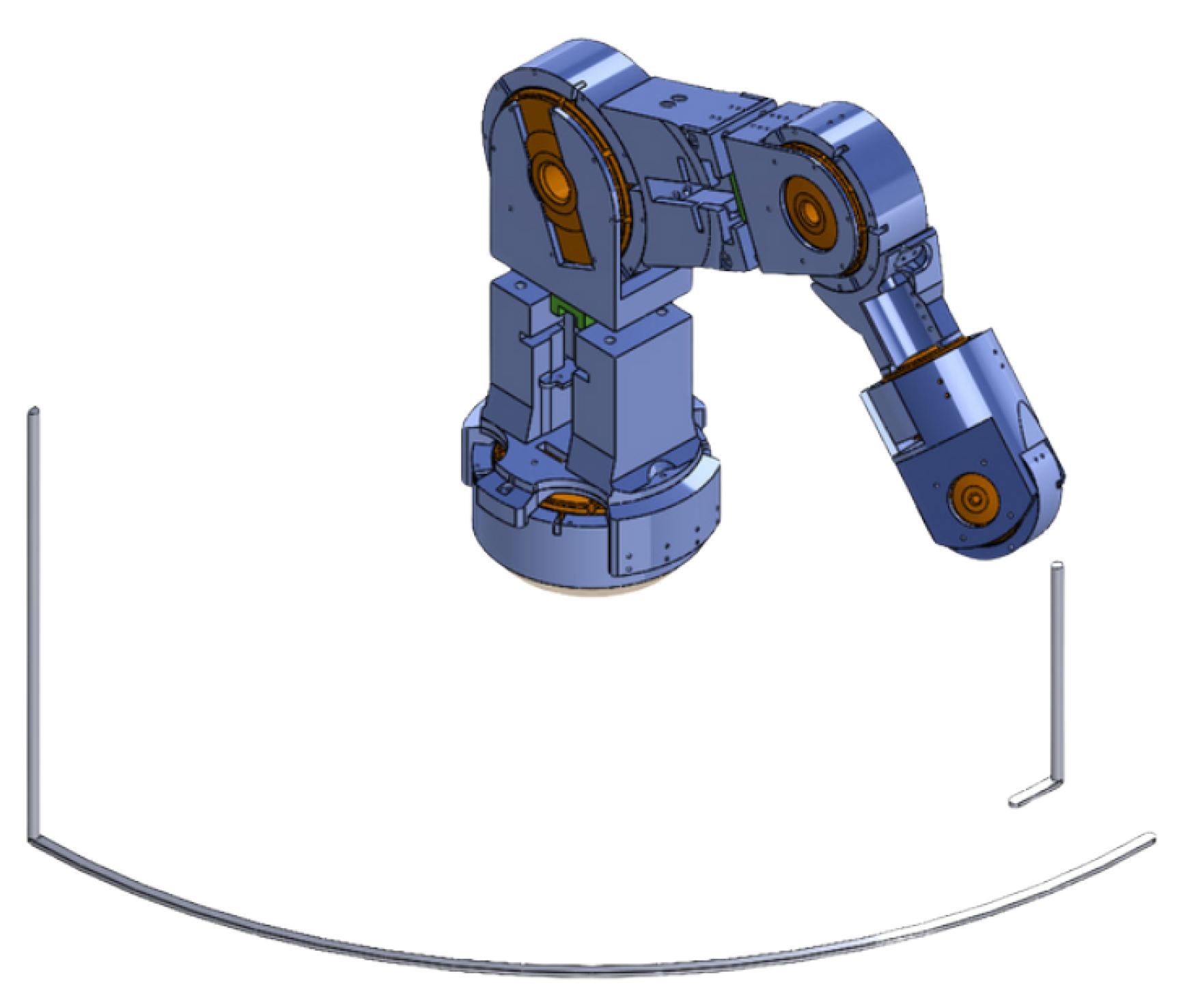
Figure 11.
Motion Analysis - Position 2.
Stress Analysis - A stress study was performed to verify the deformation that can be generated by high loads applied to the robot. As well also get the factor of safety in each of the pieces, since for its fabrication will be used ABS type plastic which is lighter but less rigid. Stresses and displacements were the study approach given to each of the pieces in order to obtain a good safety factor in the final model of the robot body and to avoid accidents or breakage of the material used to manufacture each of the pieces.
The simulation included all actuators working together to reach two specific positions and returning to their initial positions to obtain the results and get to know all the information needed to proceed with a verification of the pieces or, in the best case possible, to proceed to the next step.
Figure 12.
Stress Analysis - Displacements.
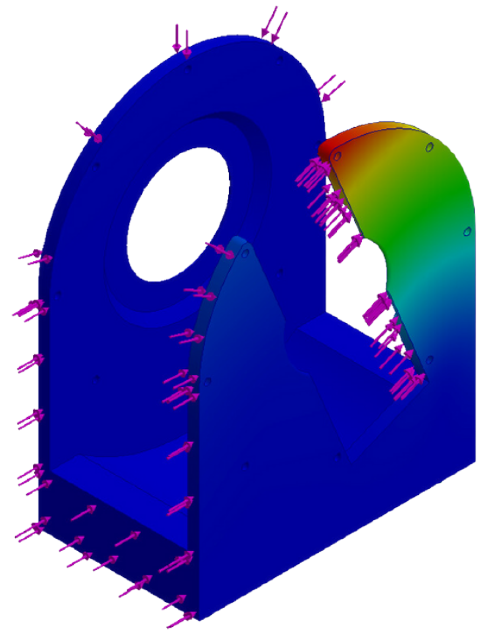
The safety factor should be greater than 1, since the higher the value, taking 1 as the starting point, the better the resistance to stress that the part will have under working conditions. On the other hand, if the safety value is less than or equal to 1, it is an indication that the structure will fail immediately upon reaching the stress applied to it in the study.
To find the Factor of Safety(FOS) , is necesary to used the following expression:
3.2.3. FDM Fabrication
The FDM process, which stands for "Fuse Deposition Modeling", better known as 3D printing, was used to manufacture the robot model. Two Creality Ender 3D printers were used, specifically the Ender 3 V2 and Ender 3 S1 models. The manufacturing material used was ABS for its physical properties, resistance to high temperatures, and greater rigidity.
To manufacture each of the parts, the following steps were followed:
- Step 1: Convert each of the CAD files individually to an STL extension format.
- Step 2: Obtain the 3D processing software CURA and install it on a PC, the version used for the fabrication of the parts was CURA 5.3.0.
- Step 3: Configuration in the software of each printer that will be used to manufacture the parts.
-
Step 4: General parameterization. In software, there are several configurations that the user can modify to his preference. For our parts manufacturing on both printers, we will use the same print settings profile except for the following parameters:- Layer height: When the parts to be manufactured are very small, it is required to have a layer height between 0.15mm and 0.10mm in order not to lose the shape and quality of the parts, and the larger the part, the less impact the layer height will have. A general recommended value would be a height greater than or equal to 0.2mm. The lower the value, the longer it will take the machine to manufacture the parts.- Number of external walls: This value is the number of external walls that the machine will make before starting with the shell-like filling; these walls provide rigidity to the torsion and therefore a better final finish where you do not get to see the inner filling pattern.- Infill: This parameter is the one that provides most of the rigidity to the parts and also the one that consumes the largest amount of manufacturing material, depending on the filling pattern applied to the parts.In the model, a percentage between 20 and 40 infill percentage was used in the parts in variation to their function and size. Pieces that perform mechanical work and undergo greater stress were given more infill.- Horizontal expansion: For this configuration, a test must be performed depending on the material; in this case, ABS was used. For this test, a cube measuring 20 x 20 x 20mm is made in order to measure if it has undergone an expansion or if the material is compressed. This happens due to temperature variations at the time of extruding the material through the nozzle of the printing machine and external conditions such as ambient temperature. Once the test is done, we proceed to measure with a vernier or a micrometer and see how much variation there is from the original measurements.In the test, it was verified that the material used expanded by 0.12 mm, and a parameter of -0.12 was applied to counteract this excess material.
-
Step 5: Prepare each piece in the CURA software. Once all the above is configured, each piece is added individually and processed in the software, giving us the weight data in grams and the printing time.Click on the save option, and the program will automatically generate a G-CODE file that must be saved on a microSD memory card.
- Step 6: Level the printer’s print bed manually.
- Step 7: Start printing each of the parts.
3.2.4. Robot Controller – PLC Programming
The controller is one of the most important elements in the robot, since without it we would not have any control over the electrical elements such as the motors, which are an essential element for the operation of the robot.
Two Siemens PLC controllers are used:
- SIMATIC S7-1200, CPU 1214 DC/DC/DC with firmware version 4.2
- SIMATIC S7-1200, CPU 1212 DC/DC/DC with firmware version 4.2
The reason why two controllers were used is because of the Pulse Train Output (TPO) physical outputs, which consume two physical outputs of the controller: the first output is the pulse train, and the second output defines the direction. The CPU 1214 controller contains 4 configurations of type TPO, which consumes all its physical outputs with this configuration, and the second controller, CPU 1212, contains only 3 configurations of type TPO, which consumes all its outputs as the previous one. In order to make use of these TPO-type outputs, drivers capable of processing these signals at a voltage of 24 volts DC are needed.
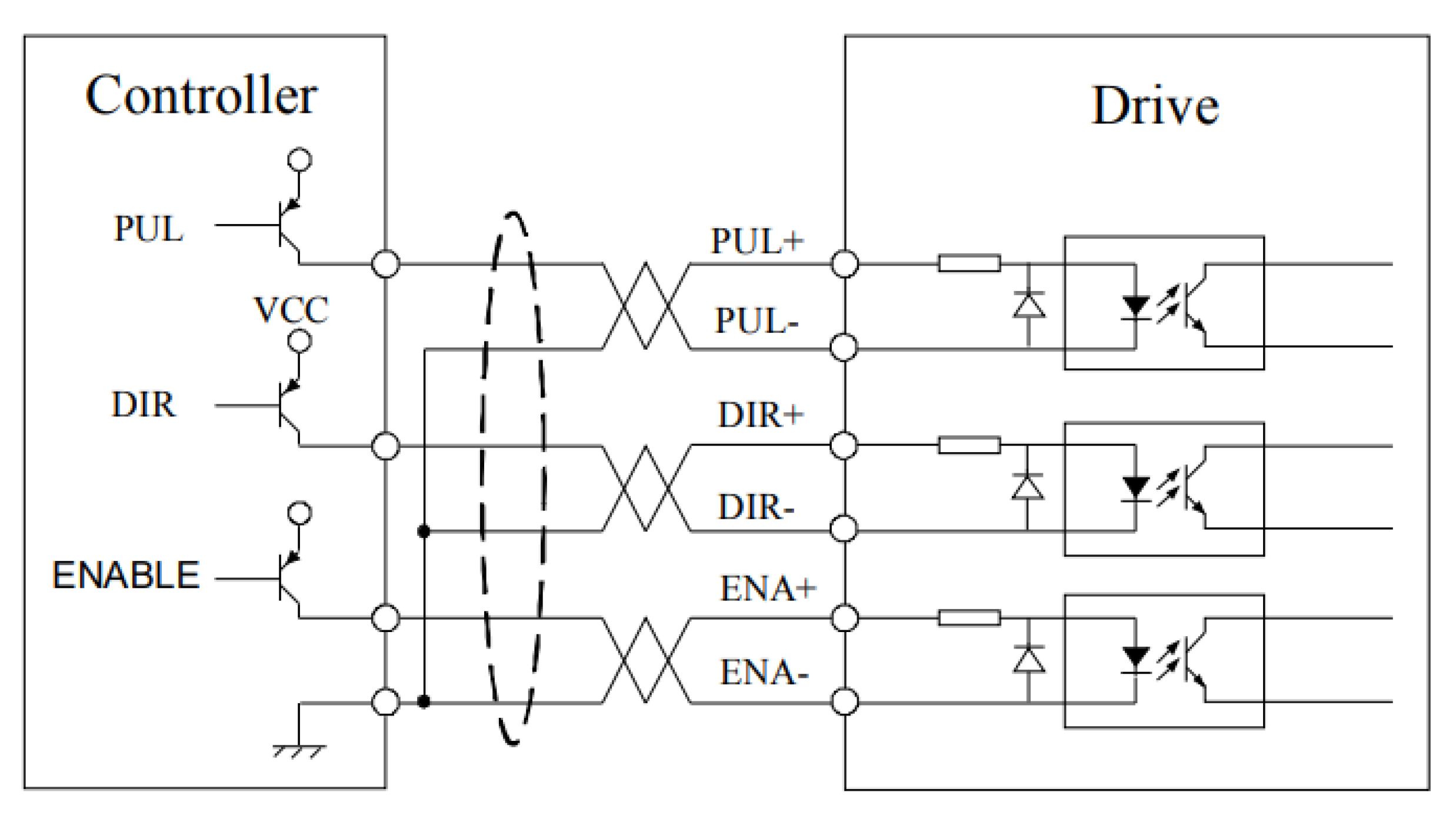
The controller used to receive the TPO signals and control the Nema 17 bipolar stepper motors is a DM542, which is capable of withstanding voltages between 20V and 50V DC and a maximum current consumption by the motor of 4.2A. We will work with PNP-type signals at all times, and as common between the PLC and drivers is the neutral signal and 24V signals.
Figure 13.
Connection diagram between the controller and DM542 driver - PNP connection.
Tia Portal V17 is the software used to program Siemens PLCs. In the program that was created, were added the two PLC controllers S7-1200, a HMI display KTP700 Basic panel to manipulate certain parameters manually, and an expansion module SM1223 to have auxiliary digital inputs and outputs. Each of these elements, except for the module, will have a unique IP to communicate the two PLCs in the same network segment.
For the communication, the Profinet S7-communication protocol PUT/GET, an exclusive communication protocol for the Siemens S7 range, was used to facilitate the communication between the two PLCs. The PLC S7-1214 will be the main controller where all the control logic of the robot is programmed, which will include manual control, automatic routine control, total reset of the program, home positioning of the robot, and other functionalities that will be controlled from the HMI KTP700 screen with a friendly user interface for an operator.
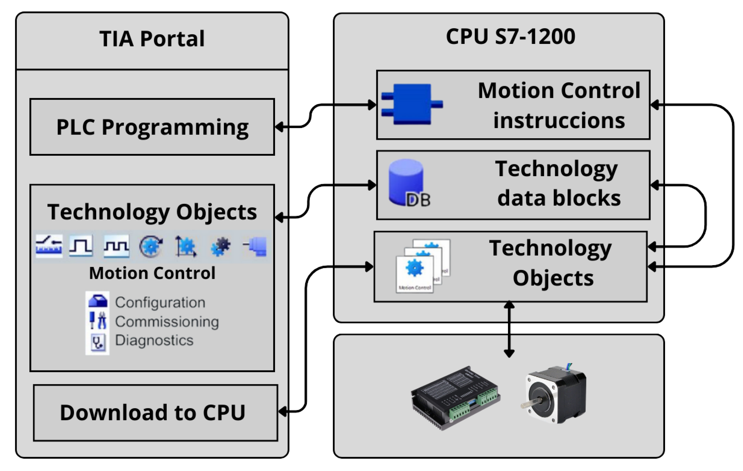
The most important thing in the programming is the configuration of the TPO outputs. For this, in the PLC configuration section, the Technology Objects block is used. Here is where it is adjusted with the desired parameters, such as the number of pulses that it will send to the DM542 driver that we will synchronize physically separately to the same value that is set up in the PLC configuration, for which it is selected the amount of 6400 steps/rev for all motors, and other parameters that are adjusted according to the model of the robot. Once the technology object block is configured, make use of motion control instructions such as speed, halt, reset, jog control, and absolute movements, and set it to home. That same configuration process is applied in the PLC 1212 to control the outputs that will give movement to the three final motors. The PLC 1214 will use the PUT and GET blocks to be able to write and read data in the PLC 1212. 4 bytes of data will be used in each block to have a vast amount of data and to control each one effectively.
The GET block is in charge of reading data from the PLC 1212 and storing it in a bit or mark to be able to make use of it in the general configuration.
The PUT block is in charge of writing data from the PLC 1214 to the PLC 1212. And thus to be able to control the variables from the main controller with the interface created to manipulate the movements of the robot.
Figure 14.
General hardware/software control diagram.
4. Results
4.1. Neural Network
In this section, key results obtained through the implementation of the neural network will be presented, emphasizing fundamental metrics such as accuracy, mAP (Mean Average Precision), and real-time detection capability. These outcomes will provide a detailed overview of the network’s performance in plant disease detection.
4.1.1. Precision and mAP
In the initial phase, a pilot test was carried out to see how the neural network could develop with 25 percent of the images from the data-set of tomato plant diseases, a data-set consisting of 1950 images was employed for a preliminary assessment of the neural network’s performance. These images were meticulously selected to provide an initial evaluation of accuracy in plant disease detection. In this initial sample, the model exhibited an accuracy of 64.2 percent, with a recorded mAP of 56.1 percent, as evidenced in Figure 15(b), a critical metric for assessing deep learning-based detection models. While these results offer an initial insight into the model’s effectiveness, it is crucial to highlight that in the final test with a more extensive set of 7864 images, a significant improvement was achieved, reaching an accuracy of 90.2 percent and an mAP of 92.3 percent, as presented in Figure 15(a). This progress emphasizes the importance of iteration and continuous improvement, recognizing the need to expand the data set and refine the neural network to achieve even higher levels of accuracy in disease detection, encompassing a more diverse and representative spectrum of images.
The achievement of accuracy in the neural network was not only supported by the expansion of the dataset but also by the constant adaptation of the network. The results clearly demonstrated that iteration and continuous optimization are crucial elements for advancing towards higher accuracy levels. The transition from an initial accuracy of 64.2 percent to an outstanding 90.2 percent like is shown in Figure 16 highlights the neural network’s ability to learn and improve when exposed to a more extensive variety of data. This process underscores the need for a development strategy that includes adaptability and constant evolution, ensuring that the model can successfully handle diverse scenarios and guarantee accurate detection across a broad range of conditions and environments.
4.1.2. Disease Accuracy
Figure 17 provides a detailed perspective on the accuracy achieved for each analyzed disease, encompassing a representative set of the most common conditions in tomato plantations. During the evaluation, a total of 14,192 annotations were made, approximately 2 annotations per image, contributing to a comprehensive analysis of various pathology’s. Among the considered diseases, Early Blight stands out, a fungal infection that mainly affects plant leaves. The model achieved an accuracy of 87 percent, supported by 1295 annotations, demonstrating robust performance in identifying this common disease.
In the case of Late Blight, a disease caused by the oomycete Phytophthora infestans, an outstanding accuracy of 91 percent was attained, supported by 1562 annotations. This result suggests substantial efficacy in accurately identifying this disease, which can be devastating for tomato crops. The Tomato Leaf Miner, an insect that burrows into plant leaves, and Septoria Leaf Spot, characterized by mold development on leaves, both presented equally high accuracy of 97 percent, with 961 and 1945 annotations respectively, highlighting the model’s ability to efficiently address diverse pathology’s affecting tomato plant health.
Despite Mosaic Virus, a viral disease affecting normal plant development, recording a slightly lower accuracy compared to other diseases, it maintained adequate detection efficiency at 86 percent. Septoria Leaf Spot, a fungal infection causing lesions on leaves, exhibited an accuracy of 91 percent. On the other hand, Spider Mite Damage, commonly associated with mites, surprised with an exceptional accuracy of 99 percent. Finally, Yellow Leaf Curl, a disease affecting leaf development, achieved an accuracy of 94 percent, consolidating strong performance in identifying these specific diseases. These results reveal the neural network’s ability to accurately distinguish among the various individually assessed pathologies, emphasizing the potential for further improving accuracy rates in future model iterations.
In Figure 18, eight diseases are detected in the crop, each with distinct characteristics. Early Blight, caused by Alternaria solani, results in dark, concentric lesions on leaves, leading to premature defoliation. Late Blight, induced by Phytophthora infestans, poses a threat to potato and tomato crops with water-soaked lesions. Leaf Miner, caused by larvae of various insects, creates tunnel patterns on leaves, potentially weakening the plant. Leaf Mold, from the fungus Fulvia fulva, causes yellowish or brownish patches on tomato leaves, compromising plant health. Mosaic diseases, viral infections with mosaic-like leaf patterns, disrupt photosynthesis and stunt growth. Septoria Spot, by Septoria lycopersici, leads to small, dark spots on tomato leaves, risking defoliation. Spider Mites, arachnids feeding on plant sap, cause stippling and leaf discoloration. Yellow Curl, associated with viral infections transmitted by whiteflies, results in yellowing and curling of leaves, hindering photosynthesis.
4.1.3. Real-Time Detection
In Figure 19, we present a compelling demonstration of the real-time detection capabilities of our neural network designed for the diagnosis of tomato plant diseases. The two sets of images, denoted as Figure 19(A), depict instances of tomato plants afflicted with Yellow Leaf Curl, while the subsequent images, labeled as Figure 19(B), showcase plants suffering from Leaf Mold. This visual representation serves as a testament to the effectiveness and accuracy of our neural network in identifying and distinguishing between different diseases in the tomato plant domain.
The initial pair of Figure 19(a) vividly illustrate the characteristic symptoms of Yellow Leaf Curl, a prevalent and economically significant disease affecting tomato crops. The intricate neural network architecture seamlessly captures the distinct visual cues associated with this malady, enabling precise and real-time identification. Subsequently, the following set of Figure 19(b) portrays tomato plants grappling with the challenges posed by Leaf Mold. The neural network successfully discerns the subtle nuances and unique patterns indicative of this specific disease, further highlighting the robustness of our detection model.
These real-time detections exemplify the practical application of our neural network in the field of precision agriculture. By swiftly and accurately identifying plant diseases, our technology empowers farmers with timely information, enabling proactive measures to mitigate the impact on crop yield. The integration of artificial intelligence in agricultural practices continues to be a pivotal step toward sustainable and efficient farming methodologies.
4.2. End Effector
Throughout the project, a significant achievement has been reached with the realization of the manufacturing of an end effector through 3D printing, utilizing PLA as the base material. This effector is characterized not only by its mechanical efficiency but also by its contemporary and innovative design. The incorporation of a Raspberry Pi 4 into its structure adds an additional level of sophistication, allowing for the implementation of a neural network.
Next, Figure 20 is presented, providing a visual representation of the final result of this collaborative effort. In this image, the 3D-printed effector can be appreciated with its modern style, along with the strategic integration of a camera at the top. The crucial function of this camera, as evidenced in Figure 20, is to facilitate real-time detection. The combination of the Raspberry Pi 4 and the camera provides advanced capabilities for data processing and analysis, opening new perspectives for applications that demand precision and adaptability in dynamic environments.
4.3. Motion Analysis
For the motion analysis, a parameter study was done in two different stages. The first motion study was performed with the un-extended prismatic actuators to obtain data about power consumption, torque, angular velocity, acceleration at the robot tip, and displacement at the robot tip. These parameters are shared regardless of the state of the prismatic actuators. In the second study, the same parameters were analyzed, but now including linear velocity and force, since these are the parameters that are applied in the motors coupled to the prismatic actuators.
In the following graphs, you can see the data variation generated by the activation of the prismatic actuators and the effects caused by obtaining a greater height for the robot.
The power consumption represented in Figure 20 had effects due to the extension of the prismatic axes when generating a new height position. The consumption without the extended prismatic axes was up to 0.09 watts as a maximum value, but when generating the prismatic extension, the consumption went up to a maximum of 5 watts as a maximum value, specifically in motor number two, which is related to the shoulder of the robot.
The torque graphs shown in Figure 21 recorded values that generated quite a difference between the two instances being compared. Motors two and three are the ones that generate the most torque due to their function as the robot’s shoulder and elbow. The results in the non-extension position gave us a maximum value of 151 N-mm in motor 2, and in motor 3, a maximum of 62 N-mm. The torque with the axes in extension position in the above-mentioned motors increased from 151 N-mm to 9471 N-mm in motor two and from 62 N-mm to 2295 N-mm in motor three. Motors one and four obtained a maximum change range of 13 N-mm, and in motor five, the torque remained the same in both positions.
The angular velocity shown in Figure 22 did not show changes in any of the two scenarios; it remained the same in both studies, providing completely identical graphs. The maximum speed reached was 68 deg/sec in motor four and a minimum of 28 deg/sec in motor five.
Figure 23.
Rotational actuators: Angular velocity comparison graphs. Motor 1 shown on graphs a and b. Motor 2 shown on graphs c and d. Motor 3 shown on graphs e and f. Motor 4 shown on graphs g and h. Motor 5 shown on graphs i and j.
Figure 23.
Rotational actuators: Angular velocity comparison graphs. Motor 1 shown on graphs a and b. Motor 2 shown on graphs c and d. Motor 3 shown on graphs e and f. Motor 4 shown on graphs g and h. Motor 5 shown on graphs i and j.
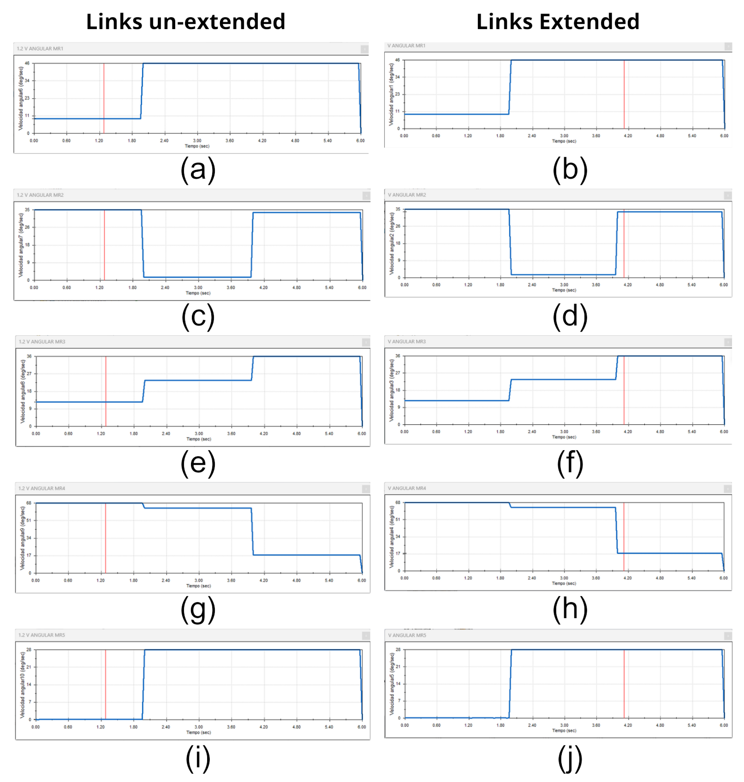
Figure 24.
Prismatic actuators: Power consumption, force and velocity graphs.
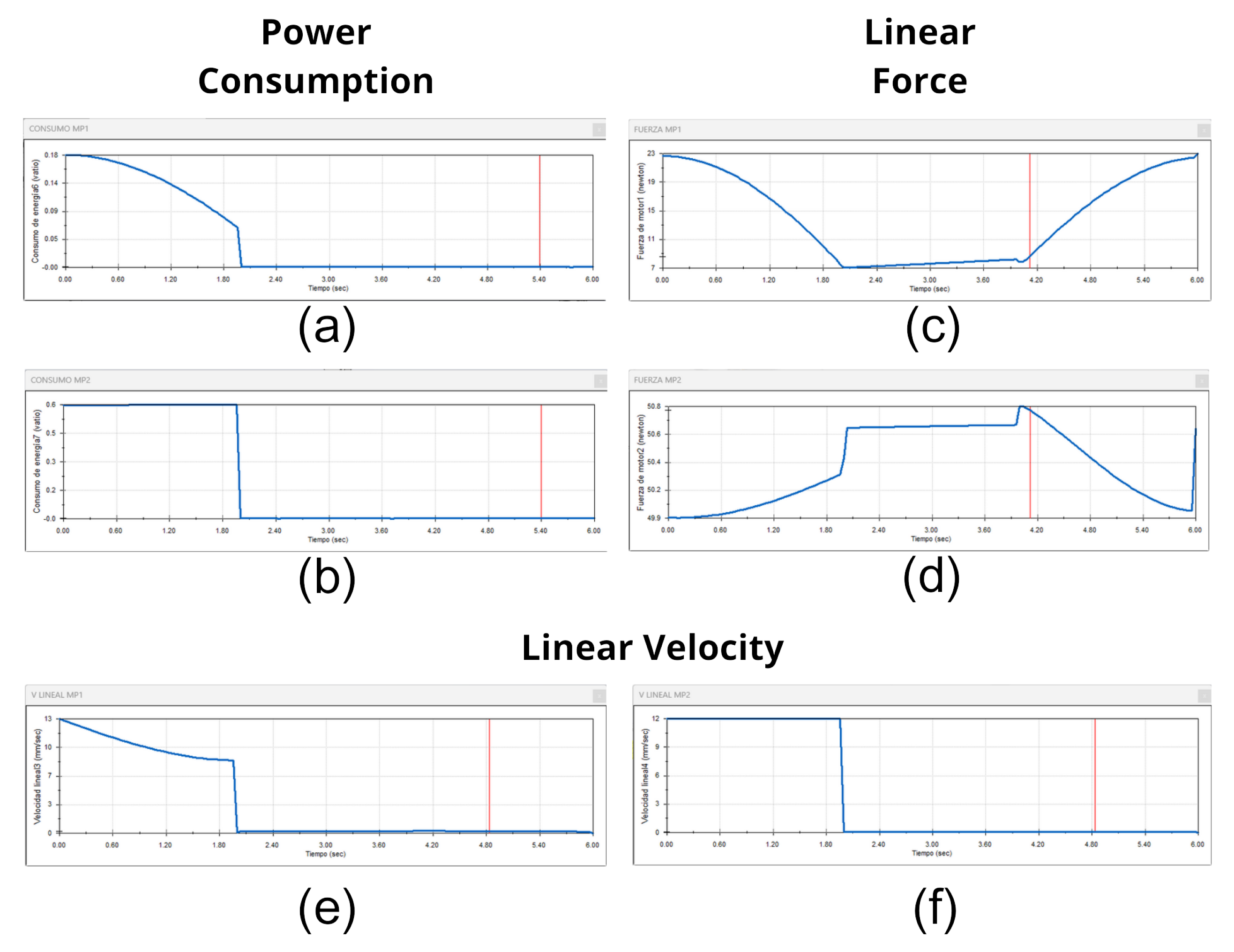
The motors corresponding to the prismatic extension mechanism provided fairly stable data. The consumption of both motors was at a maximum of 0.60 watts and a minimum of 0.18 watts. The linear force exerted to extend the robot links gave a maximum force of 50.8 Newtons and a minimum force of 23 Newtons. And its linear velocity was almost the same, with a maximum of 13 mm/sec and a minimum of 12 mm/sec.
Figure 25.
Prismatic actuators: Acceleration and displacement.
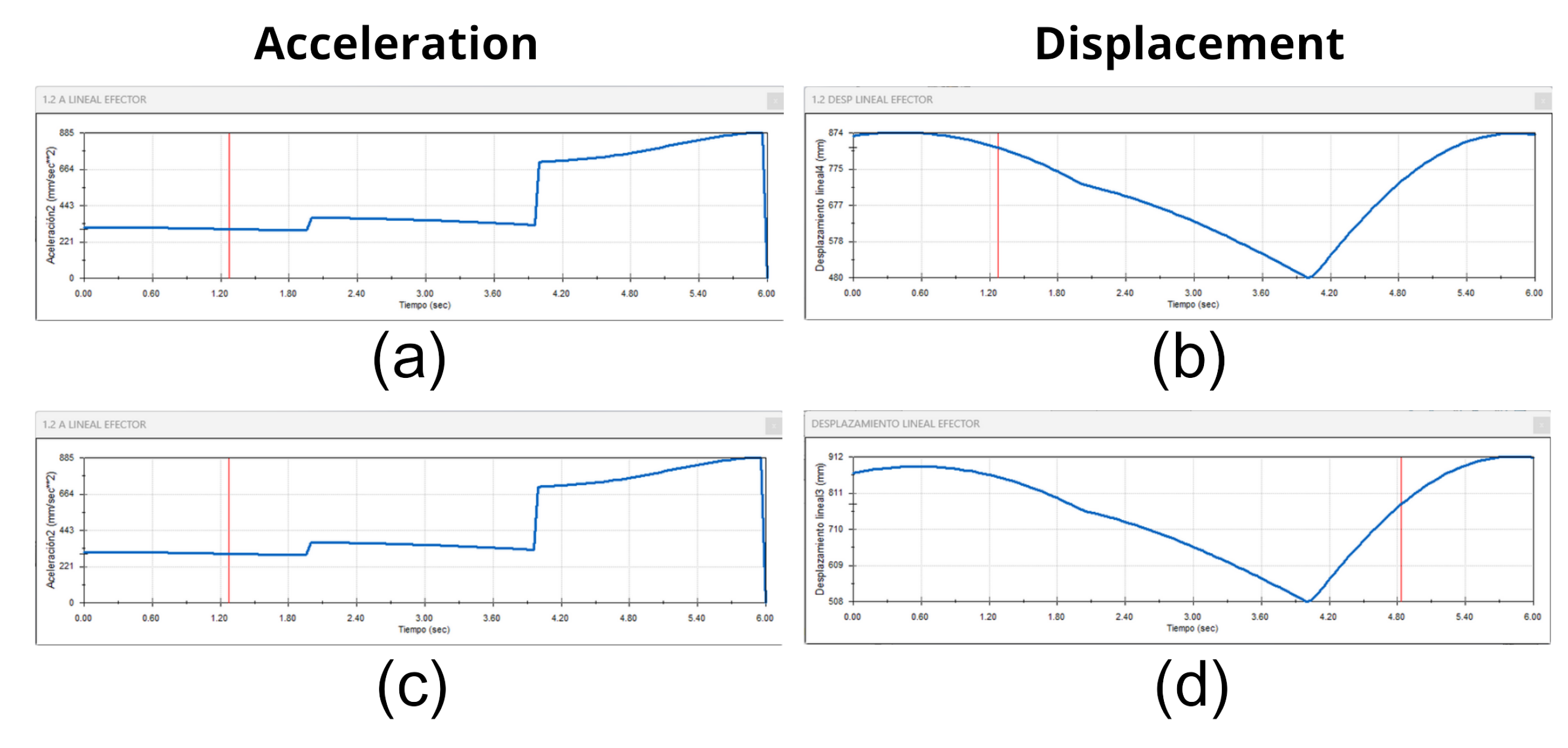
This graph compares the position where the end effector would be attached to the robot with the acceleration with which it moves through the workspace. Mainly, we can observe something very important, which is the position where the end effector would be, which meets the height extension requirement. Without the extension, the effector is at a height of 874mm, and with the extension enabled, it shows an increase to 912mm. The displacement acceleration is equal in both cases of extension; it moves with an acceleration of 885 .
4.4. Systems Integration
A control panel was built with all the necessary elements to effectively control the robot and assign monitoring routines so that the final effector can capture the necessary images for the corresponding analysis.
Figure 26.
Robot controller - Control Panel.

Once all the systems had been developed and tested individually, it proceeded with the integration of all the systems into a single final assembly, which was then tested to verify that all the systems could fit together as expected and interact as a single final product.
In Figure 27, a clear real-time development of the robot during plantation monitoring is evident. This visualization provides detailed insights into the robot’s movements and operational processes within the agricultural setting.
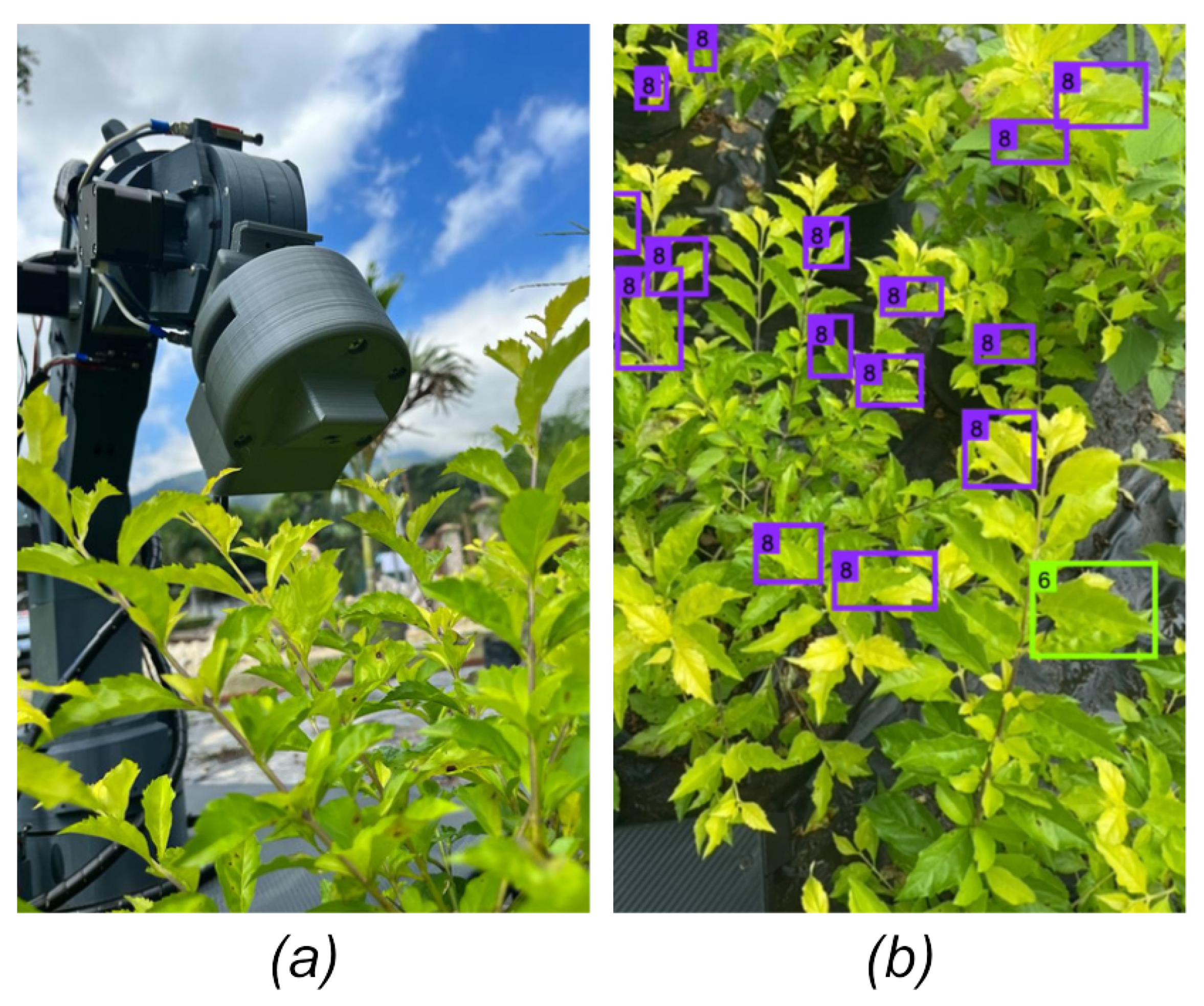
In Figure 28, we showcase the successful integration of the robot with its end effector, which incorporates a specialized camera. This camera is a pivotal component for real-time disease detection in tomato plants. The graphic vividly illustrates how the robot, with its sophisticated end effector, efficiently carries out the crucial function of identifying diseases in real-time, contributing to the overall health management of the tomato crops.
It’s important to underscore the project’s specific focus on a robot tailored for optimizing the health of tomato plants. In Figure 27a, a comprehensive overview of the robot is presented, providing a contextual understanding of its design and capabilities. Zooming in on Figure 27b, we witness the precise moment when the robot detects a specific disease (Yellow Leaf Curl) in the plants, emphasizing the practical application and impact of this technology in enhancing the agricultural landscape. This technological approach, integrating real-time monitoring and disease detection, emerges as a valuable and transformative tool for elevating the health and performance of tomato crops.
5. Related Works
A great deal of effort has been put in by numerous specialists to identify plant diseases because they are a major danger to plant growth and agricultural productivity. In the past, experts have diagnosed plant diseases using visual inspection; biological investigation is a fallback method in case something goes wrong. Recent advances in technology have made it possible to train and detect plant diseases through the widespread use of machine learning.
In [35] focuses on employing a deep learning method based on convolutional neural networks (CNN) for the real-time detection of illnesses in apple leaves. Several CNN models, including VGGNet, ResNet, and Inception-v3, were employed as feature extractors, and Faster R-CNN and SSD were integrated with other object identification models. This study emphasizes the value of precision in the identification of diseases and the application of data augmentation strategies to avoid overfitting.
Using attention modules, the research proposes an enhanced YOLOv5 model for strawberry illness detection. The key improvements are CBAM, involution layer, CARAFE operator, and GhostConv. YOLO-GI, the suggested model, strikes the ideal balance between complexity and performance. Accuracy and recall are enhanced by the addition of the CARAFE operator. This study emphasizes how crucial it is to maximize model complexity in order to enhance plant disease detection efficacy [36].
The use of computer vision technologies for plant disease detection and categorization. It draws attention to the availability of big databases with pictures of both healthy and diseased crop leaves, such as PlantVillage and PlantDoc. The paper emphasizes the necessity of appropriate models for disease identification in field settings and makes the case that accuracy could be increased by combining model assembly and image segmentation [33].
The study [34] uses artificial neural networks with feature selection and CNN models improved with transfer learning to classify early diseases in mango leaves. It draws attention to the necessity for more training photos in real-world settings. The study looks at models like ResNet-50, AlexNet, and VGG16 and emphasizes how crucial feature selection is to enhancing ANN models’ performance. This work shows the necessity for unique datasets for plants of interest, such mango leaves, and offers architectural insights on CNN models.
According to these studies, convolutional neural networks have been successfully used in the field of disease identification on a large scale. Nevertheless, no integrated 7-DOF robot that uses neural networks for disease detection in tomato plants has been designed or developed, despite the possibility of its wide practical applicability in agricultural settings. Therefore, we present such a model in our study.
6. Conclusion
The creation of this robot with its end effector for tomato plant detection highlights the importance of automation in tomato plant health. This technology contributes significantly to the accuracy in identifying diseases allowing for targeted interventions to tomato plants. The design and development of this robot highlights advances in robotics, having the potential to improve efficiency in movement for detection along with the effector. With its 5 degrees of rotational freedom it allows variability in movement with the complexity of movement and together with its prismatic axes allows a greater height that gives us extra movement.
Abbreviations
The following abbreviations are used in this manuscript:
| DOF | Degrees of Freedom |
| FDM | Fused Deposition Modeling |
| CAD | Computer Aided design |
| ABS | Acrylonitrile butadiene styrene |
| FOS | Factor of Safety |
| TPO | Pulse Train Output |
| IOT | Internet Of Things |
| AI | Artifitial Inteligence |
| DL | Deep Learning |
| TL | Transfer Learning |
| mAP | Average Precision |
| PAN | Path Aggregation Network |
| NAS | Neural Architecture Search |
| BiFPN | Bidirectional Feature Pyramid Network |
| ASFF | Adaptive Spatial Feature Fusion |
| SFAM | Selective Feature Aggregation Module |
References
- Sensors | Free Full-Text | Perceptual Soft End-Effectors for Future Unmanned Agriculture.
- Kim, J.; Kim, S.; Ju, C.; Son, H.I. Unmanned Aerial Vehicles in Agriculture: A Review of Perspective of Platform, Control, and Applications. IEEE Access 2019, 7, 105100–105115. [Google Scholar] [CrossRef]
- Chen, Z.; Zeng, Z.; Shu, G.; Chen, Q. Kinematic solution and singularity analysis for 7-DOF redundant manipulators with offsets at the elbow 2018. pp. 422–427. [CrossRef]
- Terreran, M.; Barcellona, L.; Ghidoni, S. A general skeleton-based action and gesture recognition framework for human–robot collaboration. Robotics and Autonomous Systems 2023, 170, 104523. [Google Scholar] [CrossRef]
- Saveriano, M.; Abu-Dakka, F.J.; Kyrki, V. Learning stable robotic skills on Riemannian manifolds. Robotics and Autonomous Systems 2023, 169, 104510. [Google Scholar] [CrossRef]
- Robotics | Free Full-Text | Neural Network Mapping of Industrial Robots’ Task Times for Real-Time Process Optimization.
- Riboli, M.; Jaccard, M.; Silvestri, M.; Aimi, A.; Malara, C. Collision-free and smooth motion planning of dual-arm Cartesian robot based on B-spline representation. Robotics and Autonomous Systems 2023, 170, 104534. [Google Scholar] [CrossRef]
- Gong, M.; Li, X.; Zhang, L. Analytical Inverse Kinematics and Self-Motion Application for 7-DOF Redundant Manipulator. IEEE Access 2019, 7, 18662–18674. [Google Scholar] [CrossRef]
- Zhang, Z.; Yan, Z. An Adaptive Fuzzy Recurrent Neural Network for Solving the Nonrepetitive Motion Problem of Redundant Robot Manipulators. IEEE Transactions on Fuzzy Systems 2020, 28, 684–691. [Google Scholar] [CrossRef]
- Miteva, L.; Yovchev, K.; Chavdarov, I. Planning Orientation Change of the End-effector of State Space Constrained Redundant Robotic Manipulators 2022. pp. 51–56. [CrossRef]
- Ando, N.; Takahashi, K.; Mikami, S. Disposable Soft Robotic Gripper Fablicated from Ribbon Paper with a Few Steps of Origami Folding 2022. pp. 1–4. [CrossRef]
- Samadikhoshkho, Z.; Zareinia, K.; Janabi-Sharifi, F. A Brief Review on Robotic Grippers Classifications 2019. pp. 1–4. ISSN: 2576-7046. [CrossRef]
- Woliński; Wojtyra, M. An inverse kinematics solution with trajectory scaling for redundant manipulators. Mechanism and Machine Theory 2024, 191, 105493. [Google Scholar] [CrossRef]
- Finite-Time Convergence Adaptive Fuzzy Control for Dual-Arm Robot With Unknown Kinematics and Dynamics \textbar IEEE Journals & Magazine \textbar IEEE Xplore.
- Zribi, S.; Knani, J.; Puig, V. Improvement of Redundant Manipulator Mechanism performances using Linear Parameter Varying Model Approach 2020. pp. 1–6. ISSN: 2378-3451. [CrossRef]
- Balaji, A.; Ullah, S.; Das, A.; Kumar, A. Design Methodology for Embedded Approximate Artificial Neural Networks 2019. pp. 489–494. [CrossRef]
- Mangal, R.; Nori, A.V.; Orso, A. Robustness of neural networks: a probabilistic and practical approach 2019. pp. 93–96. [CrossRef]
- Liu, X.; Li, P.; Meng, F.; Zhou, H.; Zhong, H.; Zhou, J.; Mou, L.; Song, S. Simulated annealing for optimization of graphs and sequences. Neurocomputing 2021, 465, 310–324. [Google Scholar] [CrossRef]
- Nakai, T.; Nishimoto, S. Artificial neural network modelling of the neural population code underlying mathematical operations. NeuroImage 2023, 270, 119980. [Google Scholar] [CrossRef]
- Vu, M.N.; Beck, F.; Schwegel, M.; Hartl-Nesic, C.; Nguyen, A.; Kugi, A. Machine learning-based framework for optimally solving the analytical inverse kinematics for redundant manipulators. Mechatronics 2023, 91, 102970. [Google Scholar] [CrossRef]
- Adaptive Projection Neural Network for Kinematic Control of Redundant Manipulators With Unknown Physical Parameters.
- Machines \textbar Free Full-Text \textbar A Collision Avoidance Strategy for Redundant Manipulators in Dynamically Variable Environments: On-Line Perturbations of Off-Line Generated Trajectories.
- Alatise, M.B.; Hancke, G.P. A Review on Challenges of Autonomous Mobile Robot and Sensor Fusion Methods. IEEE Access 2020, 8, 39830–39846. [Google Scholar] [CrossRef]
- Rose, D.C.; Bhattacharya, M. Adoption of autonomous robots in the soft fruit sector: Grower perspectives in the UK. Smart Agricultural Technology 2023, 3, 100118. [Google Scholar] [CrossRef]
- Zhong, Z.; Zhang, J.; Qiu, C.; Huang, S. Design of a Framework for Implementation of Industrial Robot Manipulation Using PLC and ROS 2 2022. pp. 41–45. [CrossRef]
- Wu, B. Study of PLC-based industrial robot control systems. 2022, 1094–1097. [Google Scholar] [CrossRef]
- Liu, Z.; Zhang, L.; Qin, X.; Li, G. An effective self-collision detection algorithm for multi-degree-of-freedom manipulator. Measurement Science and Technology 2022, 34, 015901. [Google Scholar] [CrossRef]
- Ganin, P.; Kobrin, A. Modeling of the Industrial Manipulator Based on PLC Siemens and Step Motors Festo 2020. pp. 1–6. [CrossRef]
- Cao, R.; Ma, X.; Yu, C.; Xu, P. Framework of Industrial Robot System Programming and Management Software 2019. pp. 1256–1261. ISSN: 2158-2297. [CrossRef]
- Rehbein, J.; Wrütz, T.; Biesenbach, R. Model-based industrial robot programming with MATLAB/Simulink 2019. pp. 1–5. [CrossRef]
- Kinematics Analysis for a Heavy-load Redundant Manipulator Arm Based on Gradient Projection Method.
- Chouhan, S.S.; Kaul, A.; Singh, U.P.; Jain, S. Bacterial Foraging Optimization Based Radial Basis Function Neural Network (BRBFNN) for Identification and Classification of Plant Leaf Diseases: An Automatic Approach Towards Plant Pathology. IEEE Access 2018, 6, 8852–8863. [Google Scholar] [CrossRef]
- Moupojou, E.; Tagne, A.; Retraint, F.; Tadonkemwa, A.; Wilfried, D.; Tapamo, H.; Nkenlifack, M. FieldPlant: A Dataset of Field Plant Images for Plant Disease Detection and Classification With Deep Learning. IEEE Access 2023, 11, 35398–35410. [Google Scholar] [CrossRef]
- Pham, T.N.; Tran, L.V.; Dao, S.V.T. Early Disease Classification of Mango Leaves Using Feed-Forward Neural Network and Hybrid Metaheuristic Feature Selection. IEEE Access 2020, 8, 189960–189973. [Google Scholar] [CrossRef]
- Jiang, P.; Chen, Y.; Liu, B.; He, D.; Liang, C. Real-Time Detection of Apple Leaf Diseases Using Deep Learning Approach Based on Improved Convolutional Neural Networks. IEEE Access 2019, 7, 59069–59080. [Google Scholar] [CrossRef]
- Chen, S.; Liao, Y.; Lin, F.; Huang, B. An Improved Lightweight YOLOv5 Algorithm for Detecting Strawberry Diseases. IEEE Access 2023, 11, 54080–54092. [Google Scholar] [CrossRef]
- Bochkovskiy, A.; Wang, C.Y.; Liao, H.Y.M. YOLOv4: Optimal Speed and Accuracy of Object Detection 2020. arXiv 2020, arXiv:arXiv:2004.10934. [Google Scholar]
- Asha Rani, K.P.; Gowrishankar, S. Pathogen-Based Classification of Plant Diseases: A Deep Transfer Learning Approach for Intelligent Support Systems. IEEE Access 2023, 11, 64476–64493. [Google Scholar] [CrossRef]
- Kumar, S.; P, P.; Dutta, A.; Behera, L. Visual motor control of a 7DOF redundant manipulator using redundancy preserving learning network. Robotica Cambridge University Press. 2010. [Google Scholar] [CrossRef]
Figure 2.
Process for the Detection of Diseases in Tomato Plants
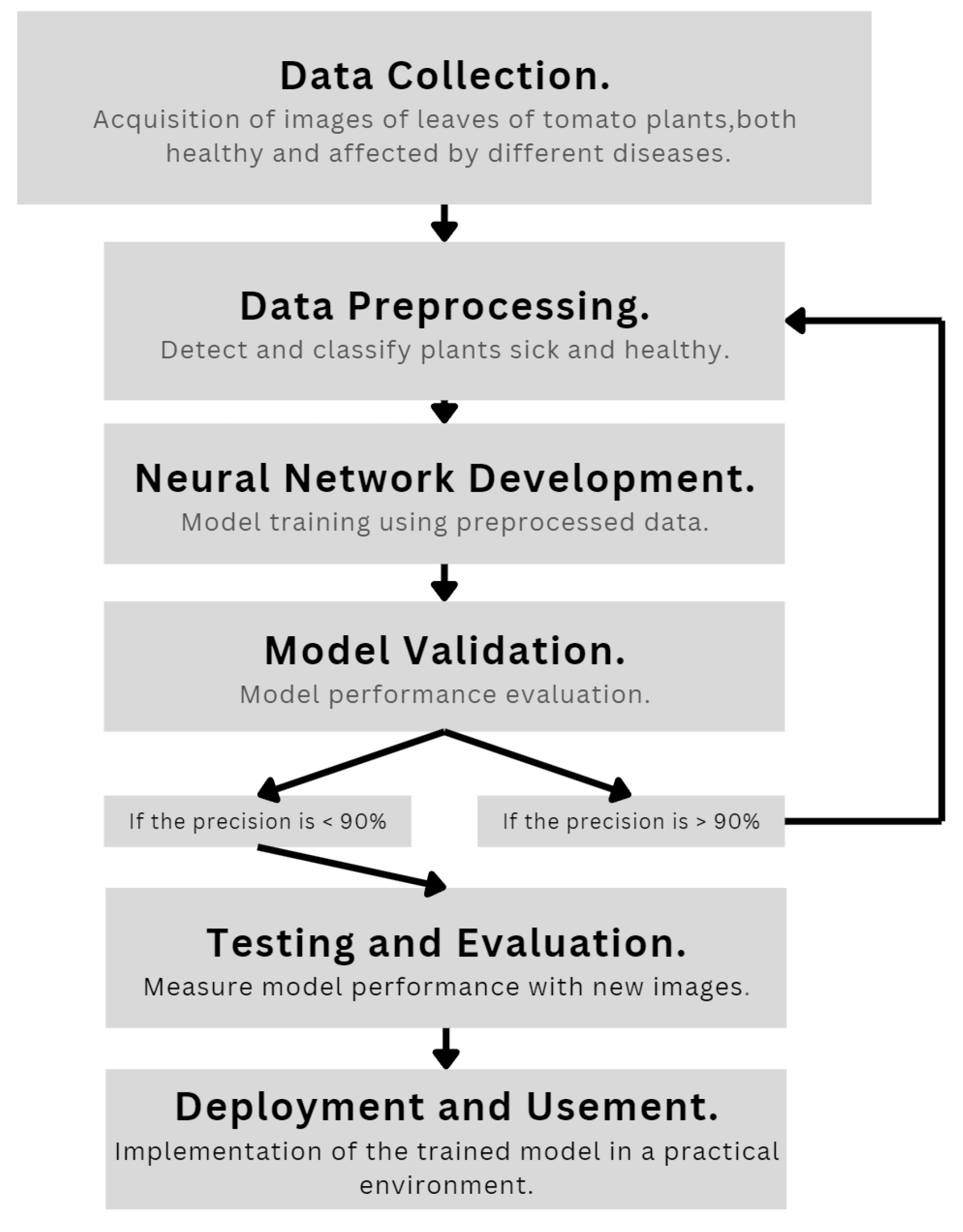
Figure 3.
Tomato Plant Diseases. (a) Early Blight, (b) Healthy Plant, (c) Late Blight, and (d) Leaf Miner.
Figure 3.
Tomato Plant Diseases. (a) Early Blight, (b) Healthy Plant, (c) Late Blight, and (d) Leaf Miner.
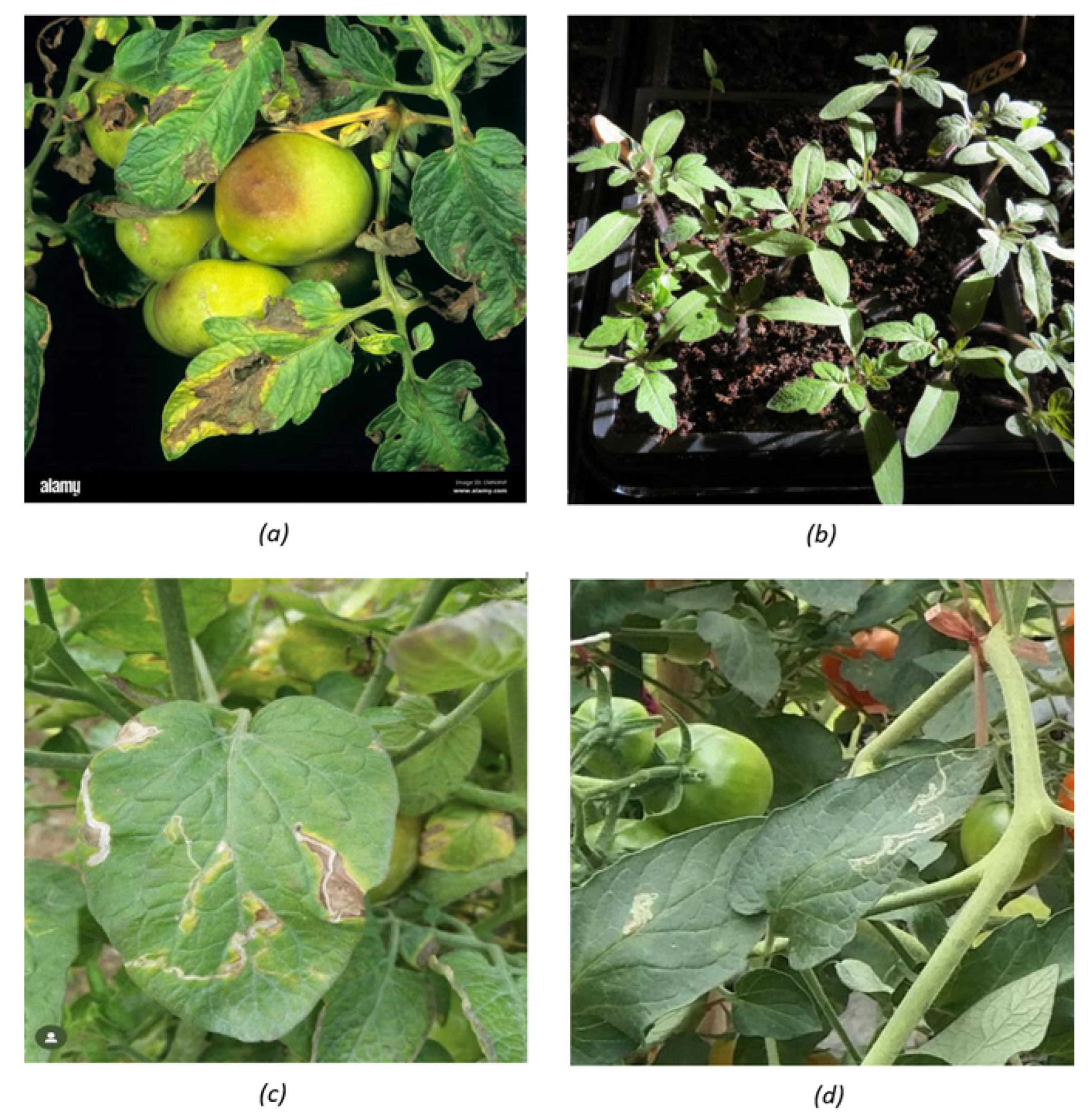
Figure 4.
Annotation of Disease on Tomato Plant Leaves.
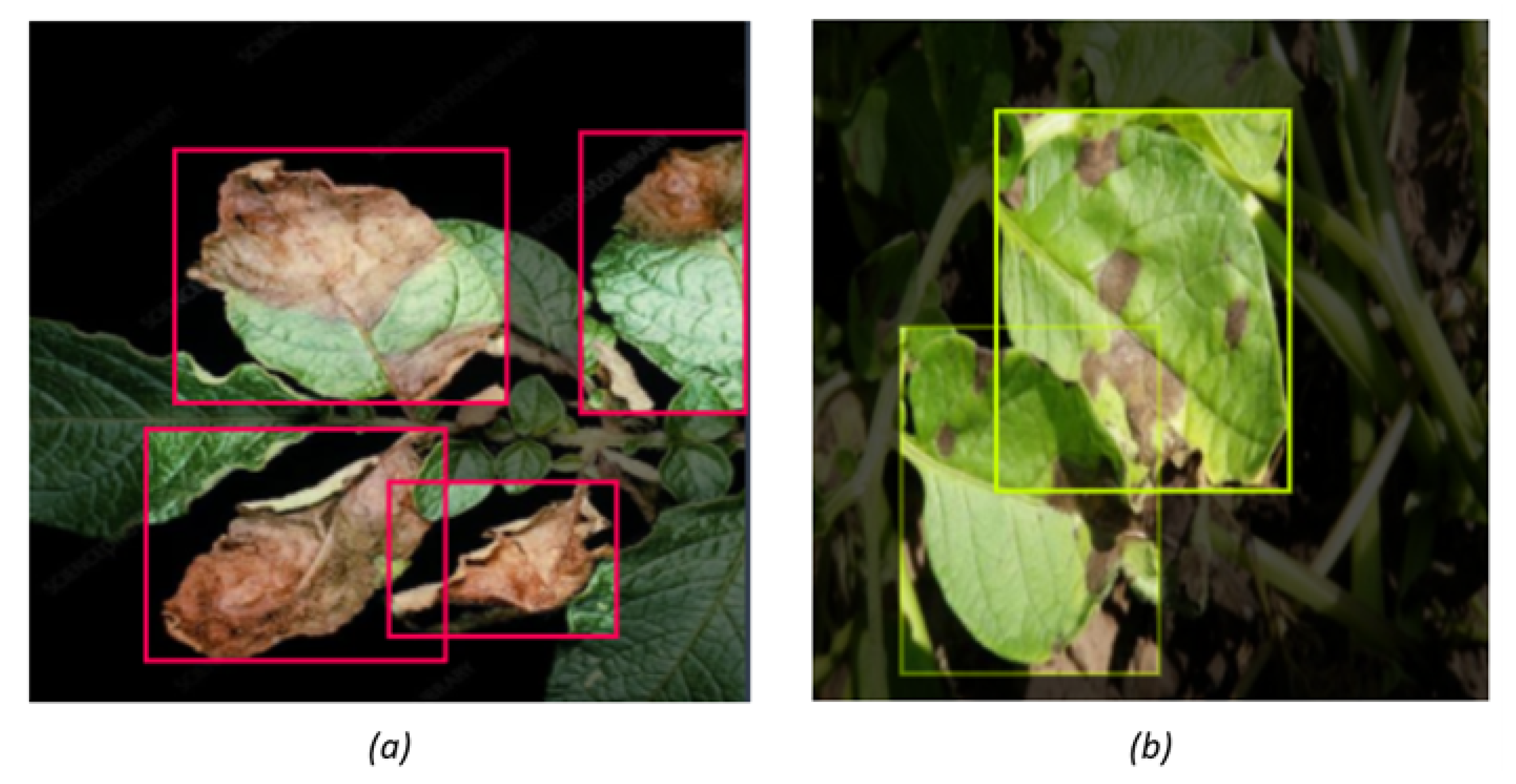
Figure 5.
Confusion Matrix [37]
Figure 5.
Confusion Matrix [37]
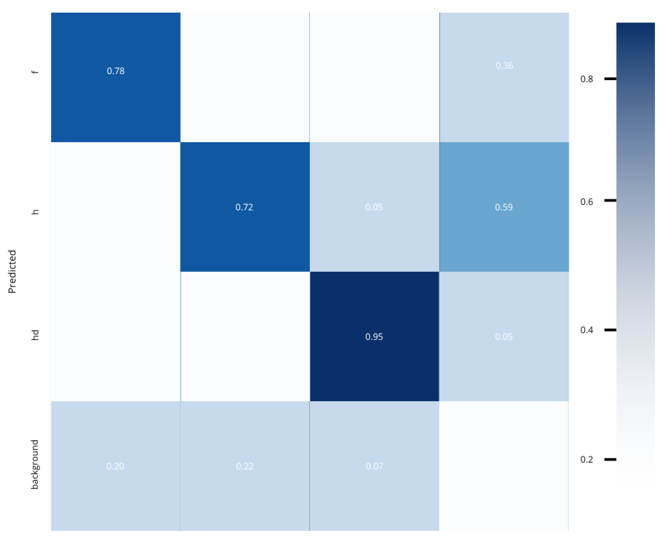
Figure 6.
Object Detection Process [37]
Figure 6.
Object Detection Process [37]
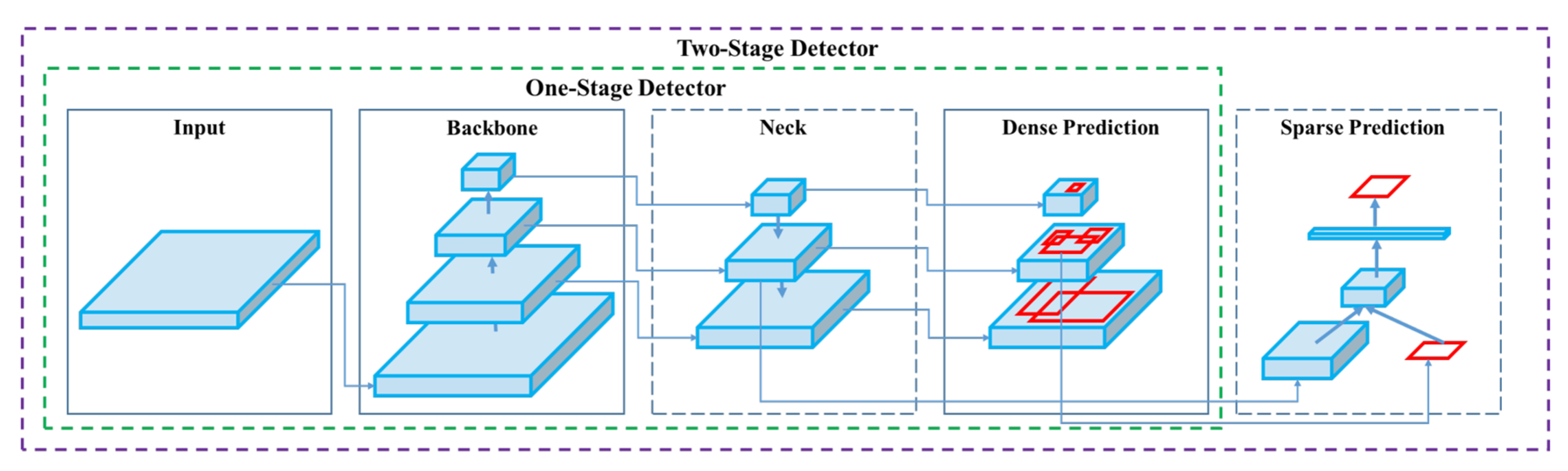
Figure 15.
GExperiment´s mAP Graphs.
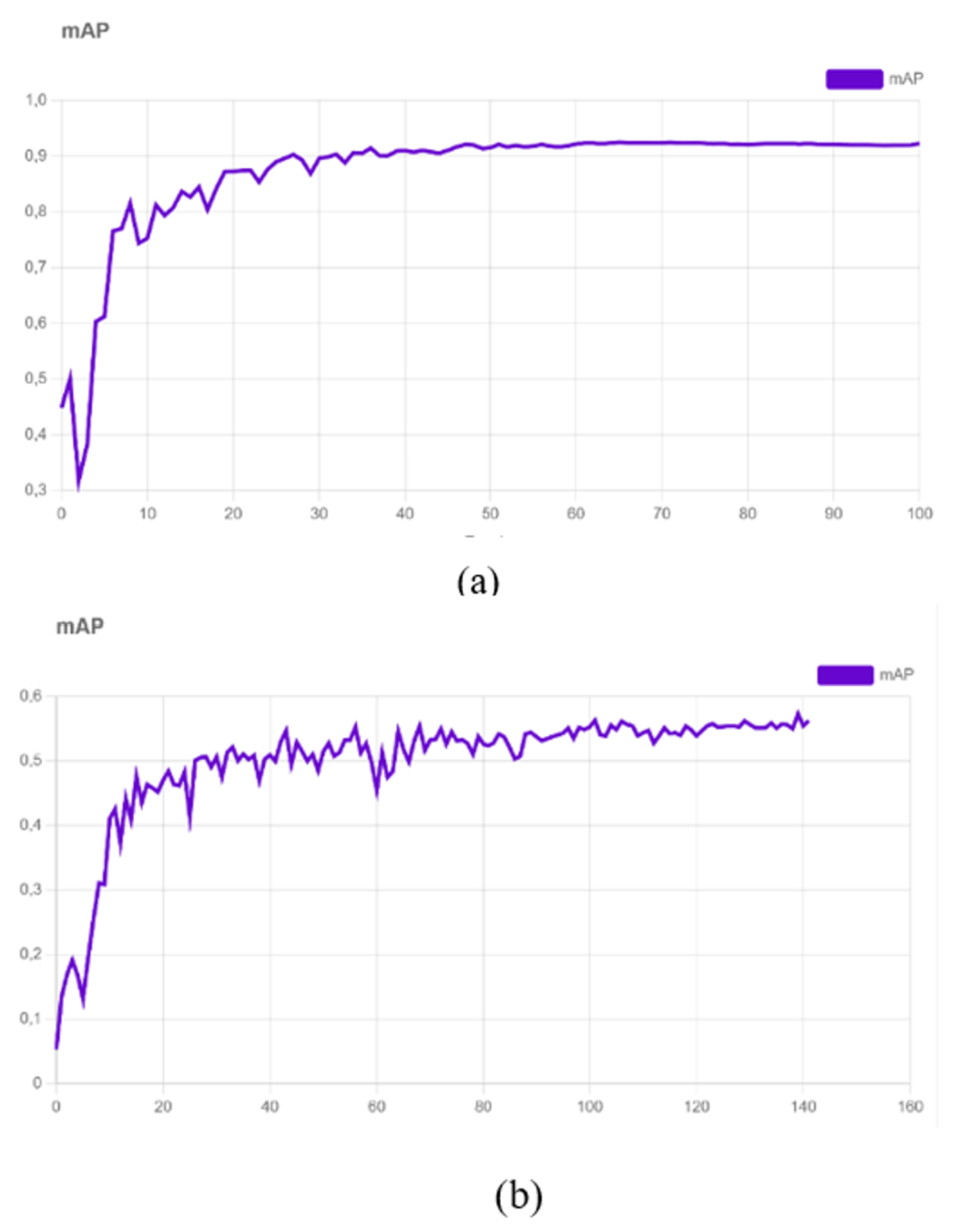
Figure 16.
Experiment´s mAP and Precision.
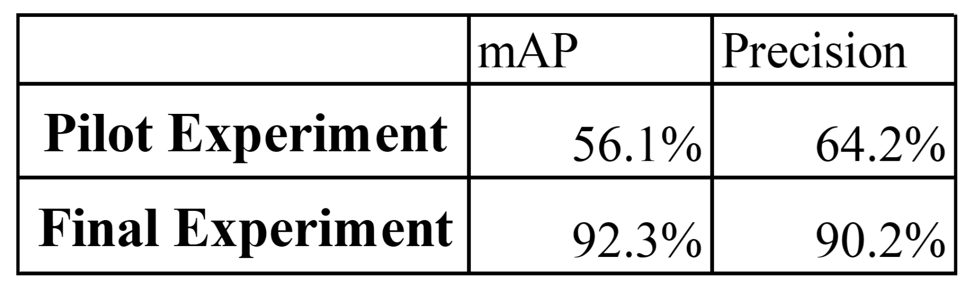
Figure 17.
Disease Accuracy.
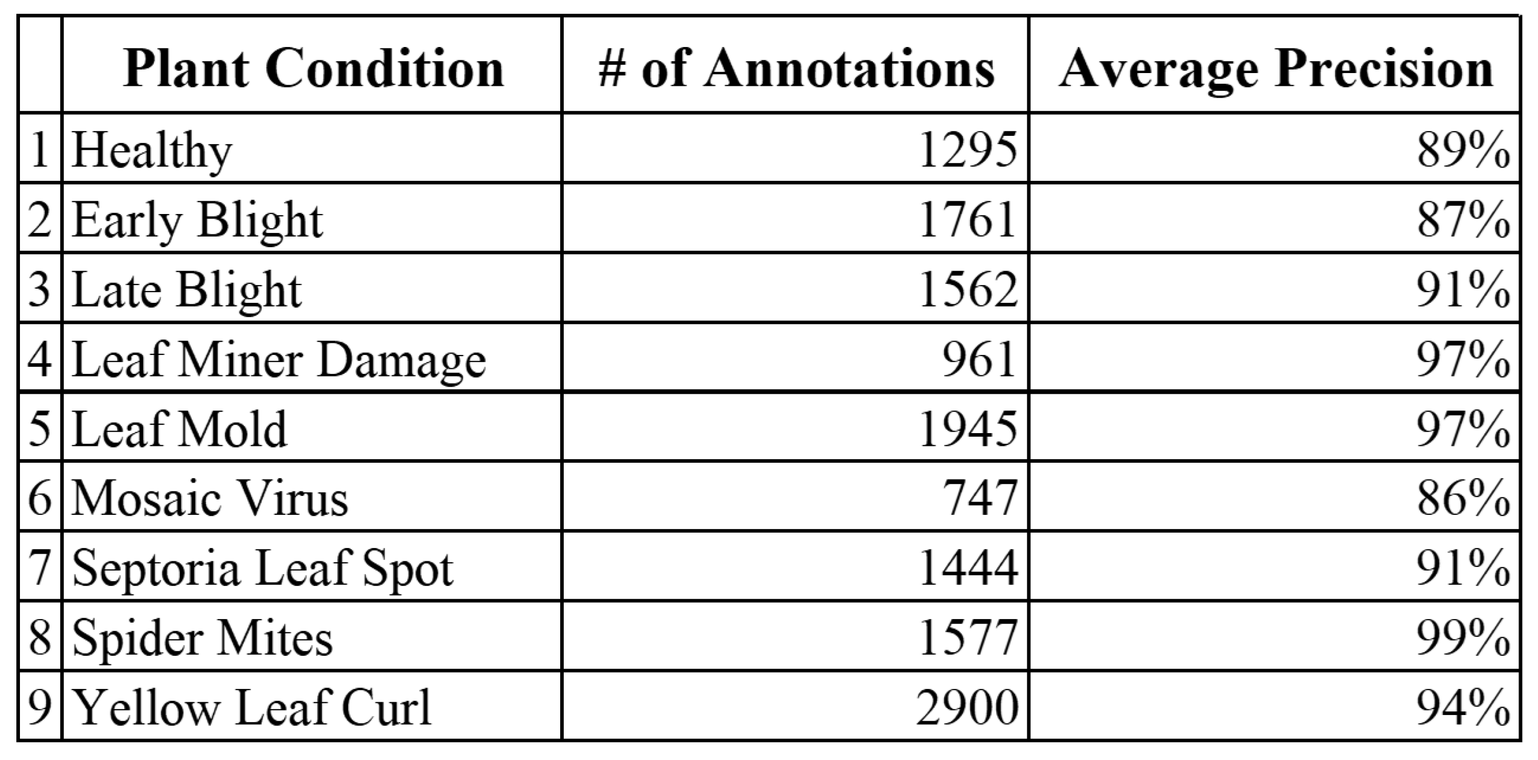
Figure 18.
Diseases: (a) Early Blight, (b) Late Blight, (c) Leaf Miner, (d) Leaf Mold, (e) Mosaic, (f) Septoria Spot, (g) Spider Mites and, (h) Yellow Curl.
Figure 18.
Diseases: (a) Early Blight, (b) Late Blight, (c) Leaf Miner, (d) Leaf Mold, (e) Mosaic, (f) Septoria Spot, (g) Spider Mites and, (h) Yellow Curl.
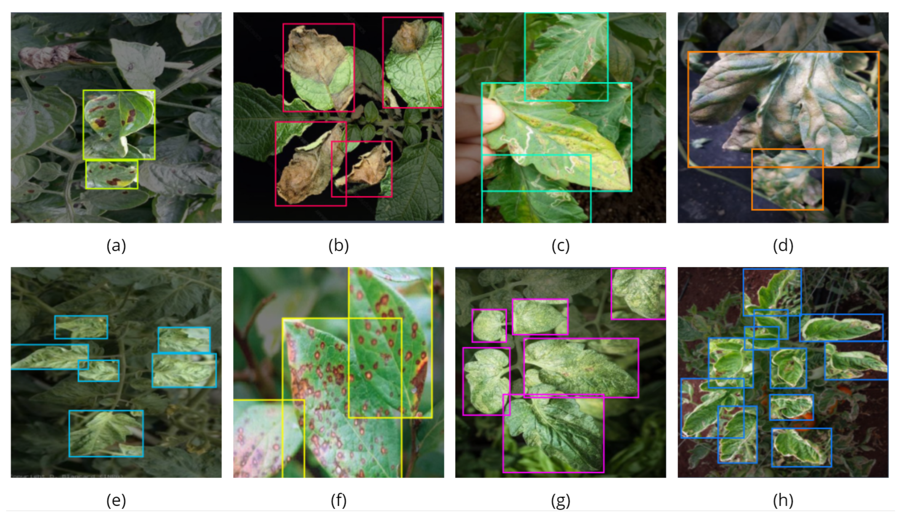
Figure 19.
Real-Time Detection.
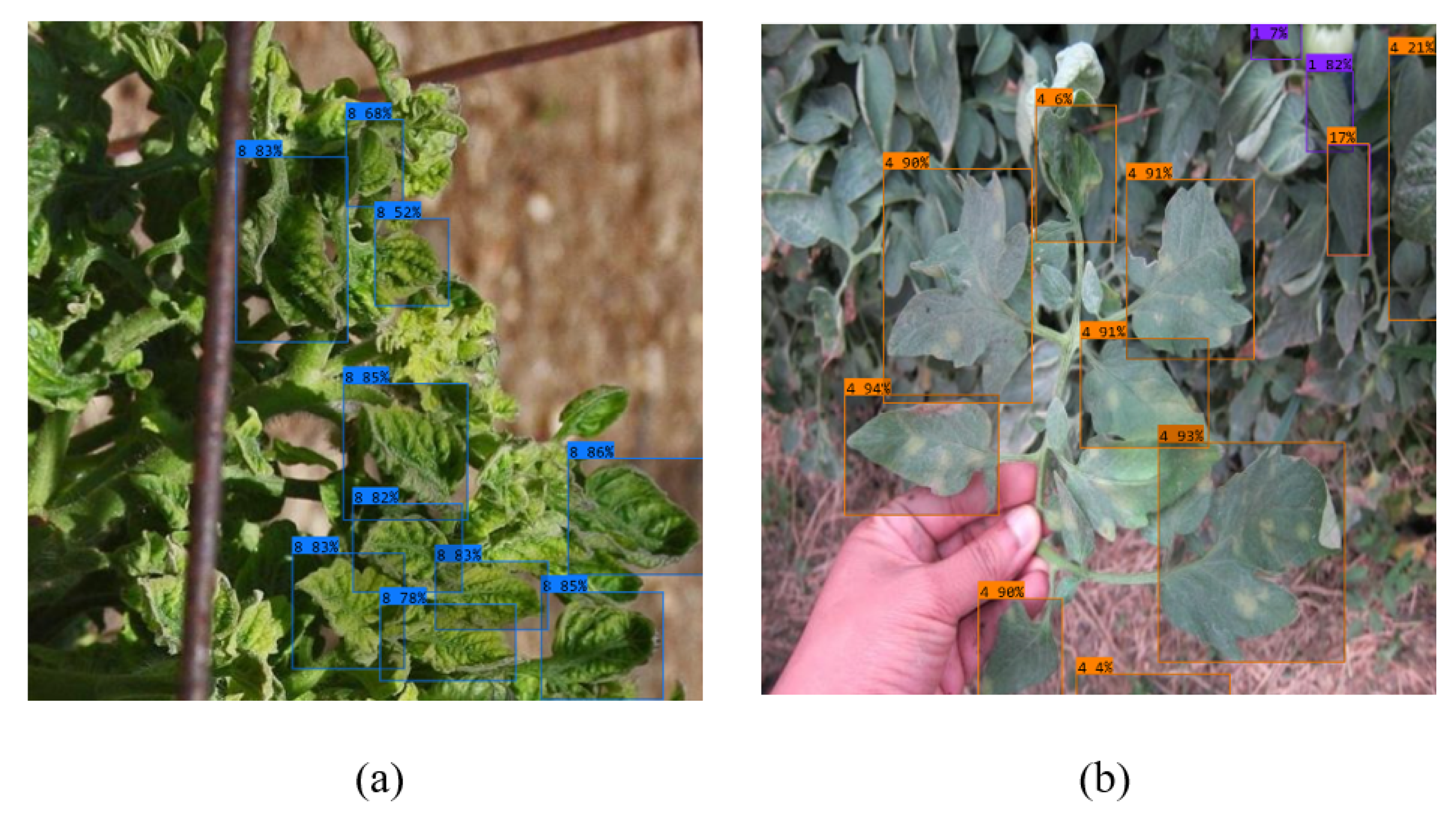
Figure 20.
Final-Effector Design.
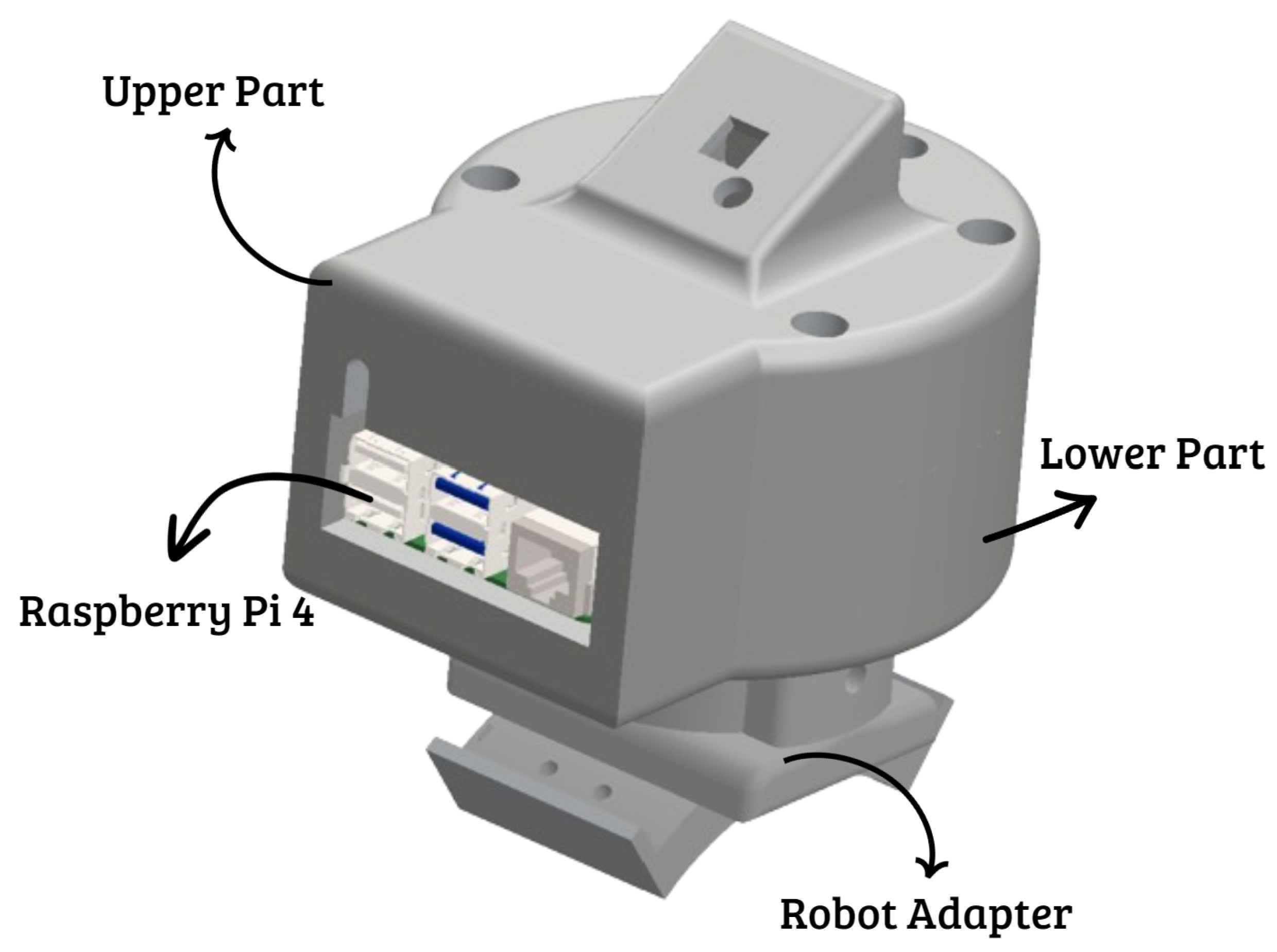
Figure 21.
Rotational actuators- Motor power consumption comparison graphs. Motor 1 shown on graphs a and b. Motor 2 shown on graphs c and d. Motor 3 shown on graphs e and f. Motor 4 shown on graphs g and h. Motor 5 shown on graphs i and j.
Figure 21.
Rotational actuators- Motor power consumption comparison graphs. Motor 1 shown on graphs a and b. Motor 2 shown on graphs c and d. Motor 3 shown on graphs e and f. Motor 4 shown on graphs g and h. Motor 5 shown on graphs i and j.
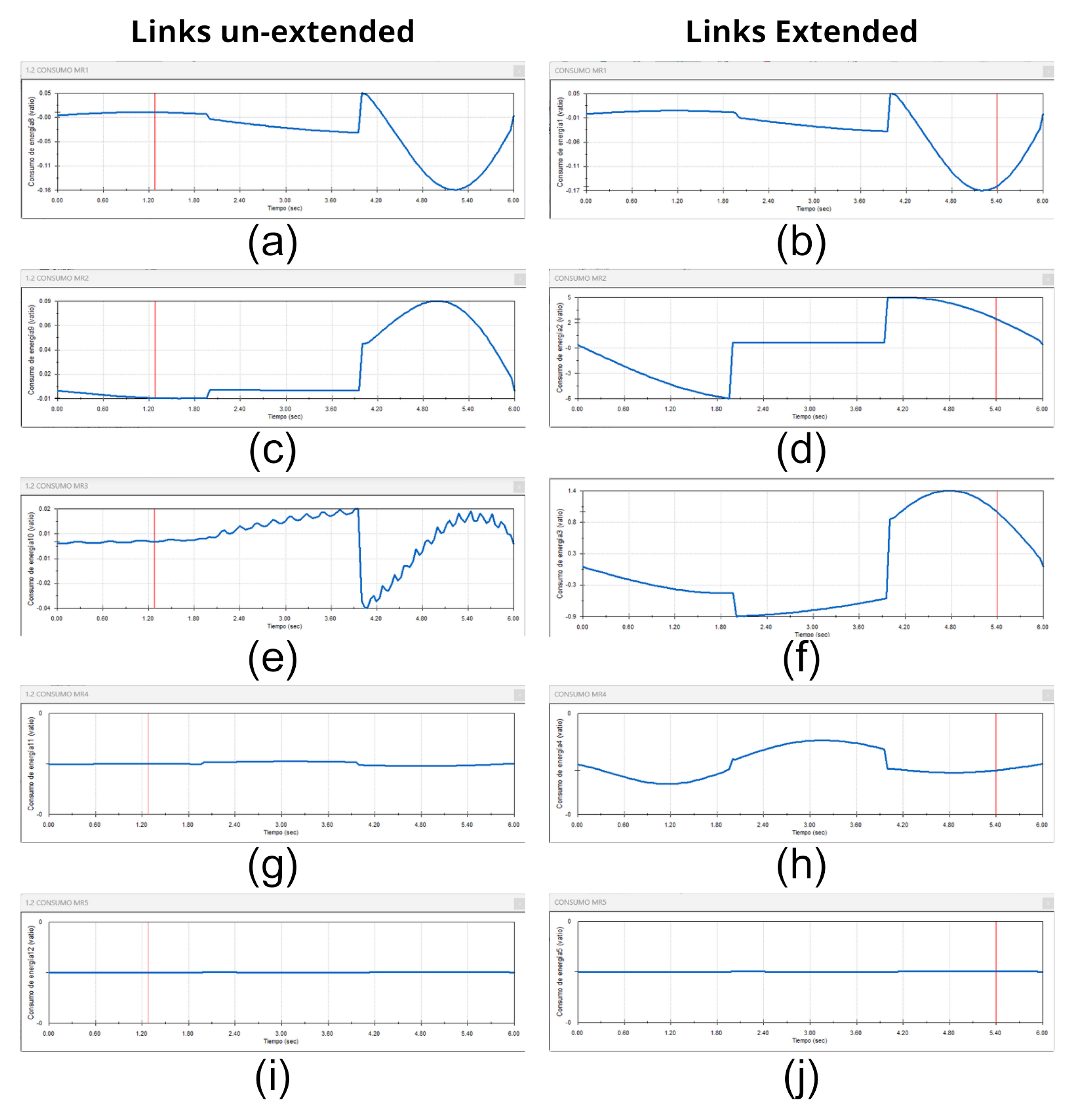
Figure 22.
Rotational actuators- motor torque comparison graphs. Motor 1 shown on graphs a and b. Motor 2 shown on graphs c and d. Motor 3 shown on graphs e and f. Motor 4 shown on graphs g and h. Motor 5 shown on graphs i and j.
Figure 22.
Rotational actuators- motor torque comparison graphs. Motor 1 shown on graphs a and b. Motor 2 shown on graphs c and d. Motor 3 shown on graphs e and f. Motor 4 shown on graphs g and h. Motor 5 shown on graphs i and j.
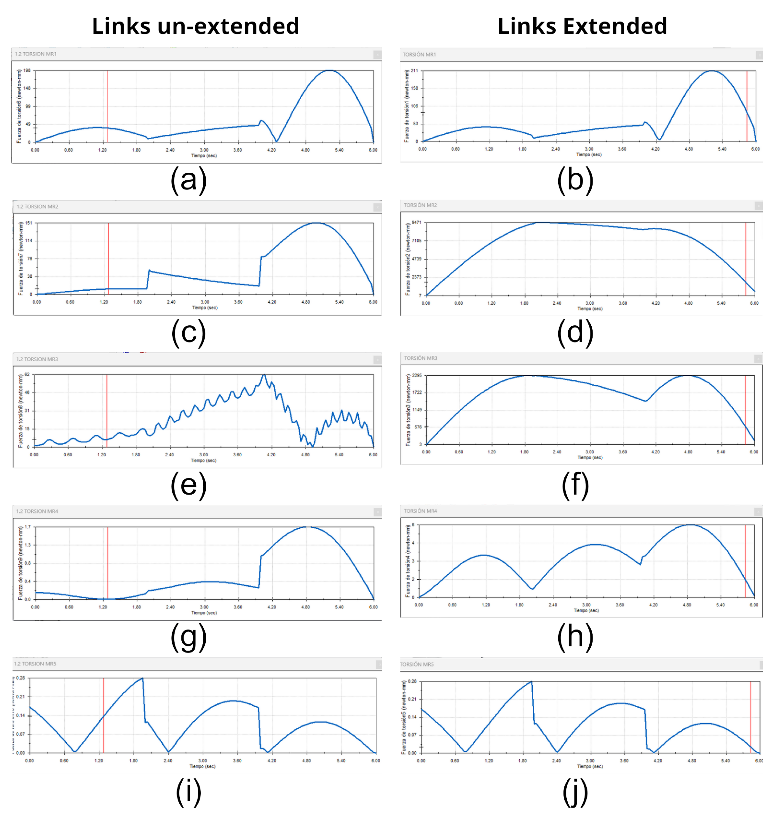
Figure 27.
Final system integration - plant monitoring general view.
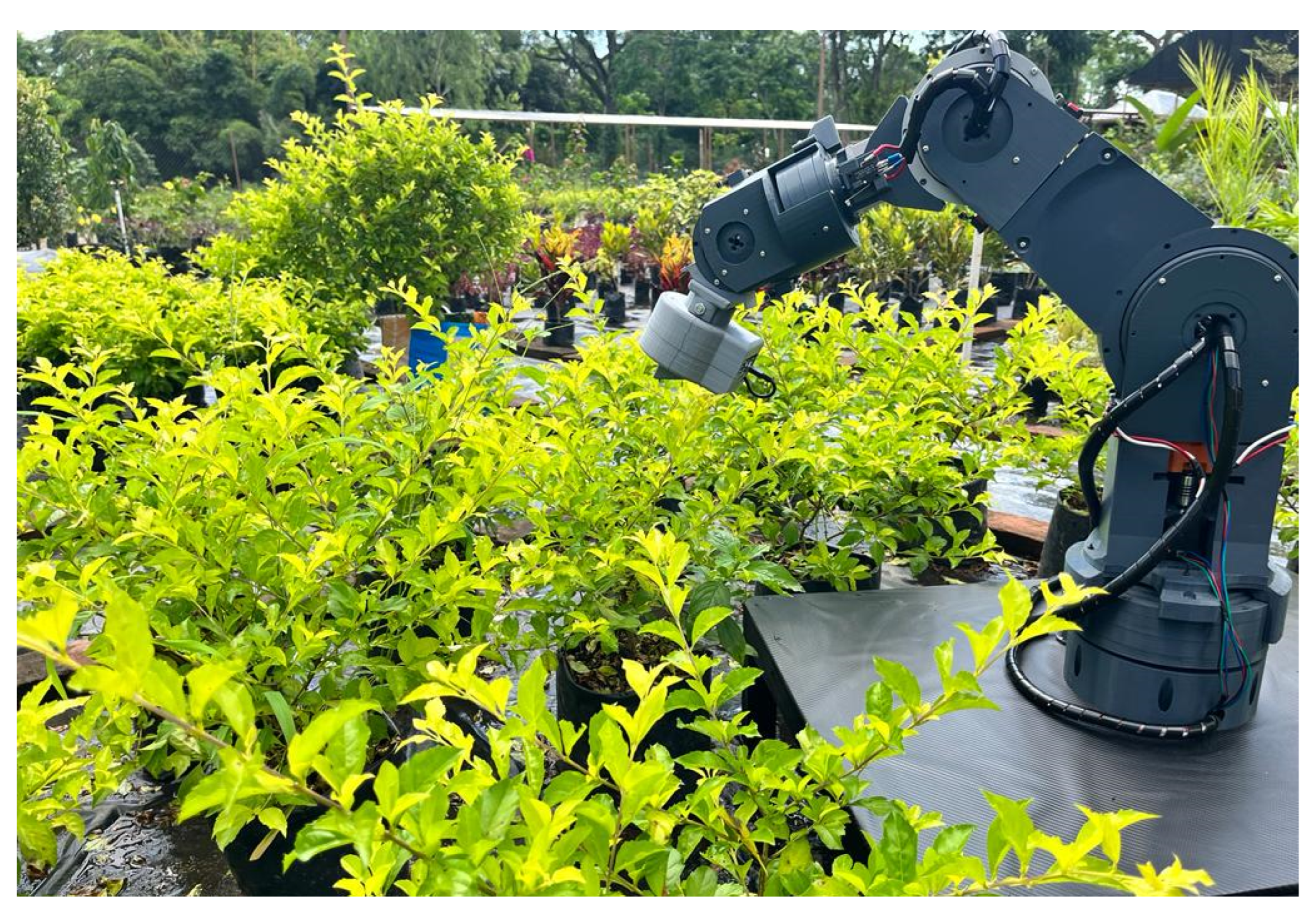
Figure 28.
Final systems integration - (a) The end effector is coupled to the robot in data collection position number one. (b) Neural network that collects data in real time.
Figure 28.
Final systems integration - (a) The end effector is coupled to the robot in data collection position number one. (b) Neural network that collects data in real time.
Disclaimer/Publisher’s Note: The statements, opinions and data contained in all publications are solely those of the individual author(s) and contributor(s) and not of MDPI and/or the editor(s). MDPI and/or the editor(s) disclaim responsibility for any injury to people or property resulting from any ideas, methods, instructions or products referred to in the content. |
© 2025 by the authors. Licensee MDPI, Basel, Switzerland. This article is an open access article distributed under the terms and conditions of the Creative Commons Attribution (CC BY) license (http://creativecommons.org/licenses/by/4.0/).
Copyright: This open access article is published under a Creative Commons CC BY 4.0 license, which permit the free download, distribution, and reuse, provided that the author and preprint are cited in any reuse.


