
Submitted:
11 October 2025
Posted:
13 October 2025
You are already at the latest version
Abstract
In this paper, we show that the reported excess in the matter cosmological dipole relative to the cosmic microwave background dipole is primarily a result of errors in the procedures used to extract the dipole from observations of radio galaxies and quasars. The basis of all the work done to date is a formula given by Ellis and Baldwin (EB) in their 1984 paper. The main issue is that this formula is only valid when applied to a collection of galaxies isotropic in the source rest frame whereas, in practice, it is being applied to collections obtained using a uniform flux cutoff in the observer frame. The result is a collection that is not isotropic in the source frame and so violates the conditions required for the validity of the EB result. We rst provide a qualitative description of the source of this excess and then develop a new formula that can be applied to the observer frame data set. Analysis with this new formula eliminates about 80% of the reported dipole discrepancy in the quasar case. In the radio galaxy case, the corrected analysis of the published results removes only about 30% of the discrepancy but we then go on to show that the remaining large discrepancy between the radio galaxy and CMB dipoles is a consequence of a flux cutoff that is set too low. After an upward adjustment of the cutoff , the predicted dipole in the radio galaxy case is the same as the quasar dipole prediction.
Keywords:
cosmic dipole
; quasar dipole
; galaxy dipole
; standard model tension
1. Introduction
During the past two decades, there has been considerable interest in what we will term the dipole problem, [1]. In a homogeneous and isotropic universe, it is generally agreed that in the cosmic rest frame, the portion of the cosmic microwave background (CMB) radiation above some minimal intensity cutoff should be homogeneous and isotropic on large scales. That being the case, the observed dipole moment of the CMB radiation must be a consequence of the peculiar velocity of our galaxy with respect to the cosmic rest frame. Cosmological models in general also suppose that, aside from their peculiar velocities, structures such as galaxies are at rest in the cosmic rest frame so they should exhibit the same dipole as the CMB. The problem is that recent studies, [2,3,4,5] and references therein, seem to show a significant departure from this expectation, namely that the material dipoles so determined have amplitudes at least twice that of the CMB. The conclusion that followed is that the cosmological models must be wrong and that there must exist very large inhomogeneous cosmological structures in violation of the cosmological principle with amplitudes large enough to explain the measured dipole. We agree that the standard model is wrong and that there do exist such structures and that they likely contribute to the apparent disparity but we don’t agree that such homogeneities lead to a matter dipole that is something other than the peculiar velocity dipole.
There are reasons to be skeptical of the reported excess. We know from observations of nearby galaxies that the Milky Way does have a peculiar velocity and that the measured CMB dipole really is a dipole which supports the idea that the dipole is a consequence of that peculiar motion. There is a quadrupole contribution to the CMB anisotropy but its magnitude is about 2 orders of magnitude smaller than that of the dipole. This means that no matter what else is going, in the matter case, the peculiar velocity dipole must be part of the mix. The next fact is that the measured matter dipole is in fairly close alignment with the CMB dipole which means that if a significant portion of the dipole is not a result of our peculiar velocity, the unknown source would have needed to somehow align itself with our peculiar velocity long before our present-day peculiar velocity even existed and that is clearly an impossibility.
It is much easier to believe that there is something seriously wrong with the dipole analysis. The measurement of the CMB dipole is conceptually simple. One measures the temperature of the CMB across the whole sky and then extracts the dipole portion of the anisotropy. This is simple because there is only one CMB and we determine the dipole directly from the radiation. Extracting the dipole from a distribution of material objects, however, is a different matter altogether because the apparent dipole distribution of the objects, of which there is a huge number, is only indirectly related to the radiation we receive from those objects.
The beginnings of this effort date back to the 1984 paper by Ellis and Baldwin, [6], hereafter EB. In that paper, the authors argue that the detection of the dipole can be reduced to just a matter of counting galaxies. But, counting galaxies by itself tells us nothing about the dipole if we don’t know what count to expect. The peculiar motion of our galaxy also causes a shift in the observed frequencies of the radiation coming from those galaxies but that again tells us nothing useful unless we also know something about what spectrum to expect.
The crux of the matter is that the formula from EB upon which all the dipole studies are based is only valid for collections of galaxies isotropic in the source rest frame and for this to be true, the source flux lower cutoff must also be isotropic in the source frame. In practice, however, the collections of galaxies are selected based on a uniform flux cutoff in the observer rest frame and consequently are not isotropic in the source frame. The result is an apparent exaggeration of the dipole relative to the CMB dipole. To resolve this issue, one must either select galaxies based on a source frame cutoff or derive a new formula that allows the observer frame data set to be used. Since it is not possible in practice to apply a uniform flux cutoff in the source frame, we are left with the 2nd option. In this paper, we have derived a replacement for the EB formula that is valid for the observer frame data set, and with its use, most of the dipole problem disappears.
To understand the dipole problem and its solution, it is necessary to have a clear understanding of both the formulas quoted in EB and the accompanying constraints. Unfortunately, that paper does not contain any development nor is there sufficient emphasis placed on the critical constraints embedded in their final result. These shortcomings make it easy to go astray when applying their formula so we will begin by working our way through the development to the EB final result.
2. Background
We deal with two reference frames. The first is the rest frame of the sources which we will indicate with a prime and the other is the rest frame of the observer with quantities written without a prime, i.e. versus X. Also, we will use the letter f instead of the commonly used to denote frequency to avoid confusion with the similar letter v that we use to denote velocity.
We begin with the relativistic Doppler effect. The relativistic equations presented here follow the discussion in [7,8]. For an observer traveling with a velocity of magnitude at an angle relative to a source of radiation, the observed frequency of the radiation will be doppler-shifted by an amount where
The convention used in both EB and [8]. is that when the observer is approaching the source. We mention this only because it is more common in discussions of special relativity to use the opposite convention. The angle that appears in this equation is defined in the source rest frame.
The connection between the angle seen by the observer, , and is given by the formula for relativistic aberration,
Using this formula, Equation (1) can be transformed into
An element of solid angle in the source frame is given by . In the observer’s frame, we have which we need to relate to the source frame formula. The azimuthal angle is not affected by the boost so . Inverting Equation (2) gives
Up to this point, the transformations between frames are probably familiar even if the details are hazy. We now need to relate the flux seen in one frame to that seen in the other. The radiation energy passing through an area in a time is related to the specific intensity of the radiation by where is the angular size of the source as seen by the observer, [7]. The term "specific" indicates that the quantity is per frequency interval, i.e. . Because the sources (galaxies) are far away the angle is very small so . The result is
This has the units of . We now make use of the fact that the quantity is a Lorentz invariant, [8]. Thus,
The final steps make use of two empirical relationships. The first states that the spectra of actual cosmological sources can be reasonably approximated by the formula
Inserting into Equation (9), we have
The quantity (denoted in EB) is the flux that the observer would detect if at rest in the source rest frame. This equation gives the observed specific flux as a function of the observation angle coming from a distribution of sources in which, by assumption, the observed frequency is chosen to be the same as the radiated frequency. The observed flux does vary with frequency but that frequency dependence is contained in the factor which is independent of the observation angle. This means that the total flux, which we obtain by integrating over the observed frequency, has the same angular dependence as the specific flux, i.e. .
The second empirical result states that the total count of sources with fluxes greater than some specified cutoff per solid angle is given by
in the rest frame of the sources. We now write
which is the count per solid angle that the observer would experience if at rest in the source rest frame. As we just noted, the integrated flux has the same angular dependence as the specific flux so in Equation (13) whether we refer to the specific or total flux is of no consequence. Combining Equations (11) and (12) gives
Next, we transform into the observer’s rest frame. Numbers are invariant under Lorentz transforms so we only need to apply Equation (7) with the result that
We now use the fact that our peculiar velocity is about so , , , so
We finally have
which is the EB formula. There are two contributions to the dipole amplitude; the first term (=2) is a consequence of the aberration via Equation (7) and the other term, , follows directly from the Doppler frequency shift via Equations (10 – 16) independent of the aberration.
There are three points to be made about this equation. First, the validity of this formula requires a uniform cutoff in the source frame rather than in the observer frame which is nothing more than the requirement that one must base one’s observations on a collection of standard candles in some reference frame if one wants to establish some particular of the observer relative to that frame. In the EB case, the standard candle is the collection of galaxies above some uniform flux cutoff in the source rest frame and if the formula is to be used, all those galaxies above the cutoff and none of the ones below the cutoff must be counted. Applying the formula to any count that omits any of the first set or includes any of the second will yield a set of parameters but they will not be the parameters of the cosmic dipole.
The second point follows from the statement by the authors of EB that while there is considerable leeway in how one applies this test, one must do the same thing in both the forward and backward directions. ”The same thing” means in the source rest frame, not in the observer’s rest frame and it also means that one must be careful not to introduce a bias in the measurements by, for example, using inappropriate masks in the object selection process.
The third point concerns the range of validity of Equation (17). Looking back over the derivation, one sees that, while the flux level is a parameter of the model, its particular value does not enter into the analysis. The analytic forms of Equations (10) and (12) are necessary but the resulting formula, Equation (17) is valid for any flux cutoff as long as the value is within a range for which Equation (12) is a power-law with a constant value of x. We also see that the formula is valid for each value of separately. The consequence is that we can replace the constant with some dependent value and the formula will give the corresponding count in the observer frame for that value of . Replacing it with another value for a different will give the count for that value. One must not forget, however, that the EB formula will not represent the cosmic dipole unless the source distribution is uniform in the source rest frame, i.e. that is a constant.
3. Standard Candles and Consequences
In the previous section, we pointed out the significant constraint that researchers have either failed to appreciate or have chosen to ignore. When researchers have viewed Equation (17), they have seen only the dipole factor and have ignored the constraint that the validity of that equation requires that the flux cutoff must be uniform in the source frame, not the observer’s frame. If one tries to apply the cutoff in the source frame, however, one immediately realizes that it can’t be done. That impossibility, however, does not give researchers a free pass to ignore the requirement. What can, and is, done is to set a uniform flux cutoff in the observer frame but in that case, the EB equation cannot be used to determine the dipole parameters.
Consider the following thought experiment. Imagine that we hop off our galaxy into the source rest frame. While there, we identify a collection of galaxies that includes all galaxies across the sky with fluxes equal to or greater than some uniform flux cutoff. To keep track of our collection, we color the selected galaxies green and the remainder, which have fluxes below the cutoff, blue. The result is shown in Figure 1 which shows the flux (not the counts) versus the observation angle, .
In a homogeneous universe, the count of green galaxies per solid angle will be the same in all directions. However, if for some reason, we fail to count some of the green galaxies in some direction or include blue galaxies in another direction, the counts won’t be uniform.
We now boost back to our galaxy with the result shown in Figure 2.
We find that because of the Doppler shift, Equation (11), the source flux cutoff line is tilted with the fluxes lower in the backward direction and higher in the forward direction. The EB formula tells us that the count of galaxies is also lower in the backward direction and higher in the forward direction but that is not what is shown in the figure.
We now get to the fundamental point. If we are going to use the EB formula to determine the dipole parameters, we must count all the green galaxies and none of the blue galaxies. In Figure 3, we show what observers are actually doing which is to set a uniform flux cutoff in the observer frame.
With this cutoff, we see that instead of counting all the green galaxies down to the sloping line, in the backward direction, those in the purple triangle are omitted from the count because their fluxes are below the observer frame cutoff. Conversely, in the forward direction, the blue galaxies in the orange triangle are included when they should not be because their flux levels are above the observer frame cutoff.
According to EB, the count of green galaxies will be lower than average in the backward direction and because the purple triangle galaxies have been omitted, the actual count will be lower still. In the forward direction, the opposite is true. Counting all the green galaxies will, by themselves, result in a value greater than the average, and adding in the blue galaxies with fluxes in the orange triangle will boost the count even more.
The result is an exaggeration of the apparent dipole.
We now jump back to the source rest frame with the result shown in Figure 4.
We find that uniform observer frame cutoff is sloped in the reverse direction, i.e. greater in the backward direction. Choosing the set of galaxies in the source frame that would match the sloping line is, in reality, impossible to achieve because we, now back in the source rest frame, would have to know which galaxies the observer happens to choose ahead of time.
Thus, while the EB formula is correct, it is not possible to make direct use of it. Since we are stuck with the uniform observer frame flux cutoff, the only option is to develop a replacement for the EB formula.
4. How Much Exaggeration?
Our goal is to derive a correction to be applied to the EB formula that will allow us to determine the dipole parameters from the observer frame cutoff collection of galaxies. To do this, we need to calculate the number of galaxies in the purple and orange triangles of Figure 4.
The first step is to determine what an observer frame cutoff means in terms of the formalism developed in Section 2. From Equation (11), we see that a uniform cutoff in the source frame corresponds to an observer frame cutoff that varies as so conversely, if the cutoff is uniform in the observer frame, the cutoff in the source frame must vary as . In the backward direction, so the source frame cutoff is higher than the average (uniform source frame) value, and conversely in the forward direction. This is the quantitative measure of the upper edge of the purple triangle and the lower edge of the orange triangle.
Referring now to Equation (13), the count seen by an observer at rest in the source frame will see this varying cutoff so instead of being a constant, we have . We have changed the notation to indicate that the count in the source frame is no longer constant when the cutoff is set in the observer frame. The quantity is the count in the direction normal to the dipole axis and since in that direction, , the result is the same in either frame. Obviously, with a uniform cutoff in the source frame, the constant .
We now use the fact that Equation (15) is valid for any functional dependence of the source count on the flux cutoff. Substituting, we find
The frequency-dependent contributions cancel leaving just the aberration. We would expect the aberration to remain because its contribution is not connected with the spectra of the galaxies.
To obtain the count shortfall in the backward direction, we now calculate the difference between the result given in Equation (18) and the result obtained from Equation (15) using a constant source frame cutoff, or in other words, the EB formula. In the backward direction, Equation (18) gives a count that is less than the average but not as much less as the EB result so the difference, which gives the count of galaxies that were omitted from the count, is a positive number.
where we have used with in the backward direction.
If we assume that the apparent distribution of galaxies is entirely a consequence of our peculiar motion, the dipole parameters will be given by Equation (17) provided that is a constant, i.e. that the galaxies are distributed uniformly across the sky in the source frame, and that all the green galaxies are included in the count. But with the observer frame cutoff, not all the green galaxies will be counted so to determine the expected count, we must subtract the number given by Equation (19) from the EB formula value. The result is
In the forward direction, an observer frame cutoff results in an excess with the same magnitude which must be added to the count given by Equation (17). The general formula for the expected count at any angle when basing the measurements on a uniform cutoff in the observer frame is then
The dipole formula now has an amplitude in which the spectral portion of the dipole is twice the value expected based on a uniform cutoff in the source frame, Equation (17).
We have focused on the lower flux cutoff but we should also consider the implications of an upper cutoff. No such cutoff exists in the analytic model but there is such a cutoff in the actual data sets. The overriding consideration, however, is that, as indicated by Equation (12), the galaxy counts are biased towards low fluxes. Generally, there won’t be enough galaxies with high fluxes in any survey to make any difference as long as there is a large separation between the lower and upper cutoffs. The high/low flux ratio in the quasar case, [2], is about 860 whereas in the radio galaxy case, [5], it is about 50 for the lowest cutoff used.
5. Dipole Determinations
We will now consider the actual dipole predictions and measurements. Generally, results are expressed in terms of the “D” value which is the amplitude of the dipole distribution. From the EB formula, we have , and from our new formula, . The CMB peculiar velocity is which gives .
We first consider the results reported for the quasars. In [3], the authors report parameter values of and . Inserting, we find and which we compare with the measured value of . Using the EB formula results in a ratio of indicating an observed dipole velocity about twice the CMB velocity. Using the corrected equation, on the other hand, gives a ratio of 0.82 so correcting for the use of the observer frame flux cutoff reduces the disparity from a factor of 2 down to a value of about 20%.
Next, we perform the same calculation in the radio galaxy case. Reference [3] gives parameter values of and . The two D values are then, and . The measured value is which implies an observed dipole velocity about three times the CMB velocity when using the EB formula and a multiple of 2 when using the corrected formula.
More correctly, we should say that the predictions are smaller than the measured value in both cases by those ratios. Notice that the measured value in the quasar case is only about 20% larger than the radio galaxy value which an indication that the problem is more with the predictions than with the measurements.
References [4,5] also gives results for the radio galaxies. The report results from two datasets, namely the results of the NVSS survey and the TGSS survey. For the NVSS dataset, they give values of and , and a dipole determination of . The resulting excess ratios are 4.5 and 3 respectively. In the TGSS case, the measured D value is about twice the value of the NVSS case. The x parameter is a bit different from the NVSS value but not by enough to explain the difference between the two sets. Comparing the NVSS results from the different authors shows that their determinations are similar which rules out the possibility that one or the other is making a significant analysis error.
6. Why the Big Difference Between Quasars and Radio Galaxies?
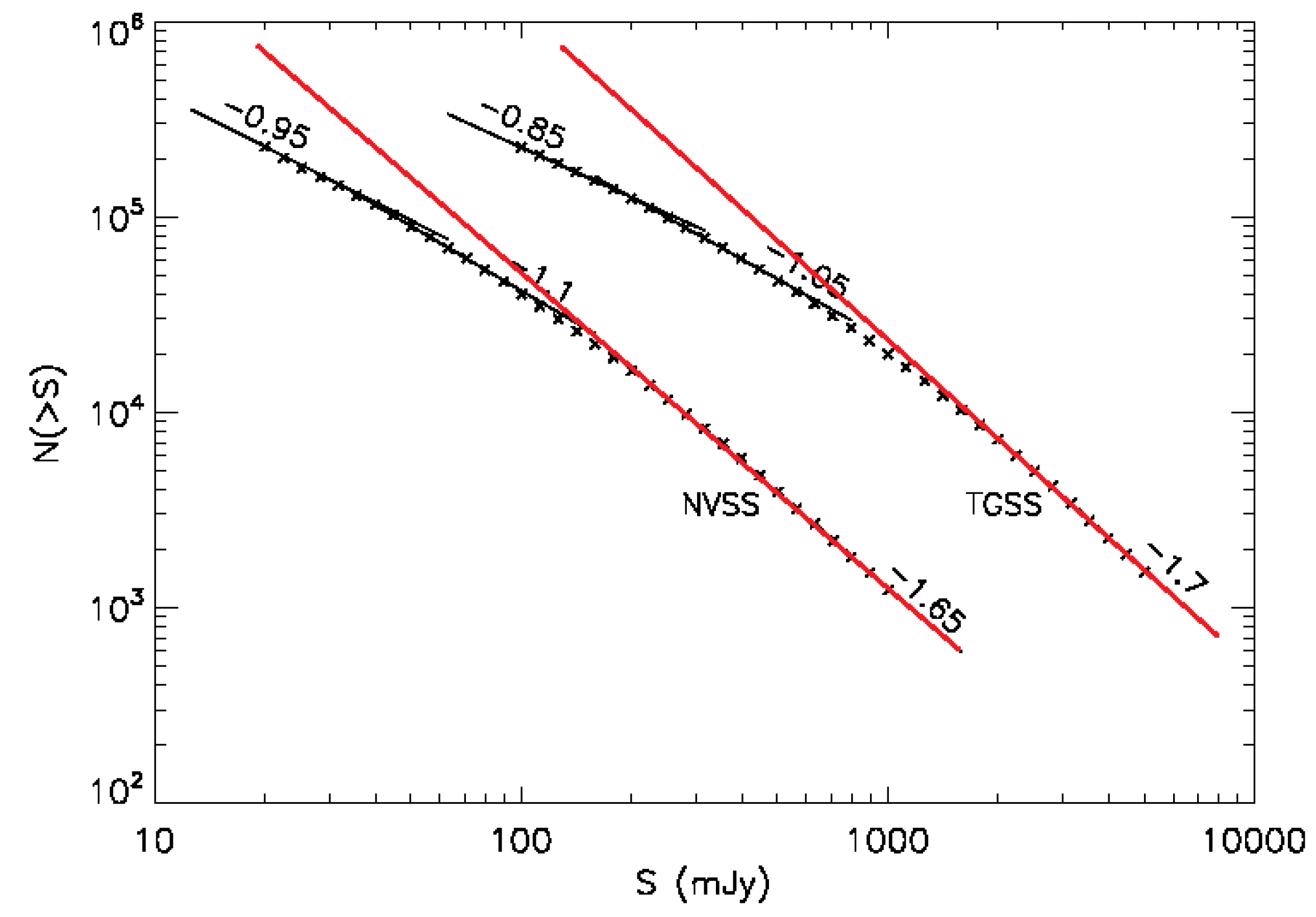
We find the answer to that question in the count versus flux level curves shown in Figure 5.
One of the basic premises of the EB model is that the galaxy counts obey the power-law distribution, Equation (12) with a constant value of x over a range of flux cutoff values. Looking at the curves in Figure 5, we see that they are not straight lines over the range of flux cutoffs considered in [3,4,5] but instead curve downward with source flux. The curves do approach straight lines but only for flux levels greater than about 300 mJy in the NVSS case and 2000 mJy in the TGSS case but these are well above the cutoffs used.
Equation (12) is considered to be a universal attribute of galactic structures but this assumes that the set of objects to which it is applied is in some sense pristine. In the current case, this can be interpreted to mean that the original population of radio galaxies dating back to the time of galaxy formation are all still with us and are all still emitting radiation. If that were the case, the counts would lie on the red lines. What seems to be happening, however, is that some of those radio galaxies are running out of fuel. They are still there but they no longer look like radio galaxies. The consequence is that the observed counts in the lower range of flux levels are less than what would be expected based on the universal law.
When making predictions, values of x and are inserted into the model equations so with curves having a varying slope for small flux levels, one can get any of a range of dipole predictions by shifting the flux cutoff and that is clearly wrong since there is only one dipole.
To fix the problem, all that is needed is to increase the flux cutoff into the range in which the curves of Figure 5 are straight lines. The lines from both datasets have the same slope, , which is close to the quasar value.
The spectral parameter, , might also be subject to a similar effect but we don’t have a set of curves to check that possibility. Using the existing value of , we find values of and which arewithin 20% of the quasar values. With this correction, the predicted dipole magnitudes for the quasars and the radio galaxies are essentially the same.
What remains is to re-analyze the radio galaxy datasets using the higher cutoffs given above. The difference between the quasar and radio galaxy measurements is already only about 20% and we expect that a re-analysis will reduce the difference even further.
There is still a difference between the NVSS and TGSS results to explain. The two curves are very similar with the same slopes but an order of magnitude difference in flux levels for any given count level, This would seem to indicate a calibration issue but that is for the experts to sort out. The dipole prediction, however, is only dependent on the slopes of the curves so both datasets result in the same predicted dipole.
We will now consider some possible contributors to the remaining 20%.
7. Reference Frame Consequences for the Spectra and Source Count Parameters
The rules of the game require that the selected set of observed objects must be isotropic in all aspects in the source frame and this clearly must apply to the spectral index , and the source count index, x.
Beginning with the spectral index, from the first equality of Equation (11), we have . (We have changed to indicate the spectral index is defined in the source frame.) In practice, the spectra are measured and parameterized in the observer frame using the same functional form so we have . Setting and solving for , we find . But so . Also, so we find that the difference between spectral indices measured in the two frames is very small and can be ignored. Next, the source count in the source frame is given by which is related to the count in the observer frame by . We now again suppose that the same functional form is applied in the observer frame so we have . If we scale by a common reference flux to make the equation dimensionless, for the same value of flux, we have so again, the correction is very small compared to the nominal value of the parameter.
8. Masking
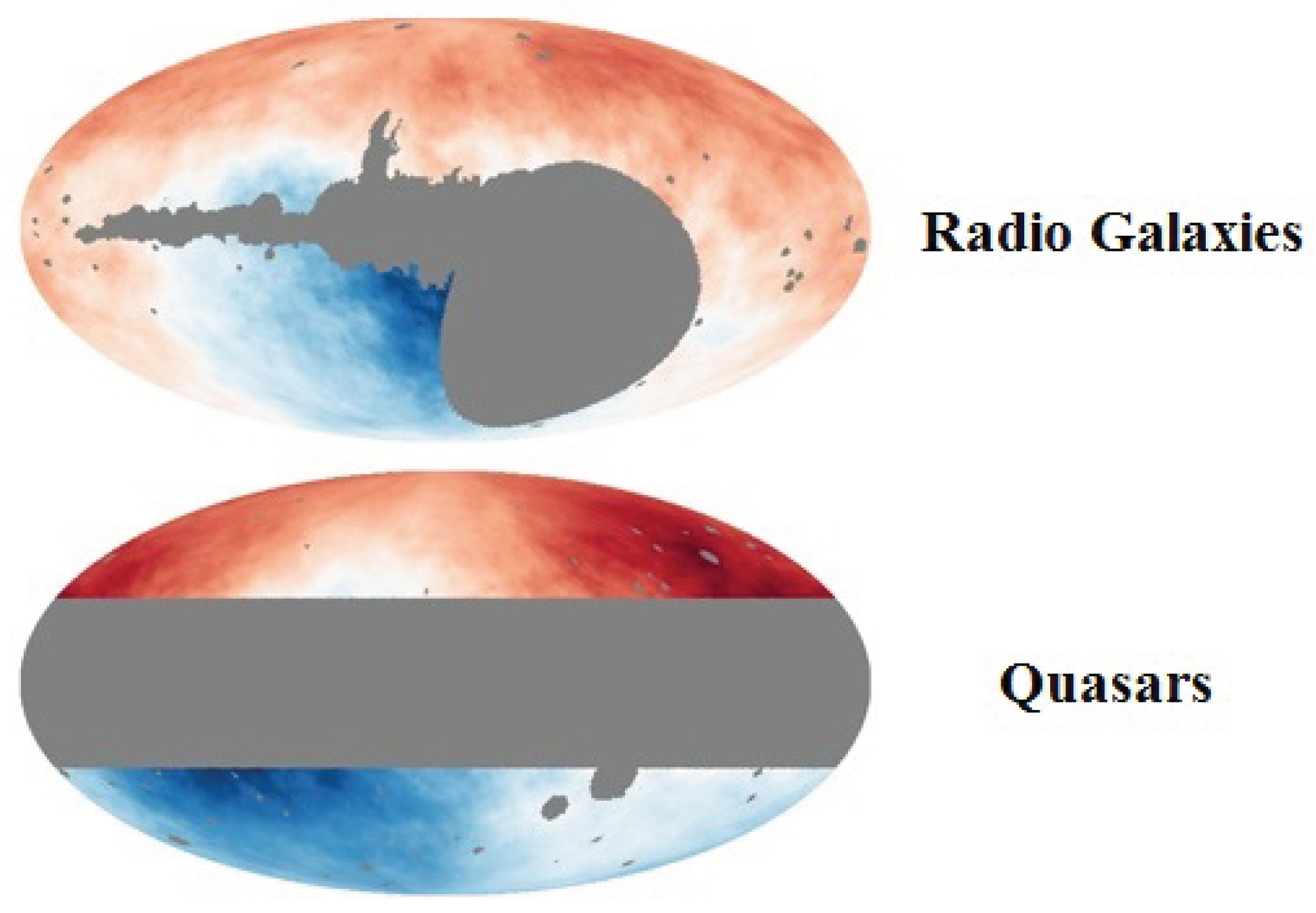
In Figure 6, we show the masking presently in use, [2,3,4,5]. The upper and lower figures show the radio galaxy and quasar masking respectively. Part of the 20% could be a consequence of masking bias because of the unfortunate fact that the dipole axis lies close to the galactic plane.
First, we will deal with the reference frame issue. Because of aberration, there is a distortion of any mask defined in one frame when viewed in the alternate frame with a magnitude proportional to . If one defines, for example, a uniform galactic mask in the source frame which would avoid bias, that mask would be pinched in the forward direction of the dipole and expanded in the backward direction in the observer frame. Conversely, a mask defined in the observer frame would be distorted in the opposite sense in the source frame. The result is that a mask defined in the observer frame introduces a bias in the dipole determination unless accounted for by a redefinition of the observer frame mask. The same distortion occurs for any mask so one must consider the consequences of aberration in each case.
The published studies are based on galaxy collections containing up to 1 million objects but the reality is that most of those contribute very little to the dipole determination because they are too far from the axis. On the other hand, of the small percentage that lie close to the ends of the dipole axis, and which contribute the most to its determination, a significant portion are hidden from view by the masking. This is particularly true in the radio galaxy case because the masking is highly asymmetric with the large asymmetry lying almost on top of the dipole axis in the lower hemisphere without a corresponding mask near the upper end of the axis.
The best one can do to extract the most information from the existing galaxy counts is to run simulations to assess the impact of the various masks but in such simulations, the masks should be defined in the source frame and then boosted to the observer frame to minimize the aberration bias.
9. Motion of the Earth
Generally, researchers speak of our peculiar velocity dipole in terms of the motion of the Solar system but we are not at rest in that system. To assess the importance of the motions, we need to determine both the relative magnitude of those motions with respect to the magnitude of the peculiar velocity, and the orientation of those motions with respect to the dipole axis. For the latter, the direction of the CMB dipole is in galactic coordinates which becomes in the ecliptic plane from which we determine the important fact that, for practical purposes, the dipole axis lies in the orbital plane of the Earth.
There are three significant motions to consider. The equatorial surface speed of the Earth is which is very much smaller than the peculiar velocity so the rotation of the Earth about its axis can be ignored.
Next, observations are made from Earth orbit satellites and these have speeds in the range of 3.1 to which are larger but still small compared to the peculiar velocity. These motions also have relatively short periods so there would be considerable averaging during the timespan of individual observations. The consequence will be some smearing of the results but not by more than a few percent.
The orbital motion of the earth, however, is another matter because the orbital speed is which is 8.1% of the average peculiar velocity. This, by itself, would not matter but we also know that the dipole axis lies in the same plane. This consequence is that the instantaneous peculiar velocity varies between and sinusoidally during the year.
During the year some galaxies would be dropping below the flux cutoff during one part of the year and rising above it during the remainder so this is not a small matter since it leads to a significant systematic error which, as far as we call tell, has been overlooked. This issue is certainly not mentioned in the papers we have been discussing. The variation would have a significant effect on the error estimates but even more to the point, depending on the scanning protocol of either ground-based or satellite observations, a systematic scanning of one region of the sky during one season and another region during a different season could result in a significant false bias in number counts which could be interpreted as an inhomogeneous distribution of matter across the sky. This would be particularly the case with ground-based optical observations since they can only be made at night. The result would be a false bias in the number counts in each region of the sky that would be repeated year after year making the error appear as an actual inhomogeneity.
10. Conclusions
We have shown that correcting the analysis used to predict the matter dipole eliminates almost all the difference between the model predictions and the measured values. The remaining differences are on the order of 20%.
We have considered possible contributors to that 20% but it doesn’t appear likely that they can account for much of the 20%. It appears more likely that much of the remaining difference is a consequence of actual large-scale inhomogeneities of matter in the universe. It is important to appreciate that such excesses have no bearing on the actual dipole which is almost certainly solely a consequence of our peculiar velocity which is itself a consequence of local inhomogeneities. If we could turn off our peculiar velocity, the dipole would disappear but the inhomogeneities would remain albeit with magnitudes an order of magnitude smaller than expected based on the published estimates of the dipole excess.
While such large-scale inhomogeneities would present a problem for the ΛCDM model, such inhomogeneities are predictions of new models of cosmology that propose a fractal origin of all cosmic structures. One of the defining properties of a fractal system is scale invariance and the power-law empherical formulas, Equations (10) and (12), are themselves an indication of such a universe. In our new model, [9,10,11], for example, fractal structures on all length scales are expected. In this model, the universe began with a Planck-era inflation involving only the vacuum. The vacuum or more particularly the vacuum energy that came into existence was homogeneous and isotropic aside from a small amplitude fractal imprint that later regulated the creation of ordinary matter at the time of nucleosynthesis. It is the vacuum that expresses the notion of a cosmological principle directly while the matter only expresses the cosmological principle on a statistical basis. The meaning of that is that the probability of finding matter in some region of space has a uniform distribution but the realization of the matter has a highly non-homogeneous fractal distribution. At a time of about , a fraction of about of the vacuum energy converted into neutron/antineutron pairs [12] with a very small excess of neutrons via a process that was regulated by the fractal imprint. One prediction of the model that is relevant to the present discussion is that the CMB radiation with its anisotropies [13,14] and the matter content of the universe including the structures were the outcome of a single event and so must have the same rest frame. Subsequently, aside from local peculiar motion, the matter hasn’t moved. We are still sitting at nearly the same spot in the universe that we occupied at the time of nucleosynthesis. The CMB radiation, on the other hand, has been dispersing around the universe ever since which accounts for its near isotropy.
In conclusion, we first identified the errors that are responsible for a major portion of the excess magnitudes of the quasar and radio galaxy dipoles reported in all previous studies. We show that the correct treatment of the source flux cutoff issue removes about 80% of the excess in the quasar case and about 30% of the published excess in the radio galaxy case. We then show that increasing the flux cutoff in the radio galaxy case eliminates essentially all the remaining difference between the quasar and radio galaxy predictions.
Funding
No funding was received for this research.
Institutional Review Board Statement
This manuscript has no associated code/software.
Data Availability Statement
Data sharing not applicable - no new data generated.
Conflicts of Interest
The author declares no conflicts of interest.
References
- Perivolaropoulos, L.; Skara, F. Challenges for ΛCDM: An update. ArXiv 2022, 2105.05208v3. [Google Scholar] [CrossRef]
- Secrest, N.J.; et al. A Test of the Cosmological Principle with Quasars. apjl 2021, 908, L51. [Google Scholar] [CrossRef]
- Secrest, N.J.; et al. A Challenge to the Standard Cosmological Model. apjl 2022, 937, L31. [Google Scholar] [CrossRef]
- Singal, A.K. Large Peculiar Motion fo the Solar System From the Dipole Anisotropy in Sky Brightness Due to Distant Radio Sources. apjl 2011, 742, L23. [Google Scholar] [CrossRef]
- Singal, A.K. A large disparity in cosmic reference frames determined from the sky distributions of radio sources and the microwave background radiation. Phys. Rev. D 2019, 100, 063501. [Google Scholar] [CrossRef]
- Ellis, G.F.R.; Baldwin, J.E. On the expected anisotropy of radio source counts. mnras 1984, 206, 377–381. [Google Scholar] [CrossRef]
- Rieger, F. High Energy Astrophysics - Lecture 3, 3. https://www.mpi-hd.mpg.de/personalhomes/frieger/HEA3.pdf, https://doi.org/https://www.mpi-hd.mpg.de/personalhomes/frieger/HEA3.pdf.
- Rieger, F. High Energy Astrophysics - Lecture 4, 4. https://www.mpi-hd.mpg.de/personalhomes/frieger/HEA4.pdf, https://doi.org/https://www.mpi-hd.mpg.de/personalhomes/frieger/HEA4.pdf.
- Botke, J.C., Cosmology with Time-Varying Curvature: A Summary. In Cosmology - The Past, Present and Future of the Universe; 2023; pp. 69–105. [CrossRef]
- Botke, J.C. A Different Cosmology: Thoughts from Outside the Box. Journal of High Energy Physics, Gravitation and Cosmology 2020, 6, 473–566. [Google Scholar] [CrossRef]
- Botke, J.C. Thoughts on the Origin of our Fractal Universe. Journal of Modern Physics 2025, 8, 167–197. [Google Scholar] [CrossRef]
- Botke, J.C. The Origin of Cosmic Structure, Part 4 – Nucleosynthesis. Journal of High Energy Physics, Gravitation and Cosmology 2022, 8, 768–799. [Google Scholar] [CrossRef]
- Botke, J.C. The Origin of Cosmic Structure, Part 6 – CMB Anisotropy. Journal of High Energy Physics, Gravitation and Cosmology 2024, 10, 257–276. [Google Scholar] [CrossRef]
- Botke, J.C. The Reality of Baryonic Acoustic Oscillations. Journal of Modern Physics 2024, 15, 375–400. [Google Scholar] [CrossRef]
Figure 1.
Uniform flux cutoff in the source rest frame.
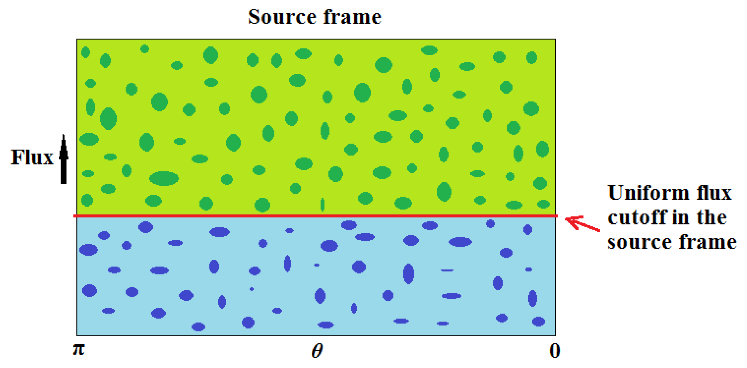
Figure 2.
The galaxies of Figure 1 boosted to the observer rest frame.
Figure 2.
The galaxies of Figure 1 boosted to the observer rest frame.
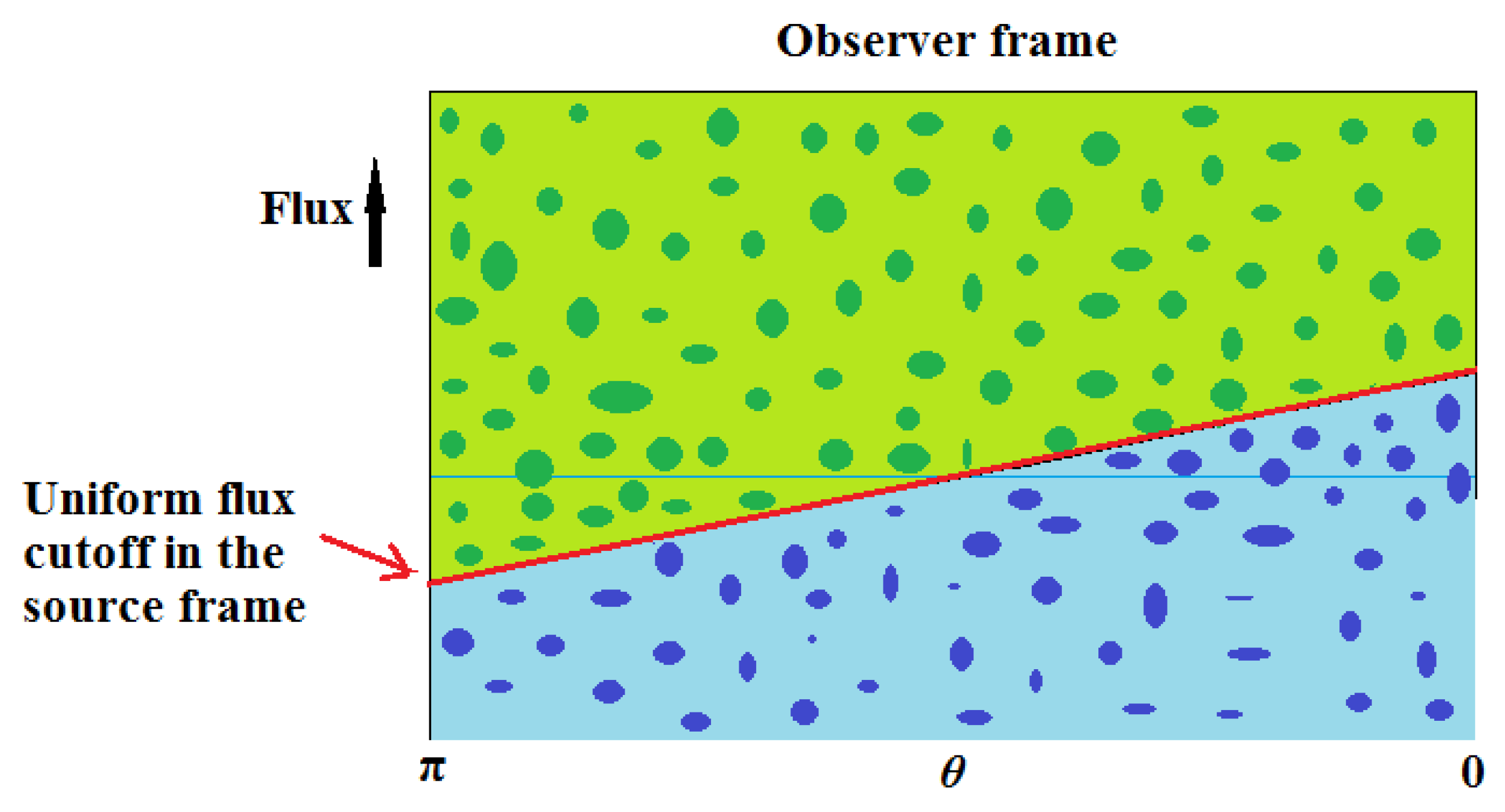
Figure 3.
Still the observer rest frame but now showing a uniform flux cutoff in the observer frame.
Figure 3.
Still the observer rest frame but now showing a uniform flux cutoff in the observer frame.
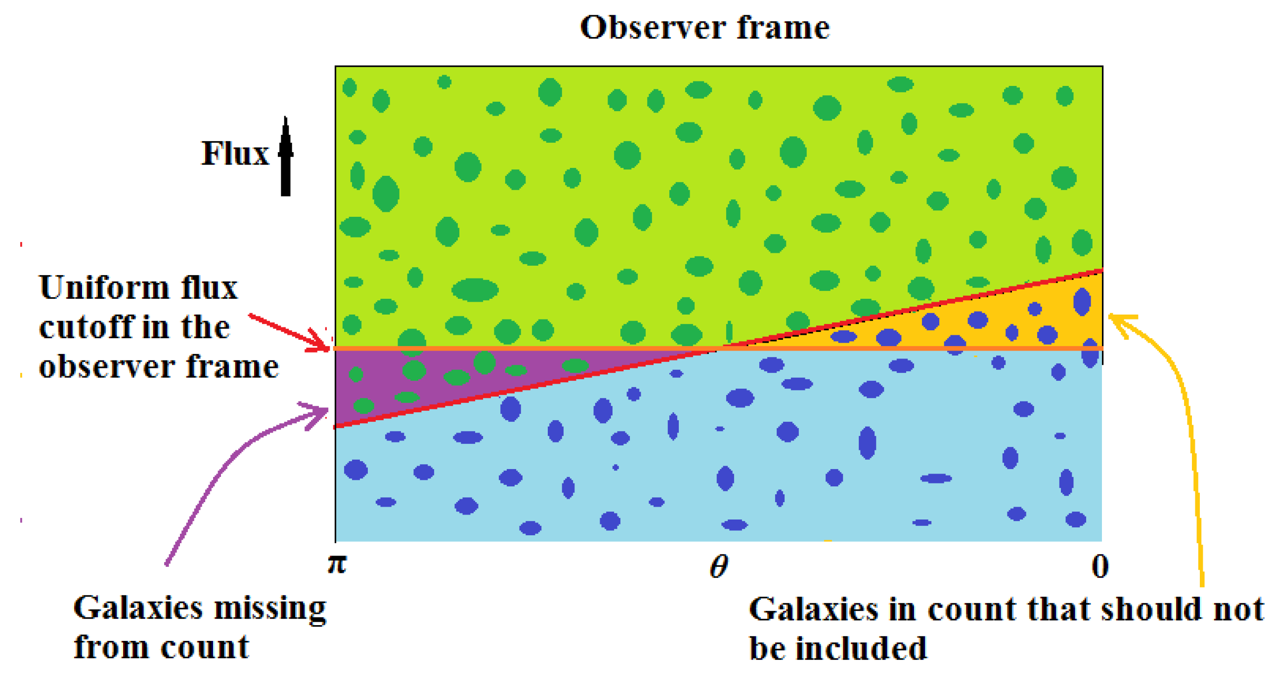
Figure 4.
Back in the source rest frame.
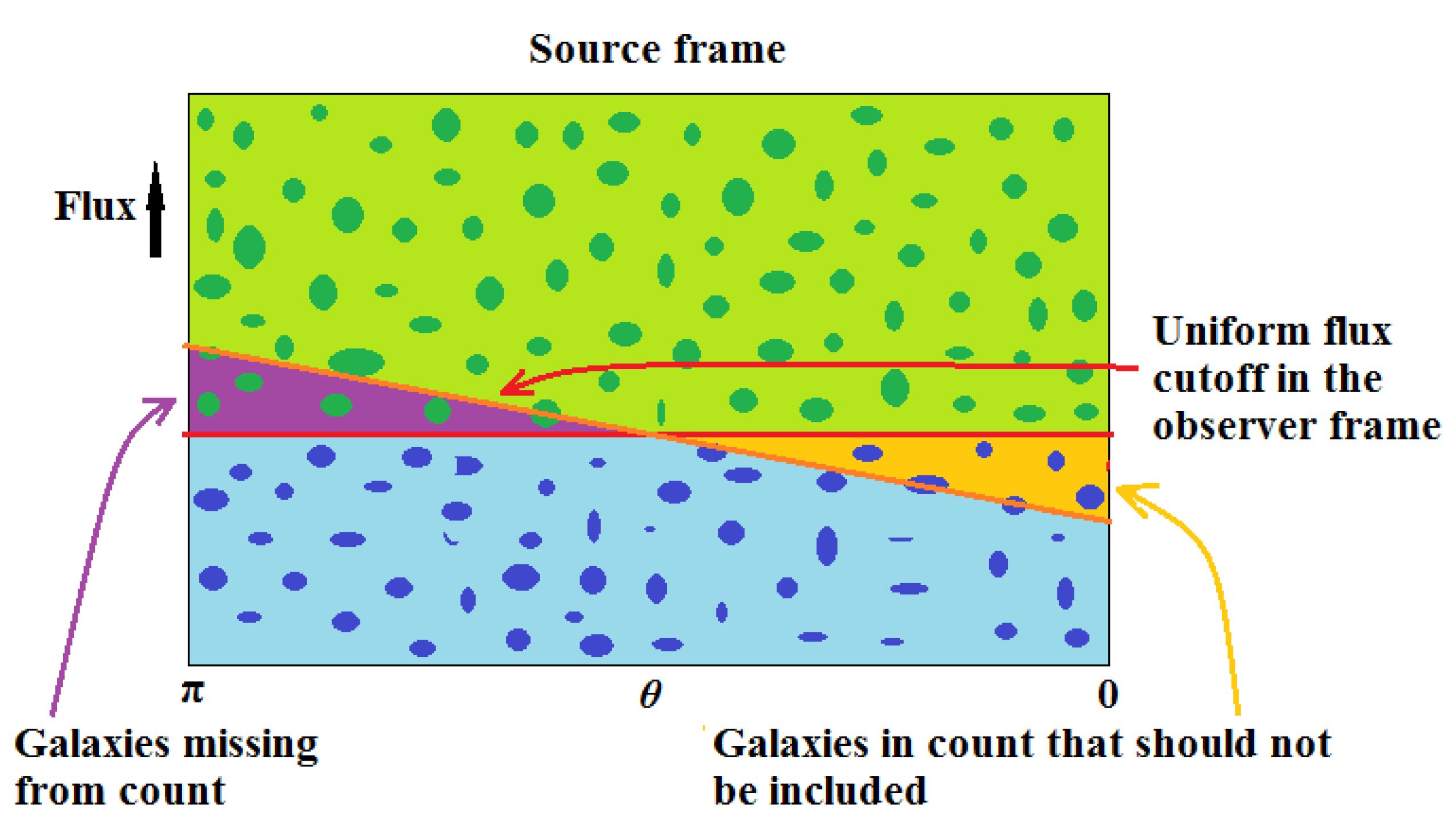
Figure 5.
Plot of the count of galaxies per solid angle versus source flux for both the NVSS and TGSS radio galaxy datasets. (Adaptation of Figure 1 of [5].)
Disclaimer/Publisher’s Note: The statements, opinions and data contained in all publications are solely those of the individual author(s) and contributor(s) and not of MDPI and/or the editor(s). MDPI and/or the editor(s) disclaim responsibility for any injury to people or property resulting from any ideas, methods, instructions or products referred to in the content. |
© 1996 by the author. Licensee MDPI, Basel, Switzerland. This article is an open access article distributed under the terms and conditions of the Creative Commons Attribution (CC BY) license (https://creativecommons.org/licenses/by/4.0/).
Copyright: This open access article is published under a Creative Commons CC BY 4.0 license, which permit the free download, distribution, and reuse, provided that the author and preprint are cited in any reuse.


