
Submitted:
11 October 2025
Posted:
13 October 2025
You are already at the latest version
Abstract
Forests at the urban–mountain interface moderate local climate, yet the spatial coupling between thermal regimes and vegetation dynamics is not well quantified. Focusing on Namyangju (Republic of Korea), we analyzed eight cloud-free Landsat-8/9 scenes from 2023 over forested pixels (30 m). Land surface temperature (LST) was retrieved from Lev-el-1 thermal Band 10, and NDVI from Bands 4–5. For each pixel we computed annual co-efficients of variation (CV) for LST and NDVI, then applied Getis–Ord Gi* to derive Z-scores (GiZ) that identify statistically significant clusters of intra-annual variability. We compared two formulations of the LST–NDVI linkage across ~308,000 grid points: regres-sion of variability magnitudes (CV–CV) and regression of local clustering intensities (GiZ–GiZ). Both relationships were positive, but GiZ–GiZ exhibited a tighter fit (R² = 0.623) than CV–CV (R² = 0.464), indicating stronger co-location of thermal and greenness clusters than raw variability alone suggests. Hotspots for both fields coincided with upland ridges and dissected slopes, whereas coldspots concentrated in valleys, highlighting terrain’s first-order control on microclimate and phenology. Methodologically, coupling time-series CVs with Gi* and simple OLS on GiZScores provides a transparent, spatially informed indicator of thermal–greenness coupling. Practically, GiZ-based belts offer actionable tar-gets for monitoring and management in urban-adjacent forests.
Keywords:
Land Surface Temperature
; NDVI
; Hotspot Analysis
1. Introduction
Forests identified in land-cover maps are increasingly recognized as a Nature-based Solution (NBS) that moderates climate through tree-dominated processes [1,2,3]. In particular, forest canopies buffer energy exchange between the atmosphere and the land surface and regulate surface temperature via radiative shielding and evapotranspiration, thereby playing a pivotal role in maintaining local climate stability [4,5,6]. Forests also store atmospheric carbon dioxide (CO₂) in biomass, reducing greenhouse gases (GHGs) and mitigating climate change. These functions position forests, within the NBS framework, as critical natural capital that delivers both mitigation and adaptation [7,8,9,10]. Sustaining these NBS benefits requires continuous, wall-to-wall monitoring and adaptive forest management. [11,12,13]. However, approximately 63% of South Korea is forested, making comprehensive field surveys across the entire territory impractical [14,15]. To overcome this constraint, the forest sector increasingly relies on remote sensing for synoptic, repeatable, and spatially explicit monitoring beyond sample-based assessments.
To operationalize monitoring of these NBS functions, we employ remote-sensing indicators that jointly capture canopy condition and surface thermal states—most notably the normalized difference vegetation index (NDVI) and land surface temperature (LST). The NDVI is a canonical observation-derived index that quantifies vegetation activity and cover [16,17]. Generally, higher NDVI indicates denser and healthier vegetation, supporting observation-based monitoring [18,19,20]. Land Surface Temperature (LST) is derived from thermal-infrared emissive properties to estimate surface temperature [21,22]. LST enables monitoring of thermal-related phenomena such as urban heat islands, drought, and crop or vegetation stress [23,24,25]. Both NDVI and LST can be obtained from satellite observations at commensurate acquisition times, for example from the United States Geological Survey (USGS) Landsat series [26,27]. NDVI and LST are tightly coupled: in summer, areas with high NDVI typically exhibit lower LST because canopy shading and evapotranspiration depress surface temperatures, yielding a negative association; in winter, the relationship can invert and become positive [28,29,30,31,32]. These seasonal reversals, driven by acquisition timing and phenology, are a critical consideration for data use [18,33,34,35], especially in strongly seasonal climates such as South Korea, where phenological dynamics render the NDVI–LST association non-stationary throughout the year.
Accordingly, treating the NDVI–LST relationship as a single global correlation is inadequate; approaches that reflect spatiotemporal structure and variability are required. In forested landscapes, both variables exhibit pronounced spatial autocorrelation, with similar values clustering among neighboring locations [36,37]. Conventional regression models that ignore this spatial structure can yield biased or misleading inferences, and mean-based statistics alone are ill-suited to capture such patterns. To characterize the spatial distribution of NDVI and LST more precisely, spatial statistics, particularly hotspot analysis capable of identifying local clusters, are warranted [38,39]. While hotspot analysis is informative, it is typically univariate, and thus additional procedures are needed to incorporate temporal variation.
This study addresses those limitations by integrating hotspot analysis with time-series statistics to elucidate the spatiotemporal relationship between LST and NDVI and, in turn, to explore forests’ climate-buffering function. We compute the annual coefficient of variation (CV) for time-series NDVI and LST and conduct hotspot analysis on these CV fields using Getis–Ord Gi* hotspot analysis [40,41]. The CV, a dimensionless ratio of the annual standard deviation to the mean, expresses fluctuation amplitude relative to the mean and thereby enables direct comparison of the relative variability of two variables with different units. We then assess their association by regressing the Getis–Ord Gi* Z-score (GiZScore) fields. In addition, we designate the upper 5% of the GiZScore distribution as “management-priority sites” and derive policy implications for spatially explicit forest management. Beyond purely numeric summary statistics, this framework provides a basis for understanding, in space and time, how forests respond to climate variability and for designing targeted responses.
This study offers decision-relevant evidence by analyzing NDVI–LST interactions across space and time and by objectively identifying forest areas where climate-mitigation and buffering functions are most pronounced. By overcoming limitations of conventional spatial analyses and leveraging simple transformations of readily available inputs, the approach proposes a new mode of using satellite-derived data with strong temporal dependence in seasonal regions such as South Korea.
2. Materials and Methods
2.1. Study Area
The study area is Namyangju, Gyeonggi-do, Republic of Korea (Figure 1). Situated on the eastern periphery of the Seoul Capital Region, Namyangju is an administrative district in which approximately 70% of the total area is forested, substantially higher than the provincial average of 52% [42]. This high forest fraction provides favorable conditions for evaluating the ecological and climatic functions that forests perform in urban-adjacent settings. Owing to its mosaic of urban fabric interspersed with forests, Namyangju is well suited to observe how multiple forest functions, including climate regulation, mitigation of urban thermal environments, and the provision of ecosystem services, are connected to everyday living spaces.
Additionally, Namyangju features steep slopes and mountainous terrain spanning a wide elevational range, making it well suited to analyze topographically driven spatial heterogeneity in vegetation and the attendant variation in land surface temperature. The area exhibits a mid-latitude continental climate with pronounced seasonal temperature contrasts, allowing observation of both summer heat and winter cold, which is advantageous for elucidating the seasonal relationship between LST and NDVI [43,44,45]. Among the relevant administrative units from which cloud-free, multi-temporal Landsat-8 and Landsat-9 imagery can be acquired to construct the time-series LST and NDVI inputs, including the neighboring, heavily forested jurisdictions of Pocheon and Yangpyeong, only Namyangju met the data-availability criteria for this study.
2.2. Datasets for Analysis
Both LST and NDVI are canonical observation-derived indices computed from satellite imagery. The two metrics respectively reflect the thermal state of the land surface and the vigor of vegetation activity. LST is retrieved from thermal-infrared radiance, typically by inverting a radiative transfer/Planck function to brightness temperature and then converting to land surface temperature with emissivity correction [46]. NDVI, defined from the contrast between red and near-infrared reflectance, captures vegetation density and condition [47]. Meaningful interpretation is enabled by comparing these datasets at coincident acquisition times and harmonized spatial resolution. Accordingly, quantifying the LST–NDVI relationship requires image data acquired by the same (or cross-calibrated) sensor platform. In this context, we used imagery from the Landsat-8 and Landsat-9 missions provided by the USGS.
The two satellites carry nearly identical and cross-calibrated payloads, Operational Land Imager (OLI/OLI-2) and Thermal Infrared Sensor (TIRS/TIRS-2), yielding high data continuity and interoperability [48]. OLI supplies the visible and near-infrared bands used to compute NDVI, while TIRS provides the thermal bands needed to estimate LST. Spatial sampling is 30 m for OLI, and 100 m (delivered resampled to 30 m) for TIRS, with each satellite on a 16-day repeat cycle; phased orbits provide ~8-day effective revisit when combined. For this study, we assembled eight cloud-free, multi-temporal Landsat-8/9 scenes over Namyangju during 2023; the acquired data are provided as Figure 2.
2.3. Data Processing
LST was retrieved from the thermal-infrared Band 10 of Landsat-8 and Landsat-9 Level-1 scenes, and NDVI was computed from the red (Band 4) and near-infrared (Band 5) bands. Although the USGS Level-2 product provides an LST layer, we found that the accompanying cloud mask was not adequate for our purposes and led to loss of valid observations across the time series. Accordingly, we derived both LST and NDVI directly from the Level-1 inputs.
To quantify the temporal stability and variability of LST and NDVI within forests, we spatially masked satellite scenes for Namyangju using the Ministry of Environment’s 2023 micro class land-cover map and retained only areas classified as “forest.” [49]. This restriction was intended to isolate and analyze climate–vegetation interactions specifically within forested landscapes.
Over the extracted forest mask, we generated a regular lattice of grid points at 30-m spacing, co-registered to the imagery and consistent with the native spatial resolution, yielding a total of 307,886 points. For each point, we extracted the complete time-series of LST and NDVI values for the study period. The resulting per-point series were then used to compute the mean, standard deviation (SD), and CV for each variable.
The CV, defined as SD divided by the mean, is a dimensionless measure that enables direct comparison of relative variability across variables with different units and ranges. Reliance on SD alone can over- or under-state variability as a function of absolute magnitude; introducing the CV mitigates this bias and provides a more interpretable basis for comparing the relative stability or sensitivity of LST and NDVI within forest areas.
We next performed hotspot analysis on the CV fields of LST and NDVI separately, using the Getis–Ord Gi* statistic and its standardized Z-score (GiZScore) to identify clusters of significantly high (hot) and low (cold) variability[40,41,50]. To assess the spatial coupling of variability between the two indices, we regressed the NDVI GiZScores on the LST GiZScores. The data flow of the study is summarized in Figure 3. Based on the hypothesis that areas with high thermal variability also experience elevated vegetation variability, we expected a positive regression coefficient. This analysis evaluates the strength and significance of that hypothesis at spatial scales relevant to management, providing evidence on how the forest climate-buffering function varies across space. In doing so, it empirically links thermal sensitivity and vegetation stability and offers spatially explicit information to support climate-adaptation and forest-management decision-making.
3. Results
3.1. Result of Getis–Ord Gi* Hotspot Analysis for CVs of LST and NDVI
The spatial distributions of hotspots in annual CV of LST and NDVI, derived via Getis–Ord Gi* hotspot analysis, are shown in Figure 4a, b. In both variables, the Getis–Ord Gi* maps of annual CV reveal a coherent spatial organization. Despite differences in the areal extent of clusters across confidence thresholds, LST and NDVI exhibit broadly congruent patterns: hotspots form continuous bands along high-elevation ridges and dissected mountain slopes, whereas coldspots dominate valley floors and low-lying terrain. The close correspondence with the digital elevation model (DEM) indicates that terrain imposes a first-order control on intra-annual variability (Figure 1b).
We delineated management-priority areas by selecting grid cells that simultaneously fell within the top 5% of Getis–Ord Gi* Z-scores for both LST CV and NDVI CV—i.e., locations where intra-annual thermal and greenness variability are each significantly clustered at or above the 95th percentile. Operationally, we intersected the two hotspot layers to isolate zones of co-clustered variability. Comparison with the DEM (Figure 1b) shows that these co-hotspot belts are preferentially situated in higher-elevation terrain, with elevation distributions shifted upward relative to the forest-wide baseline and spatial concentrations along upland ridges and dissected, steep slopes. This topographic alignment indicates that orographic controls—enhanced thermal contrasts, aspect-driven insolation, wind exposure, and thinner soils—coincide with stronger phenological amplitude and canopy structural heterogeneity, jointly amplifying both LST and NDVI variability. From a management standpoint, these high-elevation co-hotspots constitute priority surveillance and intervention zones for climate-adaptation actions.
In mountainous zones, stronger seasonal thermal contrasts, aspect-driven insolation gradients, wind exposure, thinner soils, and intermittent water limitation jointly amplify LST variability; concomitantly, phenological amplitude and canopy structural heterogeneity enhance NDVI variability. Conversely, valley bottoms—benefiting from hydrologic buffering, gentler slopes, and more continuous canopy cover—show relatively muted variability in both fields.
A few local mismatches between the two maps suggest partial decoupling of thermal and greenness dynamics. For example, LST hotspots extend more broadly than NDVI hotspots in some ridge–shoulder complexes, consistent with thermal variability not always translating into proportional changes in vegetation greenness (e.g., where evergreen cover, shading, or soil moisture mitigate phenological swings). Taken together, the patterns support our hypothesis that spatial clustering of thermal variability tends to co-occur with clustering of vegetation variability, especially in complex terrain, and they identify upland belts as priority zones for monitoring climate–vegetation sensitivity.
3.2. Quantification of LST–NDVI Linkage Using Ordinary Least Squares
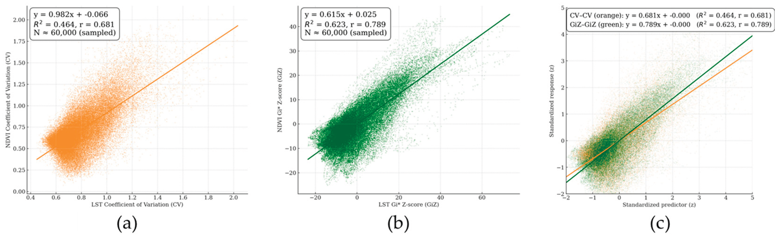
We estimated two ordinary least squares (OLS) specifications to quantify the LST–NDVI linkage across 307,886 forest grid points: (i) a variability model relating the coefficients of variation (CV–CV) and (ii) a hotspot model relating the Getis–Ord Gi* Z-scores (GiZ–GiZ), in each case regressing NDVI on LST. The CV specification yielded NDVI_CV = 0.982 × LST_CV − 0.066 with R² = 0.464 (Pearson r = 0.681), indicating a moderate–strong positive association in relative variability. The hotspot specification produced NDVI_GiZ = 0.615 × LST_GiZ + 0.025 with R² = 0.623 (Pearson r = 0.789), demonstrating a substantially tighter fit and stronger spatial concordance. Rank-based (Spearman) correlations showed the same ordering, confirming that the advantage of the hotspot formulation is not driven by a few extreme observations (Figure 5a, b). Interpreting the slopes, a one-unit increase in the LST GiZScore (i.e., one standard-unit increase in local clustering intensity of thermal variability) is associated with a ~0.62-unit increase in the NDVI GiZScore, consistent with co-located clusters of thermal and greenness variability (Figure 4a, b).
To facilitate direct visual comparison of the two relationships, we standardized each variable to z-scores (mean 0, standard deviation 1) and overlaid the CV–CV and GiZ–GiZ pairs in a single panel with identical axes. Specifically, both axes in Figure 5c are constrained to [−2, 5] and use a 1:1 scale; CV–CV is plotted in orange and GiZ–GiZ in dark green, with OLS lines drawn over point clouds. This normalization removes unit and scale effects, allowing the slopes to be interpreted purely as standardized effect sizes. Consistent with the regression results, the GiZ–GiZ line exhibits a steeper standardized slope than the CV–CV line, visually reinforcing that local clustering of thermal variability co-occurs more strongly with local clustering of vegetation variability.
We regard the GiZ-based formulation as the more appropriate representation of the LST–NDVI relationship. GiZScores are standardized local cluster statistics that explicitly incorporate neighborhood structure through a spatial weights matrix W. This construction reduces sensitivity to pixel-level noise (e.g., residual cloud shadow, geolocation jitter) and mitigates variance heterogeneity induced by spatial non-stationarity (e.g., terrain-driven shifts in local means and variances). As a result, the GiZ–GiZ regression yields a clearer and more stable signal of spatial co-clustering—the phenomenon of primary interest in this study—than a regression on raw CVs. Put differently, whereas CV–CV models can be confounded by large-scale gradients (elevation, aspect, soil moisture) that inflate or depress variability in different subregions, the GiZ transformation benchmarks each location against its local context, thereby sharpening the inferential contrast between hot and cold belts of joint variability.
For these reasons, we adopt the GiZ–GiZ OLS as our primary indicator and interpret it as a statistical characterization of the spatial association between thermal and greenness dynamics. We did not fit additional spatial-lag or spatial-error regressions because the GiZ transformation already embeds key spatial features, local averaging, standardization, and neighbor weighting, into the dependent and independent variables. This parsimonious approach avoids over-parameterization while directly targeting the mechanism of interest: the co-location of hotspots and coldspots in LST and NDVI.
4. Discussion
This study demonstrates that spatiotemporal clustering of thermal variability (LST CV) is closely mirrored by clustering of vegetation variability (NDVI CV) across a mountainous, forest-dominated urban fringe. The Getis–Ord Gi* results show that hotspots of intra-annual variability align with high-elevation ridges and dissected slopes, whereas coldspots concentrate in valley floors. This concordance with topography indicates that terrain imposes a first-order control on both thermal dynamics and phenology: stronger seasonal thermal contrasts, aspect-driven insolation gradients, wind exposure, and thinner soils in uplands amplify LST fluctuations; simultaneously, phenological amplitude and canopy structural heterogeneity increase NDVI variability. Conversely, hydrologically buffered lowlands with gentler slopes exhibit muted variability in both fields. Together, these patterns support the interpretation of forests as climate buffers whose effectiveness varies systematically with terrain and landscape position [51,52,53].
A key contribution of this study is the comparison between two ways of formalizing the LST–NDVI linkage using observation based remote sensing data: a direct regression of variability magnitudes (CV–CV) and a regression of local clustering intensities (GiZ–GiZ) [29,54,55]. Although both specifications yielded positive and statistically meaningful associations, the hotspot formulation provided a substantially tighter fit (R² = 0.623 vs. 0.464) and stronger rank concordance. We attribute this improvement to the properties of GiZScores: as standardized local statistics that explicitly embed neighborhood structure via a spatial weights matrix, GiZScores benchmark each pixel against its neighbors, attenuating pixel-scale noise and reducing variance heterogeneity caused by spatial non-stationarity[56,57]. In practical terms, the GiZ–GiZ model targets the phenomenon of interest—the co-location of thermal and greenness hotspots/coldspots—more directly than CV–CV and therefore serves as a more appropriate indicator of spatial coupling in complex terrain [58,59].
These findings carry several implications for forest monitoring and management in urban-adjacent mountain regions. First, the co-clustering of high thermal and high greenness variability in uplands suggests that upland belts function as sensitivity zones where climate anomalies are more likely to propagate into pronounced phenological responses [60,61,62]. Second, because our GiZ approach identifies statistically concentrated belts rather than isolated pixels, it can inform operational prioritization—for example, targeting the top 5% of GiZScores as “management-priority sites” for intensified field checks, fuel-load management, microclimate restoration (e.g., windbreaks, understory moisture conservation), or the placement of in situ temperature/soil-moisture loggers. Third, the persistence of coldspots in valley floors highlights the role of hydrological buffering; safeguarding riparian corridors and cold-air drainage pathways may help maintain local thermal stability and phenological regularity within the broader urban matrix.
Methodologically, the study contributes a parsimonious yet spatially informed pipeline for coupling time-series variability metrics with local cluster statistics. Computing annual CVs provides a unitless, comparable measure of intra-annual fluctuation; applying Gi* to the CV fields transforms those fluctuations into statistically vetted clusters; and a simple OLS on GiZScores yields an interpretable slope (co-clustering strength) without resorting to heavily parameterized spatial-lag or spatial-error models [63,64]. We deliberately did not fit SAR/SEM/SDM models because the GiZ transformation already embeds key spatial features—local averaging, standardization, and neighbor weighting—into both the predictor and response, thereby mitigating spatial dependence at the modeling stage while keeping the analysis transparent and reproducible. In settings where explicit process-based spatial spillovers are hypothesized (e.g., fire spread), spatial regression would remain valuable; however, for co-clustering of variability, GiZ–GiZ OLS strikes a favorable balance between robustness and simplicity.
This study has four main limitations. (1) Temporal scope—analyses are limited to a single year (2023), so interannual stability and trends remain to be tested. Additionally, satellite imagery from the summer season (June to August) was unavailable. This is because, due to the extreme cloud cover characteristic of Korea's climate, images with no cloud cover were excluded during the screening process. Therefore, strictly speaking, this does not cover all phenolgy for the entire year. (2) LST retrieval uncertainty—Level-1–based thermal estimates may retain emissivity and atmospheric correction errors and warrant in situ validation. (3) Index choice—NDVI saturation can limit sensitivity in dense canopies; alternative or complementary indices (e.g., Enhanced vegetation index (EVI), red-edge, Solar-induced chlorophyll fluorescence (SIF)) should be evaluated. (4) Neighborhood design—GiZ outcomes depend on the spatial weights matrix and neighborhood size. Future work can address these by extending to multi-year datasets, refining LST retrievals with ground truth, testing additional vegetation indices, and conducting sensitivity and multiple-testing assessments.
From a policy perspective, integrating GiZ-based hotspot belts into municipal forest plans could help align routine surveillance with areas of greatest climate–vegetation sensitivity. Because the method is sensor-agnostic and computationally light, it is readily transferable to other counties in Gyeonggi-do and to other seasonal, mountainous regions where rapid, wall-to-wall screening is needed. More broadly, mapping the spatial concordance of thermal and phenological variability provides an observation-based line of evidence for climate-buffering by forests, supporting nature-based solutions in local climate-adaptation and carbon-neutrality strategies [65,66].
In sum, by combining time-series variability metrics with standardized local clustering, this study provides a statistically grounded yet operationally usable view of how forests modulate microclimate across complex terrain. The stronger performance of the GiZ formulation underscores the value of explicitly leveraging neighborhood structure when translating pixel-level satellite observations into management-relevant insights about spatial coupling between thermal regimes and vegetation dynamics.
5. Conclusions
This study shows that intra-annual thermal variability (LST CV) and vegetation variability (NDVI CV) co-cluster systematically in mountainous, forested urban fringes, with hotspots aligned to upland ridges and coldspots concentrated in valleys. By pairing time-series variability metrics with Getis–Ord Gi* hotspot statistics, we quantified not only the magnitude of variability but also its spatial organization. Regressions confirmed a positive LST–NDVI linkage in both formulations, with the GiZ–GiZ specification yielding a substantially tighter fit than CV–CV, indicating that local clustering of thermal dynamics more strongly co-occurs with clustering of greenness dynamics than raw variability alone would suggest.
Methodologically, the workflow—annual CV computation → Gi* hotspot mapping → OLS on GiZScores—offers a transparent, lightweight, and spatially informed alternative to heavily parameterized spatial models. Because GiZScores embed neighborhood structure via the spatial weights matrix, they mitigate pixel-scale noise and variance heterogeneity, producing an interpretable slope that directly indexes co-clustering strength. The standardized overlay (Figure 3) further demonstrates, on a common scale, the stronger standardized slope for GiZ–GiZ, reinforcing the spatial coupling between thermal and phenological variability.
Practically, these results support using GiZ-based hotspot belts to prioritize monitoring and intervention in upland “sensitivity zones,” while recognizing valley coldspots as hydrologically buffered areas that stabilize local microclimate. The approach is sensor-agnostic, computationally efficient, and readily transferable to other seasonal, mountainous regions, making it suitable for routine, wall-to-wall screening in municipal forest plans and for integrating observation-based evidence into nature-based climate-adaptation and carbon-neutrality strategies.
Future work should generalize beyond a single year, refine thermal retrievals with ground validation, and test complementary vegetation indices (e.g., EVI, red-edge, SIF) to probe canopy dynamics more sensitively. Even so, the present findings provide decision-relevant evidence that explicitly leveraging neighborhood structure clarifies where and how forests buffer climate across complex terrain—turning pixel-level satellite signals into spatial intelligence for management.
Author Contributions
Conceptualization, J.K.; methodology, J.K.; software, J.K.; validation, J.K., M.K. and W.K.; formal analysis, J.K.; investigation, J.K.; resources, M.K.; data curation, J.K..; writing—original draft preparation, J.K.; writing—review and editing, W.K., M.K. and W.L.; visualization, J.K.; supervision, W.L.; project administration, M.K.; funding acquisition, M.K. All authors have read and agreed to the published version of the manuscript.
Funding
This work was supported by Korea Environment Industry & Technology Institute (KEITI) through “Climate Change R&D Project for New Climate Regime” grant number [RS-2022-KE002472] and “Creation and Management of Ecosystem-based Carbon Sinks” grant number [RS-2023-00218243], funded by the Ministry of Environment.
Data Availability Statement
The Landsat-8/9 data used in this study were obtained from the USGS. These data can be accessed through USGS Earth Explorer (https://earthexplorer.usgs.gov/). The forest mask used in this study was obtained from the Ministry of Environment of the Republic of Korea. These data can be accessed through the Environmental Spatial Information Service (https://egis.me.go.kr/).
Conflicts of Interest
The authors declare no conflicts of interest.
Abbreviations
The following abbreviations are used in this manuscript:
| NBS | Nature based solution |
| GHGs | Greenhouse gases |
| NDVI | Normalized difference vegetation index |
| LST | Land surface temperature |
| USGS | United States Geology Survey |
| CV | Coefficient of variation |
| OLI | Operational land imager |
| TIRS | Thermal infrared sensor |
| SD | Standard deviation |
| DEM | Digital elevation model |
| OLS | Ordinary least squares |
| EVI | Enhanced vegetation index |
| SIF | Solar-induced chlorophyll fluorescence |
References
- Zhao, J.; Davies, C.; Veal, C.; Xu, C.; Zhang, X.; Yu, F. Review on the Application of Nature-Based Solutions in Urban Forest Planning and Sustainable Management. Forests 2024, 15, 727. [Google Scholar] [CrossRef]
- Kong, X.; Zhang, X.; Xu, C.; Hauer, R.J. Review on Urban Forests and Trees as Nature-Based Solutions over 5 Years. Forests 2021, 12, 1453. [Google Scholar] [CrossRef]
- Bhattacharjee, A. Forest Landscape Restoration as a NbS Strategy for Achieving Bonn Challenge Pledge: Lessons from India’s Restoration Efforts. In Proceedings of the Nature-Based Solutions for Resilient Ecosystems and Societies; Springer: Singapore, 2020; pp. 133–147. [Google Scholar]
- Chen, J.; Saunders, S.C.; Crow, T.R.; Naiman, R.J.; Brosofske, K.D.; Mroz, G.D.; Brookshire, B.L.; Franklin, J.F. Microclimate in Forest Ecosystem and Landscape Ecology: Variations in Local Climate Can Be Used to Monitor and Compare the Effects of Different Management Regimes. BioScience 1999, 49, 288–297. [Google Scholar] [CrossRef]
- De Frenne, P.; Lenoir, J.; Luoto, M.; Scheffers, B.R.; Zellweger, F.; Aalto, J.; Ashcroft, M.B.; Christiansen, D.M.; Decocq, G.; De Pauw, K.; et al. Forest Microclimates and Climate Change: Importance, Drivers and Future Research Agenda. Glob Chang Biol 2021, 27, 2279–2297. [Google Scholar] [CrossRef]
- Hursh, C.R.; Connaughton, C.A. Effects of Forests Upon Local Climate. J For 1938, 36, 864–866. [Google Scholar] [CrossRef]
- Canadell, J.G.; Raupach, M.R. Managing Forests for Climate Change Mitigation. Science 2008, 320, 1456–1457. [Google Scholar] [CrossRef]
- Nunes, L.J.R.; Meireles, C.I.R.; Gomes, C.J.P.; Ribeiro, N.M.C.A. Forest Contribution to Climate Change Mitigation: Management Oriented to Carbon Capture and Storage. Climate 2020, 8, 21. [Google Scholar] [CrossRef]
- Locatelli, B.; Pavageau, C.; Pramova, E.; Di Gregorio, M. Integrating Climate Change Mitigation and Adaptation in Agriculture and Forestry: Opportunities and Trade-Offs. Wiley Interdiscip Rev Clim Change 2015, 6, 585–598. [Google Scholar] [CrossRef]
- Ravindranath, N.H. Mitigation and Adaptation Synergy in Forest Sector. Mitig Adapt Strateg Glob Chang 2007, 12, 843–853. [Google Scholar] [CrossRef]
- Kim, M.; Yoo, S.; Kim, N.; Lee, W.; Ham, B.; Song, C.; Lee, W.-K. Climate Change Impact on Korean Forest and Forest Management Strategies. Korean J. Environ. Biol. 2017, 35, 413–425. [Google Scholar] [CrossRef]
- Porté, A.; Bartelink, H.H. Modelling Mixed Forest Growth: A Review of Models for Forest Management. Ecol. Modell. 2002, 150, 141–188. [Google Scholar] [CrossRef]
- Camarretta, N.; Harrison, P.A.; Bailey, T.; Potts, B.; Lucieer, A.; Davidson, N.; Hunt, M. Monitoring Forest Structure to Guide Adaptive Management of Forest Restoration: A Review of Remote Sensing Approaches. New For. 2020, 51, 573–596. [Google Scholar] [CrossRef]
- Lee, J.; Lim, C.H.; Kim, G.S.; Markandya, A.; Chowdhury, S.; Kim, S.J.; Lee, W.K.; Son, Y. Economic Viability of the National-Scale Forestation Program: The Case of Success in the Republic of Korea. Ecosyst Serv 2018, 29, 40–46. [Google Scholar] [CrossRef]
- Kim, G.S.; Lim, C.H.; Kim, S.J.; Lee, J.; Son, Y.; Lee, W.K. Effect of National-Scale Afforestation on Forest Water Supply and Soil Loss in South Korea, 1971-2010. Sustainability 2017, 9. [Google Scholar] [CrossRef]
- Fung, T.; Siu, W. Environmental Quality and Its Changes, an Analysis Using NDVI. Int J Remote Sens 2000, 21, 1011–1024. [Google Scholar] [CrossRef]
- Pettorelli, N.; Vik, J.O.; Mysterud, A.; Gaillard, J.M.; Tucker, C.J.; Stenseth, N.C. Using the Satellite-Derived NDVI to Assess Ecological Responses to Environmental Change. Trends Ecol Evol 2005, 20, 503–510. [Google Scholar] [CrossRef]
- Kim, J.; Lim, C.H.; Jo, H.W.; Lee, W.K. Phenological Classification Using Deep Learning and the Sentinel-2 Satellite to Identify Priority Afforestation Sites in North Korea. Remote Sens 2021, 13. [Google Scholar] [CrossRef]
- Maselli, F. Monitoring Forest Conditions in a Protected Mediterranean Coastal Area by the Analysis of Multiyear NDVI Data. Remote Sens Environ 2004, 89, 423–433. [Google Scholar] [CrossRef]
- Kinyanjui, M.J. NDVI-Based Vegetation Monitoring in Mau Forest Complex, Kenya. Afr J Ecol 2011, 49, 165–174. [Google Scholar] [CrossRef]
- Li, Z.L.; Tang, B.H.; Wu, H.; Ren, H.; Yan, G.; Wan, Z.; Trigo, I.F.; Sobrino, J.A. Satellite-Derived Land Surface Temperature: Current Status and Perspectives. Remote Sens Environ 2013, 131, 14–37. [Google Scholar] [CrossRef]
- Neteler, M. Estimating Daily Land Surface Temperatures in Mountainous Environments by Reconstructed MODIS LST Data. Remote Sens 2010, 2, 333–351. [Google Scholar] [CrossRef]
- Holzman, M.E.; Rivas, R.; Piccolo, M.C. Estimating Soil Moisture and the Relationship with Crop Yield Using Surface Temperature and Vegetation Index. Int. J. Appl. Earth Obs. Geoinf. 2014, 28, 181–192. [Google Scholar] [CrossRef]
- Awais, M.; Li, W.; Hussain, S.; Cheema, M.J.M.; Li, W.; Song, R.; Liu, C. Comparative Evaluation of Land Surface Temperature Images from Unmanned Aerial Vehicle and Satellite Observation for Agricultural Areas Using In Situ Data. Agriculture 2022, 12, 184. [Google Scholar] [CrossRef]
- Kalma, J.D.; McVicar, T.R.; McCabe, M.F. Estimating Land Surface Evaporation: A Review of Methods Using Remotely Sensed Surface Temperature Data. Surv Geophys 2008, 29, 421–469. [Google Scholar] [CrossRef]
- Roy, D.P.; Wulder, M.A.; Loveland, T.R.; Woodcock, C.E.; Allen, R.G.; Anderson, M.C.; Helder, D.; Irons, J.R.; Johnson, D.M.; Kennedy, R.; et al. Landsat-8: Science and Product Vision for Terrestrial Global Change Research. Remote Sens Environ 2014, 145, 154–172. [Google Scholar] [CrossRef]
- Loveland, T.R.; Irons, J.R. Landsat 8: The Plans, the Reality, and the Legacy. Remote Sens Environ 2016, 185, 1–6. [Google Scholar] [CrossRef]
- Sun, D.; Kafatos, M. Note on the NDVI-LST Relationship and the Use of Temperature-Related Drought Indices over North America. Geophys Res Lett 2007, 34, L24406. [Google Scholar] [CrossRef]
- Karnieli, A.; Agam, N.; Pinker, R.T.; Anderson, M.; Imhoff, M.L.; Gutman, G.G.; Panov, N.; Goldberg, A. Use of NDVI and Land Surface Temperature for Drought Assessment: Merits and Limitations. J Clim 2010, 23, 618–633. [Google Scholar] [CrossRef]
- Marzban, F.; Sodoudi, S.; Preusker, R. The Influence of Land-Cover Type on the Relationship between NDVI–LST and LST-Tair. Int J Remote Sens 2018, 39, 1377–1398. [Google Scholar] [CrossRef]
- Guha, S.; Govil, H.; Diwan, P. Monitoring LST-NDVI Relationship Using Premonsoon Landsat Datasets. Adv. Meteorol. 2020, 2020, 4539684. [Google Scholar] [CrossRef]
- Taloor, A.K.; Parsad, G.; Jabeen, S.F.; Sharma, M.; Choudhary, R.; Kumar, A. Analytical Study of Land Surface Temperature for Evaluation of UHI and UHS in the City of Chandigarh India. Remote Sens Appl 2024, 35, 101206. [Google Scholar] [CrossRef]
- Kim, J.; Song, Y.; Lee, W.-K. Accuracy Analysis of Multi-Series Phenological Landcover Classification Using U-Net-Based Deep Learning Model-Focusing on the Seoul, Republic of Korea. Korean Journal of Remote Sensing 2021, 37. [Google Scholar] [CrossRef]
- Kim, J.; Jo, H.W.; Kim, W.; Jeong, Y.; Park, E.; Lee, S.; Kim, M.; Lee, W.K. Application of the Domain Adaptation Method Using a Phenological Classification Framework for the Land-Cover Classification of North Korea. Ecol Inform 2024, 81, 102576. [Google Scholar] [CrossRef]
- Kim, J.; Kim, W.; Lee, S.; Ko, Y.; Jeong, Y.; Lee, W.-K. Advancing Forest GHG Inventory Accuracy with a Phenological Classification Framework: Toward an Observation-Based Approach 3 in South Korea. Ecol Inform 2025, 91, 103420. [Google Scholar] [CrossRef]
- Zhang, X.; Hu, Y.; Zhuang, D.; Qi, Y.; Ma, X. NDVI Spatial Pattern and Its Differentiation on the Mongolian Plateau. J. Geogr. Sci. 2009, 19, 403–415. [Google Scholar] [CrossRef]
- Kowe, P.; Mutanga, O.; Odindi, J.; Dube, T. Exploring the Spatial Patterns of Vegetation Fragmentation Using Local Spatial Autocorrelation Indices. J Appl Remote Sens 2019, 13, 024523. [Google Scholar] [CrossRef]
- Kumar, S.; Parida, B.R. Hydroponic Farming Hotspot Analysis Using the Getis–Ord Gi* Statistic and High-Resolution Satellite Data of Majuli Island, India. Remote Sens. Lett. 2021, 12, 408–418. [Google Scholar] [CrossRef]
- Guerri, G.; Crisci, A.; Messeri, A.; Congedo, L.; Munafò, M.; Morabito, M. Thermal Summer Diurnal Hot-Spot Analysis: The Role of Local Urban Features Layers. Remote Sens (Basel) 2021, 13, 538. [Google Scholar] [CrossRef]
- Ord, J.K.; Getis, A. Local Spatial Autocorrelation Statistics: Distributional Issues and an Application. Geogr Anal 1995, 27, 286–306. [Google Scholar] [CrossRef]
- Getis, A.; Ord, J.K. The Analysis of Spatial Association by Use of Distance Statistics. Geogr Anal 1992, 24, 189–206. [Google Scholar] [CrossRef]
- Kim, H.; Lee, D.K. A Time-Series Analysis of Landscape Structural Changes Using the Spatial Autocorrelation Method-Focusing on Namyangju Area. J. Korea Soc. Environ. Restor. Technol. 2011, 3, 1–14. [Google Scholar]
- Natali, C.; Marchina, C.; Brombin, V.; Rahimi, E.; Dong, P.; Jung, C. Global NDVI-LST Correlation: Temporal and Spatial Patterns from 2000 to 2024. Environments 2025, 12, 67. [Google Scholar] [CrossRef]
- Guha, S. Dynamic Seasonal Analysis on LST-NDVI Relationship and Ecological Health of Raipur City, India. Ecosyst. Health Sustain. 2021, 7. [Google Scholar] [CrossRef]
- Guha, S.; Govil, H.; Taloor, A.K.; Gill, N.; Dey, A. Land Surface Temperature and Spectral Indices: A Seasonal Study of Raipur City. Geod Geodyn 2022, 13, 72–82. [Google Scholar] [CrossRef]
- Cristóbal, J.; Jiménez-Muñoz, J.C.; Prakash, A.; Mattar, C.; Skoković, D.; Sobrino, J.A. An Improved Single-Channel Method to Retrieve Land Surface Temperature from the Landsat-8 Thermal Band. Remote Sens (Basel) 2018, 10, 431. [Google Scholar] [CrossRef]
- Rouse, J.W., Jr.; Haas, R.H.; Schell, J.A.; Deering, D.W. Monitoring Vegetation Systems in the Great Plains with ERTS. In Proceedings of the 3rd ERTS-1 Symposium; NASA Goddard Space Flight Center: Washington, DC, USA, 1974; Volume 1, Section A; pp. 309–317. [Google Scholar]
- Xu, H.; Ren, M.; Lin, M. Cross-Comparison of Landsat-8 and Landsat-9 Data: A Three-Level Approach Based on Underfly Images. GIsci Remote Sens 2024, 61. [Google Scholar] [CrossRef]
- Ministry of Environment. Guidelines for Landcover Mapping; Ministry of Environment: Sejong, Republic of Korea, 2018. [Google Scholar]
- Jana, M.; Sar, N. Modeling of Hotspot Detection Using Cluster Outlier Analysis and Getis-Ord Gi* Statistic of Educational Development in Upper-Primary Level, India. Model Earth Syst Environ 2016, 2, 1–10. [Google Scholar] [CrossRef]
- Dobrowski, S.Z. A Climatic Basis for Microrefugia: The Influence of Terrain on Climate. Glob Chang Biol 2011, 17, 1022–1035. [Google Scholar] [CrossRef]
- Pepin, N.C.; Daly, C.; Lundquist, J. The Influence of Surface versus Free-Air Decoupling on Temperature Trend Patterns in the Western United States. J. Geophys. Res. Atmos. 2011, 116. [Google Scholar] [CrossRef]
- Lookingbill, T.R.; Urban, D.L. Spatial Estimation of Air Temperature Differences for Landscape-Scale Studies in Montane Environments. Agric For Meteorol 2003, 114, 141–151. [Google Scholar] [CrossRef]
- Guha, S.; Govil, H. An Assessment on the Relationship between Land Surface Temperature and Normalized Difference Vegetation Index. Environ Dev Sustain 2021, 23, 1944–1963. [Google Scholar] [CrossRef]
- Julien, Y.; Sobrino, J.A. Comparison of Cloud-Reconstruction Methods for Time Series of Composite NDVI Data. Remote Sens Environ 2010, 114, 618–625. [Google Scholar] [CrossRef]
- Peeters, A.; Zude, M.; Käthner, J.; Ünlü, M.; Kanber, R.; Hetzroni, A.; Gebbers, R.; Ben-Gal, A. Getis–Ord’s Hot- and Cold-Spot Statistics as a Basis for Multivariate Spatial Clustering of Orchard Tree Data. Comput Electron Agric 2015, 111, 140–150. [Google Scholar] [CrossRef]
- Rossi, F.; Becker, G. Creating Forest Management Units with Hot Spot Analysis (Getis-Ord Gi*) over a Forest Affected by Mixed-Severity Fires. Aust For 2019, 82, 166–175. [Google Scholar] [CrossRef]
- Anselin, L. Model Validation in Spatial Econometrics: A Review and Evaluation of Alternative Approaches. Int Reg Sci Rev 1988, 11, 279–316. [Google Scholar] [CrossRef]
- Cliff, A.D.; Ord, J.K. Spatial Processes: Models and Applications; Pion: London, UK, 1981. [Google Scholar]
- Jentsch, A.; Kreyling, J.; Boettcher-Treschkow, J.; Beierkuhnlein, C. Beyond Gradual Warming: Extreme Weather Events Alter Flower Phenology of European Grassland and Heath Species. Glob Chang Biol 2009, 15, 837–849. [Google Scholar] [CrossRef]
- De Frenne, P.; Zellweger, F.; Rodríguez-Sánchez, F.; Scheffers, B.R.; Hylander, K.; Luoto, M.; Vellend, M.; Verheyen, K.; Lenoir, J. Global Buffering of Temperatures under Forest Canopies. Nat Ecol Evol 2019, 3, 744–749. [Google Scholar] [CrossRef] [PubMed]
- Wolkovich, E.M.; Cook, B.I.; Allen, J.M.; Crimmins, T.M.; Betancourt, J.L.; Travers, S.E.; Pau, S.; Regetz, J.; Davies, T.J.; Kraft, N.J.B.; et al. Warming Experiments Underpredict Plant Phenological Responses to Climate Change. Nature 2012, 485, 494–497. [Google Scholar] [CrossRef]
- Lovie, P. Coefficient of Variation. Encyclopedia of Statistics in Behavioral Science 2005. [Google Scholar] [CrossRef]
- Sokal, R.R.; Rohlf, F.J. Biometry: The Principles and Practice of Statistics in Biological Research. Biometry Third edition 1995, 3, 419–422. [Google Scholar]
- Zhou, J.; Jia, L.; Menenti, M.; Gorte, B. On the Performance of Remote Sensing Time Series Reconstruction Methods – A Spatial Comparison. Remote Sens Environ 2016, 187, 367–384. [Google Scholar] [CrossRef]
- Oke, T.R. Boundary Layer Climates, 2nd ed.; Routledge: London, UK, 2002. [Google Scholar] [CrossRef]
Figure 1.
Study Area; Namyangju, Gyeonggi-do, Republic of Korea: (a) Administrative boundary; (b) Digital elevation model by SRTM (Shuttle Radar Topography Mission).
Figure 1.
Study Area; Namyangju, Gyeonggi-do, Republic of Korea: (a) Administrative boundary; (b) Digital elevation model by SRTM (Shuttle Radar Topography Mission).
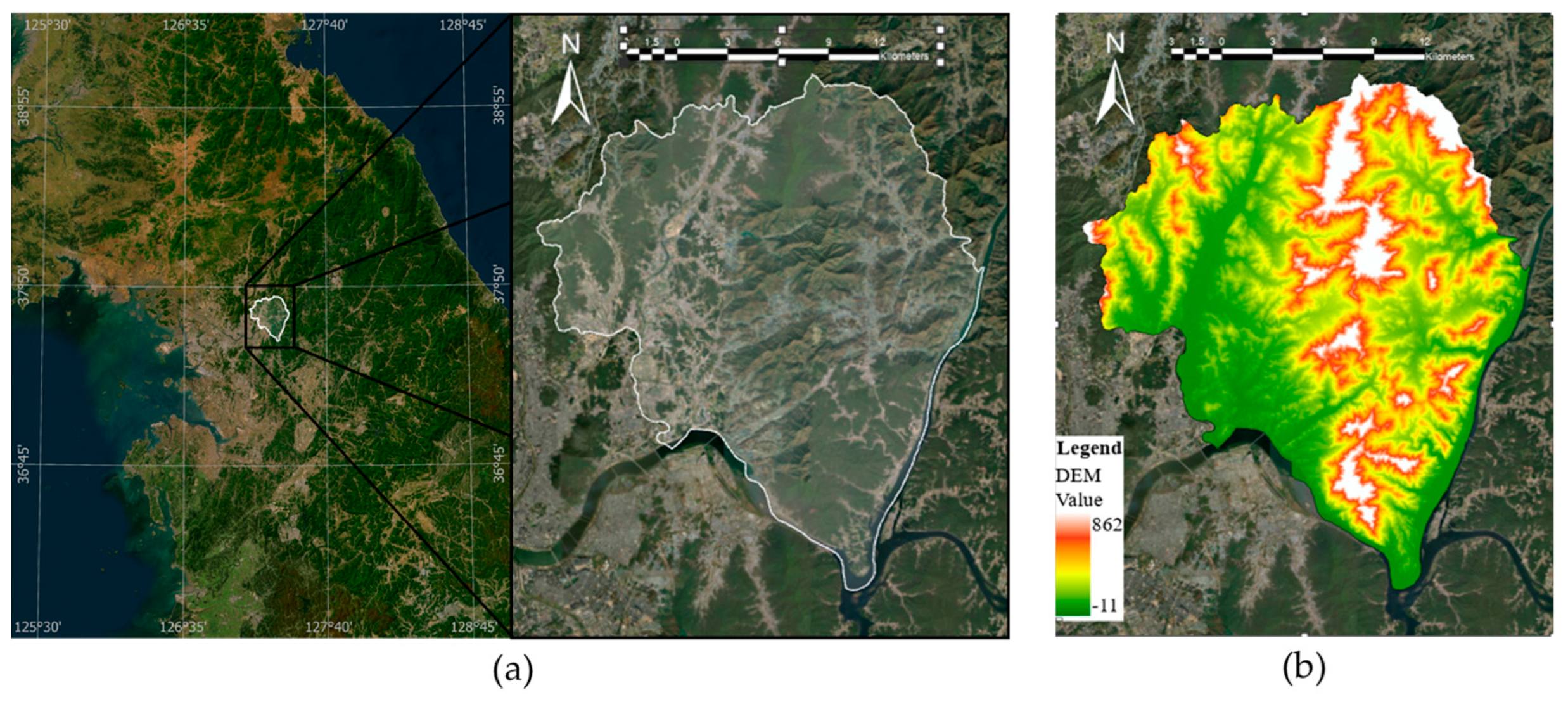
Figure 2.
Acquired cloud-free, multi-temporal Landsat-8/9 scenes over Namyangju during 2023.
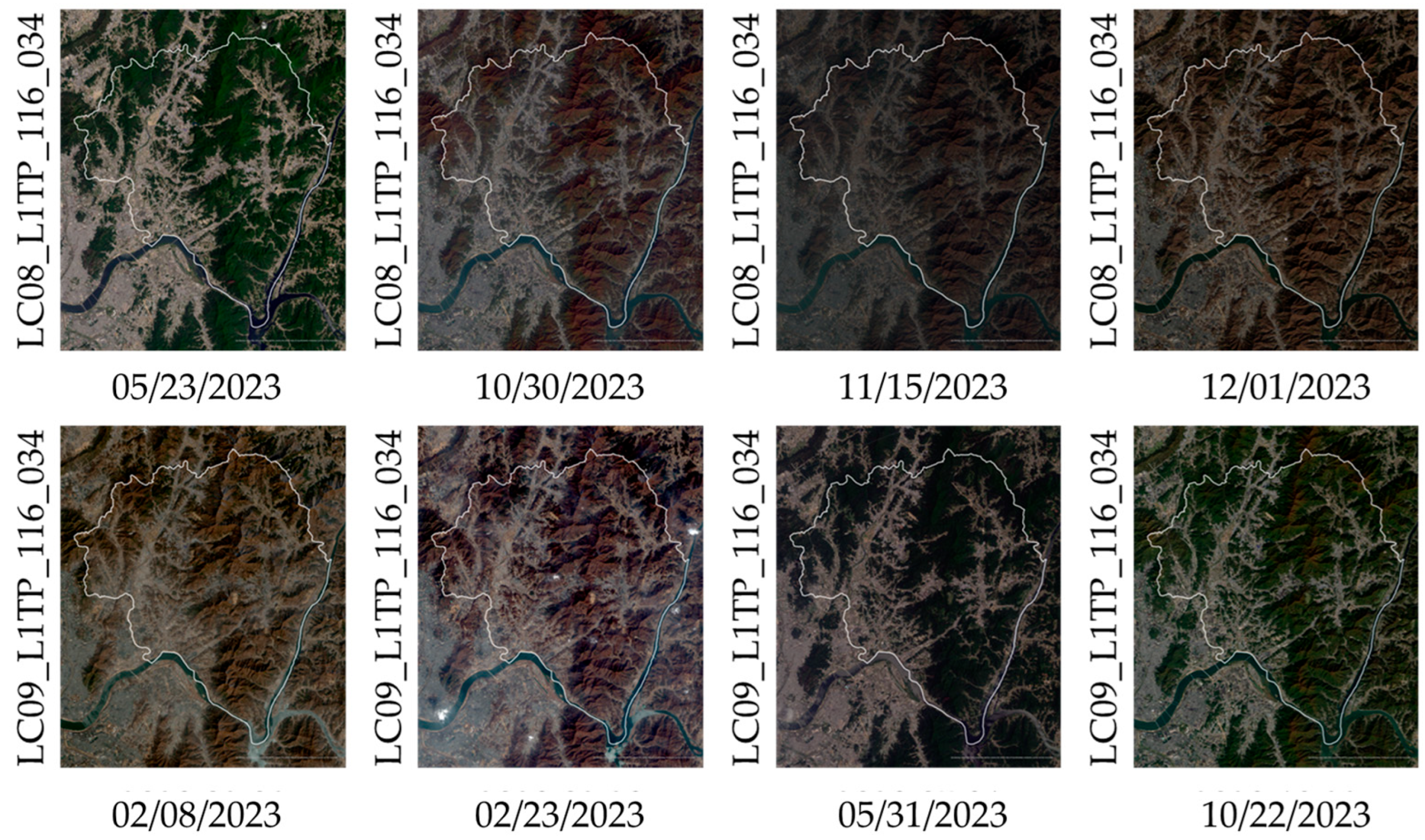
Figure 3.
Flow Chart of this study.
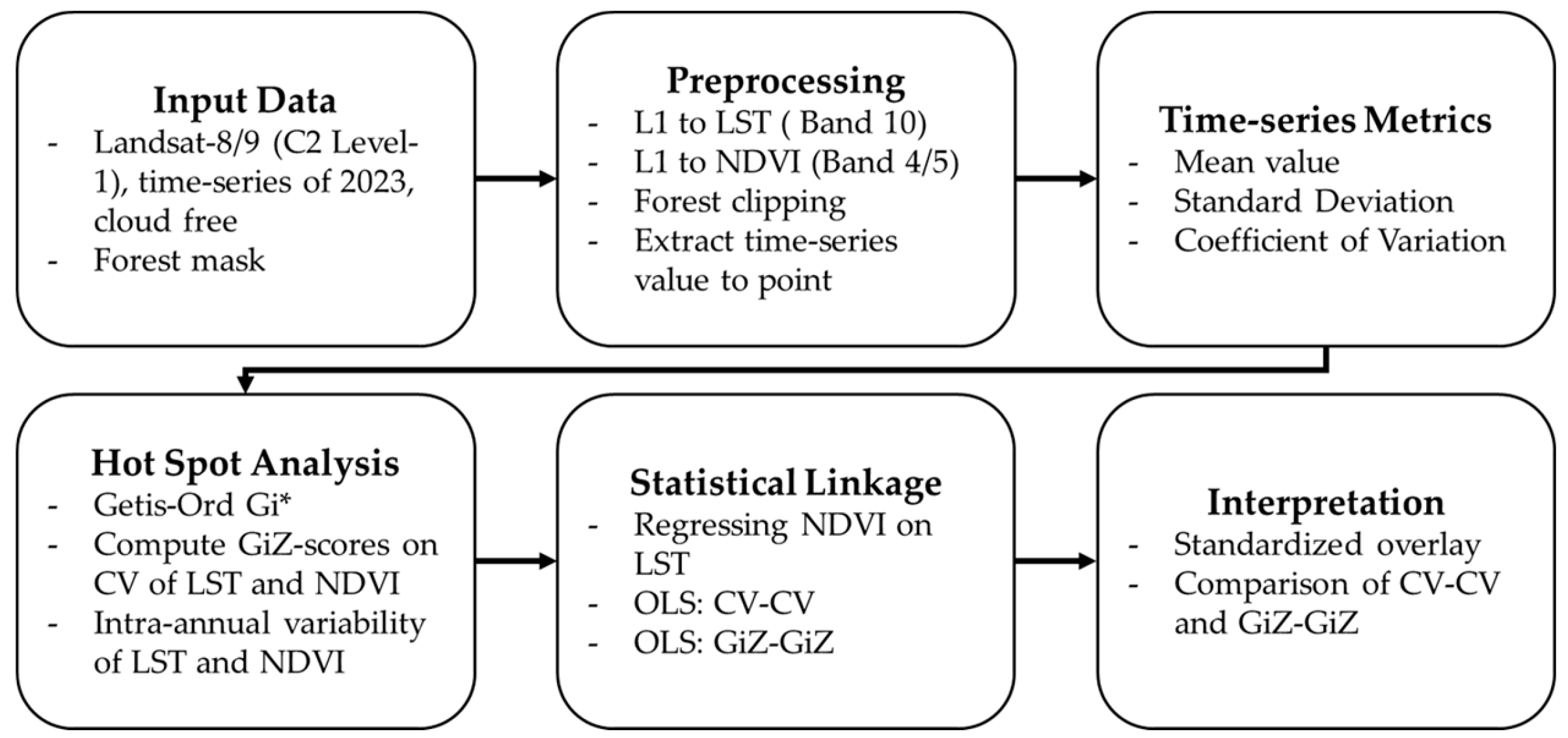
Figure 4.
Getis–Ord Gi* hotspot maps of the annual coefficients of variation (CV) and Altitude of Namyangju: (a) LST; (b) NDVI; (c) Management-priority sites.
Figure 4.
Getis–Ord Gi* hotspot maps of the annual coefficients of variation (CV) and Altitude of Namyangju: (a) LST; (b) NDVI; (c) Management-priority sites.
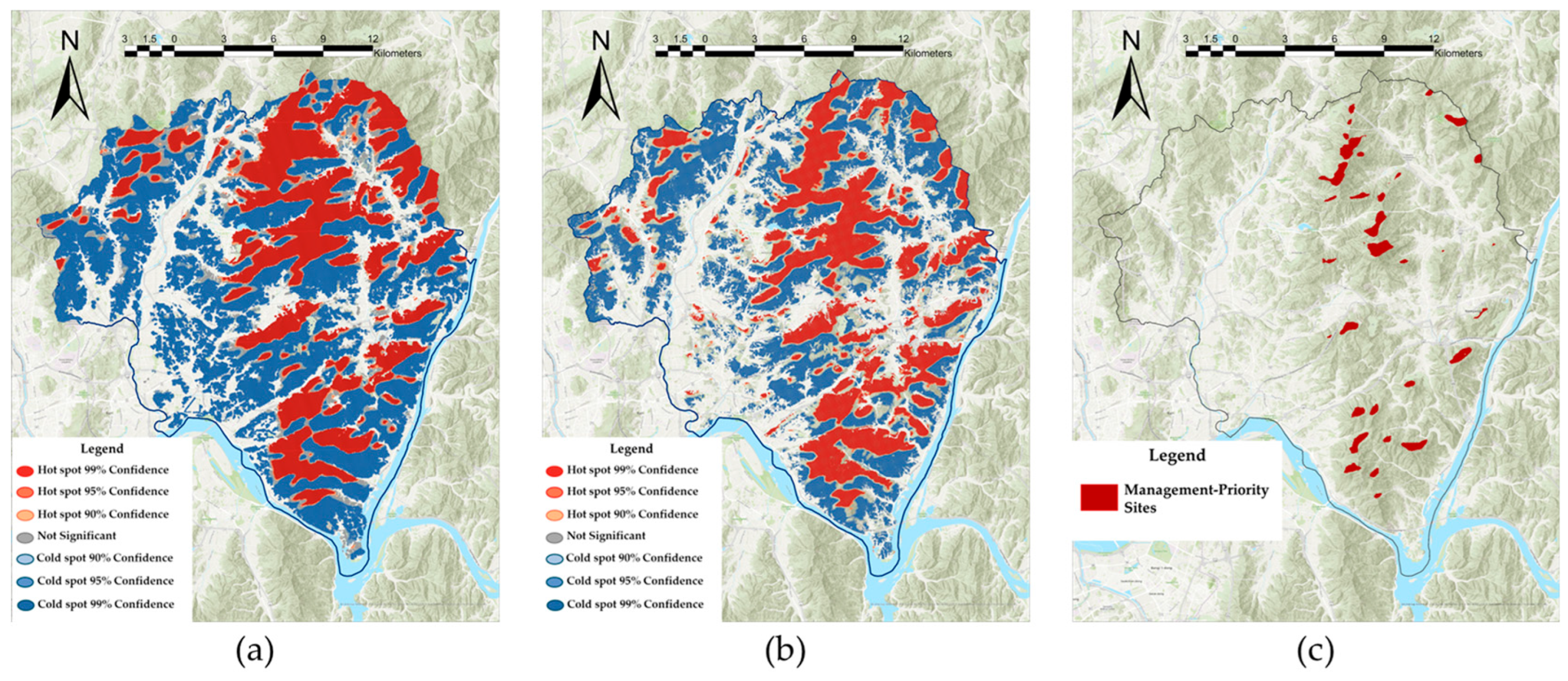
Figure 5.
Comparison of LST–NDVI relationships: (a) CV vs CV; (b) GiZ vs GiZ; (c) Standardized graph.
Figure 5.
Comparison of LST–NDVI relationships: (a) CV vs CV; (b) GiZ vs GiZ; (c) Standardized graph.
Disclaimer/Publisher’s Note: The statements, opinions and data contained in all publications are solely those of the individual author(s) and contributor(s) and not of MDPI and/or the editor(s). MDPI and/or the editor(s) disclaim responsibility for any injury to people or property resulting from any ideas, methods, instructions or products referred to in the content. |
© 2025 by the authors. Licensee MDPI, Basel, Switzerland. This article is an open access article distributed under the terms and conditions of the Creative Commons Attribution (CC BY) license (http://creativecommons.org/licenses/by/4.0/).
Copyright: This open access article is published under a Creative Commons CC BY 4.0 license, which permit the free download, distribution, and reuse, provided that the author and preprint are cited in any reuse.


