
Submitted:
19 March 2024
Posted:
19 March 2024
You are already at the latest version
Abstract
Remote sensing technologies are critical for analyzing the escalating impacts of global climate change and increasing urbanization, providing vital insights into land surface temperature (LST), land use and cover (LULC) changes, and the identification of urban heat island (UHI) and surface urban heat island (SUHI) phenomena. This research focuses on the nexus between LULC alterations and variations in LST and air temperature (Tair), with a specific emphasis on the intensified SUHI effect in Kharkiv, Ukraine. Employing an integrated approach, the study analyzes time-series data from Landsat and MODIS satellites, alongside Tair climate records, utilizing machine learning techniques and linear regression analysis. Key findings indicate a statistically significant upward trend in Tair and LST during summer months from 1984 to 2023, with a notable positive correlation between Tair and LST across both datasets. MODIS data exhibit a stronger correlation R² = 0.879, compared to Landsat R² = 0.663. The application of supervised classification through Random Forest algorithms and vegetation indices on LULC data reveals significant alterations, manifested as a 70.3% increase in urban land, concurrently with a decrement in vegetative cover, especially 15.5% reduction in dense vegetation and a 62.9% decrease in sparse vegetation. Change detection analysis elucidates a 24.6% conversion of sparse vegetation into urban land, underscoring a pronounced trajectory towards urbanization. Temporal and seasonal LST variations across different LULC classes were analyzed using kernel density estimation (KDE) and boxplot analysis. Urban areas and sparse vegetation had the smallest average LST fluctuations, at 2.09°C and 2.16°C, respectively, but recorded the most extreme LST values. Water and dense vegetation classes exhibited slightly larger fluctuations of 2.30°C and 2.24°C, with the bare land class showing the highest fluctuation 2.46°C, but fewer extremes. Quantitative analysis with the application of Kolmogorov-Smirnov tests across various LULC classes substantiated the normality of LST distributions p > 0.05 for both monthly and annual data sets. Conversely, the Shapiro-Wilk test validated the normal distribution hypothesis exclusively for monthly data, indicating deviations from normality in the annual data. Thresholded LST classifies urban and bare lands as warmest classes with 39.51°C, 38.20°C and water by 35.96°C and dense vegetation 35.52°C, sparse vegetation 37.71°C as coldest, a trend consistent annually and monthly. The analysis of SUHI effects demonstrates an increasing trend in UHI intensity, with statistical trends indicating a growth in average SUHI values over time. This comprehensive study underscores the critical role of remote sensing in understanding and addressing the impacts of climate change and urbanization on local and global climates, emphasizing the need for sustainable urban planning and green infrastructure to mitigate UHI effects.
Keywords:
land surface temperature
; land use/land cover
; Landsat
; Modis
; air temperature
; urban heat island
; surface urban heat island
; linear trend
1. Introduction
The prevailing consensus within the scientific community underscores that the observed escalation in global temperatures over the past five decades predominantly transcends natural variability, necessitating an acknowledgment of the profound impact of human activities on climate change. This assertion is supported by a plethora of studies and institutional reports [1,2,3,4,5,6] which collectively highlight the anthropogenic contributions to the warming climate. The escalating effects of global climate change and the rise in urbanization across the globe underscore the importance of enhancing our comprehension of how heat stress affects humans within urban environments [7,8,9,10,11]. Intensive urbanization significantly affects natural ecosystems. The swift pace of urban expansion, which strains essential infrastructure, coupled with the escalation in frequency and severity of weather events linked to global climate change, intensifies the repercussions of environmental hazards [12,13,14,15,16]. Long-term changes in land use/land cover (LULC) [17,18,19,20], stemming from the conversion of natural green spaces and arable lands into impermeable surfaces, are contributing to the formation of urban heat islands (UHI) [21,22,23,24] and the elevation of land surface temperatures (LST) [25,26,27,28,29,30,31,32,33]. Consequently, understanding the intricate dynamics between LST fluctuations and LULC modifications, through the lens of remote sensing technologies, becomes imperative for refining urban planning and management practices [34,35,36,37]. The methodological basis for studying the spatial patterns and temporal dynamics of LST and LULC transformations is the analysis of satellite data, while the source of LST data is thermal infrared range (TIR) [8,9,10,11,12,13,37]. The sensors most frequently utilized for LST are NOAA, Modis [38,39,40,41,42,43], ASTER, AATSR, SLSTR (Sentinel-3 A/B) and Landsat which are freely available [44,45,46,47,48,49,50]. For calculating LST from Landsat satellite imagery, various validated algorithms can be employed as well as diverse methodologies for enhancing the accuracy of LST retrieval and modelling [51,52,53,54,55,56,57]. Approaches to obtaining LST are generally divided into types of the mono window algorithm (MWA), which are based on individual atmospheric parameters such as ambient temperature, humidity, and mean atmospheric temperature [52,54,58,59], the single channel algorithm (SCA) which takes into account the Earth’s emissivity and is conditioned by the water vapour content (w) in the atmosphere [42,51], the split window algorithm (SWA) which uses the different absorptions of two TIR bands, linearizing or no linearizing the radiance transfer equation with respect to the temperature or wavelength [21,24,39,41,51,60,65] and the radiative transfer equation (RTE) which involves the calculation of brightness temperature, proportion of vegetation based on NDVI, and emissivity [106,107]. Many studies are specifically dedicated to comparing the performance of existing methods for obtaining and improving LST data [61,62,63,64,66]. The main statistical approaches and methods commonly used in the study of LST and especially LULC interdependence are supervised and unsupervised techniques [9,20,25,67,68,69,70]; Mann-Kendall statistics [13,71]; principal component analysis end ordinary least squares [72,73]; cellular-automata [21,33,48,74] and most widely used linear and multiple linear regression analyses [9,11,15,28,33,34,35,36,37,38,39,49,57,76]. Particular attention is merited by studies focused on establishing linear and nonlinear dependencies between LST, UHI effects, and various vegetation indices [31,67,77,78,79,80,81,82,83].
Most studies using satellite imagery highlight the complex relationship between changes in LST and LULC, as well as UHI and SUHI phenomena, offering insight into the dynamics of the thermal environment in cities [84,85,86,87,88,89,90,91]. The exploration of UHI effects within various global cities, notably Munich, Germany, Shanghai, China, and Tokyo, Japan, reveals a consistent mitigation impact provided by urban vegetation and water bodies [7,13,32]. A comprehensive analysis demonstrate an increase in LST as areas transition from dense vegetation to sparser vegetation or bare land, with moisture content being a pivotal factor in this proces [8,9,37,80,89,91]. The reduction of urban greenery directly correlates with the expansion of bare land and built-up surfaces, further exacerbating urban temperatures [67,71]. Research into the spatial distribution of LST across various urban and rural settings reveals that populated areas exhibit the highest LST across all seasonal phases, with agricultural lands, vegetation, and water bodies following in descending order of LST intensity [19,24,26,78,81]. This seasonal variability underscores a pronounced dependency on LULC changes, especially during warmer months, with topography and albedo gaining prominence in colder seasons [11,44,93]. Seasonal analyses further delineate the dependency of LST on LULC changes, underscoring the significant influence of vegetation cover and topography on temperature variations [93]. The intricate link between urban development patterns and LST variations has been further elucidated through studies focusing on the configuration of urban spaces [92]. Multitemporal analyses across European cities reveal significant LST disparities between urban centers and their rural counterparts, with SUHI effect exhibiting maximum variation [10,27]. Furthermore, the SUHI effect’s intensity is found to decrease logarithmically or diminish linearly with increasing distance from urban centers [34,35] establishing a clear correlation between LST and biophysical surface parameters. The role of deforestation alongside urbanization in elevating LST in urban areas has been identified, highlighting the necessity to consider population density, construction, and landscape changes [39,73,92]. The examination of local climate zones introduces a nuanced perspective on urban thermal behavior, highlighting the temperature differentials across different urban zones influenced by specific planning and land use patterns [76]. Research underscores the relationship between urban zones, LST, and air temperature, pinpointing vegetation and tall buildings as critical factors influencing LST, while construction density has a lesser impact [92]. Recent advocacies for integrating LST analysis into broader climate change research emphasize the significance of employing additional climatic data and validation methods to refine our understanding of UHI and SUHI effects [15,21,38]. This approach is supported by evidence suggesting that global temperature trends traditionally measured through air temperature data can be effectively mirrored by satellite-derived LST readings, thereby presenting a compelling case for the integration of these data types in urban climate studies [12,40,55,92]. In summary, this body of research collectively underscores the intricate interplay between urban vegetation, LULC and LST changes, and urban planning in modulating urban temperatures.
The primary goal of this study is to elucidate the dynamics between LULC changes, LST, and air temperature (Tair), and how these interactions contribute to the linear increase in LST and the manifestation of SUHI effects in urban settings. The main phenomena addressed in this study are (1) to examine the presence of a global trend in increasing LST and Tair within urban environments; (2) to analyze the spatial and temporal alterations in urban LULC, pinpointing the primary classes undergoing transformation; (3) to explore LST variations and trends in LULC classes, as well as setting thresholds to reveal how land use affects seasonal and annual temperature variations in cities; (4) analyze correlations between SUHI values and environmental factors (LST, Tair, urbanization, and vegetation), and identify temporal trends in SUHI, to understand how significant LULC changes contribute to increases in LST and intensify UHI effects, leading to SUHI phenomena.
2. Materials and Methods
2.1. Study Area
The city of Kharkiv is located in the northeastern part of Ukraine with coordinates latitude: 49° 58’ 50.92” N and longitude: 36° 15’ 9.79” E Figure 1. Kharkiv is recognized as a scientific center of the country. Covering an area of more than 306 km2, it is Ukraine’s second-most populous city, boasting a population of 1,421,125 people, making it the 17th most populous in Europe. The population density stands at 3,875 people per km2. Administratively, it is divided into 9 districts [94,95,96]. Kharkiv is a significant scientific, cultural, industrial, and transport hub, formerly the third-largest industrial center. The topography features the highest point at 202 meters above sea level and the lowest at 94 meters. The city is divided into four lowland and four elevated areas. It has a moderate continental climate with an average annual air temperature of +6.9 °C, the coldest month being January at -6.1 °C, and the warmest July at +20.5 °C. The average annual precipitation is 520 mm, peaking in June and July [96]. Large cities like Kharkiv exhibit unique climatic characteristics, arising from the interplay of natural environmental factors and the impact of human activities. The extensive use of asphalt and other artificial materials significantly alters the city’s underlying surface, contributing to these unique climate conditions. Urban areas are marked by atmospheric pollution, which reduces solar radiation and leads to a suite of climatic modifications: air temperatures in cities are consistently 1-3 °C warmer than those in surrounding rural areas, humidity levels are elevated, winds are diminished, and there is an increase in annual precipitation by 20-30 mm. Moreover, urban environments experience more frequent thunderstorms and exhibit much lower seasonal and daily temperature variations [95,96].
According to the Kharkiv City Development Strategy until 2020 [97], green spaces cover 15.4 kha, providing approximately 15 m2 of green space per capita, and the nature reserve area comprises 467.7 ha. Meanwhile, the city’s industrial enterprises occupy a total area of 4031.4 ha. According to the Kharkiv Sustainable Energy and Climate Action Plan until 2030 [98], the residential buildings sector emerges as the primary source of CO2 emissions, contributing to 60.2% of the total emissions. Furthermore, Kharkiv’s climate change vulnerability assessment underscores grave concerns regarding heat stress and the fragility of urban green spaces, primarily attributed to the city’s heavy, energy-intensive industries. These sectors augment urban atmospheric heat, escalating heat stress risks. Compounding this issue is the pronounced scarcity of green spaces in the city’s northeastern, eastern, and southeastern districts, areas predominantly occupied by industrial zones [97,98]. However, since February 2022, the escalation of military actions by the Russian Federation against Ukraine has profoundly impacted Kharkiv’s economic, environmental, and social structures, exacerbating the situation. The conflict has not only led to a stark demographic decline but also inflicted considerable damage on the city’s industrial base. In urban ecological terms, such disturbances induce marked land cover variability [99]. Considering the information provided above, the results of our study will primarily serve as a tool for assessing the thermal conditional of the city environmental through the lens of both intense urbanization and adaptations to global climate changes using remote sensing. This is particularly relevant during military actions, as ground-based methods are impossible.
2.2. Data
This study utilized Landsat imagery, accessed via the Google Earth Engine (GEE) cloud platform, spanning a period of 40 years from 1984 to 2023. The primary objective was to analyze the changes in LULC and LST. The dataset comprises atmospherically corrected surface reflectance and land surface temperature values. These were derived from data produced by the Landsat 5, 8, and 9 Operational Land Imager/Thermal Infrared Sensor (OLI/TIRS) systems. The imagery encompasses four (Landsat 5) or five (Landsat 8-9) visible and near-infrared (VNIR) bands, along with two short-wave infrared (SWIR) bands. These bands have been processed to yield orthorectified surface reflectance. Additionally, there is a thermal infrared band (specific to Landsat 8-9) processed to provide orthorectified surface temperature data. The dataset also includes intermediate bands pivotal in the computation of surface temperature (ST) products, complemented by quality assessment (QA) bands [100,101,102]. The selection interval for the imagery was strategically determined to mitigate the impact of cloudiness and snow cover, which significantly influence the accuracy of LST measurements. The presence of even minimal cloud cover can notably distort LST data acquisition. Therefore, imagery selection was confined to the months of April through September, with a stipulation for cloud cover to be less than 10%, ensuring weather clarity. This selection criterion, however, meant that imagery for certain months or years was not always available.
In addition to the Landsat data, LST data were obtained from the MOD11A1 V6.1 product from 2000 to 2022. This product provides daily LST and emissivity values on a 1200 x 1200 kilometer grid, derived from the MOD11_L2 swath product. The MOD11A1 V6.1 product includes both day-time and night-time surface temperature bands along with their quality indicator layers. It also features MODIS bands 31 and 32, and six observation layers, further enriching the dataset. LST pixel values are generated using the split-window algorithm with clear-sky conditions and are averaged in areas with overlapping pixels with overlapping areas of weight [43].
In the context of this study, the utilization of average monthly temperature data, sourced from the Climatic Research Unit (CRU) Time-series (TS) Version 4.07, enhances the precision in examining LST changes. The CRU TS 4.07, a product of the meticulous research conducted by the Climatic Research Unit at the University of East Anglia and financed by the UK National Center for Atmospheric Science (NCAS), a NERC collaborative centre, offers month-by-month climatic variations spanning from 1901 to 2022. These data are presented on high-resolution grids of 0.5 x 0.5 degrees, enabling a detailed and nuanced understanding of climatic patterns. The variables encompassed within the CRU TS4.05 dataset are comprehensive and diverse, including cloud cover, diurnal temperature range, frost day frequency, wet day frequency, potential evapotranspiration, precipitation, daily mean temperature, monthly average daily maximum and minimum temperature, and vapor pressure. The granularity of this dataset, with its high-resolution grid format, allows for a detailed spatial analysis of climatic variables, offering insights that are critical in understanding the nuanced variations in land surface temperatures [103].
In Table 1 summarizes the datasets used in this study. The full Landsat datasets is presented in Supplementary: Table S1.
Upon meticulous analysis of the data collated for this study, it is pertinent to acknowledge the extensive temporal coverage spanning from over a near four-decade timeframe. The protracted duration of this dataset is paramount in elucidating long-term trends and fluctuations in LST and land cover modifications. Moreover, a predominant portion of the imagery exhibits a minimal cloud cover percentage, indicative of the high caliber of the dataset for analytical purposes. Such clarity is of critical importance in the precise determination of LST. The reduced cloud interference in these images assures a heightened degree of reliability and accuracy in the temperature readings. In addition, the dataset portrays a spectrum of air temperature and precipitation measurements, both of which are pivotal in influencing LST. A notable aspect of these observations is the predominance of minimal to zero precipitation readings. This pattern suggests that the recorded LST values are less prone to alteration by immediate moist conditions, thereby more accurately reflecting the actual land surface conditions as opposed to ephemeral meteorological variations.
2.3. Methods
2.3.1. Retrieval of LST Using RTE
The RTE is one of the most used methods of LST retrieval which involves the calculation of brightness temperature, proportion of vegetation based on NDVI, and emissivity (E), and was calculated on the GEE platform [104,106,107]. In the first step, the brightness temperature was obtained from the Landsat surface reflectance (SR) collection using Equation (1).
where, Tb - represents the brightness temperature, ST - is the pixel value from thermal band 6 (ST_B6) for Landsat 5 and band 10 (ST_B.*) for Landsat 8/9. This formula converts the digital pixel values of band 6 (band 10) into brightness temperature. The factor 0.00341802 and the constant 149.0 are calibration parameters that transform the digital values into temperature in Kelvin or Celsius (depending on the original settings of the sensor).
The next step is calculating the NDVImin and NDVImax values. NDVI is a widely utilized metric for estimating the proportion of vegetation (pv) [105]. Pv is calculated using the following Equation (2).
where NDVImin and NDVImax are the NDVI values for pixels without vegetation and pixels with vegetation. Based on previous studies [51,54,58], these thresholds are NDVImin is 0.2 for bare land and NDVImax is 0.86 for vegetation area.
The calculation of emissivity (E) using the pv can be represented using Equation (3).
where 0.004 coefficient represents the E variation due to vegetation, and 0.986 represents the base E for other surfaces. E values near 1.0 are typical for natural surfaces like bare land and vegetation, while lower values are often associated with water bodies or urban areas [54,55,104]. This is a common approach in remote sensing to estimate surface emissivity using vegetation information.
Calculating LST and representing it in Celsius using Equation (4).
where Tb is the brightness temperature, obtained from the thermal band of the satellite imagery, E is the emissivity (3), the constants 0.00115 and 1.438 are part of the Planck’s function related constants for converting brightness temperature to LST. The subtraction of 273.15 at the end is to convert the temperature from Kelvin to Celsius [62,106,107].
2.3.2. LULC Classification and Change Detection
LULC classification, Landsat imagery was processed using the Random Forest (RF) technique within GEE platform [108,109,110]. The initial phase of the classification procedure necessitated the preparation of training samples. In our study, these samples were methodically developed based on distinct landscape elements of the study area. The creation of training samples involved the meticulous digitization of image pixels that accurately represent each class, ensuring uniformity to minimize classification errors. Adhering to established guidelines, a minimum of 50 training samples per class was generated, culminating in a total of 1045 training samples. The allocation of these samples was proportionate to the prevalence of each LULC class within the study area, with a deliberate and even distribution across the territory of Kharkiv city. For the implementation of the RF algorithm, the selection of the number of decision trees is a critical input parameter [110]. In this instance, 100 trees were utilized, as per standard recommendations. After the classification is completed, it is necessary to evaluate its accuracy. To do this, we created additional samples: 376 points, evenly distributed over the image Table 2.
In the classification process, our methodology extended beyond the mere application of spectral bands [111]. It included a comprehensive analysis of multiple vegetative indices, including NDVI, NDBSI (Normalized Difference Bare Soil Index), BAEI (Built-up Area Extraction Index), NDWI (Normalized Difference Water Index), NDBI (Normalized Difference Built-up Index), BRBA (Band Ratio for Built-up Area), NBAI (Normalized Built up Area Index), IBI (Index-Based Built-up Index), NBI (New Built-up Index), and UI (Urban Index) to enhance the differentiation of spectral similarities among classes [112,113,114,115,116]. Each of these indices contributes uniquely to the precise classification of the land cover, by leveraging specific spectral characteristics inherent to each class.
To evaluate the accuracy of the resultant LULC maps, a comprehensive accuracy assessment was conducted. This involved the compilation of a confusion matrix, from which key descriptive statistics were calculated to assess classification efficacy. These statistics included overall accuracy (OA), producer’s accuracy (PA), user’s accuracy (UA), and the Kappa coefficient (Kappa), providing a robust measure of the classification’s reliability and precision [117].
To rigorously assess the temporal variations in the spatial extent of distinct classes between 1984 and 2023, we employed the advanced change detection algorithm specific to categorical data within the ArcGIS PRO framework. This methodology enables a precise and comprehensive analysis of alterations in LULC categories over the specified period [115].
When classifying the Landsat 5 imagery from 1984 to 1990, significant challenges arose in distinguishing between urbanized areas and bare land due to their similar spectral signatures. To address this issue, topographic lists of the map of Kharkiv, specifically list M-37-073 and list M-37-061 at a scale of 1:100,000, were utilized [124]. These maps, created by the General Staff of the Soviet Union, depict Kharkiv’s territory during 1986-1990. Subsequently, these map lists were merged to represent the territory’s entirety. Then georeferenced coordinates and cropping were performed using the area shapefile in ArcGIS PRO. The final map was incorporated into our project on the GEE.
2.3.3. Trend Analysis Methods and Statistical Distribution
To determine the trend of increase or decrease in Tair, LST, linear regression analysis was used, with the determination of the slope, coefficient of determination (R2), level of significance (p-value) and Mann-Kendall test (τ), p (τ) [9,11,30,31,32,33,118,119]. For comparison of Tair, LST by Landsat and Modis was also used root mean square error (RMSE) [72,73]. For correlation analysis between SUHI mean and Tair, LST, urban area and vegetation area we used Pearson’s (rx,y), Spearman’s (ρ) coefficient of correlation and standard error (SE) [117]. The relationship between different LULC classes and LST was established by using Kernel Density Estimation (KDE) [120]. KDE is used to estimate the probability density function of LST data for different LULC classes. By applying KDE was visualized the distribution of LST values within each LULC class, identify patterns, and assess the variability of LST across different land covers. From this distribution, was extracted several important parameters for each class. The peak of the KDE plot represents the most common values or the mode of the distribution for a particular class. The width of the KDE curve gives an idea about the variance or spread (Sp) of the data. The asymmetry of the KDE plot is shown about the skewness (Sk) of the data distribution. Multiple peaks in the KDE plot suggest the presence of multiple sub-groups or a multi-modal (MM) distribution within the class. Boxplot parameters such as median (Med) a central tendency measure of data. Interquartile Range (IQR) the box length shows the IQR, which is the range between the 25th percentile (Q1) and 75th percentile (Q3). It indicates where the middle 50% of the data lies. Dots outside the ‘whiskers’ of the boxplot represent outliers (Out). These are data points that are significantly higher or lower than the rest of the data and could indicate anomalies [121].
2.3.4. Statistical Distribution of UHI and SUHI Value
To determine UHI index for each point on the surface Equation (5) was used.
where LST is the LST at each point on the surface, measured in °C, µLST - is the mean LST for the entire area, measured in °C, σLST - is the standard deviation of the LST for the entire area [16,32,84,85].
The calculation of pixel-wise SUHI can be represented mathematically by Equation (6).
is the value for the pixel located at the i row and j column of the urban area,
is the LST at the pixel located at the i row and j column of the urban area,
is the average LST across all pixels classified as vegetation (dense vegetation, sparse vegetation) [10,27,36,46,87,91]. The urban mask is applied to the resampled LST data to extract the temperatures for urban areas, while the vegetation mask is applied to do the same for vegetation areas. Then the average vegetation temperature is subtracted from the urban temperature for each corresponding pixel, resulting in the SUHI map.
3. Results
Since the overall goal of this study was to elucidate the dynamics between changes in LULC, LST and air temperature (Tair), and how these interactions contribute to the linear growth of LST and the manifestation of SUHI effects in urban environments, our results are presented in a stepwise manner in the sections.
3.1. Establishing a Global Trend of Increasing Tair and LST
3.1.1. Analysis of Air Temperatures Tair
While investigating climatological dynamics, we utilized the CRU TS, to construct a heatmap representing the temporal progression of Tair and monthly average temperatures are shown in Figure 2.
This visualization encapsulates the thermal variances within the city of Kharkiv, offering insights into the climatic trends over an extensive period. This heatmap not only identifies the extremities in temperature experienced over the years but also serves as a crucial tool in discerning potential patterns and anomalies in the climate data. Such a detailed depiction of temperature shifts is pivotal for advancing our understanding of the regional climate behavior in Kharkiv across the span of multiple decades. The coldest month recorded was December 1996, plunging to -10.7 °C, an outlier in the dataset indicative of a significant climatic anomaly. Conversely, the warmest month appears to be July 2006, soaring to 24.9 °C, which marks it as a notable peak in the recorded temperature spectrum. A consistent pattern of warmer temperatures is evident during the mid-year months, particularly in the past decade, suggesting a potential shift towards higher summer temperatures. The data underscores the necessity for scrutinizing the extremities within the climatic sequence to understand the breadth and implications of temperature variability over the span of recent decades.
Upon analyzing the created climate data table, the results reveal notable seasonal patterns and statistically significant trends in Tair and are shown in Table 3. Particularly, the months of June, July, August, and November exhibit substantial and statistically significant positive slopes in Tair trends (0.059, 0.059, 0.074, and 0.082, respectively), as indicated by their low p-values (0.003, 0.001, 0, and 0.003, respectively). This is further substantiated by the high τ values for these months, especially August (0.493), which, coupled with their low p (τ), suggests a robust upward trend in Tair (Table 3).
Figure 3.
Decadal analysis of global Tair trends 1981-2022 (CRU TS).
These findings underscore the criticality of these months in the context of rising Tair. The analysis of the annual trend Tair elevation yielded statistically significant outcomes, with R2 0.414 and τ = 0.487, respectively. This relationship is illustrated in the Table 3.
3.1.2. Analysis of LST Based on Landsat
In the subsequent phase of the research, we constructed LST maps encompassing all available temporal data points (Figure 4 and Figure 5). This analysis was aimed at meticulously examining the trajectory of changes specifically pertaining to the rise in surface temperatures. The methodology employed in developing these LST maps facilitates a focused analysis on the patterns and magnitude of surface warming, thereby enabling a nuanced understanding of the temporal dynamics of surface temperature elevations. Such an approach is pivotal in discerning the subtleties of climate change impacts, particularly in the context of surface temperature variations over the studied period. Since the climate data showed a sufficient trend showing an increase in air temperature in months such as June, July, August and November (Table 3), further analysis was focused on these months.
Trends in July LST. Due to significant cloud cover during the observation period, our July image collection comprises only 17 observations. Analysis of July trends from 1984 to 2023 reveals that areas with the highest LST are predominantly located in the city center, extending to the northeast and southeast, as depicted in Figure 4. Annual analysis indicates a notable thermal anomaly in 2016, where the average LST peaked at 45 °C. Similarly, high LST values were recorded in 2018 and 2020, reaching 41.4 °C, in stark contrast to the 1980s and 1990s, when LST values were observed at 32.8 °C and 34.9 °C, respectively. Trends in August LST. Analysis of LST in August, based on 20 observations, distinctly highlights a warming trend. It is particularly noteworthy that recent years have exhibited a gradual increase in LST. For instance, in 1986, 1992, and 1996, LSTs were recorded at 35.9 °C, 32.5 °C, and 31 °C, respectively. In contrast, the period from 2017 to 2023 experienced a higher average LST exceeding 40 °C. This trend suggests a continuous rise in mean LST for August across the years. Elevated values in certain years signify extreme LST occurrences. Trends in June LST. The June image dataset comprises 14 observations, yet it similarly reveals a general trend of increasing LST over the years. For instance, the average LST in June was 37.3 °C in 1986, which rose to 40.7 °C by 2020. The peak average LST reached 44.5 °C in 2019, denoting exceptionally high temperatures in recent years Figure 5. Although variability in LST is observed throughout the studied period, the overall trend indicates a continuous increase during the summer months.
The interpretation of statistical results as for April (Month 4) and May (Month 5) exhibit a decreasing trend but not statistically significant. In June (Month 6) and September (Month 9) display a slight increasing trend (slope: 0.052 and 0.070), but not statistically significant (p-value: 0.547 and 0.531). In July (Month 7) indicates a moderate increasing trend (slope: 0.0910) and nearing statistical significance (p-value: 0.131). In August (Month 8) shows a more pronounced increasing trend (slope: 0.133), which is statistically significant (p-value: 0.041). The number of observations for each month ranging from 11 to 20 impacts the reliability and statistical significance of the trend analysis (Table 4). More observations, as seen in August, tend to give more statistically significant results. Fewer observations can lead to weaker statistical support for any identified trends. However, it’s also evident that even with a greater number of observations, the trend might not always be significant if the natural variability of the data is high, as seen in April and May. This suggests that while the quantity of data is important, the quality and inherent variability of the data are also crucial in determining the significance of trends.
3.1.3. Analysis of LST Based on Modis
Analysis of monthly mean LST trends using MODIS provides an in-depth view of April to September mean LST trends for the period 2000 to 2022 Figure 6.
The linear trend analysis reveals varied trends across the months. In April (Month 4) shows a slight increasing trend (slope: 0.045) but not statistically significant (p-value: 0.544). While in May (Month 5) indicates a negligible decreasing trend (slope: -0.019), with no statistical significance (p-value: 0.843). The significance of the trend is monitored in June (Month 6) and September (Month 9) presents a notable increasing trend (slope: 0.202 and 0.131), which is statistically significant (p-value: 0.023 and 0.116). Intriguing is the fact that July (Month 7) and August (Month 8) show a moderate increasing trend but not statistically significant (Table 5).
The analysis indicates a general trend of increasing LST in Kharkiv during the summer months from 1984 to 2023. Notably, recent years have experienced higher LST as seen in 2016 and 2019. This trend could be attributed to factors such as UHI effect, climatic changes, factors such as urbanization, land use changes, and environmental factors could also be contributing to these observed changes in LST patterns. This analysis suggests a need to consider broader climatic trends and local environmental changes to fully understand these LST patterns.
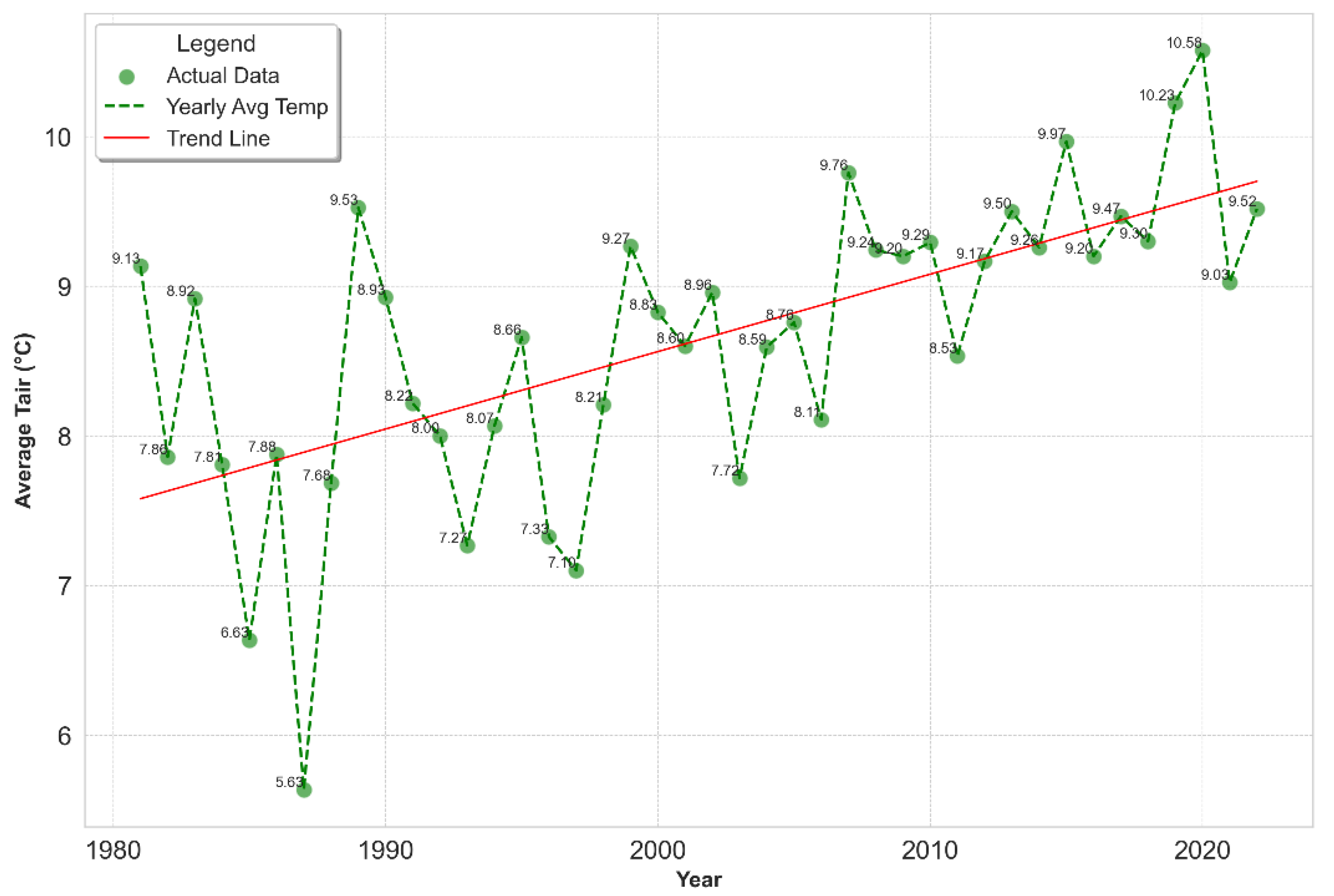
3.1.4. Comparison of Tair and LST by Landsat and Modis
Comparing Tair with LST from Landsat and MODIS satellites helps to understand the UHI effect in cities such as Kharkiv, revealing temperature fluctuations caused by urban infrastructure. On the one hand, high-resolution Landsat data is critical for pinpointing hot spots in urban areas. While Tair and LST coupling analysis helps in climate change research by tracking how urbanization affects the local microclimate at different scales of observation, from local (30 m with Landsat) to regional (1 km with MODIS) Figure 7.
In summary, both datasets show a statistically significant (p < 0.05) positive correlation between Tair and LST, with MODIS data showing a slightly stronger relationship (R2 = 0.879) than Landsat data (R2 = 0.663). The MODIS data also has a lower RMSE = 1.476, indicating a more accurate model in terms of prediction error (Figure 7, Table 6).
The statistical analysis conclusively demonstrates a discernible pattern of rising temperatures within Kharkiv’s urban environment. This trend is not solely attributable to urbanization and its associated modifications to land surfaces, which is reflected in the increasing LST. It is also a manifestation of the broader phenomenon of global warming, as indicated by the significant correlation between Tair and LST. These findings underscore the intricate interplay between localized urban development and overarching climatic shifts, emphasizing the dual impact on the thermal dynamics of the region.
3.2. LULC Transformation
Temporal classification analysis of satellite-derived land cover datasets from 1984 to 2023 has elucidated substantial alterations in various land class areas (Figure 8). Subsequent to the implementation of image classification techniques, confusion matrices were generated, providing a detailed representation of classification accuracy on an annual basis. Consequently, it was observed that the overall accuracy in water classification, denoted by UA and PA, attained a remarkable 99%. In contrast, the dense vegetation class exhibited a UA of 90% and a PA of 86%. The urban area class displayed a high level of accuracy, with a UA of 92% and PA of 97%, an achievement likely attributable to the integration of additional spectral indices within the classifier, enhancing the identification of artificial structures. The bare land class demonstrated a UA of 87% and a PA of 84%. Notably, the sparse vegetation class exhibited the lowest accuracy rates, with a UA of 78% and a PA of 77% Table 7. It is important to highlight that the overall accuracy of these classifications exhibited a range between 80% and 95%
Analysis of the dynamics of changes in the area showed that the water area increased by about 65%, while dense vegetation decreased by 15.5%. Urban areas experienced the largest changes and increased by about 70.3%. Bare land, which is usually the least in urban environments, showed an increase of about 61%. While the sparse vegetation class decreased by 62.9% (Figure 8). These changes reflect a significant shift in land use patterns in this urban area, emphasizing the expansion of cities and the corresponding decrease in natural vegetation cover.
The largest proportion about 24.6% of the total area is observed in the transition from sparse vegetation to urban land. This indicates a significant urbanization trend. Dense vegetation to urban and sparse vegetation: these transitions are also significant, with about 5.1% and 3.7% of the total area, respectively, indicating a reduction in dense vegetation areas. Various smaller transitions are noted, such as from water to urban or bare land to urban, but these represent smaller fractions of the total area. A notable proportion 51.8% of the area remained unchanged, indicating stability in certain land cover types. As we can see on the constructed map Figure 9, this area is mainly under the central urban area.
3.3. LST Thresholds for Various LULC Classes across the Year and Different Seasons
KDE and its metrics were used to analyze the temperature conditions of each LULC class based on July LST by 1984 to 2023 years are presented in Supplementary: Table S2. The average LST for urban areas shows fluctuations over the observed years, with an overall increase from 1984 - 39.39 °C to a peak in 2020 - 42.46 °C, followed by a slight decrease in 2023 by 39.30 °C. This fluctuation is indicative of the variability of urban temperatures, possibly influenced by urban development, land use change, and climate variability. However, it may also be a result of the shutdown of industry and the population decline due to the war (from 2022). The number of emissions representing extreme LST values has generally increased over time, indicating more frequent extreme temperatures in cities. This may be due to an increase in the UHI effect. The skewness of the LST distribution in cities shows little variation over time, with mostly positive values indicating a right-handed distribution, indicating more frequent extreme high temperatures (Figure 10a–d and Table 8). KDE histograms and boxplot graphs of LST and LULC classes for July other years are presented in Supplementary: Figure S1–S6.
The LST of dense vegetation shows fluctuations over the years with a notable decrease in 2023 to 34.65 °C. However, in 2020, 2028, and 2014, there was a noticeable increase at 38 °C. These changes may reflect changes in density as well as broader climatic conditions. There is a general upward trend in emissions, with peaks in certain years as 1996 and 2011, which may indicate more extreme temperature conditions. The IQR and spread fluctuate over time, indicating changes in LST distribution. In 2006 and 2023, the IQR values were higher (6.90 and 6.69, respectively), indicating increased LST variability in these years. The skewness index indicates a distribution towards higher temperatures over the years. Urban areas and sparse vegetation had the smallest average LST fluctuations, at 2.09 °C and 2.16 °C, respectively, but recorded the most extreme LST values. Water and dense vegetation classes exhibited slightly larger fluctuations of 2.30 °C and 2.24 °C, with the bare land class showing the highest fluctuation 2.46 °C, but fewer extremes, and a noticeable distribution towards higher temperatures, but it is worth noting that there are not many extreme values are observed (Table 8, Figure 10).
The presented graph Figure 11 and Figure 12 illustrate the mean LST distributions for various LULC classes across April to September and from 1996 to 2023, using Gaussian KDE. Solid and dashed lines depict empirical and theoretical distributions, respectively. The theoretical normal distribution is estimated from the mean LST and standard deviation of the collected data. Analyzing Figure 11 where the maximum LSTs for both distributions are marked, the area difference under the curves (deviations are highlighted, with “Empirical Excess” in class colours and “Theoretical Excess” in grey) measures that water (0.010) and bare land (0.002) have the smallest differences, suggesting that their empirical distributions are quite close to the normal distribution in terms of their overall “mass”. Dense vegetation (0.017), urban areas (0.021), and sparse vegetation (0.016) show a larger difference, indicating a more significant deviation from the normal distribution. The varying area difference values indicate that while the RMSE=0.010 between the empirical and theoretical distributions is the same, the distributions themselves have different shapes and “mass”. This due to characteristics unique to each class, such as the distribution of values, the impact of outlier values (Out), the skewness (Sk) of the distribution, or the presence of multiple peaks (MM) and this corroborate with values in Table 8.
In turn, analysing Figure 12 the monthly RMSE analysis reveals that June and July exhibit the highest deviations from the theoretical distribution across all classes, with RMSE values of 0.032 and 0.045, respectively. Conversely, April and May, with an RMSE of 0.021, along with September at 0.024, display moderate deviations. August presents the lowest mean RMSE at 0.018, signifying the closest alignment between distributions. Regarding area difference, April records the highest mean at 0.152, with July following at 0.116, highlighting significant discrepancies across all classes. The smallest mean area differences are observed in June (0.099), May and August (both approximately 0.10), suggesting the nearest overall conformity to theoretical distribution normality.
Shapiro-Wilk (S-W) and Kolmogorov-Smirnov (K-S) tests assess normality, revealing discrepancies. S-W indicates non-normality (p < 0.05), whereas K-S suggests normality (p > 0.05), highlighting the complexity of interpreting statistical normality in Figure 11. While the evaluation of LST distribution normality across each LULC class, segmented monthly, substantiated the data’s normality through both S-W and K-S tests (p > 0.05), thereby affirming statistical significance and shown in Figure 12.
To calculate the thresholds for each class was used the combination of median, IQR, min LST, max LST, and skewness (Table 9).
Urban areas and bare land are the hottest LULC classes, with the highest median LSTs approximately 39.51 °C and 38.20 °C and significant variability, particularly for bare land. Water bodies are the coolest with the median LST around 35.96 °C and moderate variability. Vegetation as a dense - 35.52 °C and sparse - 37.71 °C, show a cooling effect compared to non-vegetated surfaces, with dense vegetation providing more cooling than sparse. The standard deviation across all classes indicates the degree of variability within each LULC class, with urban areas showing the least variability, suggesting a more homogeneous temperature distribution (Table 9).
LST from April to September from 1996 to 2023 was used to determine the seasonal threshold classes. The statistical analysis was performed using the data presented in Supplementary: Table S3, and shown in Table 10.
Analyzing the data in Table 10, it is clear that water and dense vegetation have the lowest average LST values during all months, starting at 20.97 °C in April and reaching a maximum of 36.79 °C in June, and then decreasing again to 34.49 °C in August and continuing through September. This demonstrates the ability of the water to withstand low temperatures and the dense vegetation to have a cooling effect through transpiration. Urban areas show the highest average LST during these months, starting at 22 °C in April and reaching a peak of 40.69 °C in July. This indicates an UHI effect, where urban materials absorb and radiate solar energy more than natural landscapes. The bare ground also shows high average LST with a peak of 40.54 °C in June. This reflects the lack of vegetation cover and the high heat capacity of bare soil. Mean LST in sparse vegetation are lower, from 21.82 °C in April to 38.75 °C in June, than in urban areas and bare land, but higher than in dense vegetation and near water bodies, indicating a moderate cooling effect due to less dense vegetation. Lower thresholds (LT) increase from April to June and decrease towards September for all classes, indicating the onset of warmer conditions in June and a gradual cooling towards September. Upper thresholds (UT) follow a similar pattern, peaking in June and July, which represents the height of summer LST across all LULC classes.
3.4. LULC Transformation Impacts SUHI Dynamics
Using LULC and LST data, spatial maps of SUHI effects for 1984-2023 were constructed. These maps demonstrate a striking increase in the UHI effect of Kharkiv Figure 13a,b. Some of the July maps are presented in Supplementary: Figure S7.
The correlation analysis between SUHI mean and LST and Tair, as well as the proportions of urbanized and vegetated areas, revealed a moderately strong positive relationship between SUHI mean and urbanized areas in both July (0.55) and August (0.53). Conversely, there is a moderately strong negative correlation between SUHI_mean and vegetation area (-0.52 in July and -0.56 in August). The p-values associated with all three types of correlation indicate that this relationship is statistically significant (p < 0.05). However, LST and Tair in July showed weak correlations with SUHI mean, which were not statistically (Table 11).
As a result, SUHI mean shows a statistically significant linear trend with a positive slope (0.022 in July and 0.028 in August), indicating that the average SUHI value is increasing over time. R2 indicates that about 41% of the variation in SUHI mean can be explained by the time variable. And this trend also confirms though the τ with a significant p-value.
Both months show a statistically significant positive linear trend in SUHI mean growth, although August has a slightly higher annual increase (Table 12). The statistical significance of the trends is confirmed by both linear regression analysis and τ, which indicates the reliability of the results. The difference in the R2 values indicates that the time variable explains slightly more of the variation in SUHI mean in July compared to August. The values of τ indicate a positive monotonic relationship between time and SUHI mean in both months, with a slight decrease in the strength of the relationship in August compared to July.
4. Discussion
In analyzing the results obtained from the study on the dynamics of LULC, LST, Tair, and their interconnections and impacts on the development of SUHI phenomena, several pivotal points of discussion have been identified.
4.1. Climatic Dynamics of the Region
A comprehensive 42-year analysis of Tair Kharkiv, Ukraine, utilizing CRU TS data, reveals significant climatic dynamics and a pronounced trend towards higher summer Tair, particularly evident in the last decade. Anomalies observed during the study period prompt further research into regional and global factors contributing to such deviations. The statistically significant upward trends in Tair, especially noted by the elevated Kendall rank correlation coefficient (τ) values in July and August necessitate an in-depth examination of the effects of urban development, land-use alterations, and greenhouse gas emissions on the local climate [3,5]. These observations, especially in Figure 3, align with global warming trends but underscore the indispensable role of regional studies in comprehending the nuances of global climate dynamics [1,2,4,6].
4.2. LST Acquisition and Analysis Using Landsat and MODIS in Comparison with Tair
A detailed analysis of LST, derived from Landsat thermal bands for April-September between 1984 and 2023, illustrates surface temperature trends Table 4. Utilizing all available temporal data points (106 scene), the study focuses on understanding the impact of local climate change, specifically regarding LST variations [14,25,26,27,28,29,30,31,32,33,44]. The accuracy of LST analysis can vary based on the quantity of satellite images, cloud cover [64], and the acquisition method, especially validation in situ [104]. We employed the radiative transfer equation method, noted for its precision in multiple studies [61,62,106,107]. Nonetheless, incorporating parameters like water vapor into LST acquisition methods has been shown to enhance relevance [41,51,54,58,64]. Consistent with Tair data in a Table 3, Landsat-derived LST shows a significant summer warming trend with increases in mean LSTs and recent extreme values, emphasizing the augmented effects of climate change, human activities, and UHIs during peak heat periods [7,8,10,14,20,44]. MODIS-derived LST data analysis indicates a significant increase in June and September, with moderate and non-significant trends in July and August [39,40]. While not fully aligning with Landsat and Tair data, it doesn’t contradict them. MODIS’s 1 km resolution tends to average LST, limiting the detection of SUHI effects within cities [7,13,27,28]. Some studies apply algorithms to downscale MODIS LST from 1 km to 100 m, akin to Landsat’s resolution [53]. Additionally, research indicates the feasibility of enhancing Landsat LST resolution to 10 meters, promising advancements for future research [63]. On the other hand, the temporal scope of MODIS data (since 2000) may not fully capture trends for certain months in. However, Tair and LST comparisons between Landsat and MODIS demonstrate a good correlation, particularly highlighting the UHI effect, with MODIS exhibiting a slightly stronger correlation with Tair, possibly due to the larger dataset [12,15,30,38,39,76]. Studies reveal a positive correlation between LST and climatic variables like relative humidity, precipitation, and altitude as well as solar radiation and incoming surface longwave radiation [25,40,80]. It is therefore possible to estimate global temperature trends using Tair data, by leveraging LST trends obtained regional studies in comprehending the nuances of global climate dynamics [1,2,3,4,5,6,98].
4.3. Land Cover Classification
Temporal classification analysis of Landsat-derived land cover datasets from 1984 to 2023 revealed significant changes in LULC, highlighted by high classification accuracy for water, urban, and vegetation classes. Notably, water classification achieved an exceptional accuracy of 99%, while urban areas showed high accuracy, likely improved by the inclusion of additional spectral indices [10,18,46,68,70,111]. Each vegetative index plays a distinct role in differentiating the classes: NDVI is essential for identifying dense vegetation and sparse vegetation by measuring the health and density of vegetation [11,16,18,31]. NDBSI is effective in distinguishing bare land, highlighting areas with minimal vegetation cover [113]. BAEI is useful in identifying bare land by isolating areas devoid of significant vegetation or water [114]. NDWI crucial for detecting water bodies as it differentiates water features from land by focusing on moisture content [11,19,37]. NDBI, BRBA and NBAI are tailored to identify urban areas, emphasizing urban structures and artificial surfaces [16,19,115,116]. IBI, NBI specifically targets urban areas, enhancing the identification of urban and constructed spaces. UI focuses on the extent and development of urban areas, aiding in the delineation of urban areas [36,116]. Also, in many papers, it is the NDBI index that shows the closest correlation with the LST [20,21,26].
The use of the RF algorithm was pivotal in achieving high classification accuracy, especially when comparing the thermal regimes of different LULC classes [20,45,68]. This method’s efficacy is juxtaposed with other classifiers like the support vector machine [8,9,23,26,36] and maximum likelihood classifier [11,16,21,24,29], and these algorithms, which, despite their advantages, exhibit varying degrees of effectiveness in LULC classification. Additionally, the incorporation of texture measures and elevation data further enriches the classification accuracy and detail. Certain investigations leverage preexisting LULC classification frameworks, such as the Corine dataset, which proves advantageous when conducting comparative analyses with LST data derived from the MODIS due to its compatible spatial resolution [7,12,25,37].
A significant finding from the analysis is the pronounced increase in urbanized areas by 70.3% and the decrease in rare vegetation by 62.9%, indicating a stark trend towards urbanization. This observation is consistent with numerous studies focusing on industrial cities, highlighting the global shift towards urban expansion at the expense of natural landscapes [10,16,21,24,32,77,90].
4.4. Expanding the SUHI Effect
The construction of spatial SUHI maps spanning 1984 to 2023 illustrates not only the temporal evolution of heat islands but also their expanding intensity and spatial coverage and it is clearly shown in Figure 13 and Figure 14.
The analysis of the SUHI in relation to LST, Tair, and the distribution of urbanized and vegetated areas presents intriguing insights into the dynamics of urban heat. Notably, the data indicate a moderately strong positive correlation between SUHI mean and urbanized areas in both July and August. This relationship underscores the contribution of urban expansion to the intensification of the SUHI effect. This consistent growth of urban spaces underscores the relentless pace of urbanization, often occurring at the expense of green spaces. Many researchers, when examining the SUHI effect within the context of the relationship between urban area expansion and vegetation reduction, arrive at similar conclusions [9,21,23,67,84]. The study [85] reveals that urbanization in South Asian cities, as analyzed through MODIS and Landsat data, is rapidly converting vegetation into urban areas, with the SUHI trend extending from urban cores to rural outskirts, corroborating our findings in a Figure 13. Studies of four megacities in China [86,87] reveal a gradual SUHI increase, with local variations across urban areas—such as the core, new developments, and periphery—displaying distinct, continuously increasing trends. Analysis of LST in Munich, coupled with studies in Shanghai and Tokyo, confirms that increasing urban vegetation coverage to 70-80% significantly mitigates heat wave intensity, underscoring the crucial role of vegetation and water bodies in combating SUHI effects [7,13,32]. Our study focused on constructing and investigating the SUHI effect during the summer months, based on research indicating that this period is most conducive to such analysis [10]. Expanding the analysis across different times and seasons could greatly enhance our understanding of the city’s thermal environment and how it varies with the seasons [87,88,89,90,91].
Future research will focus on integrating satellite data with ground observations to validate our findings, hindered by the ongoing conflict in Kharkiv, Ukraine. This approach is essential for understanding microclimatic changes, assessing urban greening efforts, and developing strategies for sustainable urban planning to mitigate adverse temperatures. Furthermore, this methodology is key for Kharkiv’s post-war reconstruction, providing insights for rebuilding with environmental sustainability and resilience to climate-related thermal variations in mind. Satellite-based remote sensing is indispensable in urban ecological research, offering a scalable and efficient way to monitor and analyse complex urban environmental dynamics.
5. Conclusions
A comprehensive assessment of multi-temporal LULC changes and their impact on LST and combined with variations Tair in Kharkiv, Ukraine, using remote sensing technologies, showed that there is a generalized gradual trend of increasing temperature conditions in the city, causing an increase in the SUHI effect.
The study clearly demonstrated a statistically significant trend of increasing Tair in June, July and August driven by climatic changes, and Landsat LST in August and MODIS LST in June, as a consequence of increased urbanization. This indicates that warming is observed in the region, which is especially pronounced in the summer season. It is found that there is a significant positive correlation between Tair and LST, with MODIS satellite data showing a stronger correlation R2 = 0.879, RMSE = 1.476 compared to Landsat R2 = 0.663, RMSE = 3.815. This indicates that as the Tair increases, so does the LST, while satellite observations confirm this relationship with varying degrees of spatial resolution.
Using supervised classification with RF classifier and incorporating various vegetation indices, the long-term analysis revealed significant urbanization trends, urban areas expanded by 70.3%, water bodies by 65%, and bare land by 61%. This expansion came at the expense of vegetation cover, which saw a 15.5% decrease in dense vegetation and a substantial 62.9% decrease in sparse vegetation. Change detection analysis reveals that the most significant land transformation involves a transition from sparse vegetation to urban land, accounting for approximately 24.6% of the total area, followed by a shift from dense vegetation to urban areas, which constitutes about 5.1%.
Analysis of LST variations revealed differences across various LULC classes. Urban areas and sparse vegetation classes presented the lowest LST fluctuations, at 2.09 °C and 2.16 °C respectively. Despite this, the most extreme LST values were observed in these same categories. Conversely, water bodies and dense vegetation classes experienced slightly higher variations, at 2.30 °C and 2.24 °C. The largest fluctuation was noted in bare land areas, at 2.46 °C, although these areas registered fewer extreme temperature events. The distribution of LST values tends to shift marginally over time towards higher temperatures, suggesting an increase in instances of exceptionally high LST readings. The assessment of data normality, conducted using both Shapiro-Wilk and Kolmogorov-Smirnov tests, indicated a normal distribution (p > 0.05) of LST across various LULC classes on a monthly basis, with the annual data exhibiting nearly normal characteristics. The LST thresholds identify urban and bare land as the warmest LULC classes, with LST exceeding 38 °C and 39 °C. In comparison, water bodies 35 °C and vegetation 35-37 °C. Seasonal analysis further emphasizes the pronounced UHI effect in urban areas, contrasting with the cooling influences of water and vegetation. The increasing in SUHI effect in Kharkiv over time, directly correlating with urban expansion and inversely with vegetation cover. This trend, alongside the stronger and significant correlation between SUHI mean, LST and Tair indicators, underscores the impact of urbanization on local climate patterns, highlighting the critical need for integrating green infrastructure in urban planning to mitigate these effects.
Supplementary Materials
The following supporting information can be downloaded at the website of this paper posted on Preprints.org. Table S1: Landsat dataset; Table S2: Statistical analysis of LSTs and LULC classes using KDE and its metrics (July 1984-2023); Figure S1-S6. KDE and Boxplot for each LULC class according to year; Table S3. LST and LULC class data for calculating seasonal thresholds for each class (April to September 1996-2023). Figure S7. SUHI maps for July over the years.
Author Contributions
Conceptualization, W.G.R. and L.H.B.; methodology, W.G.R., L.H.B. and V.B.; software, G.W.R., L.H.B. and V.B.; formal analysis, W.G.R., L.H.B. and V.B.; investigation, W.G.R., L.H.B. and V.B.; resources, W.G.R., L.H.B. and V.B.; data curation, G.W.R. and L.H.B.; writing—original draft preparation, G.W.R., L.H.B. and V.B.; visualization, G.W.R., L.H.B. and V.B.; supervision, G.W.R. All authors have read and agreed to the published version of the manuscript.
Acknowledgments
The author Lillia Hebryn-Baidy express gratitude to the British Academy and the Council for At-Risk Academics for support to this research through the Researchers at Risk Research Support Grants. Sincere gratitude to the Department of Geography at the University of Cambridge and the Scott Polar Research Institute for their support throughout the research process. The author Vadym Belenok express gratitude to the Ukrainian-Polish project “Urban greenery monitoring as an element of sustainable development principles and green deal implementation”.
Conflicts of Interest
The authors declare no conflicts of interest.
References
- National Aeronautics and Space Administration Goddard Institute for Space Studies. Available online: https://data.giss.nasa.gov/gistemp/ (accessed on 15 January 2024).
- NOAA National Centers for Environmental Information, Monthly Global Climate Report for Annual 2023, published online January 2024, retrieved on February 14, 2024 from. https://www.ncei.noaa.gov/access/monitoring/monthly-report/global/202313.
- World Health Organization, Climate Change, published online, retrieved on February 14, 2024 from. https://www.who.int/news-room/fact-sheets/detail/climate-change-and-health.
- Global Climate Change: Vital Signs of the Planet. Available online: https://climate.nasa.gov/ (accessed on 15 January 2024).
- Working Group III Contribution to the Sixth Assessment Report of the Intergovernmental Panel on Climate Change, Climate Change 2022 Mitigation of Climate Change, published online 2022, retrieved on February 14, 2024 from. https://www.ipcc.ch/report/ar6/wg3/downloads/report/IPCC_AR6_WGIII_SPM.pdf.
- Climate Change: Evidence & Causes 2020, An overview from the Royal Society and the US National Academy of Sciences, published online, retrieved on February 14, 2024 from. https://royalsociety.org/-/media/Royal_Society_Content/policy/projects/climate-evidence-causes/climate-change-evidence-causes.pdf.
- Alavipanah, S.; Wegmann, M.; Qureshi, S.; Weng, Q.; Koellner, T. The Role of Vegetation in Mitigating Urban Land Surface Temperatures: A Case Study of Munich, Germany during the Warm Season. Sustainability 2015, 7, 4689–4706. [Google Scholar] [CrossRef]
- Amiri, R.; Weng, Q.; Alimohammadi, A.; Alavipanah, S.K. Spatial–temporal dynamics of land surface temperature in relation to fractional vegetation cover and land use/cover in the Tabriz urban area, Iran. Remote Sensing of Environment 2009, 113, 2606–2617. [Google Scholar] [CrossRef]
- Baqa, M.F.; Lu, L.; Chen, F.; Nawaz-ul-Huda, S.; Pan, L.; Tariq, A.; Qureshi, S.; Li, B.; Li, Q. Characterizing Spatiotemporal Variations in the Urban Thermal Environment Related to Land Cover Changes in Karachi, Pakistan, from 2000 to 2020. Remote Sens. 2022, 14, 2164. [Google Scholar] [CrossRef]
- Barbieri, T.; Despini, F.; Teggi, S. A Multi-Temporal Analyses of Land Surface Temperature Using Landsat-8 Data and OpenSource Software: The Case Study of Modena, Italy. Sustainability 2018, 10, 1678. [Google Scholar] [CrossRef]
- Wicki, A.; Parlow, E. Multiple Regression Analysis for Unmixing of Surface Temperature Data in an Urban Environment. Remote Sens. 2017, 9, 684. [Google Scholar] [CrossRef]
- Burnett, M.; Chen, D. The Impact of Seasonality and Land Cover on the Consistency of Relationship between Air Temperature and LST Derived from Landsat 7 and MODIS at a Local Scale: A Case Study in Southern Ontario. Land 2021, 10, 672. [Google Scholar] [CrossRef]
- Chao, Z.; Wang, L.; Che, M.; Hou, S. Effects of Different Urbanization Levels on Land Surface Temperature Change: Taking Tokyo and Shanghai for Example. Remote Sens. 2020, 12, 2022. [Google Scholar] [CrossRef]
- Ji, T.; Yao, Y.; Dou, Y.; Deng, S.; Yu, S.; Zhu, Y.; Liao, H. The Impact of Climate Change on Urban Transportation Resilience to Compound Extreme Events. Sustainability 2022, 14, 3880. [Google Scholar] [CrossRef]
- Reiners, P.; Sobrino, J.; Kuenzer, C. Satellite-Derived Land Surface Temperature Dynamics in the Context of Global Change—A Review. Remote Sens. 2023, 15, 1857. [Google Scholar] [CrossRef]
- Xiong, Y.; Huang, S.; Chen, F.; Ye, H.; Wang, C.; Zhu, C. The Impacts of Rapid Urbanization on the Thermal Environment: A Remote Sensing Study of Guangzhou, South China. Remote Sens. 2012, 4, 2033–2056. [Google Scholar] [CrossRef]
- Belenok, V.; Hebryn-Baidy, L.; Bielousova, N.; Zavarika, H.; Liashenko, D.; Malik, T. Application of remote sensing methods for statistical estimation of organic matter in soils. Earth Sciences Research Journal 2023, 27, 299–312. [Google Scholar] [CrossRef]
- Belenok, V.; Noszczyk, T.; Hebryn-Baidy, L.; Kryachok, S. Investigating anthropogenically transformed landscapes with remote sensing. Remote Sensing Applications: Society and Environment 2021, 24, 100635. [Google Scholar] [CrossRef]
- Das, S.; Angadi, D.P. Land use-land cover (LULC) transformation and its relation with land surface temperature changes: A case study of Barrackpore Subdivision, West Bengal, India. Remote Sensing Applications: Society and Environment 2020, 19, 100322. [Google Scholar] [CrossRef]
- Jamei, Y.; Seyedmahmoudian, M.; Jamei, E.; Horan, B.; Mekhilef, S.; Stojcevski, A. Investigating the Relationship between Land Use/Land Cover Change and Land Surface Temperature Using Google Earth Engine; Case Study: Melbourne, Australia. Sustainability 2022, 14, 14868. [Google Scholar] [CrossRef]
- Choudhury, U.; Singh, S.K.; Kumar, A.; Meraj, G.; Kumar, P.; Kanga, S. Assessing Land Use/Land Cover Changes and Urban Heat Island Intensification: A Case Study of Kamrup Metropolitan District, Northeast India (2000–2032). Earth 2023, 4, 503–521. [Google Scholar] [CrossRef]
- Weng, Q.; Lu, D.; Schubring, J. Estimation of land surface temperature–vegetation abundance relationship for urban heat island studies. Remote Sens. Environ. 2004, 89, 467–483. [Google Scholar] [CrossRef]
- Fonseka, H.P.U.; Zhang, H.; Sun, Y.; Su, H.; Lin, H.; Lin, Y. Urbanization and Its Impacts on Land Surface Temperature in Colombo Metropolitan Area, Sri Lanka, from 1988 to 2016. Remote Sens. 2019, 11, 957. [Google Scholar] [CrossRef]
- Du, C.; Song, P.; Wang, K.; Li, A.; Hu, Y.; Zhang, K.; Jia, X.; Feng, Y.; Wu, M.; Qu, K.; et al. Investigating the Trends and Drivers between Urbanization and the Land Surface Temperature: A Case Study of Zhengzhou, China. Sustainability 2022, 14, 13845. [Google Scholar] [CrossRef]
- Abbas, A.; He, Q.; Jin, L.; Li, J.; Salam, A.; Lu, B.; Yasheng, Y. Spatio-Temporal Changes of Land Surface Temperature and the Influencing Factors in the Tarim Basin, Northwest China. Remote Sens. 2021, 13, 3792. [Google Scholar] [CrossRef]
- Edan, M.H.; Maarouf, R.M.; Hasson, J. Predicting the impacts of land use/land cover change on land surface temperature using remote sensing approach in Al Kut, Iraq. Physics and Chemistry of the Earth 2021, 123, 103012. [Google Scholar] [CrossRef]
- Hellings, A.; Rienow, A. Mapping Land Surface Temperature Developments in Functional Urban Areas across Europe. Remote Sens. 2021, 13, 2111. [Google Scholar] [CrossRef]
- Li, S.; Qin, Z.; Zhao, S.; Gao, M.; Li, S.; Liao, Q.; Du, W. Spatiotemporal Variation of Land Surface Temperature in Henan Province of China from 2003 to 2021. Land 2022, 11, 1104. [Google Scholar] [CrossRef]
- Mumtaz, F.; Tao, Y.; de Leeuw, G.; Zhao, L.; Fan, C.; Elnashar, A.; Bashir, B.; Wang, G.; Li, L.; Naeem, S.; et al. Modeling Spatio-Temporal Land Transformation and Its Associated Impacts on land Surface Temperature (LST). Remote Sens. 2020, 12, 2987. [Google Scholar] [CrossRef]
- NourEldeen, N.; Mao, K.; Yuan, Z.; Shen, X.; Xu, T.; Qin, Z. Analysis of the Spatiotemporal Change in Land Surface Temperature for a Long-Term Sequence in Africa (2003–2017). Remote Sens. 2020, 12, 488. [Google Scholar] [CrossRef]
- Ramzan, M.; Saqib, Z.A.; Hussain, E.; Khan, J.A.; Nazir, A.; Dasti, M.Y.S.; Ali, S.; Niazi, N.K. Remote Sensing-Based Prediction of Temporal Changes in Land Surface Temperature and Land Use-Land Cover (LULC) in Urban Environments. Land 2022, 11, 1610. [Google Scholar] [CrossRef]
- Tan, J.; Yu, D.; Li, Q.; et al. Spatial relationship between land-use/land-cover change and land surface temperature in the Dongting Lake area, China. Sci. Rep. 2020, 10, 9245. [Google Scholar] [CrossRef] [PubMed]
- Wang, R.; Hou, H.; Murayama, Y.; Derdouri, A. Spatiotemporal Analysis of Land Use/Cover Patterns and Their Relationship with Land Surface Temperature in Nanjing, China. Remote Sens. 2020, 12, 440. [Google Scholar] [CrossRef]
- Xu, J.; Zhao, Y.; Sun, C.; Liang, H.; Yang, J.; Zhong, K.; Li, Y.; Liu, X. Exploring the Variation Trend of Urban Expansion, Land Surface Temperature, and Ecological Quality and Their Interrelationships in Guangzhou, China, from 1987 to 2019. Remote Sens. 2021, 13, 1019. [Google Scholar] [CrossRef]
- Feng, Y.; Gao, C.; Tong, X.; Chen, S.; Lei, Z.; Wang, J. Spatial patterns of land surface temperature and their influencing factors: A case study in Suzhou, China. Remote Sens. 2019, 11, 182. [Google Scholar] [CrossRef]
- García, D.H.; Riza, M.; Díaz, J.A. Land Surface Temperature Relationship with the Land Use/Land Cover Indices Leading to Thermal Field Variation in the Turkish Republic of Northern Cyprus. Earth Syst. Environ. 2023, 7, 561–580. [Google Scholar] [CrossRef]
- Jiang, Y.; Fu, P.; Weng, Q. Assessing the Impacts of Urbanization-Associated Land Use/Cover Change on Land Surface Temperature and Surface Moisture: A Case Study in the Midwestern United States. Remote Sens. 2015, 7, 4880–4898. [Google Scholar] [CrossRef]
- Duan, S.B.; Li, Z.L.; Li, H.; Göttsche, F.M.; Wu, H.; Zhao, W.; Leng, P.; Zhang, X.; Coll, C. Validation of Collection 6 MODIS Land Surface Temperature Product Using in Situ Measurements. Remote Sens. Environ. 2019, 225, 16–29. [Google Scholar] [CrossRef]
- How Jin Aik, D.; Ismail, M.H.; Muharam, F.M. Land Use/Land Cover Changes and the Relationship with Land Surface Temperature Using Landsat and MODIS Imageries in Cameron Highlands, Malaysia. Land 2020, 9, 372. [Google Scholar] [CrossRef]
- Liu, J.; Hagan, D.F.T.; Liu, Y. Global Land Surface Temperature Change (2003–2017) and Its Relationship with Climate Drivers: AIRS, MODIS, and ERA5-Land Based Analysis. Remote Sens. 2021, 13, 44. [Google Scholar] [CrossRef]
- Mao, K.; Qin, Z.; Shi, J.; Gong, P. A practical split-window algorithm for retrieving land-surface temperature from MODIS data. Int. J. Remote Sens. 2005, 26, 3181–3204. [Google Scholar] [CrossRef]
- Sobrino, J.A.; García-Monteiro, S.; Julien, Y. Surface Temperature of the Planet Earth from Satellite Data over the Period 2003–2019. Remote Sens. 2020, 12, 2036. [Google Scholar] [CrossRef]
- Wan, Z.; Hook, S.; Hulley, G. MODIS/Terra Land Surface Temperature/Emissivity Daily L3 Global 1km SIN Grid V061 [Dataset]. NASA EOSDIS Land Processes Distributed Active Archive Center. 2021. [CrossRef]
- Dang, T.; Yue, P.; Bachofer, F.; Wang, M.; Zhang, M. Monitoring Land Surface Temperature change with Landsat images during dry seasons in Bac Binh, Vietnam. Remote Sens. 2020, 12, 4067. [Google Scholar] [CrossRef]
- Hebryn-Baidy, L. Land-Use and Land-Cover Changes in Kharkiv: Impact on Land Surface Temperature. In Proceedings of the International Conference of Young Professionals «GeoTerrace-2023», 2023. https://eage.in.ua/wp-content/uploads/2023/09/GeoTerrace-2023-034.pdf.
- Qiao, Z.; Liu, L.; Qin, Y.; Xu, X.; Wang, B.; Liu, Z. The Impact of Urban Renewal on Land Surface Temperature Changes: A Case Study in the Main City of Guangzhou, China. Remote Sens. 2020, 12, 794. [Google Scholar] [CrossRef]
- Tarawally, M.; Xu, W.; Hou, W.; Mushore, T.D. Comparative Analysis of Responses of Land Surface Temperature to Long-Term Land Use/Cover Changes between a Coastal and Inland City: A Case of Freetown and Bo Town in Sierra Leone. Remote Sens. 2018, 10, 112. [Google Scholar] [CrossRef]
- Tariq, A.; Shu, H. CA-Markov Chain Analysis of Seasonal Land Surface Temperature and Land Use Land Cover Change Using Optical Multi-Temporal Satellite Data of Faisalabad, Pakistan. Remote Sens. 2020, 12, 3402. [Google Scholar] [CrossRef]
- Yang, H.; Xi, C.; Zhao, X.; Mao, P.; Wang, Z.; Shi, Y.; He, T.; Li, Z. Measuring the Urban Land Surface Temperature Variations Under Zhengzhou City Expansion Using Landsat-Like Data. Remote Sens. 2020, 12, 801. [Google Scholar] [CrossRef]
- Zhu, Z.; Wulder, M.A.; Roy, D.P.; Woodcock, C.E.; Hansen, M.C.; Radeloff, V.C.; Healey, S.P.; Schaaf, C.; Hostert, P.; Strobl, P.; et al. Benefits of the Free and Open Landsat Data Policy. Remote Sens. Environ. 2019, 224, 382–385. [Google Scholar] [CrossRef]
- Jimenez-Munoz, J.C.; Sobrino, J.A.; Skokovic, D.; Mattar, C.; Cristobal, J. Land Surface Temperature Retrieval Methods from Landsat-8 Thermal Infrared Sensor Data. IEEE Geosci. Remote Sens. Lett. 2014, 11, 1840–1843. [Google Scholar] [CrossRef]
- Wang, H.; Mao, K.; Yuan, Z.; Shi, J.; Cao, M.; Qin, Z.; Duan, S.; Tang, B. A method for land surface temperature retrieval based on model-data-knowledge-driven and deep learning. Remote Sensing of Environment 2021, 265, 112665. [Google Scholar] [CrossRef]
- Wang, S.; Luo, Y.; Li, X.; Yang, K.; Liu, Q.; Luo, X.; Li, X. Downscaling Land Surface Temperature Based on Non-Linear Geographically Weighted Regressive Model over Urban Areas. Remote Sens. 2021, 13, 1580. [Google Scholar] [CrossRef]
- Wang, S.; He, L.; Hu, W. A Temperature and Emissivity Separation Algorithm for Landsat-8 Thermal Infrared Sensor Data. Remote Sens. 2015, 7, 9904–9927. [Google Scholar] [CrossRef]
- Sobrino, J.A.; Jimenez-Munoz, J.C.; Soria, G.; Romaguera, M.; Guanter, L.; Moreno, J.; Plaza, A.; Martinez, P. Land Surface Emissivity Retrieval from Different VNIR and TIR Sensors. IEEE Trans. Geosci. Remote Sens. 2008, 46, 316–327. [Google Scholar] [CrossRef]
- Silvestri, M.; Marotta, E.; Buongiorno, M.F.; Avvisati, G.; Belviso, P.; Bellucci Sessa, E.; Caputo, T.; Longo, V.; De Leo, V.; Teggi, S. Monitoring of Surface Temperature on Parco delle Biancane (Italian Geothermal Area) Using Optical Satellite Data, UAV and Field Campaigns. Remote Sens. 2020, 12, 2018. [Google Scholar] [CrossRef]
- Pu, R.; Bonafoni, S. Reducing Scaling Effect on Downscaled Land Surface Temperature Maps in Heterogenous Urban Environments. Remote Sens. 2021, 13, 5044. [Google Scholar] [CrossRef]
- Qin, Z.; Karnieli, A.; Berliner, P. A mono-window algorithm for retrieving land surface temperature from Landsat TM data and its application to the Israel-Egypt border region. Int. J. Remote Sens. 2001, 22, 3719–3746. [Google Scholar] [CrossRef]
- Wang, F.; Qin, Z.; Song, C.; Tu, L.; Karnieli, A.; Zhao, S. An Improved Mono-Window Algorithm for Land Surface Temperature Retrieval from Landsat 8 Thermal Infrared Sensor Data. Remote Sens. 2015, 7, 4268–4289. [Google Scholar] [CrossRef]
- Jin, M.; Li, J.; Wang, C.; Shang, R. A Practical Split-Window Algorithm for Retrieving Land Surface Temperature from Landsat-8 Data and a Case Study of an Urban Area in China. Remote Sens. 2015, 7, 4371–4390. [Google Scholar] [CrossRef]
- Wang, L.; Lu, Y.; Yao, Y. Comparison of Three Algorithms for the Retrieval of Land Surface Temperature from Landsat 8 Images. Sensors 2019, 19, 5049. [Google Scholar] [CrossRef]
- Sekertekin, A.; Bonafoni, S. Land Surface Temperature Retrieval from Landsat 5, 7, and 8 over Rural Areas: Assessment of Different Retrieval Algorithms and Emissivity Models and Toolbox Implementation. Remote Sens. 2020, 12, 294. [Google Scholar] [CrossRef]
- Onačillová, K.; Gallay, M.; Paluba, D.; Péliová, A.; Tokarčík, O.; Laubertová, D. Combining Landsat 8 and Sentinel-2 Data in Google Earth Engine to Derive Higher Resolution Land Surface Temperature Maps in Urban Environment. Remote Sens. 2022, 14, 4076. [Google Scholar] [CrossRef]
- Mo, Y.; Xu, Y.; Chen, H.; Zhu, S. A Review of Reconstructing Remotely Sensed Land Surface Temperature under Cloudy Conditions. Remote Sens. 2021, 13, 2838. [Google Scholar] [CrossRef]
- Du, C.; Ren, H.; Qin, Q.; Meng, J.; Zhao, S. A Practical Split-Window Algorithm for Estimating Land Surface Temperature from Landsat 8 Data. Remote Sens. 2015, 7, 647–665. [Google Scholar] [CrossRef]
- Hidalgo García, D.; Arco Díaz, J. Spatial and Multi-Temporal Analysis of Land Surface Temperature through Landsat 8 Images: Comparison of Algorithms in a Highly Polluted City (Granada). Remote Sens. 2021, 13, 1012. [Google Scholar] [CrossRef]
- Akomolafe, G.F.; Rosazlina, R. Land use and land cover changes influence the land surface temperature and vegetation in Penang Island, Peninsular Malaysia. Sci Rep. 2022, 12, 1250. [Google Scholar] [CrossRef]
- Belenok, V.; Hebryn-Baidy, L.; Bielousova, N.; Gladilin, V.; Kryachok, S.; Tereshchenko, A.; Alpert, S.; Bodnar, S. Machine learning based combinatorial analysis for land use and land cover assessment in Kyiv City (Ukraine). Journal of Applied Remote Sensing 2023, 17. [Google Scholar] [CrossRef]
- Rees, W.G.; Tomaney, J.; Tutubalina, O.; Zharko, V.; Bartalev, S. Estimation of Boreal Forest Growing Stock Volume in Russia from Sentinel-2 MSI and Land Cover Classification. Remote Sens. 2021, 13, 4483. [Google Scholar] [CrossRef]
- Shafizadeh-Moghadam, H.; Khazaei, M.; Alavipanah, S.K.; Weng, Q. Google Earth Engine for large-scale land use and land cover mapping: An object-based classification approach using spectral, textural and topographical factors. GISci. Remote Sens. 2021, 58, 914–928. [Google Scholar] [CrossRef]
- Aswad, F.K.; Yousif, A.A.; Ibrahim, S.A. Trend Analysis Using Mann-Kendall and Sen’s Slope Estimator Test for Annual and Monthly Rainfall for Sinjar District, Iraq. J. Duhok Univ. 2020, 23, 501–508. [Google Scholar] [CrossRef]
- Firozjaei, M.K.; Alavipanah, S.K.; Liu, H.; Sedighi, A.; Mijani, N.; Kiavarz, M.; Weng, Q. A PCA–OLS Model for Assessing the Impact of Surface Biophysical Parameters on Land Surface Temperature Variations. Remote Sens. 2019, 11, 2094. [Google Scholar] [CrossRef]
- Yang, L.; Yu, K.; Ai, J.; Liu, Y.; Yang, W.; Liu, J. Dominant Factors and Spatial Heterogeneity of Land Surface Temperatures in Urban Areas: A Case Study in Fuzhou, China. Remote Sens. 2022, 14, 1266. [Google Scholar] [CrossRef]
- Ullah, S.; Tahir, A.A.; Akbar, T.A.; Hassan, Q.K.; Dewan, A.; Khan, A.J.; Khan, M. Remote Sensing-Based Quantification of the Relationships between Land Use Land Cover Changes and Surface Temperature over the Lower Himalayan Region. Sustainability 2019, 11, 5492. [Google Scholar] [CrossRef]
- Li, N.; Wang, B.; Yao, Y.; Chen, L.; Zhang, Z. Thermal Contribution of the Local Climate Zone and Its Spatial Distribution Effect on Land Surface Temperature in Different Macroclimate Cities. Remote Sens. 2022, 14, 4029. [Google Scholar] [CrossRef]
- Puche, M.; Vavassori, A.; Brovelli, M.A. Insights into the Effect of Urban Morphology and Land Cover on Land Surface and Air Temperatures in the Metropolitan City of Milan (Italy) Using Satellite Imagery and In Situ Measurements. Remote Sens. 2023, 15, 733. [Google Scholar] [CrossRef]
- Zhang, Q.; Wu, Z.; Singh, V.P.; Liu, C. Impacts of Spatial Configuration of Land Surface Features on Land Surface Temperature across Urban Agglomerations, China. Remote Sens. 2021, 13, 4008. [Google Scholar] [CrossRef]
- Kikon, N.; Kumar, D.; Ahmed, S.A. Quantitative assessment of land surface temperature and vegetation indices on a kilometer grid scale. Environ Sci. Pollut Res. 2023. [Google Scholar] [CrossRef]
- Guha, S.; Govil, H.; Diwan, P. Analytical study of seasonal variability in land surface temperature with normalised difference vegetation index, normalised difference water index, normalised difference built-up index, and normalised multiband drought index. J. Appl. Remote Sens. 2019, 13, 024518. [Google Scholar] [CrossRef]
- Nabizada, A.F.; Rousta, I.; Dalvi, M.; Olafsson, H.; Siedliska, A.; Baranowski, P.; Krzyszczak, J. Spatial and Temporal Assessment of Remotely Sensed Land Surface Temperature Variability in Afghanistan during 2000–2021. Climate 2022, 10, 111. [Google Scholar] [CrossRef]
- Nill, L.; Ullmann, T.; Kneisel, C.; Sobiech-Wolf, J.; Baumhauer, R. Assessing Spatiotemporal Variations of Landsat Land Surface Temperature and Multispectral Indices in the Arctic Mackenzie Delta Region between 1985 and 2018. Remote Sens. 2019, 11, 2329. [Google Scholar] [CrossRef]
- Piyoosh, A.K.; Ghosh, S.K. Chapter 4—Satellite image-based spectral indices for assessing linkage of land use/land cover change and land surface temperature. Developments in Environmental Science 2023, 14, 57–90. [Google Scholar] [CrossRef]
- Roy, B.; Bari, E. Examining the relationship between land surface temperature and landscape features using spectral indices with Google Earth Engine. Heliyon 2022, 8, 10668. [Google Scholar] [CrossRef] [PubMed]
- Derdouri, A.; Wang, R.; Murayama, Y.; Osaragi, T. Understanding the Links between LULC Changes and SUHI in Cities: Insights from Two-Decadal Studies (2001–2020). Remote Sens. 2021, 13, 3654. [Google Scholar] [CrossRef]
- Hassan, T.; Zhang, J.; Prodhan, F.A.; Pangali Sharma, T.P.; Bashir, B. Surface Urban Heat Islands Dynamics in Response to LULC and Vegetation across South Asia (2000–2019). Remote Sens. 2021, 13, 3177. [Google Scholar] [CrossRef]
- Li, L.; Zhan, W.; Du, H.; Lai, J.; Wang, C.; Fu, H.F.; Liu, H.; Wang, C.; Li, J.; Jiang, L.; Miao, S. Long-Term and Fine-Scale Surface Urban Heat Island Dynamics Revealed by Landsat Data Since the 1980s: A Comparison of Four Megacities in China. Journal of Geophysical Research: Atmospheres 2022, 127. [Google Scholar] [CrossRef]
- Xia, H.; Chen, Y.; Song, S.; Li, J.; Quan, J.; Zhou, G. Analysis of surface urban heat islands based on local climate zones via spatiotemporally enhanced land surface temperature. Remote Sens. Environ. 2022, 273. [Google Scholar] [CrossRef]
- Fernandes, R.; Nascimento, V.; Freitas, M.; Ometto, J. Local Climate Zones to Identify Surface Urban Heat Islands: A Systematic Review. Remote Sens. 2023, 15, 884. [Google Scholar] [CrossRef]
- Zhou, D.; Xiao, J.; Bonafoni, S.; Berger, C.; Deilami, K.; Zhou, Y.; Frolking, S.; Yao, R.; Qiao, Z.; Sobrino, J.A. Satellite Remote Sensing of Surface Urban Heat Islands: Progress, Challenges, and Perspectives. Remote Sens. 2019, 11, 48. [Google Scholar] [CrossRef]
- Shi, H.; Xian, G.; Auch, R.; Gallo, K.; Zhou, Q. Urban Heat Island and Its Regional Impacts Using Remotely Sensed Thermal Data—A Review of Recent Developments and Methodology. Land 2021, 10, 867. [Google Scholar] [CrossRef]
- Almeida, C.; Teodoro, A.C.; Gonçalves, A. Study of the Urban Heat Island (UHI) Using Remote Sensing Data/Techniques: A Systematic Review. Environments 2021, 8, 105. [Google Scholar] [CrossRef]
- Singh, S.; Bhardwaj, A.; Singh, A.; Sam, L.; Shekhar, M.; Martín-Torres, F.J.; Zorzano, M.-P. Quantifying the Congruence between Air and Land Surface Temperatures for Various Climatic and Elevation Zones of Western Himalaya. Remote Sens. 2019, 11, 2889. [Google Scholar] [CrossRef]
- Geletič, J.; Lehnert, M.; Dobrovolný, P. Land Surface Temperature Differences within Local Climate Zones, Based on Two Central European Cities. Remote Sens. 2016, 8, 788. [Google Scholar] [CrossRef]
- Main Department of Statistics in Kharkiv region. http://kh.ukrstat.gov.ua/.
- Report on the state of the environment in the Kharkiv region in 2022. https://kharkivoda.gov.ua/content/documents/1234/123378/Attaches/2022_-_regionalna_dopovid_za_2022_rik_harkivska_oblast.pdf.
- Environmental passport of the Kharkiv region in 2022. https://kharkivoda.gov.ua/content/documents/1234/123379/Attaches/ekologichniy_pasport_2022_rik.pdf.
- Strategy oh the city of Kharkiv 2020. https://city.kharkov.ua/assets/files/docs/zakon/strategy2411.pdf.
- Kharkiv Sustainable Energy and Climate Action Plan 2030 (SECAP). https://inkharkiv.com/documents.
- Zaiets, D. Kharkiv’s shattered landscapes: observations from the front line of the war in Ukraine. European Societies 2023. [Google Scholar] [CrossRef]
- Collection 2 Landsat 8-9 OLI (Operational Land Imager) and TIRS (Thermal Infrared Sensor) Level-2. [CrossRef]
- Collection 2 Landsat 4-5 TM Surface Reflectance. [CrossRef]
- Malakar, N.K.; Hulley, G.C.; Hook, S.J.; Laraby, K.; Cook, M.; Schott, J.R. An Operational Land Surface Temperature Product for Landsat Thermal Data: Methodology and Validation. IEEE Trans. Geosci. Remote Sens. 2018, 56, 5717–5735. [Google Scholar] [CrossRef]
- Harris, I.; Osborn, T.J.; Jones, P.; et al. Version 4 of the CRU TS monthly high-resolution gridded multivariate climate dataset. Sci Data 2020, 7. [Google Scholar] [CrossRef]
- Ermida, S.L.; Soares, P.; Mantas, V.; Göttsche, F.-M.; Trigo, I.F. Google Earth Engine Open-Source Code for Land Surface Temperature Estimation from the Landsat Series. Remote Sens. 2020, 12, 1471. [Google Scholar] [CrossRef]
- Carlson, T.N.; Ripley, D.A. On the relation between NDVI, fractional vegetation cover, and leaf area index. Remote Sens. Environ. 1997, 62, 241–252. [Google Scholar] [CrossRef]
- Yu, X.; Guo, X.; Wu, Z. Land surface temperature retrieval from Landsat 8 TIRS-comparison between radiative transfer equation-based method, split window algorithm and single channel method. Remote Sens. 2014, 6, 9829–9852. [Google Scholar] [CrossRef]
- Ali, S.; Parvin, F.; Ahmad, A. Retrieval of Land Surface Temperature from Landsat 8 OLI and TIRS: A Comparative Analysis Between Radiative Transfer Equation-Based Method and Split-Window Algorithm. Remote Sens Earth Syst Sci 2023, 6, 1–21. [Google Scholar] [CrossRef]
- Breiman, L. Random forests. Machine Learning 2001, 45, 5–32. [Google Scholar] [CrossRef]
- Rahman, A.; Abdullah, H.; Tanzir, M.; Hossain, M.; Bhoktear, M.; Miah, M.; Islam, I. Performance of different machine learning algorithms on satellite image classification in a rural and urban setup. Remote Sens. 2020, 20, 100410. [Google Scholar] [CrossRef]
- Belgiu, M.; Drăguţ, L. Random Forest in remote sensing: A review of applications and future directions. ISPRS Journal of Photogrammetry and Remote Sensing 2016, 114, 24–31. [Google Scholar] [CrossRef]
- Belenok, V.; Hebryn-Baidy, L.; Bielousova, N.; Gladilin, V.; Kryachok, S.; Tereshchenko, A.; Alpert, S.; Bodnar, S. Machine learning based combinatorial analysis for land use and land cover assessment in Kyiv City (Ukraine). Journal of Applied Remote Sensing 2023, 17. [Google Scholar] [CrossRef]
- Xu, H. A new index for delineating built-up land features in satellite imagery. International Journal of Remote Sensing 2008, 29, 4269–4276. [Google Scholar] [CrossRef]
- Takeuchi, W.; Yasuoka, Y. Development of normalized vegetation, soil and water indices derived from satellite remote sensing data. Remote Sensing Applications 2004. [Google Scholar] [CrossRef] [PubMed]
- Bouzekri, S.; Lasbet, A.; Lachehab, A. A New Spectral Index for Extraction of Built-Up Area Using Landsat-8 Data. Journal of the Indian Society of Remote Sensing 2015, 43, 867–873. [Google Scholar] [CrossRef]
- Estoque, R.; Murayama, Y. Classification and change detection of built-up lands from Landsat-7 ETM+ and Landsat-8 OLI/TIRS imageries: A comparative assessment of various spectral indices. Ecological Indicators 2015, 56, 205–217. [Google Scholar] [CrossRef]
- Li, C.; Shao, Z.; Zhang, L.; Huang, X.; Zhang, M. A Comparative Analysis of Index-Based Methods for Impervious Surface Mapping Using Multiseasonal Sentinel-2 Satellite Data. IEEE Journal of Selected Topics in Applied Earth Observations and Remote Sensing 2021, 14, 3682–3694. [Google Scholar] [CrossRef]
- Congalton, R. Assessing positional and thematic accuracies of maps generated from remotely sensed data. In Remote Sensing Handbook, Data Characterization, Classification, and Accuracies; Thenkabail, P., Ed.; CRC/Taylor & Francis: Boca Raton, FL, USA, 2015; Volume I, pp. 583–601. [Google Scholar]
- Kendall, M.G. Rank Correlation Methods; Griffin: London, UK, 1975. [Google Scholar]
- Mann, H.B. Nonparametric tests against trend. Econometrica 1945, 13, 245–259. [Google Scholar] [CrossRef]
- Sheather, S.J. Density estimation. Statistical Science 2004, 19, 588–597. [Google Scholar] [CrossRef]
- Aitchison, J.; Lauder, I. Kernel density estimationfor compositional data. Journal of the Royal Statistical Society Series C: Applied Statistics 1985, 34, 129–137. [Google Scholar] [CrossRef]
- Wang, C.; Zeng, B.; Shao, J. Application of bootstrap method in Kolmogorov-Smirnov test. In Proceedings of the 2011 International Conference on Quality, Reliability, Risk, Maintenance, and Safety Engineering; IEEE, 2011; pp. 287–291. [Google Scholar]
- Royston, P. Approximating the Shapiro-Wilk W-test for non-normality. Stat Comput 1992, 2, 117–119. [Google Scholar] [CrossRef]
- Topographic Map of Ukraine General Staff scale 1:100,000. https://www.shram.kiev.ua/maps/map1k-ua/m-37-061.shtml. https://www.shram.kiev.ua/maps/map1k-ua/m-37-073.shtml.
Figure 1.
The spatial location of the Kharkiv Ukraine.
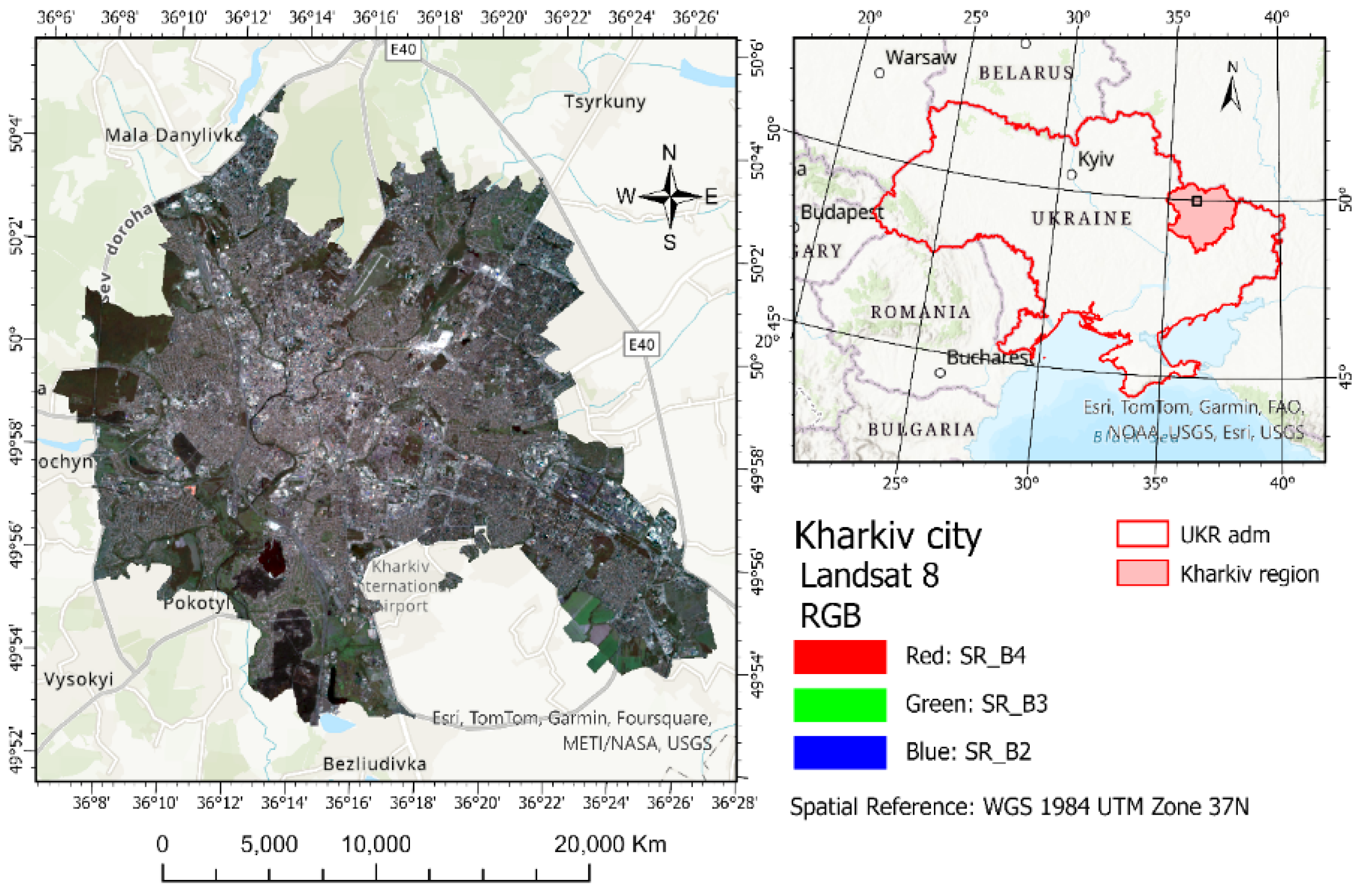
Figure 2.
Monthly average Tair over a 42-year period from CRU TS, Kharkiv Ukraine.
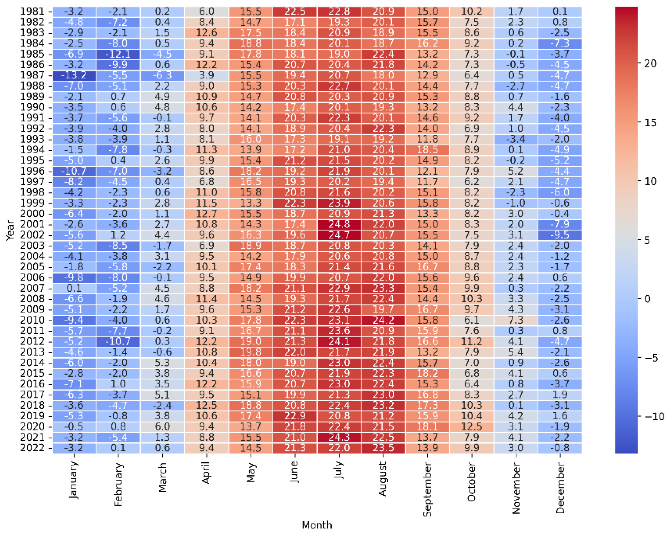
Figure 4.
LST maps for July 1984-2023 based on Landsat.
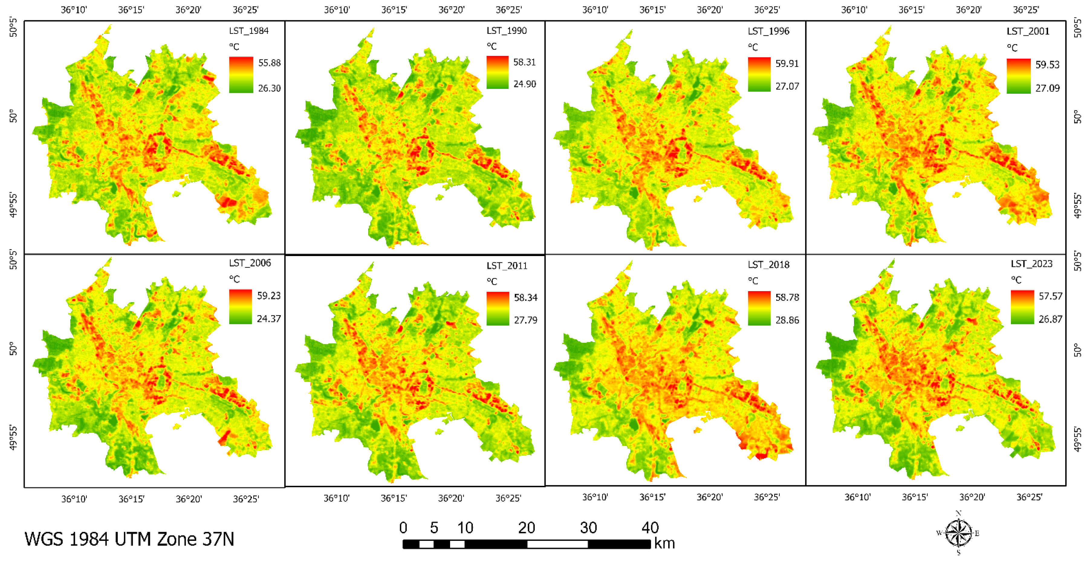
Figure 5.
Mean LST for April-September 1984-2023 based on Landsat.
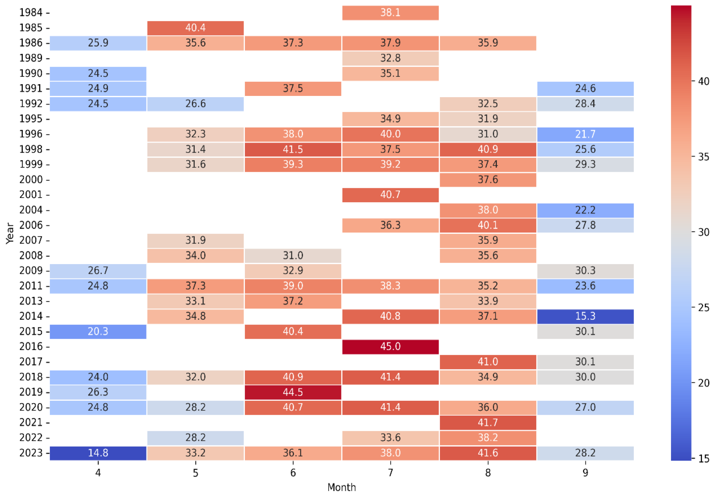
Figure 6.
Mean LST for April-September 1984-2023 based on Modis.
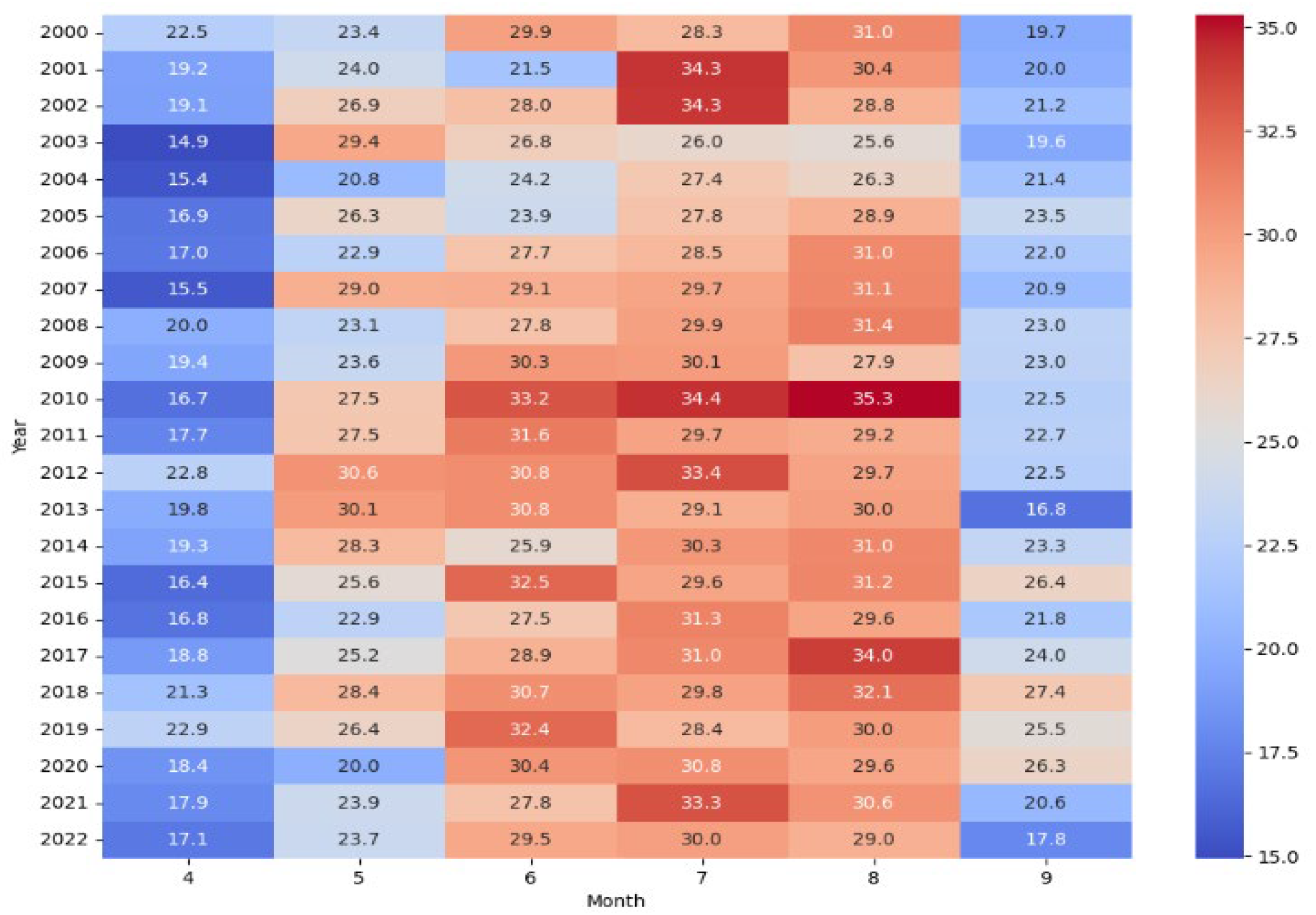
Figure 7.
Linear relationship between Tair and LST values.
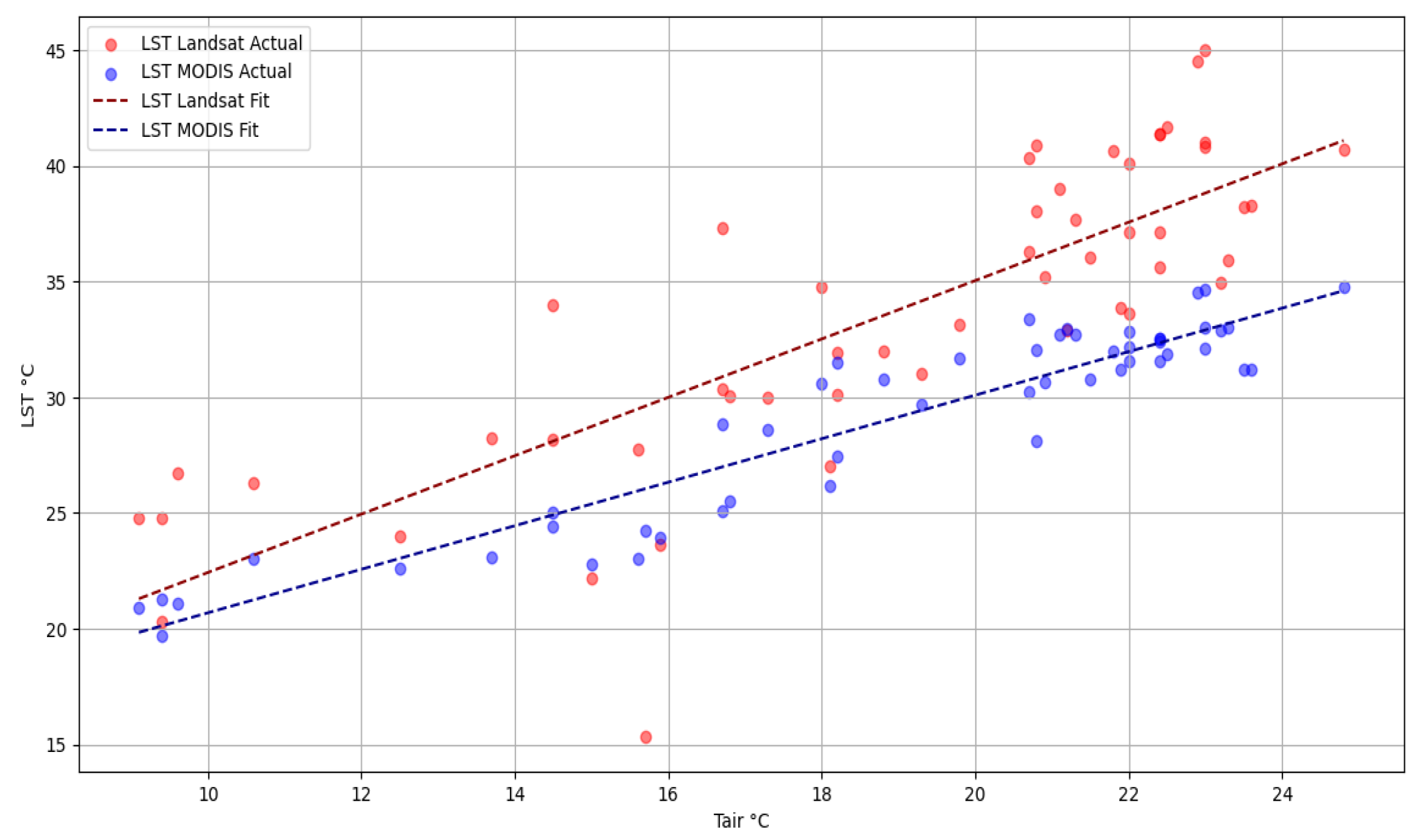
Figure 8.
Dynamics of LULC classes over the years.
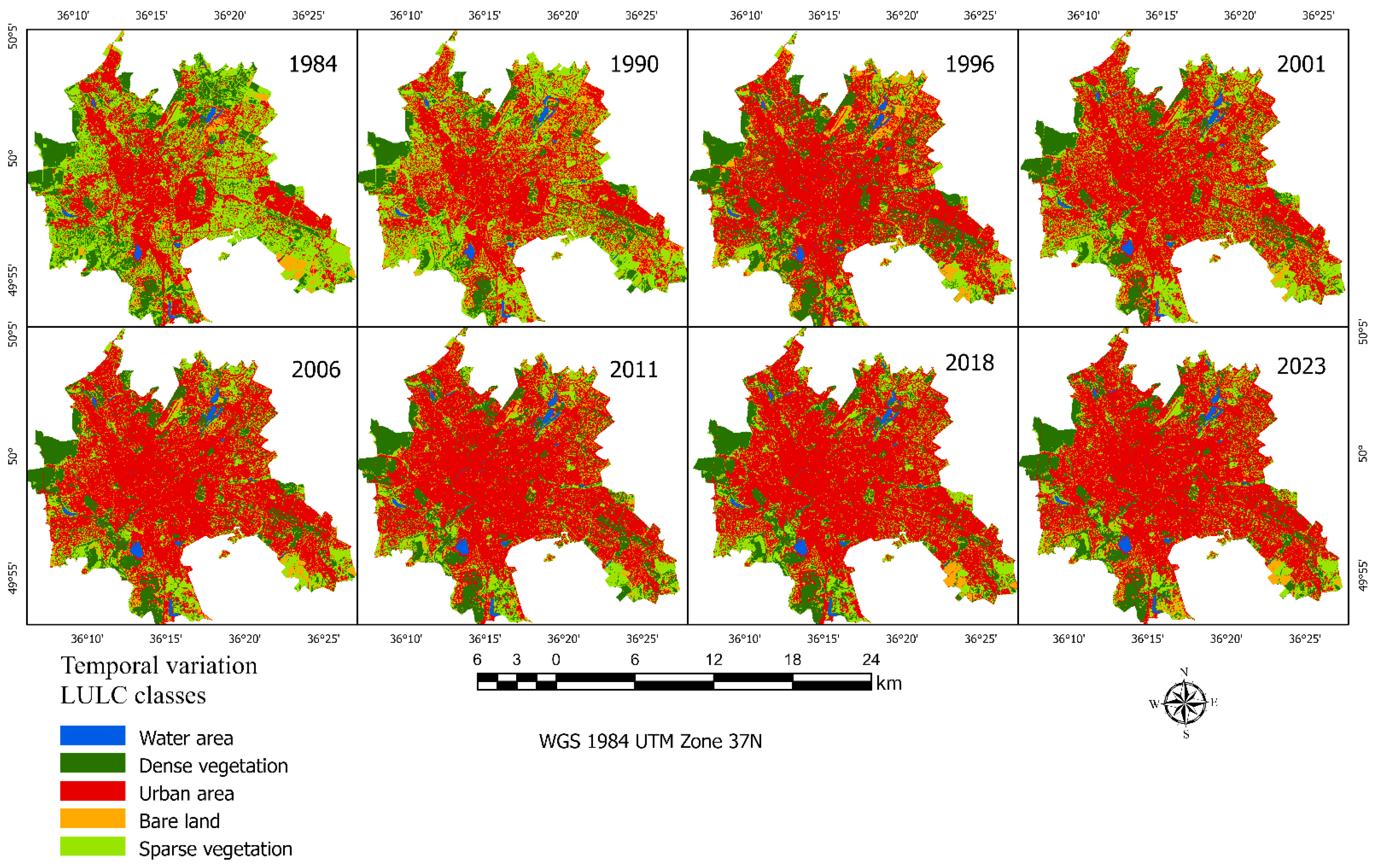
Figure 9.
Change detection between 1984 and 2023.
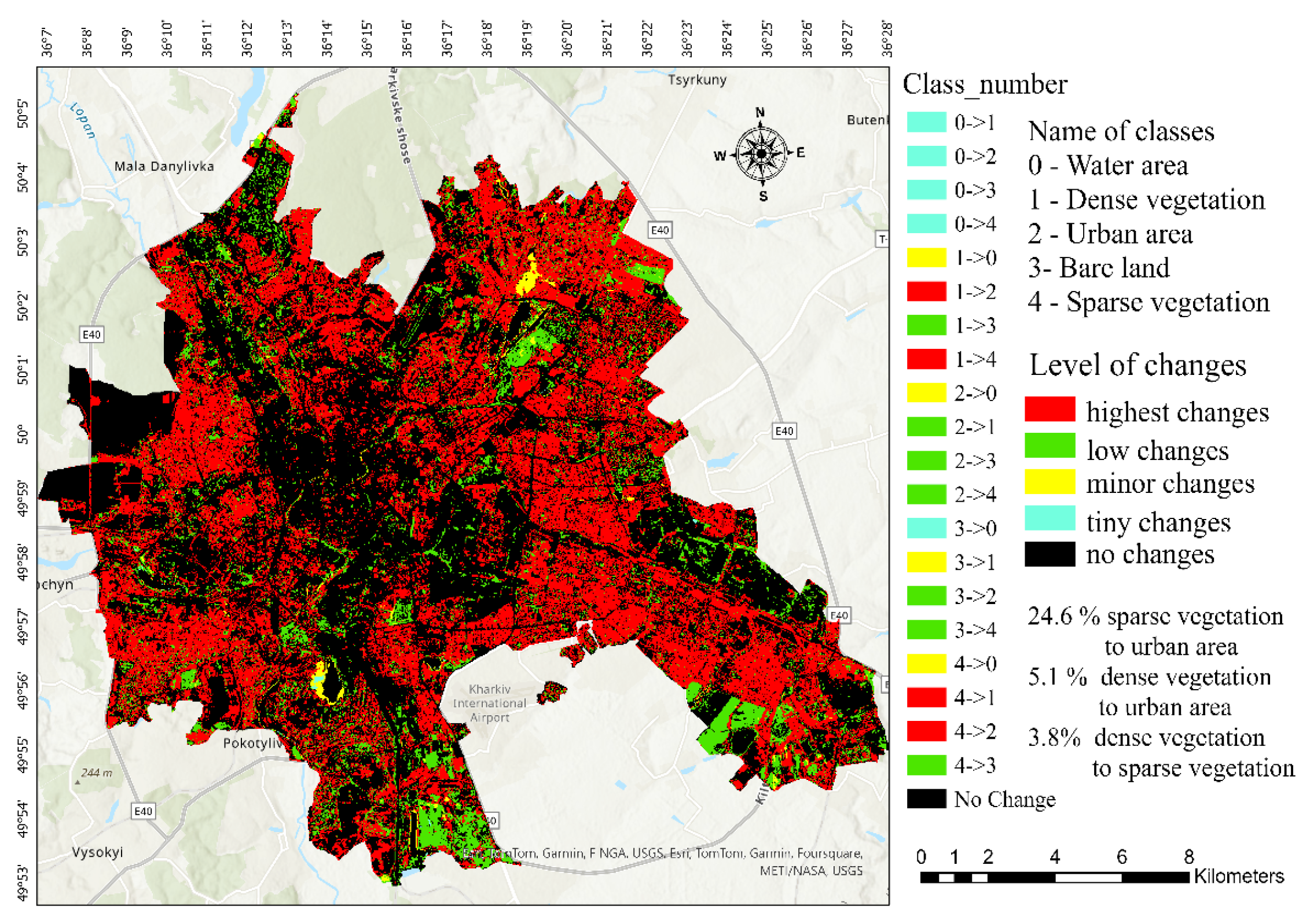
Figure 10.
Relationship between LULC classes and their LST in July a) 1984, b) 2006, c) 2011, d) 2023.
Figure 10.
Relationship between LULC classes and their LST in July a) 1984, b) 2006, c) 2011, d) 2023.
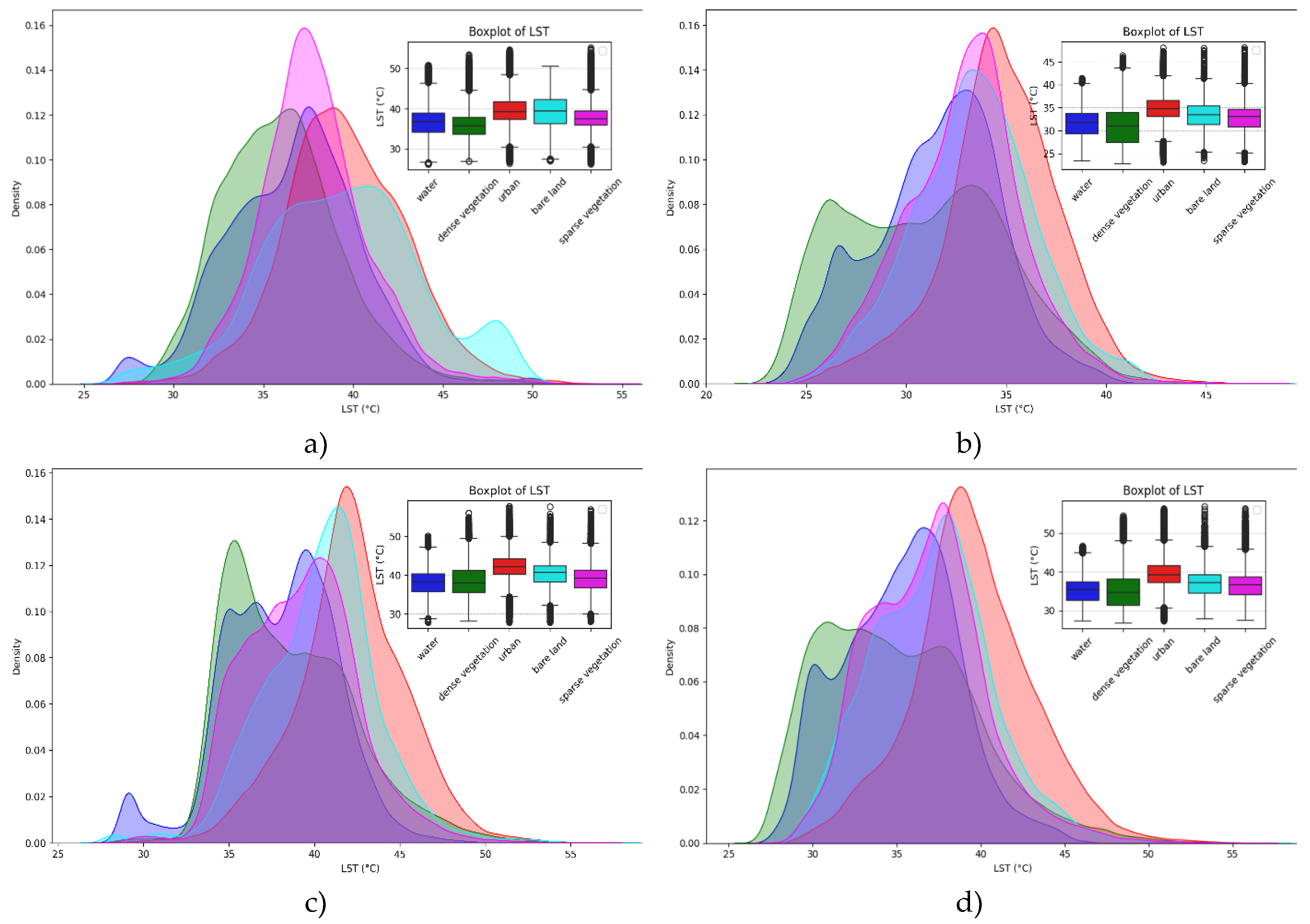
Figure 11.
Quantitative assessment of deviations from normal distribution patterns of LST delineated by average annual values within various LULC classes, based on Shapiro-Wilk and Kolmogorov-Smirnov statistical tests.
Figure 11.
Quantitative assessment of deviations from normal distribution patterns of LST delineated by average annual values within various LULC classes, based on Shapiro-Wilk and Kolmogorov-Smirnov statistical tests.
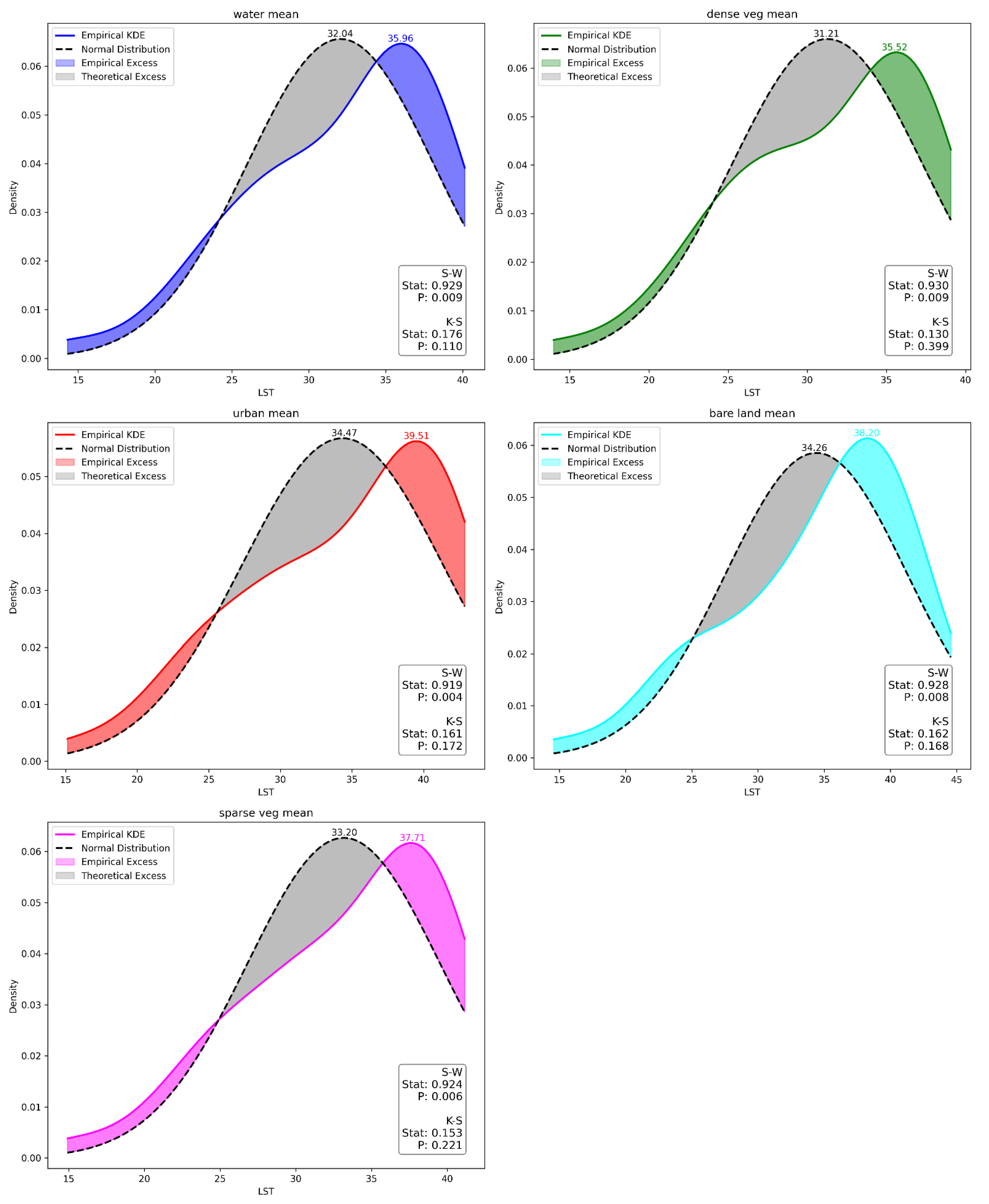
Figure 12.
Quantitative assessment of deviations from normal distribution patterns of LST delineated by average monthly values within various LULC classes, based on Shapiro-Wilk and Kolmogorov-Smirnov statistical tests.
Figure 12.
Quantitative assessment of deviations from normal distribution patterns of LST delineated by average monthly values within various LULC classes, based on Shapiro-Wilk and Kolmogorov-Smirnov statistical tests.
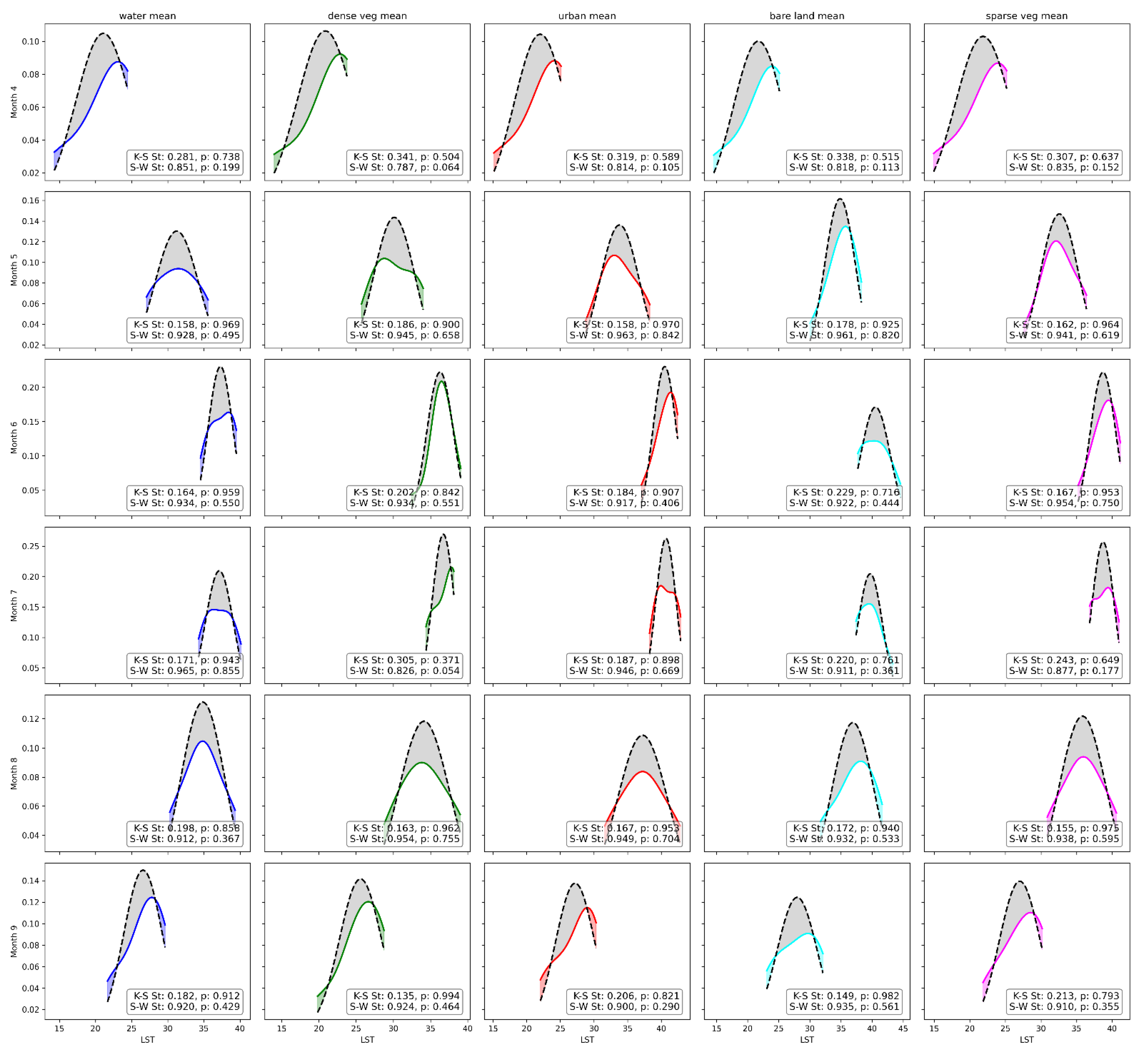
Figure 13.
Comparison of SUHI effect for July a) 1984 and b) 2023.
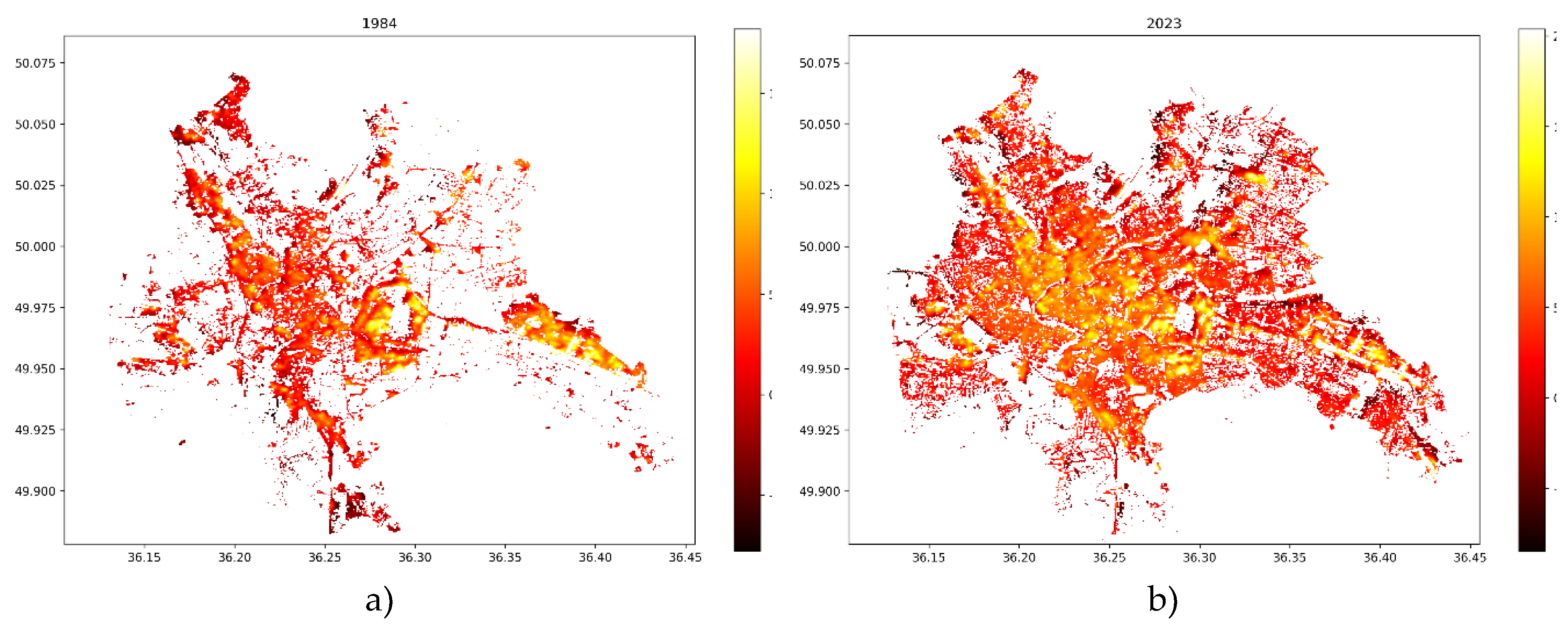
Figure 14.
Urbanization and SUHI Trend in a) July and b) August.
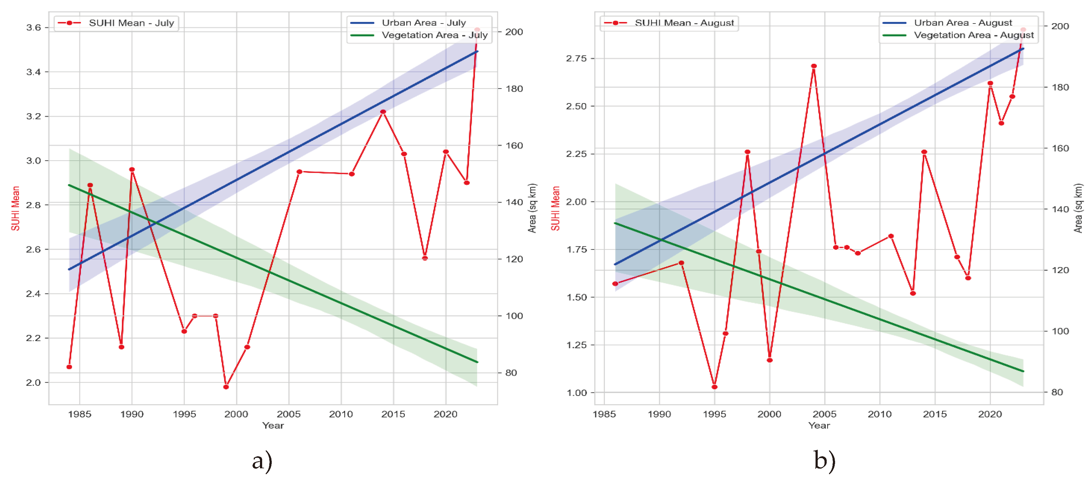

Table 1.
Summary of the datasets in this study.
| Collection/Product | LULC | LST | Cloud % | Period | Total data |
|---|---|---|---|---|---|
| Landsat 5 Level 2, Collection 2, Tier 1 | SR_B1-SR_B7 (30 m) | ST_B6 (100 m) | 0-10 | April-September 1984-2011 |
61 |
| Landsat 8/9 Level 2, Collection 2, Tier 1 | SR_B2-SR_B7 (30 m) | ST_B10 (100 m) | 0-10 | April-September 2012-2023 |
45 |
| MOD11A1.061 | - | LST_Day (1 km) | - | April-September 2000-2022 |
138 |
| CRU TS Version 4.07 | - | Tair | - | Average monthly 1984-2022 |
456 |
Table 2.
LULC classes and training and validation samples.
| Class 1 | Class 2 | Class 3 | Class 4 | Class 5 | |
|---|---|---|---|---|---|
| Type LULC | Water | Dense vegetation | Urban area | Bare land | Sparse vegetation |
| description | rivers, lakes, reservoirs, and other hydrographic features | parks, trees, forests | buildings, roads, and other artificial structures | bare soil and sand | grasslands and shrubs |
| Training samples (1532 elements) | 200 | 209 | 253 (33 polygons) | 200 | 150 |
| Validation samples (376 elements) | 70 | 80 | 97 | 60 | 69 |
Table 3.
Results of linear trend analysis for Tair.
| month | 1 | 2 | 3 | 4 | 5 | 6 | 7 | 8 | 9 | 10 | 11 | 12 | Yearly |
|---|---|---|---|---|---|---|---|---|---|---|---|---|---|
| Slope | 0.009 | 0.076 | 0.066 | 0.036 | 0.023 | 0.059 | 0.059 | 0.074 | 0.045 | 0.029 | 0.082 | 0.063 | 0.052 |
| p-value | 0.788 | 0.077 | 0.057 | 0.119 | 0.292 | 0.003 | 0.001 | 0 | 0.028 | 0.097 | 0.003 | 0.047 | 0 |
| R2 | 0.002 | 0.076 | 0.088 | 0.059 | 0.028 | 0.204 | 0.234 | 0.405 | 0.115 | 0.068 | 0.200 | 0.095 | 0.414 |
| τ | -0.039 | 0.205 | 0.187 | 0.113 | 0.097 | 0.334 | 0.359 | 0.493 | 0.259 | 0.160 | 0.324 | 0.188 | 0.487 |
| p (τ) | 0.712 | 0.056 | 0.083 | 0.298 | 0.368 | 0.002 | 0 | 0 | 0.016 | 0.139 | 0.003 | 0.083 | 0 |
Table 4.
Results of a linear trend analysis for the LST obtained from Landsat.
| month, observations | 4 (11) | 5 (16) | 6 (14) | 7 (17) | 8 (20) | 9 (15) |
|---|---|---|---|---|---|---|
| Slope | -0.102 | -0.089 | 0.052 | 0.091 | 0.133 | 0.071 |
| p-value | 0.199 | 0.246 | 0.545 | 0.131 | 0.042 | 0.531 |
| R2 | 0.176 | 0.102 | 0.031 | 0.146 | 0.213 | 0.031 |
| τ | -0.273 | -0.124 | 0.231 | 0.309 | 0.295 | 0.181 |
| p (τ) | 0.283 | 0.559 | 0.279 | 0.091 | 0.074 | 0.380 |
Table 5.
Results of a linear trend analysis for the LST based on Modis.
| Month | 4 | 5 | 6 | 7 | 8 | 9 |
|---|---|---|---|---|---|---|
| Slope | 0.045 | -0.019 | 0.203 | 0.043 | 0.083 | 0.131 |
| p-value | 0.545 | 0.844 | 0.023 | 0.567 | 0.221 | 0.116 |
| R2 | 0.018 | 0.002 | 0.222 | 0.016 | 0.071 | 0.113 |
| τ | 0.107 | -0.004 | 0.281 | 0.209 | 0.170 | 0.304 |
| p (τ) | 0.497 | 1 | 0.064 | 0.172 | 0.271 | 0.044 |
Table 6.
Results of linear regression between Tair and LST based on Landsat and Modis.
| Slope | Intercept | R2 | p-value | τ | RMSE | |
|---|---|---|---|---|---|---|
| LST Landsat | 1.261 | 9.82 | 0.663 | 2.18×10⁻¹³ | 0.626 | 3.815 |
| LST MODIS | 0.94 | 11.289 | 0.879 | 1.27×10⁻²⁴ | 0.711 | 1.476 |
Table 7.
Accuracy assessment of classification results.
| July, Year | 1984 | 1990 | 1996 | 2001 | 2006 | 2011 | 2018 | 2023 | ||||||||
|---|---|---|---|---|---|---|---|---|---|---|---|---|---|---|---|---|
| Class | UA | PA | UA | PA | UA | PA | UA | PA | UA | PA | UA | PA | UA | PA | UA | PA |
| Water | 1 | 1 | 1 | 1 | 1 | 1 | 1 | 0.98 | 1 | 1 | 1 | 1 | 1 | 0.99 | 1 | 0.99 |
| Dense veg | 0.88 | 0.99 | 0.95 | 0.9 | 0.96 | 0.95 | 0.96 | 0.93 | 0.94 | 0.77 | 0.86 | 0.89 | 0.87 | 0.74 | 0.88 | 0.9 |
| Urban area | 0.98 | 0.95 | 0.99 | 0.96 | 0.99 | 0.94 | 0.99 | 0.96 | 0.98 | 1 | 0.91 | 1 | 0.72 | 1 | 0.93 | 0.95 |
| Bare land | 0.83 | 0.83 | 0.94 | 0.75 | 0.91 | 0.98 | 0.86 | 0.9 | 0.94 | 0.73 | 0.85 | 0.85 | 0.96 | 0.82 | 0.78 | 0.98 |
| Sparse veg | 0.81 | 0.73 | 0.71 | 0.9 | 0.92 | 0.94 | 0.89 | 0.91 | 0.64 | 0.87 | 0.76 | 0.64 | 0.8 | 0.63 | 0.87 | 0.67 |
| OA | 0.91 | 0.91 | 0.95 | 0.94 | 0.89 | 0.88 | 0.84 | 0.9 | ||||||||
| Kappa | 0.88 | 0.89 | 0.94 | 0.92 | 0.85 | 0.85 | 0.8 | 0.87 | ||||||||
Table 8.
Dynamics of LST changes by LULC classes: analysis of mode, median, variability, and extreme values.
Table 8.
Dynamics of LST changes by LULC classes: analysis of mode, median, variability, and extreme values.
| Year | Class | Mode | Med | IQR | Min | Max | Out | Sp | Sk | MM |
|---|---|---|---|---|---|---|---|---|---|---|
| 2023 | water | 30.1, 36.59 | 35.38 | 4.92 | 27.49 | 46.67 | 52 | 16.51 | 0.1 | 2 |
| 1984 | water | 27.49, 37.51, 47.48, 49.86 | 36.93 | 4.91 | 26.31 | 50.85 | 194 | 17.66 | 0.05 | 4 |
| 2023 | dense veg | 30.88, 32.71, 37.59, 52.85 | 34.65 | 6.69 | 26.88 | 54.59 | 354 | 20.92 | 0.61 | 4 |
| 1984 | dense veg | 36.51, 48.26 | 35.83 | 4.37 | 27.03 | 53.4 | 768 | 15.6 | 0.58 | 2 |
| 2023 | urban | 38.8 | 39.3 | 4.39 | 27.42 | 56.28 | 4194 | 17.68 | 0.18 | 1 |
| 1984 | urban | 28.22, 38.88 | 39.39 | 4.49 | 26.42 | 54.66 | 1600 | 16.4 | 0.13 | 2 |
| 2023 | bare land | 37.97, 51.49, 54.24 | 37.23 | 4.85 | 27.96 | 56.87 | 123 | 16.73 | 0.4 | 3 |
| 1984 | bare land | 40.81, 47.91 | 39.4 | 5.89 | 27.09 | 50.68 | 40 | 23.02 | -0.02 | 2 |
| 2023 | sparse veg | 34.23, 37.73, 51.49, 52.97, 54.36 | 36.77 | 4.7 | 27.55 | 56.44 | 616 | 16.71 | 0.55 | 5 |
| 1984 | sparse veg | 27.18, 37.25, 47.78, 53.4, 54.59 | 37.59 | 3.57 | 26.31 | 55.14 | 3099 | 13.68 | 0.51 | 5 |
Table 9.
Thresholds of different LULC classes based on Landsat LST over the years.
| Class | Med LST | Lower Threshold (LT) | Upper Threshold (UT) | St.dev. |
|---|---|---|---|---|
| bare land | 38.20 | 32.47 | 45.49 | 2.45 |
| dense veg | 35.52 | 27.41 | 45.45 | 2.24 |
| sparse veg | 37.71 | 31.93 | 44.44 | 2.16 |
| urban | 39.51 | 33.48 | 46.51 | 2.09 |
| water | 35.96 | 29.61 | 44.65 | 2.29 |
Table 10.
Seasonal LST thresholds for different LULC classes for different years.
| month | water mean | dense veg. mean |
urban mean | bare land mean |
sparse veg. mean |
water LT | water UT | dense veg. LT |
dense veg. UT |
urban LT | urban UT | bare land LT |
bare land UT |
sparse veg. LT |
sparse veg. UT |
|---|---|---|---|---|---|---|---|---|---|---|---|---|---|---|---|
| 4 | 21.09 | 20.85 | 22.00 | 21.73 | 21.82 | 14.74 | 27.43 | 15.7 | 26.01 | 17.57 | 26.42 | 17.15 | 26.31 | 17.41 | 26.31 |
| 5 | 31.24 | 30.12 | 33.8 | 34.85 | 32.58 | 23.05 | 39.43 | 22.18 | 38.07 | 27.53 | 40.07 | 27.01 | 42.65 | 25.95 | 39.2 |
| 6 | 37.29 | 36.28 | 40.5 | 40.54 | 38.75 | 28.64 | 45.94 | 27.64 | 44.93 | 33.58 | 47.41 | 32.32 | 48.76 | 31.55 | 45.86 |
| 7 | 37.13 | 36.71 | 40.69 | 39.69 | 38.72 | 29.85 | 44.42 | 28.62 | 44.8 | 33.83 | 47.54 | 32.76 | 46.62 | 32.17 | 45.25 |
| 8 | 34.85 | 34.12 | 37.21 | 36.91 | 35.83 | 28.18 | 41.52 | 27.39 | 40.85 | 31.36 | 43.05 | 30.24 | 43.58 | 30.19 | 41.45 |
| 9 | 26.58 | 25.58 | 27.19 | 27.95 | 27.02 | 20.73 | 32.45 | 20.76 | 30.4 | 23.12 | 31.26 | 22.7 | 33.21 | 22.52 | 31.55 |
* LT – lower threshold, UT – upper threshold.
Table 11.
Correlation analysis between SUHI mean and indicators in July and August.
| July | rx,y | p (rx,y ) | ρ | p (ρ) | τ | p (τ) |
|---|---|---|---|---|---|---|
| SUHI mean and LST mean | 0.167 | 0.521 | 0.236 | 0.359 | 0.141 | 0.432 |
| SUHI mean and Tair | -0.113 | 0.664 | -0.065 | 0.804 | -0.052 | 0.772 |
| SUHI mean and urban area | 0.511 | 0.035 | 0.581 | 0.014 | 0.421 | 0.02 |
| SUHI mean and vegetation area | -0.442 | 0.075 | -0.59 | 0.012 | -0.439 | 0.016 |
| August | ||||||
| SUHI mean and LST mean | 0.559 | 0.01 | 0.585 | 0.007 | 0.423 | 0.009 |
| SUHI mean and Tair | 0.406 | 0.076 | 0.415 | 0.069 | 0.296 | 0.069 |
| SUHI mean and urban area | 0.539 | 0.014 | 0.518 | 0.019 | 0.405 | 0.014 |
| SUHI mean and vegetation area | -0.605 | 0.005 | -0.515 | 0.02 | -0.416 | 0.012 |
Table 12.
Results of a linear trend analysis for SUHI in July and August.
| July | Slope | Intercept | R2 | p-value | SE | τ | p (τ) |
|---|---|---|---|---|---|---|---|
| SUHI mean | 0.022 | -43.254 | 0.409 | 0.005 | 0.007 | 0.459 | 0.01 |
| August | |||||||
| SUHI mean | 0.028 | -54.647 | 0.345 | 0.006 | 0.009 | 0.423 | 0.009 |
Disclaimer/Publisher’s Note: The statements, opinions and data contained in all publications are solely those of the individual author(s) and contributor(s) and not of MDPI and/or the editor(s). MDPI and/or the editor(s) disclaim responsibility for any injury to people or property resulting from any ideas, methods, instructions or products referred to in the content. |
© 2024 by the authors. Licensee MDPI, Basel, Switzerland. This article is an open access article distributed under the terms and conditions of the Creative Commons Attribution (CC BY) license (http://creativecommons.org/licenses/by/4.0/).
Copyright: This open access article is published under a Creative Commons CC BY 4.0 license, which permit the free download, distribution, and reuse, provided that the author and preprint are cited in any reuse.


