
Submitted:
10 October 2025
Posted:
13 October 2025
You are already at the latest version
Abstract
Home range size and habitat selection of two kin-related female wild boars belonging to the same family group were analysed within an area of 8,6 km2 in the Apennine Mountains (Central Italy). Changes in home range size, spatial overlap, and habitat preferences were analysed using a very high frequency (VHF) telemetry data, across three distinct stages of the reproductive period: before, during, and after births. Our results show a marked reduction in home range size during the farrowing phase suggesting a behavioural shift towards more restricted space likely associated with reproductive constraints. A spatial overlap between the two females peaked during the farrowing period and it was followed by sharp post-births decrease, implying a temporary spatial convergence linked to a common selection of suitable birthing site. During and after farrowing, both individuals/females showed a non-random dispersal pattern, selecting areas characterized by dense vegetation and lower/minimal anthropogenic disturbance. Distances from the core centres of activity varied significantly across the three phases, reflecting changes in mobility strategies. These results highlight the influence of the reproductive status on spatial behaviour in female wild boar and underscore the importance of a fine-scale temporal analysis to detect patterns of habitat selection and social spacing within family groups. Our study contributes to a better understanding of wild boar ecology in Apennine landscapes, with implications for future research in this widespread and adaptable species.
Keywords:
wild boar
; radiotracking
; spatial analysis
; home range
; reproductive behaviour
1. Introduction
The definition of home range is still widely accepted: an area crossed by an animal during its normal foraging activities, mating and parental care [1]. Later studies refined this concept by emphasising its ecological and social dimensions, highlighting that the home range not only reflects resource distribution but also the spatial strategies animals adopt to meet reproductive and survival needs [2]. In addition, analysing the degree of spatial overlap among individuals provides valuable insights into social organisation, competition, and cooperative behaviours, especially in group-living species such as wild boar [3,4]. Sex- and group-specific home ranges of wild boars have been reported in Italy [5]: adult males’ range between 870 and 1,750 hectares, adult females between 360 and 560 hectares, while family groups of similarly aged individuals can reach up to 2,400 hectares. More fine-scale evidence was provided by a radiotracking study on adult wild boars in the Maremma Natural Park (Central Italy), which highlighted relatively small daily home ranges and a consistent pattern of activity concentrated during twilight and nighttime hours; the study did not detect differences between sexes or across months, a result likely influenced by the absence of breeding females and of significant human disturbance in the area, conditions that may also account for the higher degree of diurnally observed compared to other populations [6]. These differences in space use reflect distinct reproductive strategies of males and female, which are in turn associated with the concept of allometric scaling of spatial requirements [7,8]. Seasonal changes in behavioural and the environmental conditions affect spatial dynamics and may influence inter- and intra-species interactions [9,10], home range size and habitat use [9,11]. Variation in spatial interactions between individuals may reveal selective pressures shaping spatial use [12]; such dynamics are influenced by a combination of behavioural traits and environmental variables, which in turn affect spatial organisation within a population. The specific interactions influence the individual spatial pattern and these drive population processes such as disease transmission [13], reproduction [14], survival [15,16] and competition [17]. Despite the growing trend that spatial relationships influence different socio-ecological processes [18], variation in spatial patterns between sexes and age is poorly understood for wild boar in Apennine Mountains and identifying factors influencing this heterogeneity in spatial pattern can improve management and conservation decisions, including disease transmission [19], intraspecific competition [17] and management actions [20]. Uncovering the factors influencing spatial overlap heterogeneity can refine ecological knowledge and improve conservation planning, especially during critical phases such as farrowing and early parental care. To improve understanding of spatial ecology and home range dynamics of wild boar, we conducted a telemetry study on pregnant wild boar females from March to June to assess space use during farrowing and early postnatal periods.
2. Material and Methods
2.1. Study Area
The study area (latitude 43° 3.006’ N; longitude 13° 6.373’ E) lies at altitudes between 450 and 890 m with and average altitude of 675,8 m above sea level, belongs to the Umbria-Marche Apennines (Figure 1A) and consists of sedimentary rock formations spanning from the Lower Jurassic (200 Ma) to the Upper Miocene (5 Ma). The region is shaped by fold and thrust fault tectonics. The landscape consists of foothills transitioning between cultivated land, forests, and secondary grassland; the vegetation communities include Downy Oak Forests (Quercus pubescens), Hornbeam Forests (Ostrya carpinifolia), Holm Oak Forests (Quercus ilex), grassland and cultivated land; forests occupy 47% of the land, mainly composed of oak and hornbeam, while the remaining percentage consists of agricultural areas, shrubland and grassland (Table 1). The study area borders the Sibillini National Park for 6.5 km, creating a complex conservation and management scenario; the protected area serves as a wildlife reservoir, influencing species dynamics on a much smaller scale and in much larger territories than our study area. For the entire period of the research, wild boar hunting was closed.
2.2. Data Collection
Preliminary surveys were carried out counting wild boar tracks and some direct observation sessions at dusk; eight females of reproductive age were counted with a few young specimens. The group of females showed some stability in frequenting the study area during the preliminary observations; within this group there was a particularly robust female who preceded the group's movements in the various sightings: we hypothesise that she may be the leading female. The movement of two wild boar adult females was investigated by VHF telemetry study; to catch the subjects we built a trap-cage with wood and electro-welded mesh (15 × 15 cm) for a total size of 5 × 2 × 2 meters. The bottom of the cage was without a net to mitigate the subjects' wariness to cross the trap. The trap activation system was designed to prevent the capture of non-target species, and we used corn as bait for capturing. The locking device was made at a height compatible with that of the subjects to be captured. The trigger force was around 1.5 kg. The trap was provided with an MMS function camera for capturing subjects and was equipped of lateral small manipulation cage to allow the operator for marking animals. Ensuring that handling activities were stress-free, the subjects were lightly sedated because the weight of the boars captured exceeded the 65 kg. A solution of azaperone and tiletamine/zolazepam was injected intramuscularly in the femoral region with 5 ml anaesthetic darts using a blowpipe (a 14mm diameter and 1.5m long aluminum tube). The weight was estimate of each animal in the trap. The estimated final dosage was 2mg/kg of azaperone and 0.75/0.75 mg/kg of tiletamine/zolazepam [21,22].
The first boar was caught on 19 March 2015; this female was the largest female of the group following a photo comparison. The subject was reached at 9:45 am and the anaesthetic was given; the injection was performed in hind legs and after 15 minutes the boar was released with Telenax ear lobe radio tag (Telenax 239VHF e G102) with the nickname “Hermione”; we have chosen the ear transmitters tags as they were successfully used in numerous telemetry studies of deer and other ungulates [23]. Each brand weighted 20.5 grams with a range of 25 km and one year of autonomy. The second boar was caught on 21 March 2015; this female was also declared pregnant, was treated with the same anaesthetic procedure of the previous one and was released with ear lobe radio tag (Telenax 319VHF e G104) with the nickname “Farukka”. To increase the visibility of the marked subjects, two high-visibility brands in each ear subjects were applied.
The position of the animals was determined with a receiving station (frequencies from 152.000 to 153.200 Mhz) and a three-element Yagi antenna. The direction of the signal was achieved by the strongest signal method [24,25] while the position was determined using the triangulation method; for this purpose, 23 VHF receiving stations were identified in the study area (Figure 1B). The subjects were followed weekly in sections of six hours: 00.00 – 06:00; 06:00 – 12:00; 12:00 – 18:00; 18:00 – 24:00; each fix was given by date, time, tracking station, subject and compass directions. VHF monitoring started on March 22nd and ended on June 30th when devices stopped transmitting the signal.
On April 22th the subjects captured and marked were observed and photographed with four (Farukka) and seven (Hermione) respectively young striated boars; thanks to these observations we were able to divide the observations into three period: first period (50 fixes), named pre-birth phase, from March 22th to April 20th; second period (35 fixes), named birth phase, from April 21th to May 15th, third period, named post-birth phase (30 fixes) after May 15th.
2.3. Data Analysis
The extent of the spatial dataset is a bounding box (axis-aligned), the smallest rectangle (856,4 hectares) that contain all the VHF receiving station dataset (Figure 1B). As a first step of our analysis, we aimed to evaluate whether wild boar localizations followed a random spatial pattern or whether they exhibited signs of clustering. To this purpose, we tested the hypothesis of complete spatial randomness (CSR), which represents the simplest theoretical model of spatial point processes. CSR assumes that events have an equal likelihood of occurring anywhere within the study area, independent of the locations of other events, and is formally represented by a homogeneous Poisson process [26]. While most ecological processes tend to deviate from CSR to some degree, assessing this model is a crucial starting point because it allows distinguishing between regular and clustered patterns. In a random distribution, the occurrence of each point is independent of the others, with neither attraction nor inhibition. In contrast, regular patterns are characterized by greater spacing between points than expected under randomness, often due to competitive mechanisms that limit proximity. Clustered patterns, instead, show higher aggregation of points, a condition typically associated with processes such as reproduction with limited dispersal or the influence of environmental heterogeneity.
Since the individuation of VHF fix position is less precise than it would be with GPS devices, we tested CSR using χ2 test based on quadrat counts; this method relies on the fact that, under CSR, the expected number of observations within any region of equal size is the same. The quadrat method evaluates whether the CSR is reasonable by comparing the observed value of the χ2 statistic to the χ2m−1 distribution, where m is the number of squares. The significance was assessed using Monte Carlo, which involves generating multiple models under the null hypothesis and calculating the value χ2 statistic for each of them. The p-value is then determined by comparing the χ2 statistic for the observed point pattern with the χ2 values obtained from the simulations. The number of quadrats was defined using the test for independence of all factors and choosing the highest number of quadrats with statistic lower than the χ2 value for given degrees of freedom; the best configuration was a 5 × 5 grid (Figure 2) for a total of 25 quadrants and 230 fixes (χ2 = 29.581; df = 16; p-value = 0.0203).
To describe the distribution of two female across different land cover types, we calculated the breadth of habitat use using the Levin’s normalized index (L) [27] and the overlap in habitat use with Pianka's index (Ojk) [28], based on the proportion of contacts in each land cover type. In addition, geometric overlap of the individuals’ location was assessed using the Bhattacharyya affinity index [4] based on grid cells.
The home range analysis [1,2,3,4,5,6,7,29,30,31,32,33,34,35,36,37,38,39,40,41] was carried out using the Minimum Convex Polygon (MCP) estimation method. The MCP method consists in the calculation of the smallest polygon enclosing all the relocations of the animal; because the home range has been defined as the area transversed by the animal during its normal activities of foraging, mating and caring for young [1], we computed thee home-range size for various choices of the number of extreme relocations to be excluded. We estimated the home ranges for the three births phases using the Adehabitat R [42] package for RStudio version 1.4.1717 [43].
2.4. Environmental Analysis
Habitat selection by female wild boars was assessed using the Jacobs Selection Index [44], which ranges from –1 (total avoidance) to +1 (total selection), with values around zero indicating use proportional to availability. This index compensates for extreme differences between use and availability and if a habitat is very abundant but little used, Jacobs will clearly show it as avoided and allows you to evaluate multiple habitats in the same context. For this analysis eleven parameters were collected using QGIS 3.28.15 geoprocessing tools; for each location a 100 meter buffer was created and for each buffer the vegetation parameters were measured. Vegetation parameters were totally collected through field surveys and are expressed as proportion (p) of habitat available in the study area. Parameters were analyzed using two independent samples t test; the response variables were the three stages (pre-birth, birth and post-birth), while the predictors were the two-level categorical variable wild boar females. If the distribution was not normal the non-parametric Wilcoxon Mann-Whitney test (U) was applied [45]. All statistical analyses were performed in RStudio 1.4.1717 [43], using R [42] stats package; the significance level was set at α = 0.05 for all tests.
3. Results
3.1. Complete Spatial Randomness (CSR) Analysis
The quadrat method (χ2 = 497.61, p-value = 0.000) reject the null hypothesis of complete spatial randomness; the wild boars exhibit a strong clustered pattern. A clustered pattern is also present if we carry out the tests for the Farukka (χ2 = 327.83, p-value = 0.000) and Hermione (χ2 = 268.26, p-value = 0.000) localizations (Figure 2). Dispersal distances are very low; the two female wild boars had average dispersal distances ranging between 550 and 650 m, with maximum values not exceeding 2 km from the capture site (Table 2).
The analysis of dispersal distances from the capture site showed no significant difference between the two females (Wilcoxon rank-sum test: W = 6703, p = 0.858). Hermione’s fixes have an interquartile range (IQR) of 370.3 m (Q1 = 385.5 m; Q3 = 755.8 m), while Farukka’s ones spanned a broader range, from 65.9 to 1,648.9 meters, with a larger IQR of 571.7 m (Q1 = 310.9 m; Q3 = 882.6 m). Although Farukka exhibited slightly higher mean and maximum distances, as well as a wider variability, the strong overlap between the two distributions (Figure 2) suggests that both females displayed broadly similar dispersal patterns from the capture site.
3.2. Home Range Analysis
Home range (HR) values were measured using the minimum convex polygon method (MCP) at various percentile levels representing different extent of their home range. The two females exhibit slightly different overall dispersal behaviours (Figure 3): Hermione seems to be more territorial, with a home range varying from a minimum of 51.3 ha (MCP50) to a maximum of 146.8 ha (MCP100). On the other hand, Farukka displays a broader dispersal pattern, with minimum home range values comparable to those of Hermione (41.9 ha MCP50) but significantly larger maximum values (287.3 ha MCP100).
The comparative analysis of the HR size at percentile levels shows a difference in spatial behaviour between the two females across three distinct phases (Table 3). The data reveal differences in the HR of Farukka and Hermione before births; for Hermione, the HR ranges from 49.7 hectares at the 50th percentile to 121.6 hectares at the 100th percentile, in contrast, Farukka exhibits a considerably larger HR, ranging from 125.5 hectares at the 50th percentile to 275.0 hectares at the 100th percentile. This indicates that Farukka has a more extensive home range compared to Hermione before giving birth, suggesting a possible difference in individual ranking and relative territorial or foraging behaviour. During the birthing phase both females exhibit a reduction of over 50% in their home range sizes, which could be attributed to the increased need for proximity to birthing sites and reduced mobility. The post-birth data suggest that both females slightly expand their home range (approximately 20-30% of the size observed during births), but this does not suggest a return to the normal activities observed before births; Hermione exhibits a greater expansion compared to Farukka (Table 3).
The Table 4 presents the breadth (Levin’s index), overlap (Pianka’s index) of habitat uses and distributions affinity indices for both females (Bhattacharyya index), across the three different temporal phases. The breadth in habitat use of Hermione shows variations across the different phases, with the lowest values occurring during births (L=0.11); this indicates a marginally narrower and potentially more specific resources utilization during the birthing period. This situation seems to be temporary because Hermione in the post-birth phase increases the use of landcover type with values higher than that pre-birth phase. Conversely, Farukka exhibits a noticeable reduction in habitat use during and after births (L=0.12 and L=0.13, respectively), suggesting a more constrained resources utilization during these times compared to the pre-birth period (L=0.17). The Pianka’s overlap index (Table 4) indicates significant temporal fluctuations between the two wild boar females; the overlap is highest during pre-birth phase (Ohf=0.87), nearly complete, suggesting a common preference for specific resources during this critical period (Figure 4B). During births and in the post-birth phase the overlap is moderate (Ohf=0.58 and Ohf=0.52 respectively), indicating that when the geometric overlap is maximum due to births and parental care (0.91 and 0.81) the females still partially differentiate the habitat use (Figure 4A) to optimize trophic resources by minimizing interspecific competition. After giving birth, spatial overlap values decrease slightly but remain quite high (0.81), but Hermione, the dominant female, significantly increases the breadth of her landcover type, exceeding the pre-giving birth values. Farukka, subordinate in the rank, shows a post-giving situation very similar to that of giving birth.
In conclusion, the analysis reveals that both females, adjust their spatial breadth based on temporal changes, particularly around the birthing period; these variations appear to be partly determined by the social rank they occupy in the population. Hermione maintains a relatively consistent breadth values throughout, while Farukka's spatial occupancy becomes notably restricted during and after births. The near-complete overlap during births suggests a low degree of spatial competition or shared spatial requirements during this critical period. Finally, it is important to note that the maximum Pianka values are observed when geometric overlap is minimal; this indicates that, always, the two females reduce intraspecific competition to a minimum: in the pre-partum phase the overlap in habitat use is maximum, which indicates that they exploit the same resources, but most of the time in different spaces (Fig. 4A).
3.3. Environmental Analysis
Differences in landcover composition were observed between the two females, confirming variations in habitat use strategies; before births, Farukka and Hermione (Table 5 and Table 6) primarily utilized crops and Hornbeam Forest, but Farukka exhibited a greater reliance on permanent meadows (10.8 ± 4.2%) compared to Hermione (0.2 ± 0.2%, Wilcoxon W = 1,095, p < 0.01), while Hermione had a significantly higher presence in grassland (5.7 ± 1.9%, Wilcoxon W = 1,101, p < 0.01).
During the birthing phase, no differences in the frequency of vegetation types are observed; both females seem to prefer Hornbeam Forest and riverside forests.
After births, the two individuals displayed divergent habitat selection strategies; Farukka increased its reliance on permanent meadows (22.4 ± 5.4%) compared to Hermione (0%), marking a significant shift from the birth period (Wilcoxon W = 273, p < 0.001). In contrast, Hermione showed an increased preference for Broom shrubland (25.5 ± 7.1%, Wilcoxon W = 336, p < 0.001), likely due to the need for denser cover post-births. Hornbeam forest uses significantly decreased for Hermione (19.9 ± 5.8%), whereas Farukka continued selecting this habitat (48.8 ± 7.4%, Wilcoxon W = 343, p< 0.01). Pastures were significantly more used by Hermione (3.3 ± 1.6%) compared to Farukka, where they were completely absent (Wilcoxon W = 367, p < 0.01).
Habitat selection analysis based on Jacobs’ Index [44] revealed distinct patterns of preference across the three phenological stages. During the birth period, a clear shift in habitat selection was observed, with both individuals increasing their use of Hornbeam Forest (D = 0.2870 for Farukka and D = 0.3362 for Hermione) but riverside vegetation became selected by both individuals (D = 0.6918 for Farukka and D = 0.6748 for Hermione), indicating its importance during births (Table 7 and Table 8). The use of crops significantly declined (Table 5 and Table 6) compared to the pre-birth period, dropping to 13.9 ± 3.5% (p < 0.01) for Farukka and 12.6 ± 3.0% for Hermione, reinforcing a transition away from open agricultural areas.
Key results from Jacobs’ Index for births: riparian vegetation, initially avoided, became one of the most strongly selected habitats (D = 0.6918 for Farukka, D = 0.6748 for Hermione, p < 0.001); crops continued to be avoided (-0.4835 for Farukka, -0.5239 and for Hermione) and Pre-wood forests remained strongly avoided (-0.9701 for Farukka, -0.9649 for Hermione, p < 0.001). Both individuals strongly avoided urban areas (Table 7 and Table 8); crops were used by Farukka (D = 0.0430), whereas Hermione slightly avoided them (-0.3376, p < 0.05). Farukka strongly avoided riparian vegetation (-0.9839), while Hermione also showed strong avoidance (-0.9887), despite its low availability.
Jacobs’ Index results highlighted that Farukka strongly selected permanent meadows (D = 0.5235, p < 0.001) while Hermione exhibited strong selection for shrubland (D = 0.8137 and 0.8188, p < 0.001). Riparian vegetation, previously selected during births, was now avoided by Farukka (-0.3440, p < 0.01), while Hermione continued to select it (D = 0.5590, p < 0.001).
Hornbeam forest was consistently used throughout all phenological periods, with moderate positive selection; riparian vegetation transitioned from strong avoidance before births to strong selection during births and after births, particularly for Hermione. Permanent meadows were highly selected by Farukka post-birth, whereas shrubland became crucial for Hermione. Crops were used before births but consistently avoided during and after births, during May months the crops are not ripe and therefore this type of habitat does not provide abundant food for the survival of the young wild boars.
These findings suggest that habitat selection is strongly influenced by reproductive needs and environmental constraints, with individual-specific preferences playing a role in shaping movement and resource use.
4. Discussion
The results of this study highlight significant temporal variations in the home range of pregnant wild boar females before, during, and after births. The home range of both females was significantly reduced during the birthing period, consistent with previous research indicating that female wild boars adopt more restricted movement patterns near births to ensure safety and resource accessibility for their offspring [4,46]. The reduction in home range size by over 50% during the birthing phase confirms that parturient females limit movement to minimize predation risk and energy expenditure [9,19].
These findings are consistent with the hypothesis that spatial requirements and behaviour differ between sexes because of reproductive strategies and body size allometry [11]. While male wild boars often exhibit expansive home ranges (870 - 1,750 ha) to maximize mating opportunities, females prioritize spatial stability, particularly during reproduction [5]. Our telemetry data showed that Farukka maintained a larger home range before birth compared to Hermione (275.0 ha vs. 121.6 ha at MCP100), which may indicate individual variation in dominance rank or foraging strategy. This supports previous studies that suggest dominant females tend to occupy larger territories with higher-quality food resources [14].
After births, both individuals expanded their home ranges, although this did not return to pre-birth levels, indicating a gradual reintroduction of movement associated with offspring development [15,16,47]. However, Hermione exhibited greater post-birth expansion than Farukka, possibly due to different resource distribution strategies; this divergence may be influenced by intraspecific competition or maternal experience, as younger or subordinate females may adopt more mobile foraging tactics to compensate for reduced access to high-quality habitats [17].
The Jacobs’ Index analysis revealed distinct habitat selection patterns across the three phenological periods. Before birth, both females exhibited a preference for forested environments, with Farukka selecting croplands (D = 0.0430) more than Hermione (D = -0.3376, p < 0.05). This suggests that croplands were important food sources prior to births, which is consistent with findings that pregnant wild boars increase their intake of high-energy foods to support foetal development [48]. However, during the birthing phase, both individuals significantly reduced their use of croplands, likely due to increased human disturbance and a preference for secluded areas [20].
One of the most striking results was the strong selection for riverside vegetation during births (D = 0.6918 for Farukka and D = 0.6748 for Hermione, p < 0.001); these findings confirm that dense riverside habitats offer optimal cover and reduced predation risk for neonates, as observed in other studies on ungulate births sites [13]. Riparian areas likely provide thermoregulation benefits and proximity to water, crucial for lactating females. However, after birth, Farukka abandoned riparian areas (-0.3440, p < 0.01), whereas Hermione continued selecting them (D = 0.5590, p < 0.001). This suggests individual variability in post-birth habitat use, possibly influenced by offspring vulnerability, predator pressure, or maternal investment strategies.
The post-birth phase revealed divergent habitat use strategies: Farukka selected permanent meadows (D = 0.5235, p < 0.001), while Hermione strongly preferred shrubland (D = 0.8137, p < 0.001). Hornbeam forest use decreased for Hermione (p < 0.01), while Farukka continued to rely on it. Crops were avoided by both individuals, likely due to their seasonal availability (May–June) when young boars require alternative food sources. These differences may reflect their social hierarchy: Hermione, probably the dominant female, exploited shrubland areas that provide both cover and protective structure for offspring, while Farukka, being subordinate, was more frequently observed in permanent meadows, possibly as a strategy to reduce direct competition. Similar patterns have been observed in other social ungulates, where dominance influences access to safer or higher-quality habitats [49,50]. These results highlight the complexity of maternal habitat selection in wild boars, demonstrating adaptive flexibility shaped by both environmental conditions and social status [8], and suggest that the two females adopt distinct post-birth strategies to optimize resource use and minimize competition.
Our results indicate that the post-birth divergence in habitat use is closely linked to the social hierarchy within the family group. Rather than focusing solely on the specific environments selected, the contrast between the two females should be interpreted as a reflection of dominance-driven strategies: Hermione, as the leading sow, had priority access to habitats offering structural protection and concealment for neonates, whereas Farukka, constrained by her subordinate status, adapted by exploiting more accessible areas with reduced cover. This interpretation is consistent with previous findings that wild boar social units are organised along matrilineal hierarchies, where dominant females exert a disproportionate influence on spatial organisation and habitat access [51,52]. Similar processes have been reported in other ungulates, where maternal rank determines access to habitats that maximise offspring survival and minimise predation risk [49,53]. In our case, the divergent strategies of Hermione and Farukka illustrate how reproductive needs interact with social asymmetries to produce differentiated habitat selection patterns, emphasising the importance of considering intra-group dominance relationships when interpreting fine-scale spatial behaviour in wild boar.
Our analysis of spatial niche breadth (Levin’s index) and niche overlap (Pianka’s index) confirm that maternal wild boars exhibit dynamic spatial strategies depending on reproductive phase. Before birth, spatial overlap between the two females was moderate (Ojk = 0.46), but during births, overlap increased significantly (Ojk = 0.95). This near-total overlap implies that both individuals shared similar births sites, likely due to limited availability of optimal birthing habitats [12]. However, after birth, spatial overlap declined drastically (Ojk = 0.19), suggesting that post-births dispersal helps reduce intra-group competition for resources [17].
The reduction in spatial niche breadth during births (L = 0.10 - 0.15) further supports the idea that wild boar females prioritize a more localized and protective environment for neonates; this pattern is commonly observed in other socially structured ungulates, where females adjust movement patterns to balance protection and resource availability for offspring [15].
Understanding maternal home range dynamics and habitat selection has crucial implications for wild boar management in agricultural landscapes. Given that crop damage is primarily caused by females with offspring, identifying preferred birthing habitats can inform targeted mitigation strategies. Our findings suggest that riparian areas serve as key births sites, and management plans should focus on balancing conservation efforts with potential conflicts in these regions. Crop depredation risk is highest before births, when females utilize agricultural fields more extensively; strategies such as non-lethal deterrents or seasonal exclusion zones could reduce human-wildlife conflicts.
Post-birth dispersal patterns indicate that young wild boars remain with their mothers in resource-rich areas, making localized control efforts more effective during this period.
These findings support a spatially explicit approach to wild boar management, emphasizing female movement patterns as key drivers of human-wildlife interactions.
5. Conclusions
This study provides novel insights into maternal home range dynamics and habitat selection in wild boars, demonstrating how spatial constraints shift across reproductive phases. The findings demonstrate the importance of riparian zones during births, post-birth dispersal strategies to reduce competition, and the need for management interventions targeting reproductive females. By integrating these behavioural patterns into conservation frameworks, wild boar populations can be managed more effectively while mitigating agricultural damage and ecological conflicts. Future research should incorporate larger sample sizes and long-term monitoring to refine our understanding of maternal decision-making in wild boar populations.
Author Contributions
G.A.: conceptualization, methodology, investigation, data curation, formal analysis, writing—original draft preparation, writing—review and editing, resources, supervision, project administration. F.M.: conceptualization, methodology, investigation. C.S: writing—review and editing, supervision. A.B.: conceptualization, methodology, data curation, formal analysis, writing original draft preparation, writing—review and editing, supervision. All authors have read and agreed to the published version of the manuscript.
Funding
This research did not receive any funding.
Data Availability Statement
The data that support the findings of this study are available from the authors upon request.
Acknowledgments
The authors dedicate this article to their colleague and friend Franco Perco, a tenacious man of the woods, and to his life spent promoting ecological knowledge and management. Among the acknowledgements, special thanks go to the director of the hunting reserve, Mr Luigi Gambassi, who actively participated in the planning operations. We would like to thank Prof. Piero Luporini for his valuable help and input during the editing of the manuscript and for his important suggestions.:
Conflicts of Interest
The authors declare no conflicts of interest.
References
- Burt, W.H. Territoriality and Home Range Concepts as Applied to Mammals. J. Mammal. 1943, 24, 346–352. [Google Scholar] [CrossRef]
- Powell, R.A.; Mitchell, M.S. What is a home range? Mammal. 2012, 93(4), 948–958. [Google Scholar] [CrossRef]
- Kernohan, B.J.; Gitzen, R.A.; Millspaugh, J.J. Analysis of animal space use and movements. In: Radio tracking and animal populations. Millspaugh, J. J., & Marzluff, J. M. Eds., Academic Press, 2001, pp. 125–166.
- Fieberg, J.; Kochanny, C.O. QUANTIFYING HOME-RANGE OVERLAP: THE IMPORTANCE OF THE UTILIZATION DISTRIBUTION. J. Wildl. Manag. 2005, 69, 1346–1359. [Google Scholar] [CrossRef]
- Boitani, L.; Mattei, L.; Nonis, D.; Corsi, F. Spatial and Activity Patterns of Wild Boars in Tuscany, Italy. J. Mammal. 1994, 75, 600–612. [Google Scholar] [CrossRef]
- Russo, L.; Massei, G.; Genov, P. Daily home range and activity of wild boar in a Mediterranean area free from hunting. Ethol. Ecol. Evol. 1997, 9, 287–294. [Google Scholar] [CrossRef]
- Schoener, T.W.; Schoener, A. Intraspecific Variation in Home-Range Size in Some Anolis Lizards. Ecology 1982, 63, 809–823. [Google Scholar] [CrossRef]
- Wolf, J.B.; Mawdsley, D.; Trillmich, F.; James, R. Social structure in a colonial mammal: unravelling hidden structural layers and their foundations by network analysis. Anim. Behav. 2007, 74, 1293–1302. [Google Scholar] [CrossRef]
- Gehrt, S.D.; Fritzell, E.K. Sexual Differences in Home Ranges of Raccoons. J. Mammal., 1997, 78, 921–931. [Google Scholar] [CrossRef]
- Hamede, R.K.; Bashford, J.; McCallum, H.; Jones, M. Contact networks in a wild Tasmanian devil (Sarcophilus harrisii) population: using social network analysis to reveal seasonal variability in social behaviour and its implications for transmission of devil facial tumour disease. Ecol. Lett. 2009, 12, 1147–1157. [Google Scholar] [CrossRef]
- Clutton-Brock, T.H.; Iason, G.R.; Guinness, F.E. Sexual segregation and density-related changes in habitat use in male and female Red deer (Cerrus elaphus). J. Zoöl. 1987, 211, 275–289. [Google Scholar] [CrossRef]
- Schlichting, P.E.; Boughton, R.K.; Anderson, W.; Wight, B.; VerCauteren, K.C.; Miller, R.S.; Lewis, J.S. Seasonal variation in space use and territoriality in a large mammal (Sus scrofa). Sci. Rep. 2022, 12, 1–11. [Google Scholar] [CrossRef]
- Ostfeld, R.; Glass, G.; Keesing, F. Spatial epidemiology: an emerging (or re-emerging) discipline. Trends Ecol. Evol. 2005, 20, 328–336. [Google Scholar] [CrossRef]
- McGuire, J.M.; Scribner, K.T.; Congdon, J.D. Spatial aspects of movements, mating patterns, and nest distributions influence gene flow among population subunits of Blanding’s turtles (Emydoidea blandingii). Conserv. Genet. 2013, 14, 1029–1042. [Google Scholar] [CrossRef]
- Mitani, J.C.; Watts, D.P.; Amsler, S.J. Lethal intergroup aggression leads to territorial expansion in wild chimpanzees. Curr. Biol. 2010, 20, R507–R508. [Google Scholar] [CrossRef]
- Cubaynes, S.; MacNulty, D.R.; Stahler, D.R.; A Quimby, K.; Smith, D.W.; Coulson, T. Density-dependent intraspecific aggression regulates survival in northern Yellowstone wolves (Canis lupus). J. Anim. Ecol. 2014, 83, 1344–1356. [Google Scholar] [CrossRef]
- Wittemyer, G.; Getz, W.M.; Vollrath, F.; Douglas-Hamilton, I. Social dominance, seasonal movements, and spatial segregation in African elephants: a contribution to conservation behavior. Behav. Ecol. Sociobiol. 2007, 61, 1919–1931. [Google Scholar] [CrossRef]
- Kurvers, R.H.; Krause, J.; Croft, D.P.; Wilson, A.D.; Wolf, M. The evolutionary and ecological consequences of animal social networks: emerging issues. Trends Ecol. Evol. 2014, 29, 326–335. [Google Scholar] [CrossRef]
- Loveridge, A.J.; Macdonald, D.W. Seasonality in spatial organization and dispersal of sympatric jackals (Canis mesomelas and C. adustus): implications for rabies management. J. Zoöl. 2001, 253, 101–111. [Google Scholar] [CrossRef]
- Snijders, L.; Blumstein, D.T.; Stanley, C.R.; Franks, D.W. Animal Social Network Theory Can Help Wildlife Conservation. Trends Ecol. Evol. 2017, 32, 567–577. [Google Scholar] [CrossRef] [PubMed]
- Romagnoli, N. , Verin R., Giustini D., Morandi F. Anestesia nel cinghiale utilizzando le associazioni azaperone o xilazina con tiletamina-zolazepam. Proceedings V Convegno Nazionale SIVSANC 2011, 30th September-1st October, Bologna. pg.61-64.
- Barasona, J.A.; López-Olvera, J.R.; Beltrán-Beck, B.; Gortázar, C.; Vicente, J. Trap-effectiveness and response to tiletamine-zolazepam and medetomidine anaesthesia in Eurasian wild boar captured with cage and corral traps. BMC Vet. Res. 2013, 9, 107. [Google Scholar] [CrossRef] [PubMed]
- Bartmann, R.M.; White, G.C.; Carpenter, L.H.; Garrott, R.A. Aerial Mark-Recapture Estimates of Confined Mule Deer in Pinyon-Juniper Woodland. J. Wildl. Manag. 1987, 51, 41–46. [Google Scholar] [CrossRef]
- Pedrotti, L.; Tosi, G.; Facoetti, R.; Piccinini, S. Organizzazione di uno studio mediante radio-tracking e analisi degli home range: applicazione agli ungulati alpine, In: Applicazioni del radio-tracking per lo studio e la conservazione dei Vertebrati. Spagnesi M. & Randi E., (eds). Suppl. Ric. Biol. Selvaggina, 1995, XXIII, Bologna: 3 – 1000.
- Kenward, R. Wildlife radio tagging: equipment, field techniques and data analysis. 1987. [Google Scholar]
- Diggle, P.J. Statistical Analysis of Spatial and Spatio-Temporal Point Patterns; Taylor & Francis: London, United Kingdom, 2013. [Google Scholar]
- Feinsinger, P.; Spears, E.E.; Poole, R.W. A Simple Measure of Niche Breadth. Ecology 1981, 62, 27–32. [Google Scholar] [CrossRef]
- Pianka, E.R. Niche Overlap and Diffuse Competition. Proc. Natl. Acad. Sci. 1974, 71, 2141–2145. [Google Scholar] [CrossRef]
- Jennrich, R.; Turner, F. Measurement of non-circular home range. J. Theor. Biol. 1969, 22, 227–237. [Google Scholar] [CrossRef]
- van Winkle, W. Comparison of several probabilistic home-range models. J. Wildl. Manage., 1975, 39(1), 118–123. [CrossRef]
- Dixon, K.R.; Chapman, J.A. Harmonic Mean Measure of Animal Activity Areas. Ecology 1980, 61, 1040–1044. [Google Scholar] [CrossRef]
- Anderson, D.J. The Home Range: A New Nonparametric Estimation Technique. Ecology 1982, 63, 103–112. [Google Scholar] [CrossRef]
- Dehnad, K.; Silverman, B. Density Estimation for Statistics and Data Analysis. Technometrics 1987, 29, 495. [Google Scholar] [CrossRef]
- Powell, R.A. Black Bear Home Range Overlap in North Carolina and the Concept of Home Range Applied to Black Bears. Bears: Their Biol. Manag. 1987, 7, 235. [Google Scholar] [CrossRef]
- Worton, B.J. Kernel Methods for Estimating the Utilization Distribution in Home-Range Studies. Ecology 1989, 70, 164–168. [Google Scholar] [CrossRef]
- Wand, M.P; Jones, M.C. Kernel smoothing. Chapman and Hall/CRC, 1994, 224 pp.
- Seaman, D.E.; Powell, R.A. Accuracy of kernel estimators for animal home range analysis. Ecology, 1996, 77, 2075–2085. [Google Scholar] [CrossRef]
- Bullard, F. Estimating the home range of an animal: a Brownian bridge approach. M.S. 1999. [Google Scholar]
- Seaman, D.E.; Millspaugh, J.J.; Kernohan, B.J.; Brundige, G.C.; Raedeke, K.J.; Gitzen, R.A. Effects of Sample Size on Kernel Home Range Estimates. J. Wildl. Manag. 1999, 63, 739–747. [Google Scholar] [CrossRef]
- Johnson, D.H.; Boitani, L.; Fuller, T.K. Research Techniques in Animal Ecology: Controversies and Consequences. J. Wildl. Manag. 2001, 65, 599. [Google Scholar] [CrossRef]
- Laver, P.N.; Kelly, M.J. A Critical Review of Home Range Studies. J. Wildl. Manag. 2008, 72, 290–298. [Google Scholar] [CrossRef]
- R Core Team. R: A language and environment for statistical computing. https://cran.r-project. 2025.
- RStudio Team. RStudio: Integrated Development for R, computer software v.0.98.1074; RStudio Inc.: Boston, MA, USA, 2015. [Google Scholar]
- Jacobs, J. Quantitative measurement of food selection. Oecologia 1974, 14, 413–417. [Google Scholar] [CrossRef]
- Wilcoxon, F. Individual comparisons by ranking methods. Biometrics Bulletin, 1945, 1(6), 80–83.
- Massei, G.; Toso, S. Biologia e gestione del cinghiale. Istituto Nazionale per la Fauna selvatica. Documenti tecnici, 1993, 5.
- Maillard, D.; Fournier, P. Effects of shooting with hounds on size of resting range of wild boar (Sus scrofa L.) groups in mediterranean habitat. In: Proceedings of the “2nd International Symphosium on Wild Boar (Sus scrofa) and on Sub-order Suiformes. Macchi E., Mann C., Fogliato D., Durio P (eds)”. IBEX J. Mt. Ecol., 1995, 3, 102–107. [Google Scholar]
- Fournier-Chambrillon, C.H.; Maillard, D.; Fournier, P. Diet of the wild boar (Sus scrofa L.) in habiting the Montpellier garrigue area. Ibex J.M.E., 1995, 3, 174–179. [Google Scholar]
- Watson, A.; Clutton-Brock, T.H.; Guinness, F.E.; Albon, S.D. Red Deer. Behavior and Ecology of Two Sexes. J. Anim. Ecol. 1983, 52, 1001. [Google Scholar] [CrossRef]
- Keuling, O.; Stier, N.; Roth, M. Commuting, shifting or remaining? Different spatial utilisation patterns of wild boar Sus scrofa L. in forest and field crops during summer. Mamm. Biol., 2009, 74(2), 145–152. [CrossRef]
- Kaminski, G.; Brandt, S.; Baubet, E.; Baudoin, C. Life-history patterns in female wild boars (Sus scrofa): mother–daughter postweaning associations. Can. J. Zoöl. 2005, 83, 474–480. [Google Scholar] [CrossRef]
- Fernández-Llario, P.; Carranza, J. Reproductive performance of the wild boar in a Mediterranean ecosystem under drought conditions. Ethol. Ecol. Evol. 2000, 12, 335–343. [Google Scholar] [CrossRef]
- Holekamp, K.E.; Smale, L. Dominance Acquisition During Mammalian Social Development: The “Inheritance” of Maternal Rank. Am. Zoöl. 1991, 31, 306–317. [Google Scholar] [CrossRef]
Figure 1.
A) Red square: location of the study area; B) Extent of spatial dataset: red cross: VHF receiving stations; red square: capture site.
Figure 1.
A) Red square: location of the study area; B) Extent of spatial dataset: red cross: VHF receiving stations; red square: capture site.
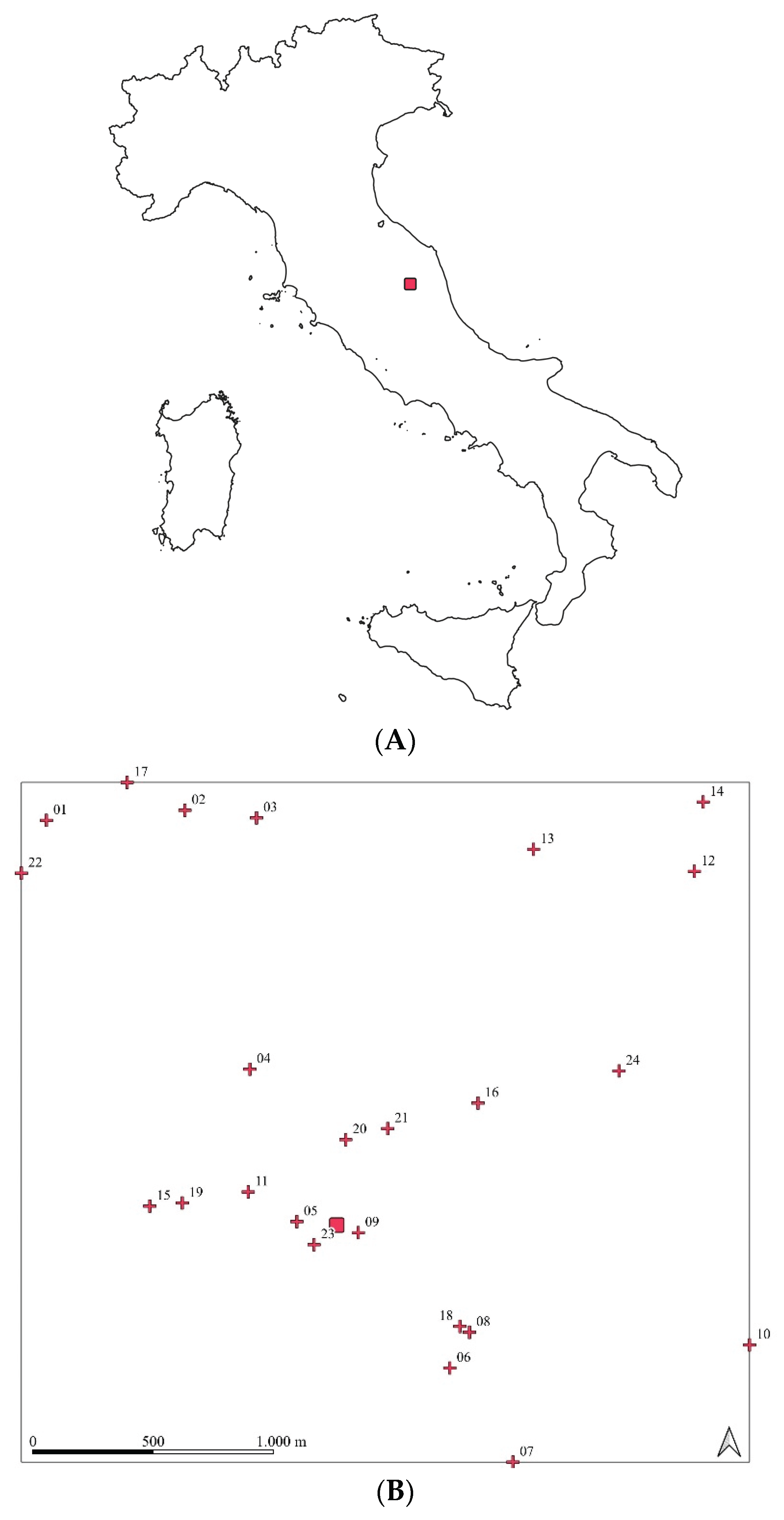
Figure 2.
Extent of spatial dataset: triangle, Farukka VHF fixes; circle, Hermione VHF fixes; red square: capture site.
Figure 2.
Extent of spatial dataset: triangle, Farukka VHF fixes; circle, Hermione VHF fixes; red square: capture site.
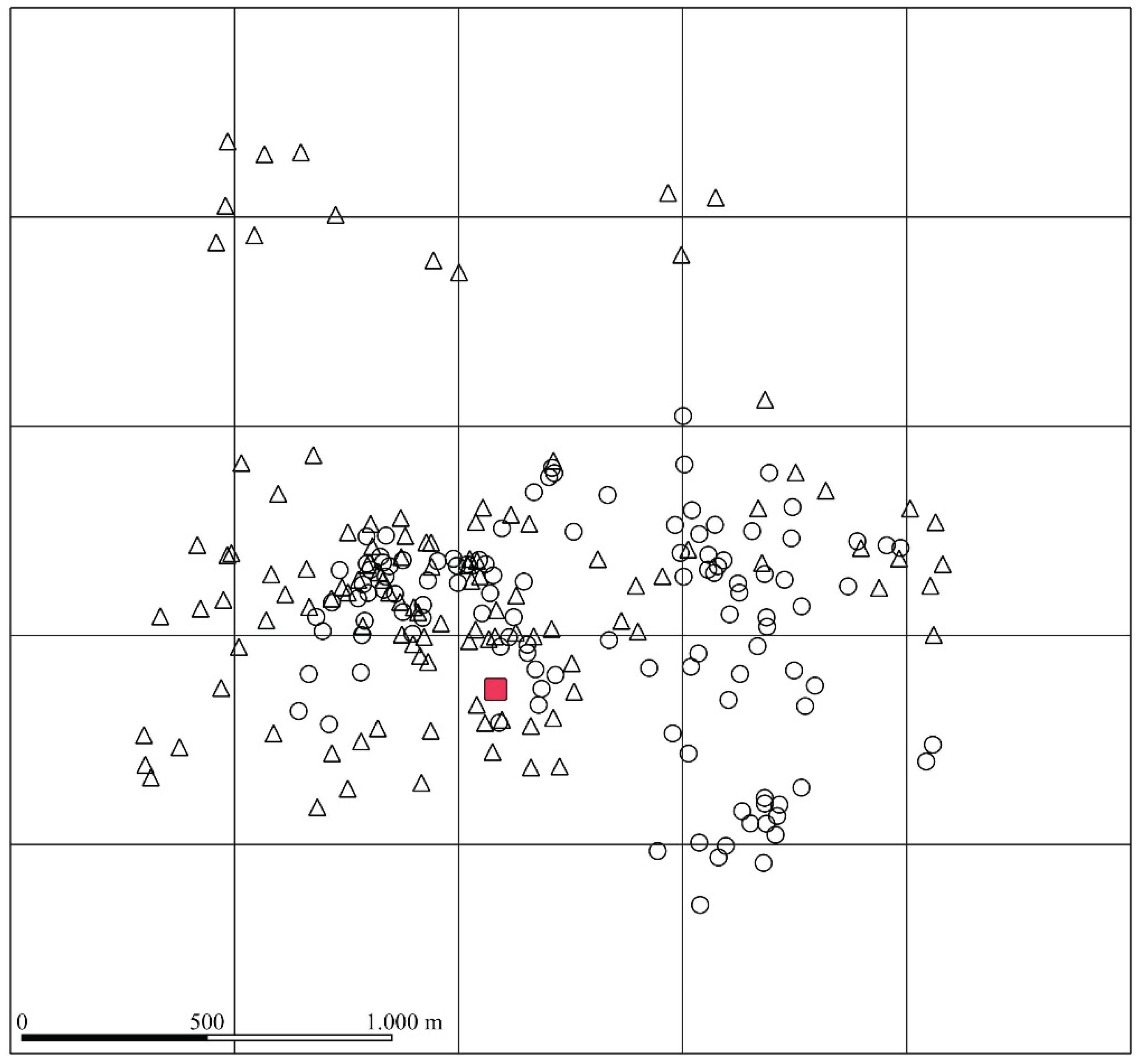
Figure 3.
Computation of home range size for various choices of the number of extreme locations to be excluded. With minimum values of up to 70% of the locations, the two females have the same home range size.
Figure 3.
Computation of home range size for various choices of the number of extreme locations to be excluded. With minimum values of up to 70% of the locations, the two females have the same home range size.
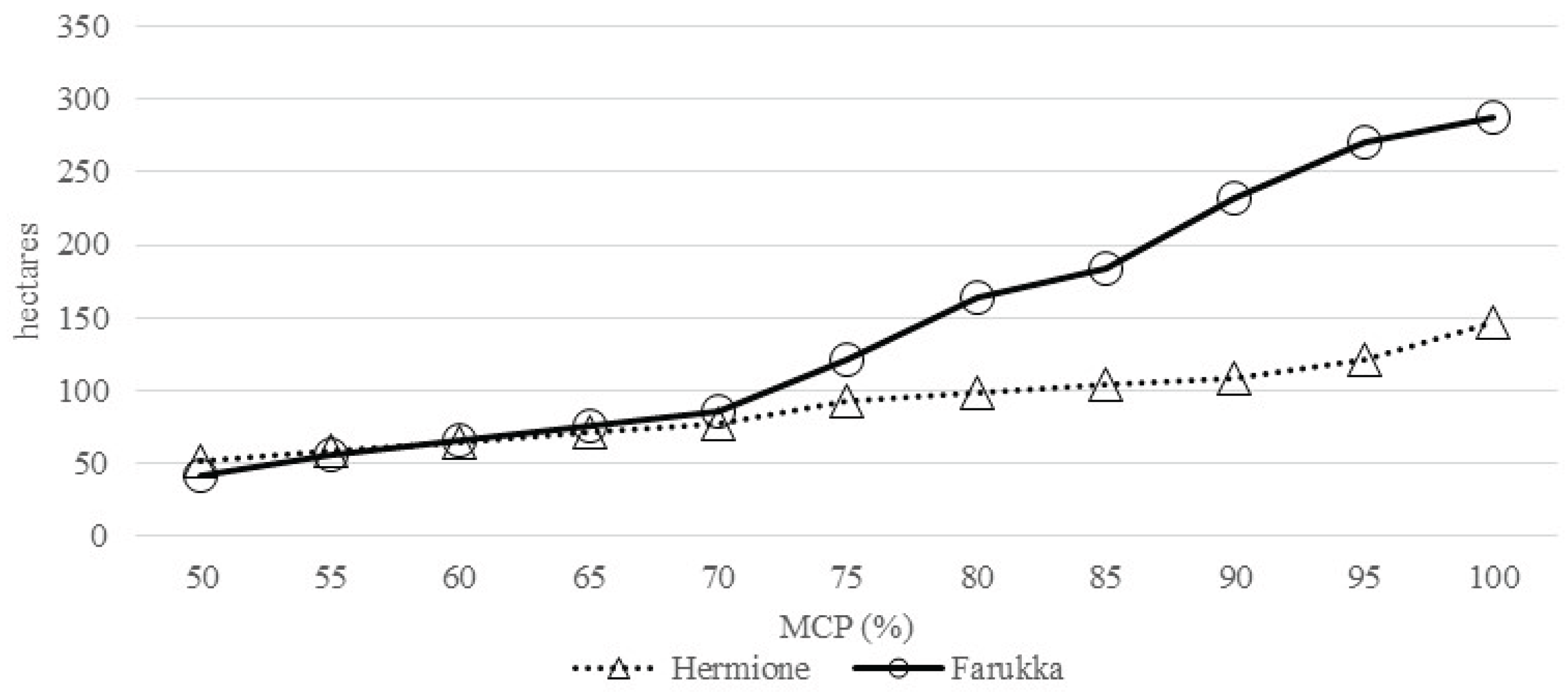
Figure 4.
Home range (MCP100) overlapping for the two wild boar females; wooded areas in grey; hydrographic network in blue; Hermione (triangle), Farukka (circle); before births (A), births (B) and after births (C).
Figure 4.
Home range (MCP100) overlapping for the two wild boar females; wooded areas in grey; hydrographic network in blue; Hermione (triangle), Farukka (circle); before births (A), births (B) and after births (C).
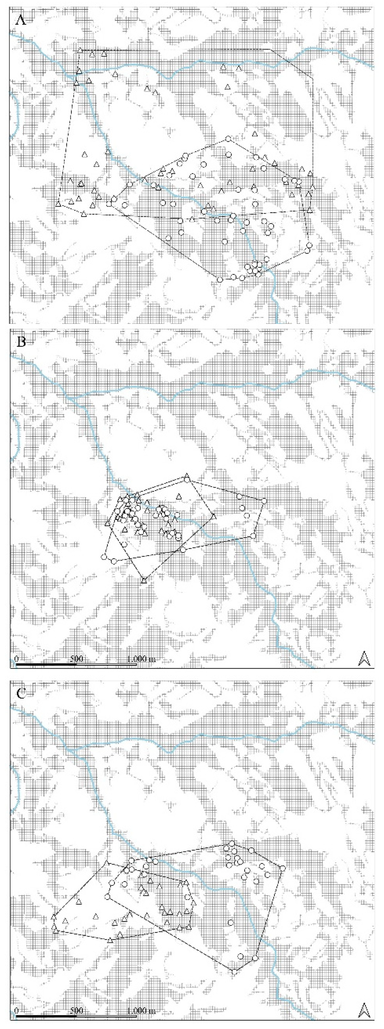

Table 1.
Summary of study area land cover.
| Landcover | Dominant Plant Species | COD | Ha | % | |
|---|---|---|---|---|---|
| Blackthorn Shrubland | Prunus spinosa | Shrub_Bl | 25,8 | 3,0 | |
| Broom Shrubland | Spartium junceum | Shrub_Br | 28,4 | 3,3 | |
| Cropland | Triticum sp.pl., Hordeum sp.pl., Helianthus annus | Crops | 261,9 | 30,6 | |
| Walnut | Juglans regia | Walnut | 2,6 | 0,3 | |
| Permanent meadows | Medicago sativa, Onobrychis vicifolia | P_mead | 69,1 | 8,1 | |
| Grassland | Bromopsis erecta, Brachypodium rupestre | Past | 42,2 | 4,9 | |
| Pre_wood vegetation | Quercus sp.pl., Ostrya carpinifolia, Acer campestre | P_wood | 48,5 | 5,7 | |
| Riverside vegetation | Quercus sp.pl., Acer campestre, Fraxinus ornus | Rv | 77,5 | 9,0 | |
| Hornbeam Forest | Ostrya carpinifolia, Quercus pubescens | Horn_forest | 280,1 | 32,7 | |
| Pinus nigra reforestation | Pinus nigra | Pinus | 9,9 | 1,2 | |
| Urban settlement | Urban | 10,4 | 1,2 | ||
| 856,4 | |||||
Table 2.
Dispersal distances (meters) from capture site. N, number of locations; SD, Standard Deviation.
Table 2.
Dispersal distances (meters) from capture site. N, number of locations; SD, Standard Deviation.
| VHF nickname | N | Mean | SD | Min | Max |
|---|---|---|---|---|---|
| Farukka | 115 | 622,68 | 399,28 | 65,91 | 1.648,89 |
| Hermione | 115 | 574,25 | 252,30 | 90,94 | 1.191,64 |
Table 3.
Home range values (hectares) measured using the minimum polygon convex (MCP) method at various percentile levels. The two females show significant difference in spatial behaviour across three distinct periods.
Table 3.
Home range values (hectares) measured using the minimum polygon convex (MCP) method at various percentile levels. The two females show significant difference in spatial behaviour across three distinct periods.
| MCP% | Hermione | Farukka | ||||
|---|---|---|---|---|---|---|
| pre-birth | birth | post-birth | pre-birth | birth | post-birth | |
| 50 | 49.7 | 7.3 | 32.1 | 125.5 | 6.3 | 13.3 |
| 55 | 59.2 | 8.2 | 33.0 | 140.5 | 6.7 | 17.6 |
| 60 | 63.2 | 9.1 | 35.7 | 153.3 | 7.8 | 20.4 |
| 65 | 68.2 | 11.0 | 37.4 | 160.9 | 8.8 | 22.8 |
| 70 | 70.0 | 11.3 | 40.2 | 174.8 | 8.8 | 26.8 |
| 75 | 75.0 | 15.9 | 41.6 | 185.1 | 9.6 | 34.3 |
| 80 | 81.5 | 24.8 | 46.4 | 202.2 | 10.4 | 36.9 |
| 85 | 88.0 | 30.0 | 51.7 | 208.0 | 10.7 | 37.9 |
| 90 | 105.1 | 44.6 | 74.2 | 219.6 | 14.4 | 46.2 |
| 95 | 112.6 | 49.7 | 78.9 | 250.5 | 19.6 | 49.2 |
| 100 | 121.6 | 58.7 | 95.5 | 275.0 | 42.1 | 51.7 |
Table 4.
Resource niche breadth (Levin’s index) for Farukka and Hermione, resource niche overlapping (Pianka’s index) and affinity between the two distributions (Bhattacharyya’s index), across three different temporal phases: pre-birth, birth and post-birth.
Table 4.
Resource niche breadth (Levin’s index) for Farukka and Hermione, resource niche overlapping (Pianka’s index) and affinity between the two distributions (Bhattacharyya’s index), across three different temporal phases: pre-birth, birth and post-birth.
| . | Levin’s index | Pianka’s index | Bhattacharyya’s index | |
|---|---|---|---|---|
| Hermione | Farukka | |||
| Pre-birth | 0.15 | 0.17 | 0.87 | 0.51 |
| Birth | 0.11 | 0.12 | 0.58 | 0.91 |
| Post-birth | 0.18 | 0.13 | 0.52 | 0.81 |
Table 5.
Environmental parameters of Farukka by phenological phases. SD, Standard deviation; pj,s, statistic differences between before births and births phase; ps,a, statistic differences between births and after births phases.
Table 5.
Environmental parameters of Farukka by phenological phases. SD, Standard deviation; pj,s, statistic differences between before births and births phase; ps,a, statistic differences between births and after births phases.
| Parameters | Before births | Births | pj,s | After births | ps,a |
|---|---|---|---|---|---|
| mean ± SD | mean ± SD | mean ± SD | |||
| Shrub_Br | 9.5 ± 3.8 | - | < 0.05 | - | - |
| Shrub_Bl | 2.4 ± 1.4 | 4.4 ± 1.1 | < 0.05 | 1.0 ± 0.6 | < 0.05 |
| Horn_forest | 30.1 ± 4.8 | 44.0 ± 6.5 | - | 48.8 ± 7.4 | - |
| Crops | 33.5 ± 4.5 | 13.9 ± 3.5 | < 0.01 | 12.9 ± 4.9 | - |
| P_wood | 0.7 ± 0.4 | 0.1 ± 0.1 | - | 9.1 ± 3.9 | < 0.05 |
| Walnut | 0.5 ± 0.5 | - | - | 0.6 ± 0.5 | - |
| Past | 0.8 ± 0.5 | 0.3 ± 0.1 | .- | - | < 0.05 |
| P_mead | 10.8 ± 4.2 | 1.2 ± 0.8 | - | 22.4 ± 5.4 | < 0.001 |
| Pinus | - | - | - | 0.4 ± 0.3 | - |
| Urban | 0.1 ± 0.1 | - | - | - | - |
| Rv | 11.9 ± 4.1 | 36.3 ± 7.2 | < 0.001 | 4.8 ± 2.3 | < 0.001 |
Table 6.
Environmental parameters of Hermione by phenological phases. SD, Standard deviation; pj,s, statistic differences between before births and births phase; ps,a, statistic differences between births and after births phases.
Table 6.
Environmental parameters of Hermione by phenological phases. SD, Standard deviation; pj,s, statistic differences between before births and births phase; ps,a, statistic differences between births and after births phases.
| Parameters | Before births | Births | pj,s | After births | ps,a |
|---|---|---|---|---|---|
| mean ± SD | mean ± SD | mean ± SD | |||
| Shrub_Br | 6.1 ± 3.4 | - | < 0.001 | 25.5 ± 7.1 | < 0.01 |
| Shurb_Bl | 3.8 ± 1.4 | 3.2 ± 1.1 | < 0.01 | 1.8 ± 0.8 | < 0.01 |
| Horn_forest | 37.5 ± 5.0 | 46.7 ± 6.6 | < 0.05 | 19.9 ± 5.8 | < 0.01 |
| Crops | 18.6 ± 3.2 | 12.6 ± 3.0 | < 0.001 | 21.4 ± 4.6 | < 0.001 |
| P_wood | 0.2 ± 0.2 | 0.1 ± 0.1 | - | - | < 0.01 |
| Walnut | 0.3 ± 0.3 | 0.1 ± 0.1 | < 0.01 | 0.3 ± 0.3 | < 0.05 |
| Past | 5.7 ± 1.9 | 2.0 ± 1.1 | < 0.001 | 3.3 ± 1.6 | < 0.05 |
| P_mead | 0.2 ± 0.2 | 0.5 ± 0.5 | - | - | - |
| Pinus | 0.1 ± 0.1 | 0.1 ± 0.1 | - | 0.4 ± 0.3 | - |
| Urban | 0.1 ± 0.1 | - | - | 0.5 ± 0.4 | - |
| Rv | 27.4 ± 2.1 | 34.8 ± 7.7 | - | 26.8 ± 5.9 | - |
Table 7.
Jacobs’ index for Farukka habitat selection according to the three phenological periods. p= proportion of habitat available in the study area; r= proportion of the habitat used by animal (e.g. % home range occupied by habitat); D= Jacobs’s index; i= indifferent; s= selected; ss= strongly selected; a= avoided; sa= strongly avoided.
| Parameter | Pre-birth | Birth | Post-birth | |||||||
|---|---|---|---|---|---|---|---|---|---|---|
| p | r | D | r | D | r | D | ||||
| Shrub_Br | 0.034 | 0.0925 | 0.4867 | i | 0.0000 | -1.0000 | sa | 0.0000 | -1.0000 | sa |
| Shurb_Bl | 0.033 | 0.0240 | -0.1620 | i | 0.0437 | 0.1454 | i | 0.0097 | -0.5530 | a |
| Horn_forest | 0.303 | 0.3009 | -0.0051 | i | 0.4397 | 0.2870 | i | 0.4878 | 0.3733 | i |
| Crops | 0.316 | 0.3349 | 0.0430 | i | 0.1386 | -0.4835 | i | 0.1291 | -0.5142 | a |
| P_wood | 0.058 | 0.0073 | -0.7860 | sa | 0.0009 | -0.9701 | sa | 0.0913 | 0.2400 | i |
| Walnut | 0.003 | 0.0047 | 0.2218 | i | 0.0000 | -1.0000 | sa | 0.0057 | 0.3078 | i |
| Past | 0.051 | 0.0083 | -0.7317 | a | 0.0026 | -0.9076 | sa | 0.0000 | -1.0000 | sa |
| P_mead | 0.083 | 0.1075 | 0.1421 | i | 0.0117 | -0.7689 | sa | 0.2244 | 0.5235 | s |
| Pinus | 0.012 | 0.0000 | -1.0000 | sa | 0.0000 | -1.0000 | sa | 0.0038 | -0.5259 | a |
| Urban | 0.013 | 0.0008 | -0.8801 | sa | 0.0000 | -1.0000 | sa | 0.0000 | -1.0000 | sa |
| Rv | 0.094 | 0.0008 | -0.9839 | sa | 0.3628 | 0.6918 | s | 0.0482 | -0.3440 | i |
Table 8.
Jacobs’ index for Hermione habitat selection according to the three phenological periods. p= proportion of habitat available in the study area; r= proportion of the habitat used by animal (e.g. % home range occupied by habitat); D= Jacobs’s index; i= indifferent; s= selected; ss= strongly selected; a= avoided; sa= strongly avoided.
| Parameter | Before births | Births | After births | |||||||
|---|---|---|---|---|---|---|---|---|---|---|
| p | r | D | r | D | r | D | ||||
| Shrub_Br | 0.034 | 0,0611 | 0,2978 | i | 0,0000 | -1,0000 | sa | 0,2552 | 0,8137 | ss |
| Shurb_Bl | 0.033 | 0,0386 | 0,0806 | i | 0,0318 | -0,0184 | i | 0,2552 | 0,8188 | ss |
| Horn_forest | 0.303 | 0,3752 | 0,1601 | i | 0,4667 | 0,3362 | i | 0,1991 | -0,2724 | i |
| Crops | 0.316 | 0,1862 | -0,3376 | i | 0,1261 | -0,5239 | a | 0,2137 | -0,2593 | i |
| P_wood | 0.058 | 0,0002 | -0,9929 | sa | 0,0011 | -0,9649 | sa | 0,0000 | -1,0000 | sa |
| Walnut | 0.003 | 0,0033 | 0,0407 | i | 0,0007 | -0,6349 | a | 0,0031 | 0,0109 | i |
| Past | 0.051 | 0,0572 | 0,0606 | i | 0,0201 | -0,4483 | i | 0,0335 | -0,2162 | i |
| P_mead | 0.083 | 0,0019 | -0,9585 | sa | 0,0046 | -0,9026 | sa | 0,0000 | -1,0000 | sa |
| Pinus | 0.012 | 0,0085 | -0,1710 | i | 0,0006 | -0,9024 | sa | 0,0037 | -0,5358 | a |
| Urban | 0.013 | 0,0006 | -0,9144 | sa | 0,0000 | -1,0000 | sa | 0,0050 | -0,4439 | i |
| Rv | 0.094 | 0,0006 | -0,9887 | sa | 0,3483 | 0,6748 | s | 0,2684 | 0,5590 | s |
Disclaimer/Publisher’s Note: The statements, opinions and data contained in all publications are solely those of the individual author(s) and contributor(s) and not of MDPI and/or the editor(s). MDPI and/or the editor(s) disclaim responsibility for any injury to people or property resulting from any ideas, methods, instructions or products referred to in the content. |
© 2025 by the authors. Licensee MDPI, Basel, Switzerland. This article is an open access article distributed under the terms and conditions of the Creative Commons Attribution (CC BY) license (http://creativecommons.org/licenses/by/4.0/).
Copyright: This open access article is published under a Creative Commons CC BY 4.0 license, which permit the free download, distribution, and reuse, provided that the author and preprint are cited in any reuse.


