
Submitted:
09 October 2025
Posted:
10 October 2025
You are already at the latest version
Abstract
The purpose of this article is to explain the introduction of simple and adaptive expo-nential smoothing methods in Life Cycle Cycle Assessment (LCA) and their results. In this case, on a cellulose factory wood debarking and cutting line. Based on a case study in which various life cycle models were applied to this asset, the application of expo-nential smoothing methods to forecast operating and maintenance costs for the t+1 pe-riod was explained; therefore, the period subsequent to the known values. The aim was to include a well-established mathematical tool in the calculation of this value, as it gives the equipment manager an idea of what is coming in the near future. Given that all forecasts end up having a Root Mean Square Error (RSME) associated with them, taking into account the actual value obtained in the previous period, this tool ends up being self-correcting and is expected to minimize the absolute error over time and as the sample size increases. Five different exponential smoothing models were applied: one simple exponential smoothing and four with adaptive parameters. As expected, it was observed that there were different results between the various methods applied. Bear-ing in mind the sample used, “Exponential smoothing with adaptive alpha 2” was the method that presented the smallest error in its forecasts, when compared to the actual values. Regardless of this specific result, the aim is for these models to be applied throughout the entire life of the asset, as well as to several different assets. So that even more detailed conclusions can be drawn about the behavior of the models in different contexts. Life cycle models are becoming increasingly reliable. With the application of robust tools to fill previously unresolved gaps, any manager and/or engineer in any field, who knows and can interpret the data collected from the asset for which they are responsible, will be able to obtain excellent results in its management. Optimizing its useful life and maximizing its availability.
Keywords:
life cycle analysis
; exponential smoothing
; physical asset management
; forecasting
; econometric models
1. Introduction
Businesses often experience the necessity to establish patterns and anticipate future costs, having also in consideration the other market variables, like interest rate, inflation, among others. Therefore, this article aims not only to assist in this task, but also proposes a tool for defining operational objectives for the business and for the assets in particular, taking into account its cost history and the market variables.
Falcão et al. (2024) agree that the use of prediction algorithms is becoming increasingly important with industrialisation. In fact, the need for prediction extends across various areas, ranging from equipment failure to anticipating future costs. Chang et al. (2024) focus their study not only on predicting customer churn, but also on the reasons behind it, since all these factors represent costs or profits for organisations.
To predict future failures based on the operating history of the asset in question, simple and adaptive exponential smoothing methods were then applied to predict the value of maintenance and operating costs in the period following the last known period, thus t+1.
In this way, the selected method is intended to be permanently updated and consolidated as the data collected increases.
Engineering Asset Management (EAM) as a discipline addresses the value contribution of AM to an organization’s success. The EAM system can be roughly defined as: “The system that plans and controls the asset-related activities and their relationships to ensure the asset performance that meets the intended competitive strategy of the organization”. This system has significant potential to influence all aspects of asset’s life cycle activities from concept design to disposal. The AM activities focus on controlling the life cycle activities of assets, but their nature is both interdisciplinary and collaborative (Amadi-Echendu et al., 2010; El-Akruti et al., 2013).
In the field of physical asset life cycles models, the progress made in recent years has been remarkable. As well as constantly evolving calculation methodologies, there has also been an evolution in the accuracy of terminology in the subject. Various authors have used terms such as Life Cycle Cost (LCC), Life Cycle Assessment (LCA) or Life Cycle Cost Analysis (LCCA), among others.
Farinha et al. (2023) claim “The subject of Life Cycle Cost (LCC) has a lack of research along time. Instead of LCC it also may managed as Life Cycle Assessment (LCA). Rarely it is treated like Life Cycle Investment (LCI). The problem of Life Cycle Cost (LCC) has received very little attention along time. LCC is also known as Life Cycle Assessment (LCA), or more rarely it is called Life Cycle Investment (LCI). By consequence, the perspectives and activity sectors from which the Physical Assets are seen may provide a specific approach”.
According to Pais et al. (2020), “Life-cycle costing shall to the extent relevant cover parts or all of the following costs over the life cycle of a product, service or works:
- a)
-
costs, borne by the contracting authority or other users, such as:
- costs relating to acquisition;
- costs of use, such as consumption of energy and other resources;
- maintenance costs;
- end of life costs, such as collection and recycling costs.
- b)
- costs imputed to environmental externalities linked to the product, service or works during its life cycle, provided their monetary value can be determined and verified; such costs may include the cost of emissions of greenhouse gases and of other pollutant emissions and other climate change mitigation costs.”
However, for maintenance and production values, it is often necessary to rely on predictions. This article discusses some exponential smoothing methods. These include simple exponential smoothing and exponential smoothing with adaptive alpha.
Farinha (2024) explains: “Based on moving average, it appears that Exponential Smoothing (ES) is a technique for smoothing time series data using the exponential window function. Whereas in the simple moving average, the past observations are weighted equally, exponential functions are used to assign exponentially decreasing weights over time. ES is a time series forecasting method for univariate data that can be extended to support data with a systematic trend or seasonal component”.
Gardner (1985) says that “the most important reason for the popularity of exponential smoothing is the surprising accuracy that can be obtained with minimal effort in model identification”. The author attempted to provide the first “comprehensive review” of the research carried out since the original work by Brown and Holt in the 1950s (Brown, 1959, 2004; Holt, 1960).
Following on from the paper, the author mentions simple exponential smoothing: “Although the simple smoothing model is a weighted moving average, it is possible to derive a smoothing parameter which gives approximately the same forecasts as an unweighted moving average of any given number of periods”. And the author goes on: “This relationship has led some researchers to conclude that simple smoothing has no important advantage in accuracy (Adam Jr (1973), with corrections by McLeavey et al. (1981); Armstrong (1978); Elton & Gruber (1972); Kirby (1966)). However, Makridakis et al., (1982) found that simple smoothing was significantly more accurate than the unweighted moving average in a sample of 1001 time series” (Gardner, 1985).
“The forecasting function is an essential element of most decision-making processes, with particular importance for management systems for planning and controlling the operations of an organization” states Ekern (1981) and adds: “Fundamentally simple forecasting methods are more widely used and accepted than are more sophisticated procedures purporting to possess desirable statistical features. Fildes (1979) ES is one such forecasting scheme which is intuitively appealing, easy to use, computationally efficient, and yet provides surprisingly accurate forecasts. (Makridakis & Hibon, 1979)”.
The author considers that, despite the robustness of simple exponential smoothing, when non-stationary data histories are found, with discontinuities, among others, it can be difficult to reach a conclusion with simple ES. So, in order to offset these difficulties, the author confirms that adaptive ES procedures replace the smoothing constant α with a smoothing parameter αt. The cellulose factory relies on wood pulp, which can vary in quality, moisture content, and fiber composition depending on supplier, region, and time of year. These fluctuations introduce non-linearities and noise into production data, making traditional forecasting methods less reliable. Exponential smoothing, especially its adaptive variants, can help filter out short-term irregularities while capturing underlying trends.
Abdelati & Hilal, (2024) states that “Simple Exponential Smoothing is the most commonly used approach due to its simplicity and effectiveness in handling data that does not trend or season”. In this study, the author also employs the exponential smoothing technique along with the calculation of the Mean Squared Error in order to improve supply chain management in the transport and automotive sectors, thereby achieving substantial improvements over existing techniques.
Monfared et al. (2014) uses an adaptive exponential smoothing method called the Revised Simple Exponential Smoothing, which proposes an alternative method for recognising non-stationary level changes in the time series. The authors find that this method improves the accuracy of the forecasting process. Through examples, results show that the mean square error can be reduced from 3.02 with Simple Exponential Smoothing to 1.34 with the new method, i.e., 2.25 times lower.
Farinha (2018) mentions “When there is a tendency to climb or fall, the second-order exponential smoothing method should be used”. The author goes on to explain: The second-order exponential smoothing method corresponds to what can be called double smoothing. Formally, it is the previous model, with the difference that the second order is applied to the prediction obtained by the exponential smoothing method (first order).
The advantage of the second-order exponential smoothing method from the previous one is that the difference between the actual value and that of the first-order forecast is approximately equal to the difference between the last and the prediction of the second order. In this way, the error between the forecast of the first order and the actual value can be corrected. This forecast provides a third estimate that, when some stability and tendencies occur, is closer to the actual value”. The cellulose production process is highly sensitive to fluctuations in the quality and characteristics of incoming biomass (e.g., wood chips, pulp). These variations affect process efficiency, energy consumption, and output consistency. Exponential smoothing helps manage this uncertainty by filtering short-term noise and identifying stable trends in input quality and production metrics.
Dielman (2006) claims that “When using exponential smoothing methods to forecast a time series, a smoothing parameter (or parameters) must be chosen. One way this choice can be made is to choose the parameter or parameters that minimize some error criterion over the history of the data available”.
In an analysis of the performance of the various forecasting methods, Ekern (1981) points out that: “For simplicity, in the subsequent re-examination the accuracy measures are the ones found in the original studies: Root Mean Squared Error (RMSE), Mean Error (ME) and Mean Absolute Deviation (MAD)”.
Raposo et al. (2017) carried out an oil analysis of a fleet of 10 buses in order to understand the importance of maintenance and determine the size of the reserve fleet. The authors took into account the reference limits proposed by the laboratories' technical data sheets in order to set values. The aim was to estimate the average value of soot and iron content. “The analysis was complemented with an analysis of the evolution of the degradation of the variables, using the Exponential Smoothing formula to predict their next values”.
Raposo et al. (2019a) and Raposo et al. (2019b) also used exponential smoothing techniques to predict future oil degradation values in order to prepare in advance for the next intervention, as part of condition monitoring based maintenance. Wiladibrata et al. (2022), on the other hand, applied exponential smoothing methods to predict the production of the Toyota Avanza in May 2022.
Dhamodharavadhani et al. (2019) have made use of exponential smoothing methods to forecast rainfall at state and district level. The authors used 3 types of exponential smoothing:
- Simple Exponential Smoothing (SES)
“The Simple Exponential Smoothing method is applied for forecasting a time series when there is no trend or seasonal pattern, but the mean (or level) of the time series yt is slowly altering over time. The present values are more weights than the past weighted averages values. This method is mostly applied for short-term forecasting that means commonly for periods not longer than 1 month (Ravinder, 2013).”
- Double Exponential Smoothing (DES)
“This method is applied when the observation data is having a trend. Double exponential smoothing method is similar to simple exponential smoothing method, but it contains two components (level and trend) that is needed for each time period. To estimate the levelled value of the observation data at the end of the period is called as level. The trend is a levelled estimate of average growth at the end of each period (Ravinder, 2013). The method is commonly known as Holt’s Linear method. It involves rapidly moving (or adjusting) the level and trend of the sequence at the end of each period. The level (Lt) is predictable by the levelled data value at the end of each period. The trend (Tt) is predictable by the levelled average increase at the end of the period. The equations for the level and trend of the series are shown in table.”
- Triple Exponential Smoothing (TES)
“Triple exponential smoothing is advanced the double exponential smoothing to model time series with seasonality. The method is also known as the Holt-Winter’s method in respects of the term of the discoverers. Holts-Winter’s method is developed by the Holt’s Linear method with adding a third parameter to deal with seasonality (Ravinder, 2013)”.
Meanwhile, Triyana Muliawati (2024) employed the exponential smoothing method to predict annual rainfall in Lampung province. By utilizing annual rainfall data from January 2010 to December 2022 (156 months) and knowing that this data has a seasonal pattern.
Aminudin et al. (2019) made use of exponential smoothing techniques in order to “forecast the Poverty Line, to help a government obtain accurate and fast information”. The authors employed the Double Exponential Smoothing Holt’s method and state that “is the right model used in poverty line forecasting where forecasting deviations are very small”, which for the application in question was below 10%.
This study aims to contribute to filling the gap in the lack of systematic research in the area of LCA, with emphasis in the time between physical asset acquisition until withdrawal, by providing the possibility of establishing goals based on an asset's operating history, using a well-established and widely studied mathematical tool. Not only that, but with the growth of historical data and with the autocorrection feature of the models, it will be possible to make short and medium term predictions that will support immediate decision-making by asset managers.
2. Methods
The research into the state of the art for this article was divided in three stages. First of all, a quick background of what is being done in the area of physical asset management and, more specifically, in the area of life cycle analysis. This ranged from review articles to more fundamental papers and books, as well as research with practical applications.
Following on from the well-known mathematical basis of the theory behind exponential smoothing methods, an effort was made to find reviews that succinctly addressed the topic. As a result, current applications of these methods in the world of engineering were presented. Focussing on studies in various areas, demonstrating the versatility of such models. It was noted that the application of this type of methodology in predicting the exploration costs of physical assets is still an area with a lot of scope for research.
Throughout the study, papers published in Q1 or Q2 journals were prioritised, although some very relevant works published in other journals were also taken into consideration.
Table 1. shows the classification of the documents used in this paper.
Together with cellulose factory, it was decided to study the life cycle of the Wood Debarking and Chipping Line acquired by the company in 2017.
This major asset consists of debarking and chipping wood so that it can later be transformed into pulp. It is therefore a critical system and extremely important for the company's operations. Upstream, the system is divided into two lines, the west line and the east line, which are responsible for debarking the wood. Downstream, these lines converge into a single one, to cut the wood and turn it into chips. The company uses both market and domestically sourced wood, which leads to variations in the market and in the cost of raw materials over time, depending on the socio-economic context and international geopolitics. Furthermore, in the case of wood, the scourge of fires directly affects its price. As such, these data are non-stationary, so the exponential smoothing approach is appropriate and applicable.
It was subsequently decided to start studying and applying two life cycle models: Life Cycle Investment and Life Cycle Recovery. In order to build any life cycle model, it is necessary to take into account some initial considerations. Therefore, both the acquisition cost (CA), the disposal value (VCn), the useful life corresponding to the disposal value (N), the Availability (A) and the operating costs (operation and maintenance) were provided by the company, as can be seen in Table 2 and Table 3.
The characters ‘k’ and ‘M’ that are added after the numbers in some of this article's tables refer to 1000 = 1k and 1000000 = 1M respectively.
As can be verified in Table 2, to prove the applicability of all the above-mentioned models, the transfer value considered was 1.00 €. Since there is no remaining value to consider, considering the cost of removing all the infrastructures.
As the variation in values from year to year is considerable, some algorithms were considered, such as simple exponential smoothing, exponential smoothing with adaptive alpha and the trend line. For these methods, the values for year 0 were excluded since it does not account for an entire period. In addition, the value for the seventh year was also ignored for the determination of the algorithm since it only contains values from the first quarter of 2024 (Equation 1).
Where,
Forecast for the next period;
Actual value recorded in the current period;
Forecast value for the current period;
Parameter smoothing;
Period.
An initial alpha of 0.3 was used for simple exponential smoothing. Equation 1 corresponds to the methodology used for this calculation, where S corresponds to the predicted value for period t and x the actual value for period t.
Where,
RSME Root Mean Square Error;
Number of periods considered.
The first forecast is made for the second year where S2 = x1. Then, the Root Mean Square Error (RSME) was calculated using the square root of the mean of the square of the error between each prediction and its actual value, using Equation 2, where T is the number of periods considered. Finally, the Excel solve tool was used to minimise the RSME by changing the alpha. The conditions limiting alpha to values between 0 and 1 were added, as shown in Equation 3.
For the exponential smoothing methods with adaptive alpha, the same methodology was applied: to find, within each model, the calculation method that would lead to the lowest RMSE. Either by adaptive exponential smoothing of the sum of the operating costs, or by the sum of the predictions obtained by adaptive exponential smoothing. All the iterations were initiated with the variables to be modelled having a value of 0.3 and then solved using Excel solver.
In the first exponential smoothing with adaptive alpha, Equations 2, 4-10 were used.
Where,
Absolute error between forecast and actual value;
Coefficient parameter smoothing;
Coefficient parameter smoothing for the previous period;
Coefficient parameter smoothing;
Coefficient parameter smoothing for the previous period;
Parameter smoothing adaptive;
Parameter smoothing adaptive.
Equations 2, 8, 9, 11 and 12 were used to construct the exponential smoothing with adaptive alpha 2.
Where,
Relative error between forecast and actual value;
Where,
Parameter smoothing adaptive for the next period;
Equations 2, 8, 9, 11 and condition 13 were used for the exponential smoothing with adaptive alpha 3
Where,
E_(t-1) Absolute error between the previous period's forecast and the respective current value;
Parameter smoothing adaptive for the previous period.
The exponential smoothing with adaptive alpha 4 consisted of equations 4, 5, 8-11, 14 and 15.
3. Results
After applying the models explained above, several tables and graphs were produced to illustrate the results that had been obtained.
3.1. Simple Exponential Smoothing
Table 4 shows the result obtained for the simple exponential smoothing of operating costs (CE).
Figure 1 shows the graph obtained with the real and estimated values, as well as the polynomial trend line of 4th degree obtained with the simple exponential smoothing of CE.
At the end, an attempt was made to realise whether the error is greater by exponentially smoothing the CE or by summing the predictions obtained through simple exponential smoothing of the CO and CM. The conclusion was that, with this exponential smoothing, the first method provides a lower RMSE, as can be seen in Table 5, Table 6 and Table 7.
3.2. Exponential Smoothing with Adaptive Alpha
The obtained results for exponential smoothing with adaptive alpha 1 of the sum of operating costs, and consequently where the smallest error lies, are shown in Table 8 and in the graph of Figure 2. The values achieved for the sum of the forecasts obtained by exponential smoothing with adaptive alpha are shown in Table 9, Table 10 and Table 11.
Table 12, Table 13, Table 14 and Table 15 were thus calculated, showing that the sum of the CO and CM forecasts achieved through the exponential smoothing with adaptive alpha 2 had the lowest RMSE value when compared to the exponential smoothing with adaptive alpha 2 of CE. Therefore, the graph shown in Figure 3 is representative of the values provided in Table 14.
4. Discussion
The use of five different exponential smoothing models, especially the four adaptive models, aims to overcome the issue of non-stationary data histories, with discontinuities, among others, which are typical in industrial environments with raw material variability and unpredictable maintenance costs. Furthermore, these are self-correcting models, so it is expected that the results will improve over time, except in the case of atypical constraints such as wars or pandemics.
Gathering the minimum RMSE values for each method, it can be state that the lowest value is obtained using the exponential smoothing with adaptive alpha 2 approach, as can be seen in Table 24 and the graph in Figure 6.
Although it seems that using the polynomial trend line of degree 4 can produce relatively decent results, it is not at all the best option for this asset, given the large difference from year to year.
However, for any of the exponential smoothing methods, predictions can only be made for the period t+1, so it is not possible to make predictions up to the period considered for the cession value.
The company did not communicate its maximum cost targets per period until the end of the asset's useful life, which would effectively be the best option for the company's management and planning area.
Table 15 shows that, compared to the other methods, exponential smoothing with adaptive alpha 2 has the lowest RMSE. In other words, the average error between the forecasts calculated and the results obtained was the lowest. This tool makes life easier for managers when there are no other possibilities for predicting future values. Despite being a tool that cuts across various sectors, it often manages to provide reliable data. This allows an estimate to be made for the following period.
In this case, the sum of the forecasts made using exponential smoothing of maintenance costs and operating costs shows less error compared to the forecast made using exponential smoothing of the sum of exploration costs, as can be seen in Table 12, Table 13 and Table 14.
Although relative errors of 29% and 43% were obtained in periods 3 and 5 respectively, much smaller deviations were obtained in periods 4 and 6, in the order of 6% and 2% each.
The time between year 3 and year 4 corresponds exactly to the period of lockdown due to the COVID-19 pandemic. This deviation directly impacts the exponential smoothing forecasts for that year, but not only. Since this is a self-correcting model, it will also impact forecasts for subsequent years until the data stabilises and normalises. It is possible to see the impact that this event had on the data and its forecasts, making it clear to justify.
As a result, it was chosen to use the values predicted by the exponential smoothing with adaptive alpha 2 method for period 8. But first it became necessary to determine the costs for the whole of year 7. The values for the first 2 months were then multiplied by 6 to obtain the value for the 12 months. Although the costs do not behave linearly over the course of a calendar year, this was considered the most appropriate approach in this case.
As a result, the following figures were obtained for the 7th period:
- • CO7 = 812 183.82 €;
- • CM7 = 1 400 612.10 €;
- • CE7 = 2 212 795.92 €.
For the 8th year of operation, the following values were found using the exponential smoothing method with adaptive alpha 2:
- • CO8 = 524 776.68 €;
- • CM8 = 1 450 746.57 €;
- • CE8 = 1 975 523.25 €.
To establish the remaining exploration cost amounts up to the 35th period, two different methods were employed. For the operating cost, a constant value was taken from calculating the average of the first 7 years of operation - 278 131.96 €. For maintenance costs, a 20 per cent increase was considered each year until the end of equipment's life.
5. Conclusions
Credible results were obtained, paving the way for the next steps in this study. In fact, there are countless tools that can be used to predict “next instants” in the field of prediction. Exponential smoothing is always a tool that adds value to this area.
This research demonstrated its applicability in a subject in which there is very little published work and, by consequence, it adds value to the state of art. It also helps the physical asset managers, because, based on this research, they can support their decision about physical assets in a new methodology applied during the life cycle of the assets.
Rather than making only predictions for next period, this research allows managers to set targets and limits relating to exploration costs in the short and medium term, based on the errors obtained and the predicted values. Focusing on these results, it makes possible to analyse the data at the end of the next period and find the causes of possible deviations from reality. These deviations can be due to uncontrollable conditions (e.g. international conflicts that influence the markets), or due to operational failures or poor planning.
Following the publication of this article, the research will proceed with a review of the models applied and the results obtained: Life Cycle Investment and Life Cycle of Physical Assets with Recovery.
A further review will then be made of hypothetical scenarios and how life cycle models can help to predict and counteract specific circumstances. Of course, they can also be used as strategic tools when setting exploration objectives.
Author Contributions
Conceptualization, P. F., H. R. and T. F.; Methodology, P. F., H. R. and T. F.; formal analysis, P. F., H. R. and T. F.; investigation, P. F.; writing—original draft preparation, P. F.; writing—review and editing, H. R. and T. F.; supervision, H. R. and T. F. All authors have read and agreed to the published version of the manuscript.
Funding
Funding provided by Research Centre in Asset Management and System Engineering (RCM2+).
Data availability statement
The data sets generated during this study are available from the corresponding author upon reasonable request.
Conflicts of interest
The authors have no relevant financial or nonfinancial interests to disclose.
References
- Abdelati, M. H., & Hilal, N. (2024). Optimizing Simple Exponential Smoothing for Time Series Forecasting in Supply Chain Management. Indonesian Journal of Innovation and Applied Sciences (IJIAS), 4(3), 247–256. [CrossRef]
- Adam Jr, E. E. (1973). Individual item forecasting model evaluation. Decis. Sci., 4(4), 458–470. [CrossRef]
- Amadi-Echendu, J. E., Willett, R., Brown, K., Hope, T., Lee, J., Mathew, J., Vyas, N., & Yang, B.-S. (2010). What Is Engineering Asset Management?
- Aminudin, R., & Putra, Y. H. (2019). Poverty Line Forecasting Model Using Double Exponential Smoothing Holt’s Method. IOP Conference Series: Materials Science and Engineering, 662(6). [CrossRef]
- Armstrong, J. S. (1978). Long-range Forecasting: From Crystal Ball to Computer. Wiley. ISBN-10: 0471822604, ISBN-13: 978-0471822608.
- Brown, R. G. (1959). Statistical Forecasting for Inventory Control. McGraw-Hill. ISBN-10: 007008145X, ISBN-13: 978-0070081451.
- Brown, R. G. (1963). Smoothing, Forecasting and Prediction of Discrete Time Series. Dover ISBN-10: 9780138153083, ISBN-13: 978-0138153083.
- Chang, V., Hall, K., Xu, Q. A., Amao, F. O., Ganatra, M. A., & Benson, V. (2024). Prediction of Customer Churn Behavior in the Telecommunication Industry Using Machine Learning Models. Algorithms, 17(6), 231–231. [CrossRef]
- Dhamodharavadhani, S., & Rathipriya, R. (2019). Region-Wise Rainfall Prediction Using MapReduce-Based Exponential Smoothing Techniques. Advances in Intelligent Systems and Computing, 750, 229–239. [CrossRef]
- Dielman, T. (2006). Choosing smoothing parameters for exponential smoothing: Minimizing sums of squared versus sums of absolute errors. J. Mod. Appl. Stat. Methods, 5, 118–129. [CrossRef]
- Ekern, S. (1981). Adaptive Exponential Smoothing Revisited (Vol. 32). [CrossRef]
- El-Akruti, K., Dwight, R., & Zhang, T. (2013). The strategic role of Engineering Asset Management. Int. J. Prod. Econ., 146(1), 227–239. [CrossRef]
- Elton, E. J., & Gruber, M. J. (1972). Earnings estimates and the accuracy of expectational data. Manag. Sci., 18(8), B-409. [CrossRef]
- Falcão, D., Reis, F., Farinha, J., Lavado, N., & Mendes, M. (2024). Fault Detection in Industrial Equipment through Analysis of Time Series Stationarity. Algorithms, 17(10), 455. [CrossRef]
- Farinha, J. M. T. (2018). Asset Maintenance Engineering Methodologies. ISBN-10: 1138035890, ISBN-13: 978-1138035898.
- Farinha, J. M. T. (2024). Physical Asset Management for a Sustainable World. ISBN: 9781032428352.
- Farinha, J. M. T., Raposo, H. N., Pais, E. A., & Mendes, M. (2023). Physical Assets Life Cycle Evaluation Models – A Comparative Analysis Aiming the Sustainability. Sustain. 2023, 15(22), 15754; [CrossRef]
- Fildes, R. (1979). Quantitative forecasting—The state of the art: Extrapolative models. J. Oper. Res. Soc., 30(8), 691–710. [CrossRef]
- Gardner, E. S. (1985). Exponential Smoothing: The State of the Art. J. Forec. (Vol. 4). [CrossRef]
- Holt, C. C. (1960). Planning Production, Inventories, and Work Force. ISBN- 10: 0136797466, ISBN-13: 978-0136797463.
- Kirby, R. M. (1966). A comparison of short and medium range statistical forecasting methods. Manag. Sci., 13(4), B-202. [CrossRef]
- Makridakis, S., Andersen, A., Carbone, R., Fildes, R., Hibon, M., Lewandowski, R., Newton, J., Parzen, E., & Winkler, R. (1982). The accuracy of extrapolation (time series) methods: Results of a forecasting competition. J. Forec., 1(2), 111–153. [CrossRef]
- Makridakis, S., & Hibon, M. (1979). Accuracy of forecasting: An empirical investigationJ. R. Stat. Soc. Ser. A (Gen.), 142(2), 97–125. [CrossRef]
- McLeavey, D. W., Lee, T. S., & Adam Jr, E. E. (1981). An empirical evaluation of individual item forecasting models. Decis. Sci., 12(4), 708–714. [CrossRef]
- Monfared, M. A. S., Ghandali, R., & Esmaeili, M. (2014). A new adaptive exponential smoothing method for non-stationary time series with level shifts. Journal of Industrial Engineering International, 10(4), 209–216. [CrossRef]
- Pais, E., Farinha, J. T., Cardoso, A. J. M., & Raposo, H. (2020). Optimizing the life cycle of physical assets – A review. WSEAS Trans. Syst. ControlControl (Vol. 15, pp. 417–430). World Scientific and Engineering Academy and Society. [CrossRef]
- Raposo, H., Farinha, J. T., Ferreira, L., & Galar, D. (2017). An integrated econometric model for bus replacement and determination of reserve fleet size based on predictive maintenance. Eksploat. Niezawodn. 19(3), 358–368. [CrossRef]
- Raposo, H., Farinha, J. T., Fonseca, I., & Ferreira, L. A. (2019b). Condition monitoring with prediction based on diesel engine oil analysis: A case study for urban buses. Actuators, 8(1). [CrossRef]
- Raposo, H., Farinha, J. T., Fonseca, I., & Galar, D. (2019a). Predicting condition based on oil analysis – A case study. Tribol. Int., 135, 65–74. [CrossRef]
- Ravinder, H. V. (2013). Determining the Optimal Values of Exponential Smoothing Constants--Does Solver Really Work?. Am. J. Bus. Educ., 6(3), 347–360. [CrossRef]
- Triyana Muliawati. (2024). Analysis of Rainfall Prediction in Lampung Province using the Exponential Smoothing Method. Int. J. Sci. Res. Sci. Eng. Technol., 232–240. [CrossRef]
- Wiladibrata, M. I., & Komara Rifai, N. A. (2022). Peramalan Produksi Mobil Menggunakan Metode Double Exponential Smoothing dengan Algoritma Golden Section. Bandung Conf. Ser. Stat., 2(2), 507–511. [CrossRef]
Figure 1.
Simple exponential smoothing of CE.
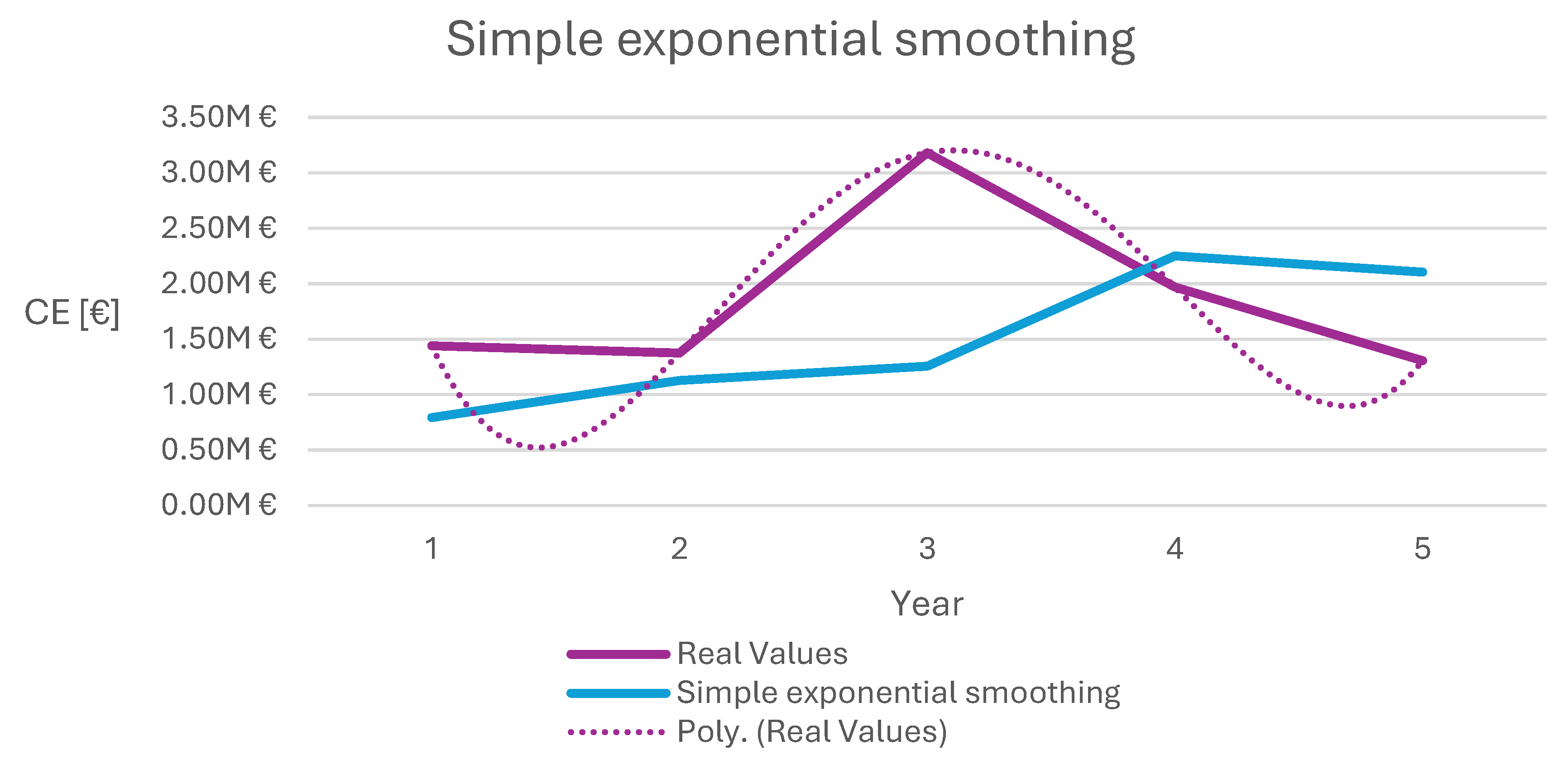
Figure 2.
Exponential smoothing with adaptive alpha 1 of CE.
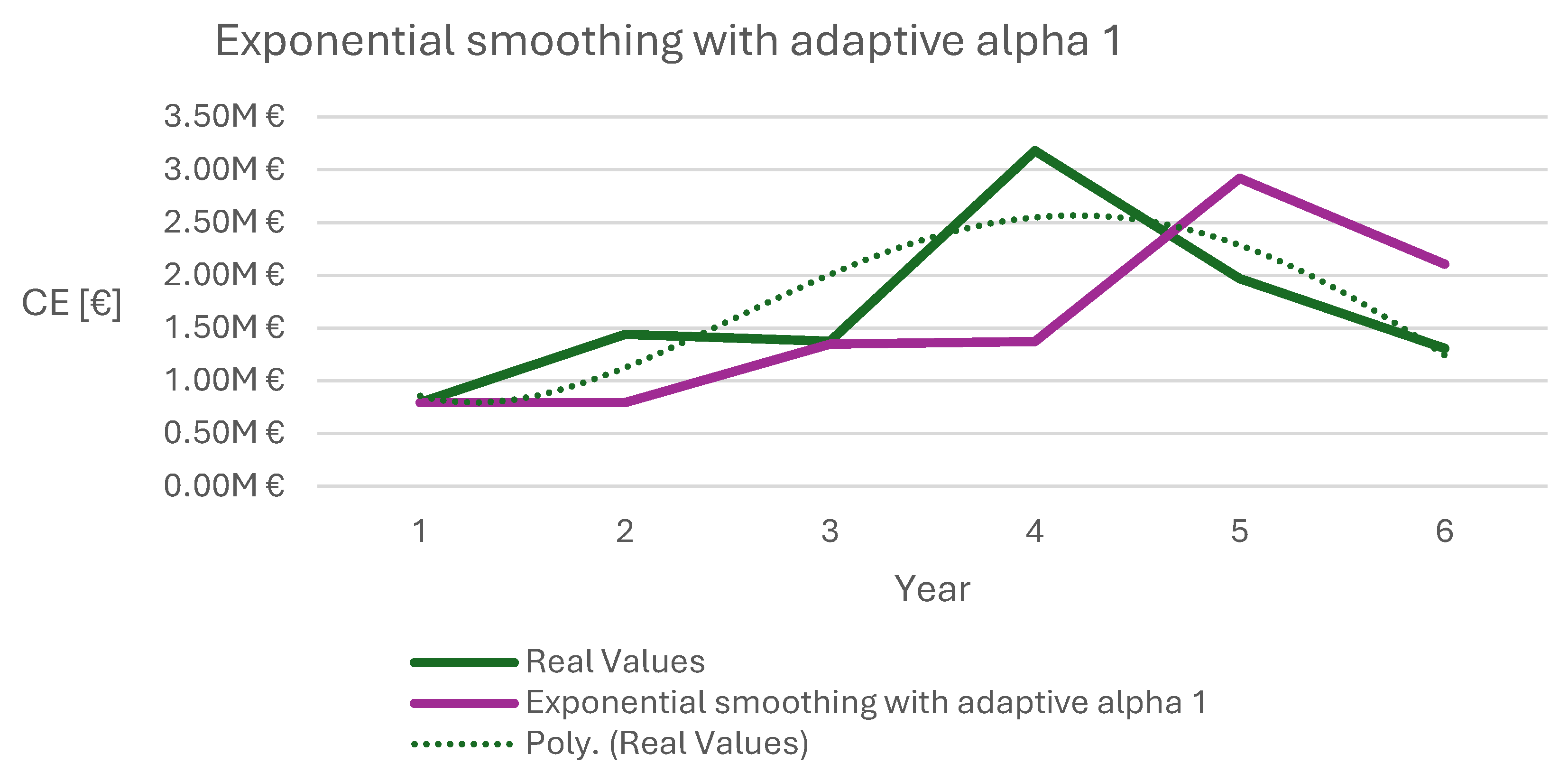
Figure 3.
Sum of exponential smoothing with adaptive alpha 2 of CO and CM.
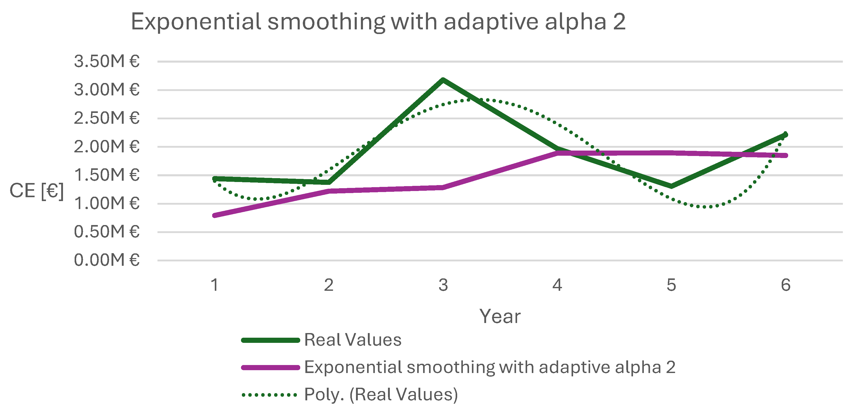
Figure 4.
Sum of exponential smoothing with adaptive alpha 3 of CO and CM.

Figure 5.
Sum of exponential smoothing with adaptive alpha 4 of CO and CM.
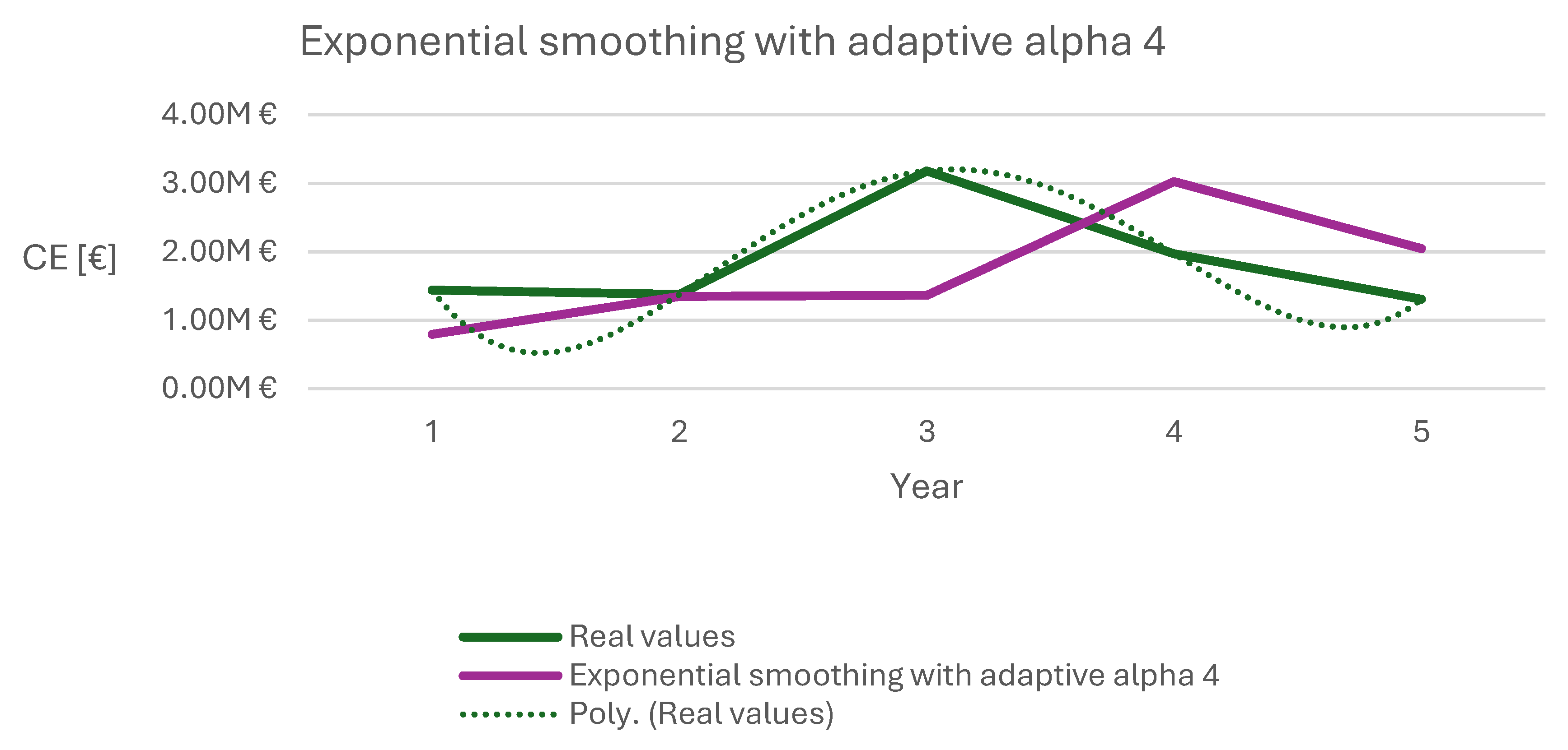
Figure 6.
All methods- Case Study.
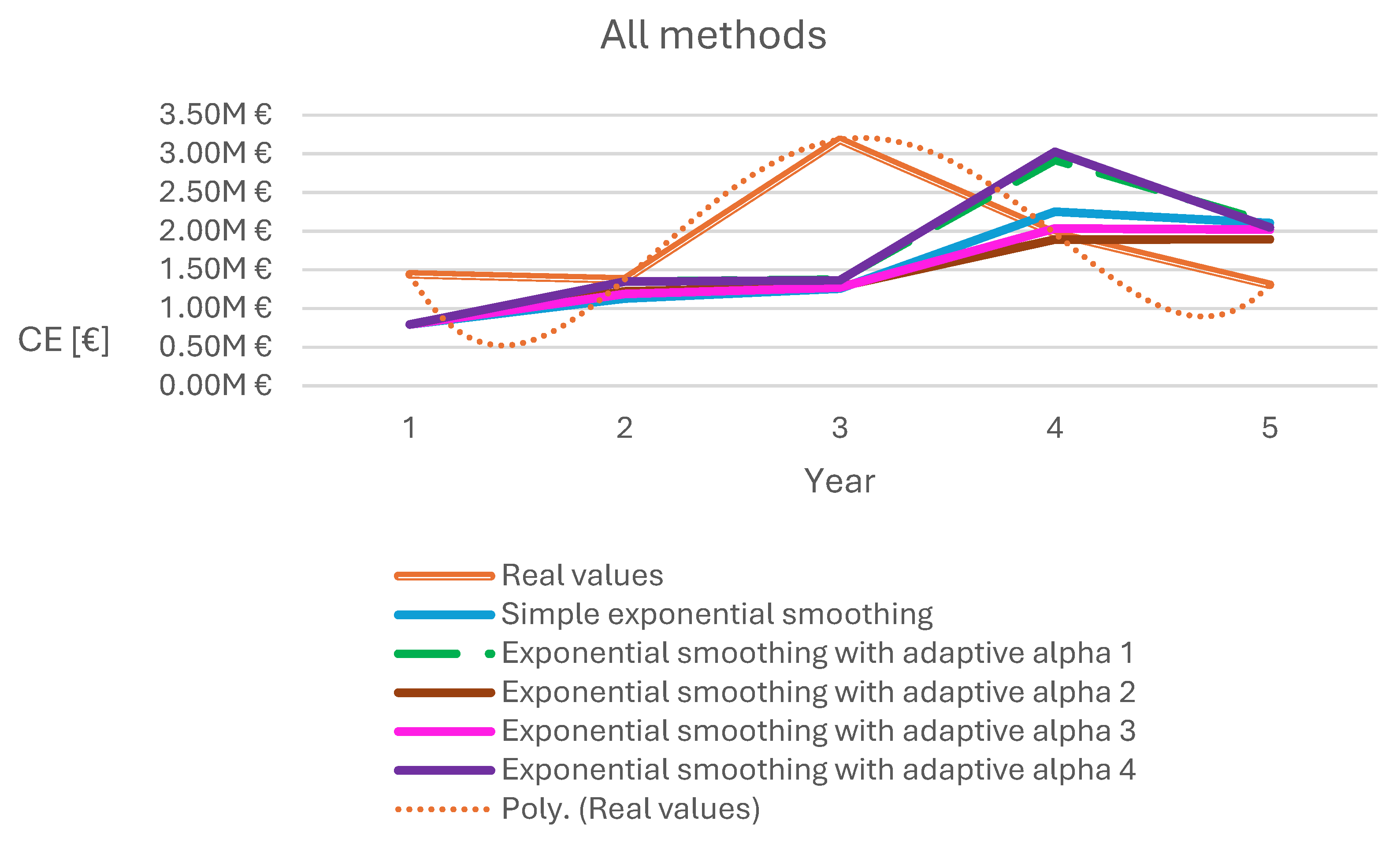

Table 1.
Classification of the papers.
| Reference Number | Author | Title | Cl. |
|---|---|---|---|
| 1 | Abdelati & Hilal | Optimizing Simple Exponential Smoothing for Time Series Forecasting in Supply Chain Management | Not indexed |
| 2 | E. E. Adam Jr. | Individual item forecasting model evaluation | Q1 |
| 3 | J. E. Amadi-Echendu et al. | What Is Engineering Asset Management? | Q4 |
| 4 | R. Aminudin et al. | Poverty Line Forecasting Model Using Double Exponential Smoothing Holt’s Method | Not indexed |
| 8 | Chang et al. | Prediction of Customer Churn Behavior in the Telecommunication Industry Using Machine Learning Models |
Q2 |
| 9 | S. Dhamodharavadhani et al. | Region-Wise Rainfall Prediction Using MapReduce-Based Exponential Smoothing Techniques | Q4 |
| 10 | T. Dielman | Choosing smoothing parameters for exponential smoothing: Minimizing sums of squared versus sums of absolute errors | Q4 |
| 11 | S. Ekern | Adaptive Exponential Smoothing Revisited | Q2 |
| 12 | K. El-Akruti et al. | The Strategic Role of Engineering Asset Management | Q1 |
| 13 | E. J. Elton et al. | Earnings estimates and the accuracy of expectational data | Q1 |
| 14 | Falcão et al. | Fault Detection in Industrial Equipment through Analysis of Time Series Stationarity | Q2 |
| 17 | Farinha, J. T. et al. | Physical Asset Life Cycle Evaluation Models—A Comparative Analysis towards Sustainability | Q1 |
| 18 | R. Fildes | Quantitative forecasting—The state of the art: Extrapolative models | Q2 |
| 19 | E. S. Gardner | Exponential smoothing: The state of the art | Q2 |
| 21 | R. M. Kirby | A comparison of short and medium range statistical forecasting methods | Q1 |
| 22 | S. Makridakis et al. | The accuracy of extrapolation (time series) methods: Results of a forecasting competition | Q2 |
| 23 | S. Makridakis et al. | Accuracy of forecasting: An empirical investigation | Q2 |
| 24 | D. W. McLeavey et al. | An empirical evaluation of individual item forecasting models | Q1 |
| 25 | Monfared et al. | A new adaptive exponential smoothing method for non-stationary time series with level shifts |
Q2 |
| 26 | Pais et al. | Optimizing the Life Cycle of Physical Assets – a Review | Q4 |
| 27 | H. Raposo et al. | An integrated econometric model for bus replacement and determination of reserve fleet size based on predictive maintenance | Q2 |
| 28 | H. Raposo et al. | Condition monitoring with prediction based on diesel engine oil analysis: A case study for urban buses | Q2 |
| 29 | H. Raposo et al. | Predicting condition based on oil analysis – A case study | Q1 |
| 30 | H. V Ravinder | Determining the Optimal Values of Exponential Smoothing Constants--Does Solver Really Work? | Not indexed |
| 31 | Triyana Muliawati | Analysis of Rainfall Prediction in Lampung Province using the Exponential Smoothing Methodechnol | Not indexed |
| 32 | M. I. Wiladibrata et al. | Peramalan Produksi Mobil Menggunakan Metode Double Exponential Smoothing dengan Algoritma Golden Section | Not indexed |
Table 2.
- Wood Debarking and Chipping Line Acquisition Data (Paper Pulp Company).
| Acquisition data | ||
|---|---|---|
| Acquisition cost | CA | 18 156 000.00 € |
| Cessation value | VCn | 1.00 € |
| Lifetime corresponding to VCn | N | 35 |
| Average Availability | A | 54% |
Table 3.
Wood Debarking and Chipping Line Annual Explotation Costs (Paper Pulp Company).
| Year | Annual operating cost | Annual maintenance cost | Annual Exploitation Cost |
|---|---|---|---|
| 0 | 78.0k € | 22.2k € | 100.2k € |
| 1 | 167.2k € | 625.7k € | 792.8k € |
| 2 | 401.8k € | 1.038M € | 1.440M € |
| 3 | 335.5k € | 1.040M € | 1.376M € |
| 4 | 716.8k € | 2.463M € | 3.180M € |
| 5 | 363.8k € | 1.605M € | 1.969M € |
| 6 | 320.3k € | 985.7k € | 1.306M € |
| 7 | 135.4k € | 233.4k € | 368.8k € |
| Total | 2.519M € | 8.014M € | 10.533M € |
Table 4.
Simple exponential smoothing of CE.
| Year | Annual Exploitation Cost | Prediction | Error2 | α |
|---|---|---|---|---|
| 1 | 792.84k € | - | - | 0.52 |
| 2 | 1.44M € | 792.84k € | 4.19E+11 | |
| 3 | 1.38M € | 1.13M € | 6.16E+10 | |
| 4 | 3.18M € | 1.26M € | 3.70E+12 | |
| 5 | 1.97M € | 2.25M € | 7.91E+10 | |
| 6 | 1.31M € | 2.10M € | 6.38E+11 | |
| Mean | 9.80E+11 | |||
| RMSE | 990 044.01 € | |||
Table 5.
Simple exponential smoothing of CO.
| Year | Annual Operation Cost | Prediction | Error2 | α |
|---|---|---|---|---|
| 1 | 167.15k € | - | - | 0.49 |
| 2 | 401.84k € | 167.15k € | 5.51E+10 | |
| 3 | 335.54k € | 281.07k € | 2.97E+09 | |
| 4 | 716.80k € | 307.51k € | 1.68E+11 | |
| 5 | 363.81k € | 506.19k € | 2.03E+10 | |
| 6 | 320.26k € | 437.08k € | 1.36E+10 | |
| Mean | 5.19E+10 | |||
| RMSE | 227 807.41 € | |||
Table 6.
Simple exponential smoothing of CM.
| Year | Annual Maintenance Cost | Prediction | Error2 | α |
|---|---|---|---|---|
| 1 | 625.68k € | - | - | 0.52 |
| 2 | 1.04M € | 625.68k € | 1.70E+11 | |
| 3 | 1.04M € | 839.33k € | 4.03E+10 | |
| 4 | 2.46M € | 943.22k € | 2.31E+12 | |
| 5 | 1.61M € | 1.73M € | 1.56E+10 | |
| 6 | 985.67k € | 1.67M € | 4.62E+11 | |
| Mean | 6.00E+11 | |||
| RMSE | 774 393.45 € | |||
Table 7.
Sum of CO and CM predictions.
| Year | Annual Exploitation Cost | Prediction | Error2 |
|---|---|---|---|
| 1 | 792.84k € | - | - |
| 2 | 1.44M € | 792.84k € | 4.19E+11 |
| 3 | 1.38M € | 1.12M € | 6.51E+10 |
| 4 | 3.18M € | 1.25M € | 3.72E+12 |
| 5 | 1.97M € | 2.24M € | 7.14E+10 |
| 6 | 1.31M € | 2.10M € | 6.34E+11 |
| Mean | 9.82E+11 | ||
| RMSE | 991 163.80 € | ||
Table 8.
Exponential smoothing with adaptive alpha 1 of CE.
| Year | Annual Exploitation Cost | Prediction | 2 | α | At | Mt | β | |
|---|---|---|---|---|---|---|---|---|
| 1 | 792.84k € | 792.84k € | - | - | 0.860 | 0.63 | 0.74 | 0.00 |
| 2 | 1.44M € | 792.84k € | 6.47E+05 | 4.19E+11 | 0.856 | 0.63 | 0.74 | |
| 3 | 1.38M € | 1.35M € | 2.87E+04 | 8.23E+08 | 0.856 | 0.63 | 0.74 | |
| 4 | 3.18M € | 1.37M € | 1.81E+06 | 3.27E+12 | 0.856 | 0.63 | 0.74 | |
| 5 | 1.97M € | 2.92M € | -9.50E+05 | 9.03E+11 | 0.856 | 0.63 | 0.74 | |
| 6 | 1.31M € | 2.11M € | -8.00E+05 | 6.40E+11 | 0.856 | 0.63 | 0.74 | |
| Mean | 1.05E+12 | |||||||
| RMSE | 1023100.957 | |||||||
Table 9.
Exponential smoothing with adaptive alpha 1 of CO.
| Year | Annual Operation Cost | Prediction | 2 | α | At | Mt | β | |
|---|---|---|---|---|---|---|---|---|
| 1 | 167.15k € | 167.15k € | - | - | 0.60 | 0.55 | 0.91 | 0.00 |
| 2 | 401.84k € | 167.15k € | 2.35E+05 | 5.51E+10 | 0.60 | 0.55 | 0.91 | |
| 3 | 335.54k € | 308.57k € | 2.70E+04 | 7.27E+08 | 0.60 | 0.55 | 0.91 | |
| 4 | 716.80k € | 324.83k € | 3.92E+05 | 1.54E+11 | 0.60 | 0.55 | 0.91 | |
| 5 | 363.81k € | 561.03k € | -1.97E+05 | 3.89E+10 | 0.60 | 0.55 | 0.91 | |
| 6 | 320.26k € | 442.18k € | -1.22E+05 | 1.49E+10 | 0.60 | 0.55 | 0.91 | |
| Mean | 5.26E+10 | |||||||
| RMSE | 229440.2771 | |||||||
Table 10.
Exponential smoothing with adaptive alpha 1 of CM.
| Year | Annual Operation Cost | Prediction | 2 | α | At | Mt | β | |
|---|---|---|---|---|---|---|---|---|
| 1 | 625.68k € | 625.68k € | - | - | 0.940 | 0.94 | 9.99E-01 | 0.00 |
| 2 | 1.04M € | 625.68k € | 4.13E+05 | 1.70E+11 | 0.939 | 0.94 | 9.99E-01 | |
| 3 | 1.04M € | 1.01M € | 2.66E+04 | 7.08E+08 | 0.939 | 0.94 | 9.99E-01 | |
| 4 | 2.46M € | 1.04M € | 1.42E+06 | 2.03E+12 | 0.939 | 0.94 | 9.99E-01 | |
| 5 | 1.61M € | 2.38M € | -7.72E+05 | 5.96E+11 | 0.939 | 0.94 | 9.99E-01 | |
| 6 | 985.67k € | 1.65M € | -6.66E+05 | 4.44E+11 | 0.939 | 0.94 | 9.99E-01 | |
| Mean | 6.48E+11 | |||||||
| RMSE | 805028.4195 | |||||||
Table 11.
Sum of CO and CM predictions with exponential smoothing with adaptive alpha 1.
| Year. | Annual Exploitation Cost | Prediction | 2 | |
|---|---|---|---|---|
| 1 | 792.84K € | 792.84k € | - | - |
| 2 | 1.44M € | 792.84k € | 6.47E+05 | 4.19E+11 |
| 3 | 1.38M € | 1.32M € | 5.36E+04 | 2.87E+09 |
| 4 | 3.18M € | 1.36M € | 1.82E+06 | 3.30E+12 |
| 5 | 1.97M € | 2.94M € | -9.69E+05 | 9.39E+11 |
| 6 | 1.31M € | 2.09M € | -7.88E+05 | 6.21E+11 |
| Mean | 1.06E+12 | |||
| RMSE | 1027864.215 | |||
Table 12.
Exponential smoothing with adaptive alpha 2 of CE.
| Year | Annual Exploitation Cost | Prediction | α | 2 | ||
|---|---|---|---|---|---|---|
| 1 | 792.84k € | 792.84k € | 0% | 0.67 | - | - |
| 2 | 1.44M € | 792.84k € | 0% | 0.67 | 6.47E+05 | 4.19E+11 |
| 3 | 1.38M € | 1.22M € | 29% | 0.67 | 1.51E+05 | 2.29E+10 |
| 4 | 3.18M € | 1.28M € | 6% | 0.38 | 1.90E+06 | 3.61E+12 |
| 5 | 1.97M € | 1.88M € | 43% | 0.32 | 8.41E+04 | 7.08E+09 |
| 6 | 1.31M € | 1.89M € | 2% | 0.11 | -5.88E+05 | 3.46E+11 |
| Mean | 8.80E+11 | |||||
| RMSE | 938146.0483 | |||||
Table 13.
Exponential smoothing with adaptive alpha 2 of CO.
| Year | Annual Operation Cost | Prediction | α | 2 | ||
|---|---|---|---|---|---|---|
| 1 | 167.15k € | 167.15k € | 0% | 0.65 | - | - |
| 2 | 401.84k € | 167.15k € | 0% | 0.65 | 2.35E+05 | 5.51E+10 |
| 3 | 335.54k € | 319.40k € | 41% | 0.65 | 1.61E+04 | 2.61E+08 |
| 4 | 716.80k € | 323.22k € | 2% | 0.24 | 3.94E+05 | 1.55E+11 |
| 5 | 363.81k € | 406.51k € | 38% | 0.21 | -4.27E+04 | 1.82E+09 |
| 6 | 320.26k € | 399.39k € | -6% | 0.17 | -7.91E+04 | 6.26E+09 |
| Mean | 4.37E+10 | |||||
| RMSE | 208966.2551 | |||||
Table 14.
Exponential smoothing with adaptive alpha 2 of CM.
| Year | Annual Maintenance Cost | Prediction | α | 2 | ||
|---|---|---|---|---|---|---|
| 1 | 625.68k € | 625.68k € | 0% | 0.67 | - | - |
| 2 | 1.04M € | 625.68k € | 0% | 0.67 | 4.13E+05 | 1.70E+11 |
| 3 | 1.04M € | 901.28k € | 25% | 0.67 | 1.39E+05 | 1.93E+10 |
| 4 | 2.46M € | 959.52k € | 7% | 0.42 | 1.50E+06 | 2.26E+12 |
| 5 | 1.61M € | 1.48M € | 44% | 0.35 | 1.22E+05 | 1.49E+10 |
| 6 | 985.67k € | 1.49M € | 4% | 0.09 | -5.09E+05 | 2.59E+11 |
| Mean | 5.45E+11 | |||||
| RMSE | 738117.6958 | |||||
Table 15.
Sum of CO and CM predictions with exponential smoothing with adaptive alpha 2.
| Year | Annual Exploitation Cost | Prediction | 2 | |
|---|---|---|---|---|
| 1 | 792.84k € | 792.84k € | - | - |
| 2 | 1.44M € | 792.84k € | 0% | 4.19E+11 |
| 3 | 1.38M € | 1.22M € | 29% | 2.40E+10 |
| 4 | 3.18M € | 1.28M € | 6% | 3.60E+12 |
| 5 | 1.97M € | 1.89M € | 43% | 6.29E+09 |
| 6 | 1.31M € | 1.89M € | 2% | 3.45E+11 |
| Mean | 8.79E+11 | |||
| RMSE | 937477.7524 | |||
Table 16.
Exponential smoothing with adaptive alpha 3 of CE.
| Year | Annual Exploitation Cost | Prediction | α | |α t (1−Er%t) | | 2 | ||
|---|---|---|---|---|---|---|---|
| 1 | 792.84k € | 792.84k € | 0% | 0.61 | 0.61 | - | - |
| 2 | 1.44M € | 792.84k € | 0% | 0.61 | 0.61 | 6.47E+05 | 4.19E+11 |
| 3 | 1.38M € | 1.19M € | 29% | 0.61 | 0.43 | 1.88E+05 | 3.52E+10 |
| 4 | 3.18M € | 1.27M € | 7% | 0.43 | 0.40 | 1.91E+06 | 3.65E+12 |
| 5 | 1.97M € | 2.04M € | 43% | 0.40 | 0.23 | -6.74E+04 | 4.54E+09 |
| 6 | 1.31M € | 2.02M € | -2% | 0.23 | 0.23 | -7.15E+05 | 5.11E+11 |
| Mean | 9.24E+11 | ||||||
| RMSE | 961380.9493 | ||||||
Table 17.
Exponential smoothing with adaptive alpha 3 of CO.
| Year | Annual Operation Cost | Prediction | α | |α t (1−Er%t) | | 2 | ||
|---|---|---|---|---|---|---|---|
| 1 | 167.15k € | 167.15k € | 0% | 0.63 | 0.63 | - | - |
| 2 | 401.84k € | 167.15k € | 0% | 0.63 | 0.63 | 2.35E+05 | 5.51E+10 |
| 3 | 335.54k € | 314.98k € | 41% | 0.63 | 0.37 | 2.06E+04 | 4.23E+08 |
| 4 | 716.80k € | 322.59k € | 3% | 0.37 | 0.36 | 3.94E+05 | 1.55E+11 |
| 5 | 363.81k € | 463.88k € | 38% | 0.36 | 0.22 | -1.00E+05 | 1.00E+10 |
| 6 | 320.26k € | 441.62k € | -12% | 0.22 | 0.25 | -1.21E+05 | 1.47E+10 |
| Mean | 4.71E+10 | ||||||
| RMSE | 217091.6381 | ||||||
Table 18.
Exponential smoothing with adaptive alpha 3 of CM.
| Year | Annual Maintenance Cost | Prediction | α | |α t (1−Er%t) | | 2 | ||
|---|---|---|---|---|---|---|---|
| 1 | 625.68k € | 625.68k € | 0% | 0.60 | 0.60 | - | - |
| 2 | 1.04M € | 625.68k € | 0% | 0.60 | 0.60 | 4.13E+05 | 1.70E+11 |
| 3 | 1.04M € | 872.54k € | 25% | 0.60 | 0.45 | 1.67E+05 | 2.81E+10 |
| 4 | 2.46M € | 947.88k € | 9% | 0.45 | 0.41 | 1.52E+06 | 2.30E+12 |
| 5 | 1.61M € | 1.57M € | 44% | 0.41 | 0.23 | 3.55E+04 | 1.26E+09 |
| 6 | 985.67k € | 1.58M € | 1% | 0.23 | 0.23 | -5.92E+05 | 3.51E+11 |
| Mean | 6.81E+11 | ||||||
| RMSE | 824996.9583 | ||||||
Table 19.
Sum of CO and CM predictions with exponential smoothing with adaptive alpha 3.
| Year | Annual Exploitation Cost | Prediction | 2 | |
|---|---|---|---|---|
| 1 | 792.84k € | 792.84k € | - | - |
| 2 | 1.44M € | 792.84k € | 6.47E+05 | 4.19E+11 |
| 3 | 1.38M € | 1.19M € | 1.88E+05 | 3.54E+10 |
| 4 | 3.18M € | 1.27M € | 1.91E+06 | 3.65E+12 |
| 5 | 1.97M € | 2.03M € | -6.46E+04 | 4.17E+09 |
| 6 | 1.31M € | 2.02M € | -7.13E+05 | 5.09E+11 |
| Mean | 9.23E+11 | |||
| RMSE | 960616.2965 | |||
Table 20.
Exponential smoothing with adaptive alpha 4 of CE.
| Year | Annual Exploitation Cost | Prediction | α | At | Mt | 2 | β | ||
|---|---|---|---|---|---|---|---|---|---|
| 1 | 792.84k € | 792.84k € | - | 0 | 0.30 | 0.30 | - | - | 0.03 |
| 2 | 1.44M € | 792.84k € | 0% | 1 | 19423.05 | 0.29 | 6.47E+05 | 4.19E+11 | |
| 3 | 1.38M € | 1.44M € | 29% | 1 | 16900.11 | 19423.04 | -6.47E+04 | 4.183E+09 | |
| 4 | 3.18M € | 1.38M € | -2% | 1 | 70525.65 | 20780.57 | 1.80E+06 | 3.26E+12 | |
| 5 | 1.97M € | 3.18M € | 40% | 1 | 32080.03 | 74289.69 | -1.21E+06 | 1.47E+12 | |
| 6 | 1.31M € | 1.97M € | -24% | 1 | 11225.45 | 108390.76 | -6.63E+05 | 4.40E+11 | |
| Mean | 1.12E+12 | ||||||||
| RMSE | 1056903.377 | ||||||||
Table 21.
Exponential smoothing with adaptive alpha 4 of CO.
| Year | Annual Operation Cost | Prediction | α | At | Mt | 2 | β | ||
|---|---|---|---|---|---|---|---|---|---|
| 1 | 167.15k € | 167.15k € | - | 0.00 | 0.60 | 0.30 | - | - | 0.00 |
| 2 | 401.84k € | 167.15k € | 0% | 1.00 | 0.60 | 0.30 | 2.35E+05 | 5.51E+10 | |
| 3 | 335.54k € | 308.57k € | 41% | 0.60 | 0.60 | 0.30 | 2.70E+04 | 7.28E+08 | |
| 4 | 716.80k € | 324.82k € | 4% | 0.60 | 0.60 | 0.30 | 3.92E+05 | 1.54E+11 | |
| 5 | 363.81k € | 561.02k € | 38% | 0.60 | 0.60 | 0.30 | -1.97E+05 | 3.89E+10 | |
| 6 | 320.26k € | 442.19k € | -21% | 0.60 | 0.60 | 0.30 | -1.22E+05 | 1.49E+10 | |
| Mean | 5.26E+10 | ||||||||
| RMSE | 229439.5873 | ||||||||
Table 22.
Exponential smoothing with adaptive alpha 4 of CM.
| Year | Annual Maintenance Cost | Prediction | α | At | Mt | 2 | β | ||
|---|---|---|---|---|---|---|---|---|---|
| 1 | 625.68k € | 625.68k € | - | 0 | 0.30 | 0.30 | - | - | 0.03 |
| 2 | 1.04M € | 625.68k € | 0% | 1 | 12382.50 | 0.29 | 4.13E+05 | 1.70E+11 | |
| 3 | 1.04M € | 1.04M € | 25% | 1 | 12059.64 | 12382.49 | 1.62E+03 | 2.63E+06 | |
| 4 | 2.46M € | 1.04M € | 0% | 1 | 54392.72 | 12059.64 | 1.42E+06 | 2.03E+12 | |
| 5 | 1.61M € | 2.46M € | 41% | 1 | 27020.96 | 54392.71 | -8.58E+05 | 7.36E+11 | |
| 6 | 985.67k € | 1.61M € | -21% | 1 | 7624.42 | 78500.81 | -6.20E+05 | 3.84E+11 | |
| Mean | 6.63E+11 | ||||||||
| RMSE | 814314.3485 | ||||||||
Table 23.
Sum of CO and CM predictions with exponential smoothing with adaptive alpha 4.
| Year | Annual Exploitation Cost | Prediction | ||
|---|---|---|---|---|
| 1 | 792.84k € | 792.84k € | - | - |
| 2 | 1.44M € | 792.84k € | 6.47E+05 | 4.19E+11 |
| 3 | 1.38M € | 1.35M € | 2.86E+04 | 8.18E+08 |
| 4 | 3.18M € | 1.36M € | 1.82E+06 | 3.29E+12 |
| 5 | 1.97M € | 3.02M € | -1.06E+06 | 1.11E+12 |
| 6 | 1.31M € | 2.05M € | -7.41E+05 | 5.50E+11 |
| Mean | 1.08E+12 | |||
| RMSE | 1037083.597 | |||
Table 24.
Minimum values for all methods.
| Method | Minimum RMSE value |
|---|---|
| Simple exponential smoothing | 990044 |
| Exponential smoothing with adaptive alpha 1 | 1023101 |
| Exponential smoothing with adaptive alpha 2 | 937478 |
| Exponential smoothing with adaptive alpha 3 | 960616 |
| Exponential smoothing with adaptive alpha 4 | 1037084 |
Disclaimer/Publisher’s Note: The statements, opinions and data contained in all publications are solely those of the individual author(s) and contributor(s) and not of MDPI and/or the editor(s). MDPI and/or the editor(s) disclaim responsibility for any injury to people or property resulting from any ideas, methods, instructions or products referred to in the content. |
© 2025 by the authors. Licensee MDPI, Basel, Switzerland. This article is an open access article distributed under the terms and conditions of the Creative Commons Attribution (CC BY) license (http://creativecommons.org/licenses/by/4.0/).
Copyright: This open access article is published under a Creative Commons CC BY 4.0 license, which permit the free download, distribution, and reuse, provided that the author and preprint are cited in any reuse.


