
Submitted:
06 May 2025
Posted:
06 May 2025
You are already at the latest version
Abstract
The objective of the research was to use sigmoidal mathematical models for the planning and control of rigid pavement works. A database was constructed using 140 technical files, which were then analyzed to extract the valued work schedules. These schedules contained the variables time and cost per month. Subsequently, two groups were created from the data set: a training group comprising 80% of the data and a validation group comprising the remaining 20%. Subsequently, the variables were normalized and adjusted with the proposed logistic, Von Bertalanffy, and Gompertz models using Python. Following the implementation of training and validation procedures, the logistic model was identified as the optimal fit, as indicated by the following metrics: R² = 0.9848, MSE = 0.0026, RMSE = 0.0506, MAE = 0.0278, and AIC = -3386.0521. The implementation of the aforementioned model facilitates the establishment of an early warning system with a high degree of effectiveness. This system enables the evaluation of the discrepancy between the actual progress and the planned progress with a precision greater than 98%, thereby serving as a robust instrument for the adjustment and revalidation of activities before and following their execution.

Keywords:
Construction management
; Project control
; S-curve
; Mathematical Models
; Rigid Pavements
1. Introduction
The construction industry exerts a significant influence on global economies, with road projects being the most in demand. These projects contribute to the enhancement of trade, the effective connection of cities, and the facilitation of the transportation of goods and people [1]. In this context, meticulous planning and effective construction control are indispensable for the success of engineering projects, which involve a multitude of resources, including labor, equipment, materials, logistics, and transportation [2]. The role of the project manager is to ensure the timely delivery of projects through cost control, the identification and measurement of deviations between planned and actual work performance, and the coordination and supervision of resources to avoid interference between the construction site configuration and work [3]. Project delays are a significant challenge, and effective planning and scheduling are critical to ensure project delivery and control costs, which vary significantly between countries due to factors such as topography, climate, wage levels, availability of materials, energy resources, and economic and institutional conditions [4]. Conventional methodologies employed in the realm of road project planning are characterized by their protracted nature and susceptibility to inaccuracies. This inherent variability gives rise to unreliable S-curves, which, under their representation, are prone to misrepresenting the project's status at a given juncture [5]. This phenomenon often gives rise to cost overruns, which, in turn, impede the meticulous planning and modeling of construction operations. Cost estimation is imperative during the planning and scheduling stages for effective decision-making. Consequently, the development of mathematical models has been proposed as a means to enhance the precision and dependability of cost estimations in the road construction industry [6]. The utilization of planning optimization models has been proposed. However, these models are limited in their scope due to their design for small-scale case studies with predetermined exercises, which fails to account for the dynamic nature of the subject throughout its life cycle [7].
In response to this challenge, researchers have proposed the utilization of non-linear regression models for the analysis of multifactor data. These models facilitate the S-curve modeling of project status and subsequent prediction of project progress. S-curves are graphical representations that have gained widespread popularity in the field of project management. These representations are employed to depict the progression of costs, labor hours, percentage of work, and other metrics as a function of the elapsed time. The characteristic pattern of these curves is marked by a gradual onset, a rapid acceleration, and a subsequent decline, culminating at the point of project completion [8]. Furthermore, it encapsulates the intrinsic characteristics of projects, where the preliminary configuration necessitates resource allocation. Large-scale projects commence with a limited number of tasks but rapidly transition to concurrently managing multiple activities, which results in elevated expenses compared to the initial stages. These tools have evolved into essential instruments for project planning, control, and execution. Owners, managers, and contractors utilize these tools for various purposes, including financial forecasting, cash flow management, performance monitoring, and evaluation of project schedule compliance.
The objective of the research was to use sigmoidal mathematical models for the planning and control of rigid pavement works, for decision-making, and for projections during the execution and maintenance of works.
The contribution of the research lies in presenting an alternative to traditional methods for improving the accuracy and effectiveness of project execution time and cost estimation. This alternative involves the use of models based on sigmoidal functions to efficiently describe and predict the duration of project stages. As a result, managers can make informed decisions that will optimize resources and minimize delays, additional costs, and penalties.
2. Literature Review
In the domain of construction, methodologies have been put forth to enhance the planning of construction projects through the utilization of nonlinear models, incorporating cost and project duration as key performance indicators [9] (refer to Table 1). Enz [10] employed the logistic function to predict variations in income elasticity as economies progress, using the S-curve, in which the income elasticity of demand is equal to specific low and high-income levels.
Lu et al. [11], proposed an S-curve model to predict construction waste generation using a dataset comprising more than five million waste disposal records from 9850 projects in Hong Kong, providing contractors with a forecasting tool for the amount of waste to be generated, as well as a detailed baseline for waste management during construction.
Nashwan et al. [12] created a database of 145 road construction projects, to generate atomic models for each road construction operation. These atomic models encapsulated productivity equations and influencing factors, to automate job scheduling. This approach enabled him to assess various resource allocation options within a range of scenarios, facilitating the precise determination of productivity and unit cost for road activities. This, in turn, enabled the development of a road project construction schedule.
Hsieh et al. [13] proposed an S-shaped regression model for the management of working capital in construction companies in Taiwan. S-curves were utilized to regulate the progression of projects, and a fuzzy inference model was implemented to ascertain the optimal distribution of data. The findings indicated that the proposed model enabled construction companies to optimize their liquidity and profitability by strategically managing their cash and current assets during various stages of the project.
Chao and Chien [14] proposed a methodology for estimating S-curves in construction projects. This methodology is based on 101 projects and combines a polynomial function with neural networks. A comparison of the model with existing formulas was conducted, and the model was found to be accurate. The model incorporated four distinct factors as input variables: the contract amount, the duration of the contract, the nature of the work, and the geographical location. The findings indicated that the methodology reliably mitigates errors and is beneficial for owners and contractors in financial planning and schedule-based estimate verification.
Szóstak [15] proposed a polynomial model for the modeling of cumulative cost curves using third-degree polynomials, using data from 28 construction projects in various investment sectors. The costs that had been budgeted and those that were incurred were graphically represented, thus enabling the identification of significant patterns in the evolution of costs. Through meticulous analysis, it was determined that the most accurate fitting curves corresponded to higher degree polynomials (sixth degree) for the three research groups evaluated. This finding resulted in greater accuracy in the representation of the actual data.

Table 1.
Models applied in the planning and control of construction projects.
| Author | Model | Application |
| Chao et al. [16] | Artificial Neural Network | Planning and control of buildings |
| Hsieh et al. [13] | Planning and control of buildings | |
| Burhan et al. [7] | Support Vector Machine | Planning and control of housing, schools, stadiums, and parametric port complexes |
| Hsieh et al. [8] | Fuzzy model | Working capital management in construction |
| Cristóbal et al. [5] | Planning and monitoring of the physical progress of construction projects | |
| Chao et al. [14] | Planning and monitoring of the physical progress of Taiwan's second expressway | |
| Skitmore et al. [17] | At the beginning of a construction project, when some installments have been paid and estimates of future installments are needed | |
| Kenley et al. [18] | Net buffering for construction projects based on the logit transformation | |
| Vahdani et al. [19] | Neuro-Fuzzy Model | Prediction model based on a new neuro-fuzzy algorithm for estimating time in construction projects |
| Szóstak [15] | Sixth-degree polynomial-based model for determining the shape and course of cost curves in construction projects |
3. Materials and Methods
A database was constructed by extracting the cost and time of the planning of rigid pavement execution projects, which were executed between 2020 and 2024. This database was then utilized as a source of information to analyze the relationship between cost and execution time using different Sigmoidal Models. Consequently, four models were proposed: The proposed model, the logistic model, the Von Bertalanffy model, and the Gompertz model were adjusted to the training database (80%) using parameters a, b, and c, which define the shape of the sigmoidal curve. These parameters were optimized to achieve the optimal alignment between the models and the real data of the projects analyzed. Finally, the sigmoidal models were evaluated with the validation data (20%) of the curves generated from the execution of the rigid pavement projects. This evaluation was conducted to ascertain their representation and adjustment capacity about the historical data. The objective was to select the most adequate model to describe the planning behavior of the rigid pavement projects (see Figure 1).
3.1. Curva S
This visual representation offers a quantitative depiction of the cumulative progress of a construction project over its duration [20]. It is utilized by owners and contractors for project planning and control, providing the foundation for forecasting cash flows and establishing a benchmark for evaluating overall progress during construction. Its S-shaped distribution is well-suited for regression in construction management and social economics, representing the budget and schedule of a project [15,21]. As illustrated in Figure 2, a standard S-curve is presented, in which the X and Y axes denote the project duration and percentage of completion, respectively. Each data point represents the ratio of time spent and cumulative cost valued in each month of rigid pavement execution.
The traditional method for estimating an S-curve is based on a schedule of the expected timing of project activities and their percentage weight in the project. For a project of activities, the percentage of progress or estimated value for each item ,, is calculated by Equation (1) [14].
Where = percentage weight of the activity in the project, normally determined based on the contract value of the ; = number of project activities;estimated percentage of completion of the activity at .
Chao and Chien [14,16], proposed the third-degree polynomial function with two parameters a, b to generalize the S-curves, as shown in Equation (2):
Where and denote standardized cumulative progress and time, respectively.
Equation (2) fulfills the boundary conditions of an S-curve with the points (x = 0, y = 0) and (x = 1, y = 1). This is adjusted using Equations (3) and (4), which are more concise compared to the logit transformation formula proposed by Kenley and Wilson [17]. This makes it a more convenient option for construction planning. It is possible to generate an S-curve with an inflection point, which connects two arcs (one convex and the other concave) within the defined limits, by properly setting the values of a and b. To obtain S-curves with varying geometrical properties, it is necessary to adjust the values of a and b at all data points by Equations (5, 9).
Where:
3.2. Data Matrix
A data matrix was constructed for 140 rigid pavement projects executed in Peru during the years 2020-2024. The information was obtained by downloading the technical files available on the Electronic System of State Procurement (SEACE 3.0) platform. The evaluation of the variables was conducted following the stipulated work schedule, encompassing the execution time and the financial expenditure associated with the project. As illustrated in Table 2, the descriptive statistics of the time (in months) and cost (in U.S. dollars) variables are presented, utilizing metrics such as the average, standard deviation, minimum, 25th percentile, 50th percentile, 75th percentile, and maximum.
As demonstrated in Figure 3, the database contains 24 elements derived from 140 projects, which are represented visually to illustrate the correlation between project duration and cost. The manifestation of these relationships is typically observed as an S-curve, reflecting the execution of various rigid pavement projects in Peru. In this context, each project is represented in a graph showing the relationship between standardized time (x-axis) and standardized cumulative costs (y-axis). The data points represent the actual data obtained during the execution of the projects, while the lines correspond to the patterns that vary between projects. These patterns are indicative of variations in the dynamics of cumulative costs as a function of time.
3.3. Sigmoidal Models
3.3.1. Proposed Model
The model is predicated on the logistic function, which describes the planning behavior of rigid pavement works. The implementation of this model enables managerial personnel to predict project progress, optimize resource allocation, and regulate cost over time. Furthermore, its adaptable structure enables the accommodation of diverse scenarios and conditions, thus establishing it as a pivotal instrument for the strategic planning and operational control of intricate projects. Equation (10) provides a comprehensive description of the model.
is the estimated cost of the project ($), is the parameter that reflects the rate at which costs increase over time, represents the moment in time when costs increase at the highest rate, indicates the expected total cost of the project in the long term, and is the project execution time (Month) (See Figure 4).
3.3.2. Logistics model
It is a sigmoidal function used to model growth processes in resource-constrained systems, where initial growth is exponential, but gradually decelerates as system constraints are reached [22,23], such as production capacity or material availability. This approach is particularly relevant in the field of rigid pavement construction, where factors such as availability of machinery, skilled labor, and budget constraints can influence demand responsiveness.
The logistics model was employed because it represents the growth of demand, allowing for the anticipation of not only the initial increase in demand as new projects are implemented or existing infrastructures are expanded, but also the eventual stagnation as production times become saturated. This integral perspective is imperative to circumvent issues such as overproduction, the squandering of resources, and delays in the execution of works. Equation (11) delineates this model:
is the valued cost of the project ($), is the parameter that reflects the rate at which costs increase over time, represents the moment in time when costs increase at the highest rate, indicates the expected total cost of the project in the long term, and is the project execution time (Month) (See Figure 5).
3.3.3. Von Bertalanffy Model
It is one of the most widely used mathematical tools for modeling the growth curve where the rate of change does not follow a constant pattern [24] and is useful in construction applications. In rigid pavement projects, project time and cost do not always increase linearly or exponentially; instead, they may experience phases of accelerated growth followed by periods of stabilization or deceleration, depending on multiple factors such as resource availability, technical complexity, and economic conditions.
In this model, time is considered the independent variable that drives project progress, while cost is the dependent variable that reflects the cumulative impact of decisions and events over time [25]. Unlike traditional models, which assume a direct and constant relationship between time and cost, the Model captures the dynamic and nonlinear nature of this relationship [26]. This is crucial to anticipate and manage unexpected cost increases or schedule delays that may arise at different stages of the project. The model is expressed by equation (12):
is the valued cost of the project ($), is the parameter that reflects the rate at which costs increase over time, represents the moment in time when costs increase at the highest rate, indicates the expected total cost of the project in the long term, and is the project execution time (Month) (See Figure 6).
3.3.4. Gompertz Model
It is a sigmoid curve that describes asymptotic growth as the slowest at the end of a given period or the maximum of a given variable [27,28]. Concerning the construction field, it was applied to model the planning of activities for the control of rigid pavement works. It is particularly suitable for situations where the growth of a variable, accelerates rapidly in the initial phases, but then gradually decelerates, approaching asymptotically an upper boundary [29]. In the context of rigid pavement construction, this behavior reflects the reality of many projects, where costs tend to increase rapidly at the beginning, due to the mobilization of resources and the execution of the first phases of the project, and then stabilize as the project progresses towards completion.
In this model, time is considered the independent variable driving project progress, while cost is the dependent variable reflecting the accumulation of expenses over time. The Gompertz Model has been demonstrated to effectively capture the asymmetric nature of cost growth, thus providing a valuable instrument for the forecasting and management of cost escalations throughout the project life cycle. The Gompertz Model equation, as applied to the planning and control of rigid pavements, is expressed by Equation (13).
is the valued cost of the project ($), is the parameter that reflects the rate at which costs increase over time, represents the moment in time when costs increase at the highest rate, indicates the expected total cost of the project in the long term, and is the project execution time (Month) (See Figure 7).
3.4. Evaluation of the Models
Statistical methods were used to select the optimal sigmoidal model, using 20% of the data for validation, using different performance indicators: Correlation coefficient (R) (See Equation (14)), which measures the linear relationship between the real data and the estimated data [7]. The coefficient of determination (R2) (see Equation (15)) indicates the proportion of model variability; Mean Square Error (MSE) (see Equation (16)) and Root Mean Square Error (RMSE) (see Equation 17) allow quantifying the magnitude of the prediction errors [30]; Mean Absolute Error (MAE) (See Equation (18)), reflects the average deviation of the predictions for the actual values [19], and Akaike Information Criterion (AIC) (See Equation (19)), compares the quality of the different sigmoidal models according to their complexity and explanatory power [31].
Where is the time variable,is the cost variable, is the predicted cost, and is the sample size;y are the means of the variables,is the number of parameters in the model, andis the likelihood function.
4. Results
4.1. Database
A total of 140 files were compiled according to the magnitude of the rigid pavement projects, extracting the monthly execution period and the total cost, as shown in Figure 8. A non-linear distribution was observed. The analysis revealed that each project exhibited distinct characteristics in terms of its duration and the associated costs of execution. To facilitate a meaningful comparison between projects, it was necessary to normalize the data adequately.
The set of ordered pairs (x, y), corresponding to the time and cost of the different projects, was normalized to the domain [0, 1]. Given that no amount had been executed at x=0, the first values of each project were represented by the ordered pair (0,0), which indicates the beginning of the project. The point (1,1) indicates the end of the established period, and thus the execution of the total amount allocated is complete.
4.2. Rigid Pavement Job Planning Database
Figure 9 presents the fits of different mathematical models to standardized time-dependent cost data for rigid pavement projects. The graphs illustrate a comparison between a proposed model and three widely utilized models in the extant literature: the logistic model, the Von Bertalanffy model, and the Gompertz model. In each subfigure, the points represent the observed data, while the iteration curves, obtained from the models, are shown with colored lines. The upper and lower limits of the data distribution are indicated by black dotted lines.
S-curves are flatter at the beginning and at the end of the construction project, this is because they start and end rather slowly [32]. At the beginning of the construction process, human and financial resources are planned, contracts are signed for the planned works and contractual items with subcontractors, the development of the work is prepared, and simple preparatory work is carried out [33]. After the initial phase, the execution of the works begins to accelerate, which is directly reflected in the cost curve. The works are carried out on several work fronts using various specialized work brigades [34]. Contractors begin to take on an increasing number of tasks that are performed simultaneously. At the same time, the mutual execution of the works generates a much higher increase in costs compared to the initial and final phases of execution [35,36].
As illustrated in Figure 9, when the actual accrued cost falls below the reference S-curve, it is indicative of delays in project execution. Conversely, if the accumulated cost exceeds the reference S-curve, it is indicative of accelerated project progress beyond the anticipated timeline. In this context, the envelope generated by the proposed model was configured as an effective tool for monitoring and controlling temporal and economic performance.
4.2.1. Proposed model
Figure 9(a) presents the behavior of the proposed model, using equation 10, which describes the evolution of cost as a function of time. This model is characterized by its ability to accommodate a flexible structure, thereby facilitating the capture of the sigmoidal trend that was observed in the experimental data. The central curve is indicative of the optimal solution of the model, while the curves of the model reflect different simulations of the cost behavior over time for the various rigid pavement projects. The correlation between the proposed model and the experimental data, in the intermediate phase of the construction process, substantiates its aptitude to adequately represent the cost dynamics in paving projects.
The upper and lower limits, delineated by dotted lines, encompass the range of dispersion of iterations, thereby establishing an "iteration diagram" that facilitates planning. The lower curve delineates a time threshold at which initial costs remain minimal, followed by a precipitous increase in response to an acceleration in project execution. This behavior delineates a critical scheduling zone, where effective schedule management can avert sudden escalations in cost. The model enables the estimation of cost evolution and the establishment of efficiency margins within which projects should be planned. This promotes a resource allocation aligned with a technically and economically optimized execution.
4.2.2. Logistics Model
Figure 9(b) shows the logistic model defined by equation 11, to model the evolution of cost as a function of time, using the modified formula of the traditional sigmoid model. This model utilizes the modified formula of the traditional sigmoid model. The model's general behavior adequately represented the increasing trend observed in the experimental data in the intermediate sections of the construction process. The iteration curves were found to be consistently grouped around the main curve, thereby demonstrating the model's stability and consistency under various simulation scenarios.
The upper and lower limits delineated the dispersion of the iteration curves, thereby providing a useful frame of reference for the technical planning of rigid pavement projects. The lower limit of the range indicates a scenario characterized by contained costs in the initial stages, followed by a progressive increase associated with an acceleration in the execution to meet the established deadlines.
This alternative logistic model was distinguished by its presentation of a reduced transition in the slope changes, a feature that proved advantageous in its representation of construction processes characterized by gradual variations in execution rhythms.
4.2.3. Von Bertalanffy model
As illustrated in Figure 9(c), the results obtained by applying the Von Bertalanffy model, as outlined in Equation (12), are presented. This model was employed to illustrate the progression of costs over time, incorporating a functional structure that facilitated the capture of the non-linear growth characteristic of progressive construction processes.
The model demonstrated a satisfactory representation of the observed behavior in the experimental data, particularly during the initial and intermediate phases of the construction process. The iteration curves were consistently distributed around the main curve of the model, indicating stability in the simulations under different input conditions. The upper and lower bounds delineated the dispersion of iteration trajectories. The lower limit of the range represented a scenario with low costs in the early phases of the project, followed by a sustained and gradual growth, until reaching maximum levels towards the end of the standardized period. This behavior was consistent with typical patterns of physical and financial progress in infrastructure works.
In contrast to earlier logistic models, the Von Bertalanffy model exhibited a more gradual transition between growth stages, a property that rendered it well-suited for representing constructive processes that do not necessitate abrupt accelerations. However, this same characteristic may have constrained its capacity to capture dynamics with rapid changes in slope, such as those that occur in critical phases of execution.
4.2.4. Gompertz Model
As illustrated in Figure 9(d), the model's application aimed to elucidate the progression of costs over time, as delineated by equation 13. This endeavor incorporated an asymmetric growth behavior, a hallmark of processes characterized by fluctuating rates of progress over temporal domains. The model demonstrated a notable capacity to replicate the distribution of the experimental data, particularly during the intermediate and final phases of the construction process. The iteration curves exhibited a pronounced concentration around the model curve, indicative of a high degree of consistency in the simulations performed.
The upper and lower limits effectively delineated the range of variability observed in the iterations, thereby providing a useful frame of reference for project planning. The model's distinctive configuration enabled the precise depiction of the initial gradual growth, subsequently followed by a steady acceleration and stabilization towards the culmination of the construction process. This progression aligns with numerous actual execution scenarios.
4.3. Validation of Sigmoidal Models
Figure 10 presents a comparison of the four models on the cost-time data corresponding to 28 rigid paving projects. These projects were used to validate the models. This evaluation enabled the analysis of the robustness, flexibility, and representability of each model under various empirical conditions. All models demonstrated a high degree of correlation between the observed data and the experimental results, following the characteristic sigmoid shape of the behavior of the accumulated cost as a function of time. However, discrepancies were identified in terms of local accuracy during the initial and accelerated transition phases of the construction process.
The proposed model, based on a modified logistic function, demonstrated remarkable performance in most cases. Its structural flexibility enabled the accurate capture of intermediate growth patterns, a notable feature that distinguishes it for its capacity to represent empirical trajectories with smooth and symmetrical transitions.
The logistic model demonstrated an adequate fit in global terms, adequately representing the displaced inflection points or curves with greater asymmetry, thereby enhancing accuracy in projects where the construction rhythm changed abruptly between phases.
The Von Bertalanffy model has been demonstrated to be a suitable representation of asymmetric behavior, characterized by gradual initiation and a swift escalation in expenses during the intermediate stages. This model demonstrated particular efficacy in projects characterized by a transition in construction dynamics to a strategy of progressively increasing yields, subsequently followed by a phase of stabilization.
The Gompertz model demonstrated particular efficacy in projects characterized by controlled construction progression, effectively representing gradual growth with an extended transition phase. However, its structural design tended to underestimate costs during intermediate phases in certain instances, particularly when there was a substantial acceleration in construction.
The four models offered acceptable results; the proposed model achieved an adequate balance between fit, simplicity, and adaptability, which positioned it as the most robust alternative to represent the temporal evolution of cost in the evaluated projects. The logistic model and Gompertz, on the other hand, were the most effective for asymmetric growth scenarios, while the proposed model and Von Bertalanffy presented a more conservative performance.
The parameters a, b, and c (see Table 3) were employed to obtain the models during training. These constants are utilized to create the mathematical model via an equation that can be employed in the execution of different rigid pavement projects. The factors that influence these elements include the efficiency of project execution, the availability of resources, and the complexity of the initial phases of the work. The project schedule and planning are also important factors, as they allow for efficient cash flow management and ensure that funds are available when costs are expected to be higher.
Table 4 shows the statistics of the different models, which presented high levels of fit, with R values above 0.991 and determination coefficients (R²) above 0.982. These figures indicated a strong correlation between the predicted and observed values, which reflected an adequate predictive capacity for the evolution of cost over time. The logistic model obtained the highest value of R (0.9924) and R² (0.9848), followed by the Von Bertalanffy model (R = 0.9923), the Gompertz model (R=0.9917) and the proposed model (R = 0.9910).
The proposed model and the logistic model exhibited the lowest Root Mean Square Error (RMSE) value of 0.0506, thereby substantiating their superiority in the estimation of cost values. In turn, the proposed model also exhibited the lowest MAE (0.0278), thereby reinforcing its capacity to minimize the average absolute deviations between the simulated values and the real data. It is noteworthy that the Gompertz model, despite achieving a competitive visual fit in certain cases (see Figure 9d), reported the highest values of RMSE (0.0531) and MAE (0.0311), indicating a relatively lower statistical performance in comparison to the other models.
Finally, when considering the Akaike Information Criterion (AIC), which penalizes the complexity of the model about its goodness of fit, the logistic model presented the lowest value (AIC = -3386.0521), followed by the proposed model (AIC = -3386.0481). This finding suggests that both models are statistically equivalent and surpass the models proposed by Von Bertalanffy and Gompertz, whose AIC values were higher.
5. Discussion
The research addressed a critical factor in the impediment of rigid pavement works in Peru: deficient planning. In this context, sigmoidal models were employed, which have demonstrated efficacy in the scheduling of construction projects. Kenley and Wilson [18], demonstrated that their model exhibited an adequate fit in 75% of the projects that were analyzed. In a similar vein, Castro-Lacouture et al. [37], employed fuzzy mathematical models to ascertain construction schedules and assess contingencies engendered by schedule compression and delays due to material shortages that were not foreseen. Their findings underscore the significance of prioritizing activities with minimal residual capacity for adjustment, as opposed to the mere allocation of materials to activities that are prepared to commence immediately. This finding lends credence to the hypothesis that mathematical models can be utilized to represent common patterns in construction planning.
The database used in this research consisted of 140 rigid pavement projects, with cost and time variables for training the sigmoidal models, which is similar to that presented by Chao and Chien [14], who used 101 real projects to develop a predictive model based on four factors: contract amount, duration, type of work and location, using these as input variables to estimate the S-curve parameters and thus propose a cubic polynomial function, which showed advantages in both accuracy and simplicity over traditional formulas.
The models that were analyzed demonstrated even stronger fits, with correlation coefficients exceeding R = 0.992. The logistic model exhibited the highest fit (R = 0.9924), followed by the Von Bertalanffy model (R = 0.9923). Erzaij et al. [7], employed support vector machines (SVMs) to predict the optimal duration of construction projects. Their approach yielded a correlation coefficient of R = 97%, an MAE = 3.6, and an RMSE = 7.0%. While the artificial intelligence-based approach yielded satisfactory results, the proposed logistic sigmoidal model demonstrated higher accuracy, as evidenced by an R=99.24% and reduced errors with an MAE = 0.0278 and RMSE = 0.0506. The S-curves delineating the cumulative cost behavior were also noteworthy. Vahdani et al. [19], developed a prediction model based on neuro-adaptive fuzzy logic, yielding an MAE = 2.0198 and an MSE = 5.2017. The findings from the present study demonstrate a notable increase in accuracy, particularly in the context of higher error rates. The logistic model attained an MAE of 0.0278 and an MSE of 0.0026, underscoring a substantial discrepancy in precision and responsiveness to the underlying data patterns.
To address the deficiencies in the extant research literature, an alternative approach based on sigmoidal mathematical models was proposed. These models were adapted to S-type curves, thereby enabling the construction of a flexible model adaptable to the real behavior observed on site. This approach resulted in the planning of road projects with an accuracy greater than 98% compared to classical models, a finding that aligns with Cristóbal et al. [5] noted that, over time, numerous mathematical formulations have been developed to estimate S-curves in construction projects, including polynomial functions, exponential and transformational approaches. However, these approaches are limited in their ability to address road works.
In this research, the logistic model yielded a value of RMSE=0.0506, demonstrating not only greater accuracy but also greater stability in the updating process. In addition, when considering the average progress of 50% in the projects, the overall accuracy was 98%, which highlights the effectiveness of the model in the planning stage of rigid pavement projects. These results are lower than those presented by Chao and Chien [16], who evaluated the performance of their S-curve model using 11 test projects, as their model achieved an average RMSE of 0.0355, with a standard deviation of 0.0077 and a maximum RMSE of 0.0475. These values were lower than those obtained.
6. Conclusions
The findings of the research have demonstrated the applicability of sigmoidal models as effective tools for planning and progress control in rigid pavement projects. The findings indicate that the logistic and Von Bertalanffy models demonstrate optimal levels of fit, attaining coefficients of determination of 0.9848 and 0.9844, respectively. These models demonstrated a high degree of accuracy in representing the cumulative evolution of cost as a function of time, exhibiting satisfactory adaptability to the typical characteristics of S-curves.
The proposed models not only represent the dynamic behavior in construction planning but also generate a sigmoidal envelope composed of the earliest and latest time curves. This approach establishes an early warning system that identifies discrepancies between actual and planned progress, enabling the technical team to make timely corrective decisions. The presence of actual values below the curve signifies delays, while those above reflect accelerated execution.
Furthermore, the models' capacity to delineate upper and lower limits furnishes a quantitative framework for reference, thereby enhancing the monitoring of project performance and facilitating the optimization of schedule and resource management. In construction contexts characterized by elevated uncertainty or ambiguous objectives, these models have demonstrated their efficacy as robust instruments during the planning and execution phases.
Specifically, the Von Bertalanffy model demonstrated notable efficacy in stable contexts, while the Gompertz model exhibited adequacy in scenarios characterized by asymmetric growth and controlled acceleration. This versatility in model application facilitates the analysis of diverse works. Conversely, the lower dispersion and higher accuracy of the logistic model position it as a viable option for general applications.
In summary, the sigmoidal models employed in this study facilitate precise modeling of the temporal progression of cost, thereby providing a robust methodological foundation for the development of intelligent control and scheduling systems in the domain of road construction engineering.
Author Contributions
Conceptualization, J.M.P.O. and B.A.C.C.; methodology, J.M.P.O.; software, J.M.P.O.; validation, M.E.M.P, J.L.P.T and M.A.M.S.; formal analysis, R.Y.L.S.; investigation, L.Q.H; resources, M.E.M.P; data curation, J.M.P.O.; writing—original draft preparation, L.Q.H; writing—review and editing, J.M.P.O; visualization, J.L.P.T.; supervision, M.A.M.S; project administration, B.A.C.C.; funding acquisition, J.M.P.O. All authors have read and agreed to the published version of the manuscript.”
Funding
This research received no external funding
Institutional Review Board Statement
Not applicable.
Informed Consent Statement
Not applicable.
Data Availability Statement
The data presented in this study are available on request from the corresponding author
Conflicts of Interest
The authors declare no conflicts of interest.
References
- Zafar, I.; Yousaf, T.; Ahmed, D.S. Evaluation of Risk Factors Causing Cost Overrun in Road Projects in Terrorism Affected Areas Pakistan – A Case Study. KSCE J. Civ. Eng. 2016, 20, 1613–1620. [Google Scholar] [CrossRef]
- Sarker, B.R.; Egbelu, P.J.; Liao, T.W.; Yu, J. Planning and Design Models for Construction Industry: A Critical Survey. Autom. Constr. 2012, 22, 123–134. [Google Scholar] [CrossRef]
- Kim, Y.; Han, S.; Shin, S.; Choi, K. A Case Study of Activity-Based Costing in Allocating Rebar Fabrication Costs to Projects. Constr. Manag. Econ. 2011, 29, 449–461. [Google Scholar] [CrossRef]
- Voigtmann, J.; Bargstädt, H.-J. Construction Logistics Planning by Simulation. In Proceedings of the 2010 Winter Simulation Conference, December 2010; pp. 3201–3211. [Google Scholar] [CrossRef]
- Cristóbal, J.R.S. The S-Curve Envelope as a Tool for Monitoring and Control of Projects. Procedia Comput. Sci. 2017, 121, 756–761. [Google Scholar] [CrossRef]
- Cirilovic, J.; Vajdic, N.; Mladenovic, G.; Queiroz, C. Developing Cost Estimation Models for Road Rehabilitation and Reconstruction: Case Study of Projects in Europe and Central Asia. J. Constr. Eng. Manag. 2014, 140, 04013065. [Google Scholar] [CrossRef]
- M. C, A.; Erzaij, K.R.; Hatem, W.A. Developing a Mathematical Model for Planning Repetitive Construction Projects by Using Support Vector Machine Technique. Civ. Environ. Eng. 2021, 17, 371–379. [CrossRef]
- Hsieh, T.-Y.; Wang, M.H.-L.; Chen, C.-W.; Tsai, C.-H.; Yu, S.-E. Fuzzy-Model-Based S-Curve Regression for Working Capital Construction Management with Statistical Method. 2006. Available online: https://citeseerx.ist.psu.edu/document?repid=rep1&type=pdf&doi=4c2adb8879403bf7ea87951ba7ee115e6e1de33e.
- RazaviAlavi, S.; AbouRizk, S. Construction Site Layout Planning Using a Simulation-Based Decision Support Tool. Logistics 2021, 5, 65. [Google Scholar] [CrossRef]
- Enz, R. The S-Curve Relation Between Per-Capita Income and Insurance Penetration. Geneva Pap. Risk Insur. Issues Pract. 2000, 25, 396–406. [Google Scholar] [CrossRef]
- Lu, W.; Peng, Y.; Chen, X.; Skitmore, M.; Zhang, X. The S-Curve for Forecasting Waste Generation in Construction Projects. Waste Manag. 2016, 56, 23–34. [Google Scholar] [CrossRef]
- Dawood, N.N. (Nashwan); Castro, S. (Serafim). Automating Road Construction Planning with a Specific-Domain Simulation System. Rev. Tecnol. Inf. Construcción 2009. Available online: http://www.itcon.org/2009/36.
- Hsieh, T.-Y.; et al. A New Viewpoint of S-Curve Regression Model and Its Application to Construction Management. Int. J. Artif. Intell. Tools 2006, 15, 131–142. [Google Scholar] [CrossRef]
- Chao, L.-C.; Chien, C.-F. Estimating Project S-Curves Using Polynomial Function and Neural Networks. J. Constr. Eng. Manag. 2009, 135, 169–177. [Google Scholar] [CrossRef]
- Szóstak, M. Best Fit of Cumulative Cost Curves at the Planning and Performed Stages of Construction Projects. Buildings 2022, 13, 13. [Google Scholar] [CrossRef]
- Chao, L.-C.; Chien, C.-F. A Model for Updating Project S-Curve by Using Neural Networks and Matching Progress. Autom. Constr. 2010, 19, 84–91. [Google Scholar] [CrossRef]
- Skitmore, M. A Method for Forecasting Owner Monthly Construction Project Expenditure Flow. Int. J. Forecasting 1998, 14, 17–34. [Google Scholar] [CrossRef]
- Kenley, R.; Wilson, O.D. A Construction Project Net Cash Flow Model. Constr. Manag. Econ. 1989. [CrossRef]
- Vahdani, B.; Mousavi, S.M.; Mousakhani, M.; Hashemi, H. Time Prediction Using a Neuro-Fuzzy Model for Projects in the Construction Industry. J. Optim. Ind. Eng. 2016, 9, 97–103. [Google Scholar] [CrossRef]
- Wang, K.-C.; Wang, W.-C.; Wang, H.-H.; Hsu, P.-Y.; Wu, W.-H.; Kung, C.-J. Applying Building Information Modeling to Integrate Schedule and Cost for Establishing Construction Progress Curves. Autom. Constr. 2016, 72, 397–410. [Google Scholar] [CrossRef]
- Shah, R.K.; Dawood, N. An Innovative Approach for Generation of a Time Location Plan in Road Construction Projects. Constr. Manag. Econ. 2011, 29, 435–448. [Google Scholar] [CrossRef]
- Shu, S.; Zhuang, C.; Ren, R.; Xing, B.; Chen, K.; Li, G. Effect of Different Anti-Stripping Agents on the Rheological Properties of Asphalt. Coatings 2022, 12, 1895. [Google Scholar] [CrossRef]
- Sepaskhah, A.R.; Mazaheri-Tehrani, M. A Sigmoidal Model for Predicting Soil Thermal Conductivity-Water Content Function in Room Temperature. Sci. Rep. 2024, 14, 17272. [Google Scholar] [CrossRef]
- Bertone, A.M.A.; da Motta Jafelice, R.S.; Nascimento, F.A.F. Modeling Approach for the Parameters of Von Bertalanffy Growth Equation. Comp. Appl. Math. 2024, 43, 83. [Google Scholar] [CrossRef]
- Renner-Martin, K.; Brunner, N.; Kühleitner, M.; Nowak, W.G.; Scheicher, K. On the Exponent in the Von Bertalanffy Growth Model. PeerJ 2018, 6, e4205. [Google Scholar] [CrossRef] [PubMed]
- Al-Saffar, A. Some New Results of a Fractional Von Bertalanffy Model. E-Jurnal Matematika 2023, 12, 194–199. [Google Scholar] [CrossRef]
- Vilanova, A.; Kim, B.-Y.; Kim, C.K.; Kim, H.-G. Linear-Gompertz Model-Based Regression of Photovoltaic Power Generation by Satellite Imagery-Based Solar Irradiance. Energies 2020, 13, 781. [Google Scholar] [CrossRef]
- Samuilik, I.; Sadyrbaev, F.; Ogorelova, D. Mathematical Modeling of Three-Dimensional Genetic Regulatory Networks Using Logistic and Gompertz Functions. WSEAS Trans. Syst. Control 2022, 17, 101–107. [Google Scholar] [CrossRef]
- Satoh, D. Discrete Gompertz Equation and Model Selection Between Gompertz and Logistic Models. Int. J. Forecasting 2021, 37, 1192–1211. [Google Scholar] [CrossRef]
- Zhou, B.; Yan, Y.; Kang, J. Dynamic Prediction Model for Progressive Surface Subsidence Based on MMF Time Function. Appl. Sci. 2023, 13, 8066. [Google Scholar] [CrossRef]
- Wang, Y.-R.; Yu, C.-Y.; Chan, H.-H. Predicting Construction Cost and Schedule Success Using Artificial Neural Networks Ensemble and Support Vector Machines Classification Models. Int. J. Project Manag. 2012, 30, 470–478. [Google Scholar] [CrossRef]
- Yamazaki, Y. Integrated Design and Construction Planning System for Computer Integrated Construction. Autom. Constr. 1992, 1, 21–26. [Google Scholar] [CrossRef]
- Fang, Y.; Ng, S.T. Genetic Algorithm for Determining the Construction Logistics of Precast Components. Eng. Constr. Architect. Manag. 2019, 26, 2289–2306. [Google Scholar] [CrossRef]
- Choudhari, S.; Tindwani, A. Logistics Optimisation in Road Construction Project. Constr. Innov. 2017, 17, 158–179. [Google Scholar] [CrossRef]
- Chua, D.K.H.; Kog, Y.C.; Loh, P.K.; Jaselskis, E.J. Model for Construction Budget Performance—Neural Network Approach. J. Constr. Eng. Manag. 1997, 123, 214–222. [Google Scholar] [CrossRef]
- Cheng, Y.-M.; Yu, C.-H.; Wang, H.-T. Short-Interval Dynamic Forecasting for Actual S-Curve in the Construction Phase. J. Constr. Eng. Manag. 2011, 137, 933–941. [Google Scholar] [CrossRef]
- Castro-Lacouture, D.; Süer, G.A.; Gonzalez-Joaqui, J.; Yates, J.K. Construction Project Scheduling with Time, Cost, and Material Restrictions Using Fuzzy Mathematical Models and Critical Path Method. J. Constr. Eng. Manag. 2009, 135, 1096–1104. [Google Scholar] [CrossRef]
Disclaimer/Publisher’s Note: The statements, opinions, and data contained in all publications are solely those of the individual author(s) and contributor(s) and not of MDPI and/or the editor(s). MDPI and/or the editor(s) disclaim responsibility for any injury to people or property resulting from any ideas, methods, instructions, or products referred to in the content. |
Figure 1.
Methodology flowchart.
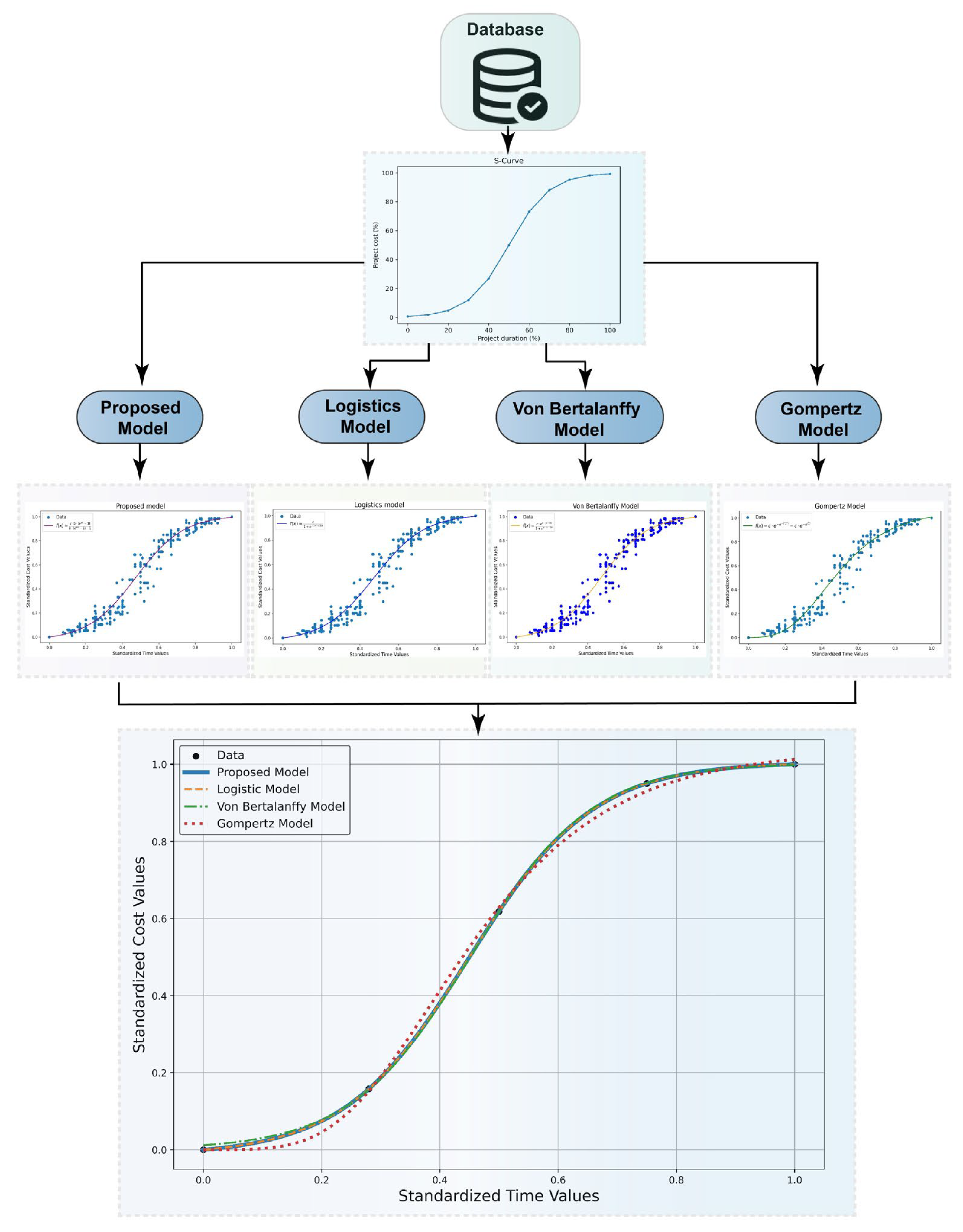
Figure 2.
Typical S-curve used in road projects.
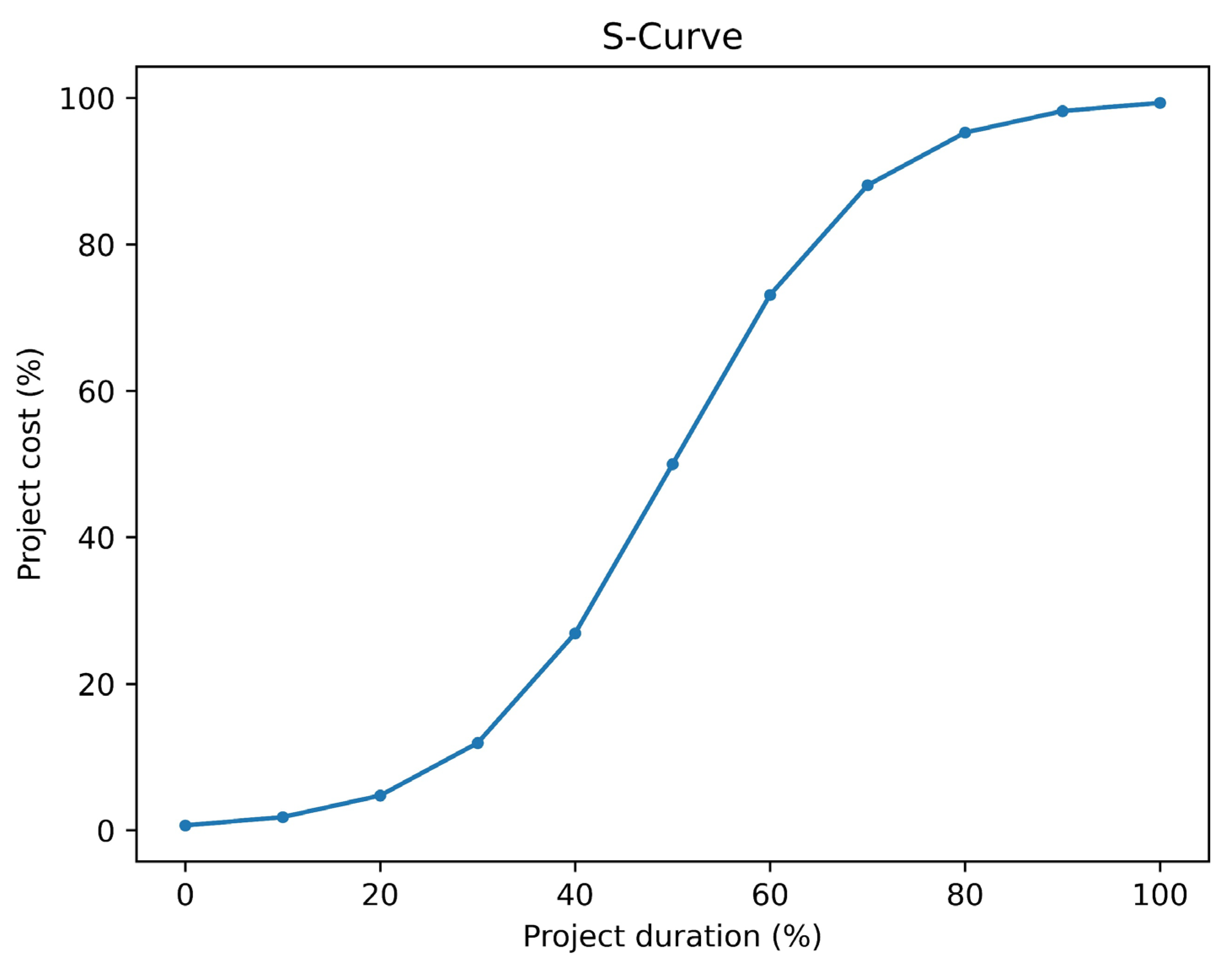
Figure 3.
Representative database projects.
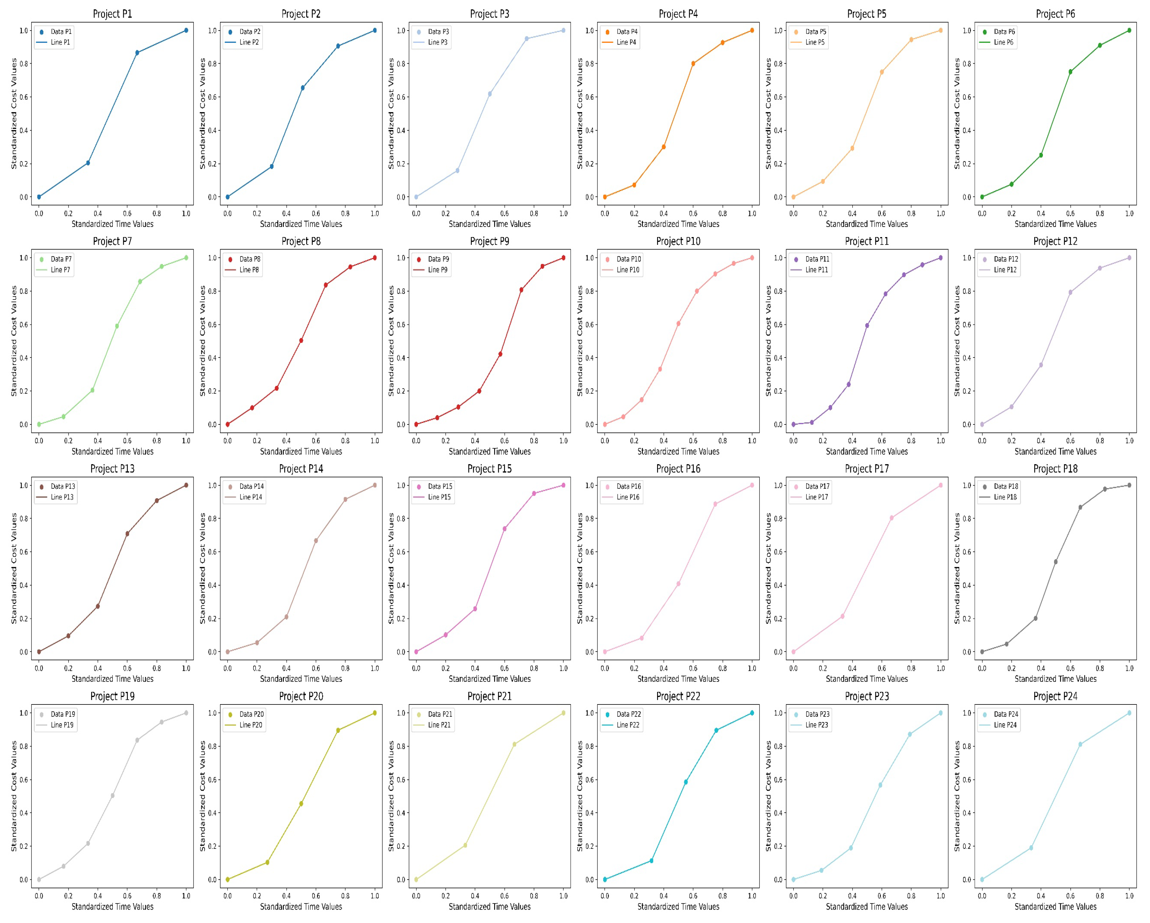
Figure 4.
Proposed model.
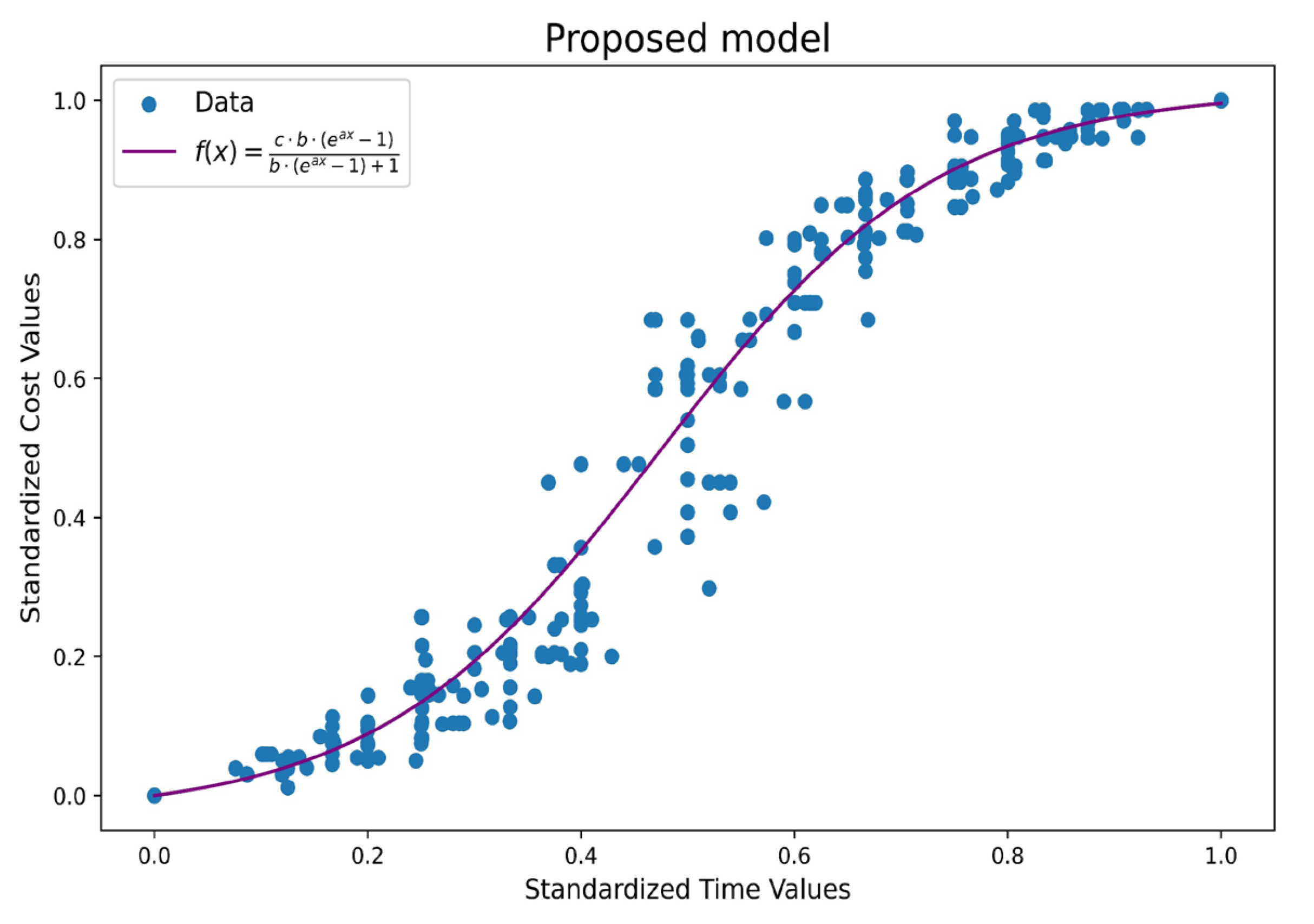
Figure 5.
Logistics model.
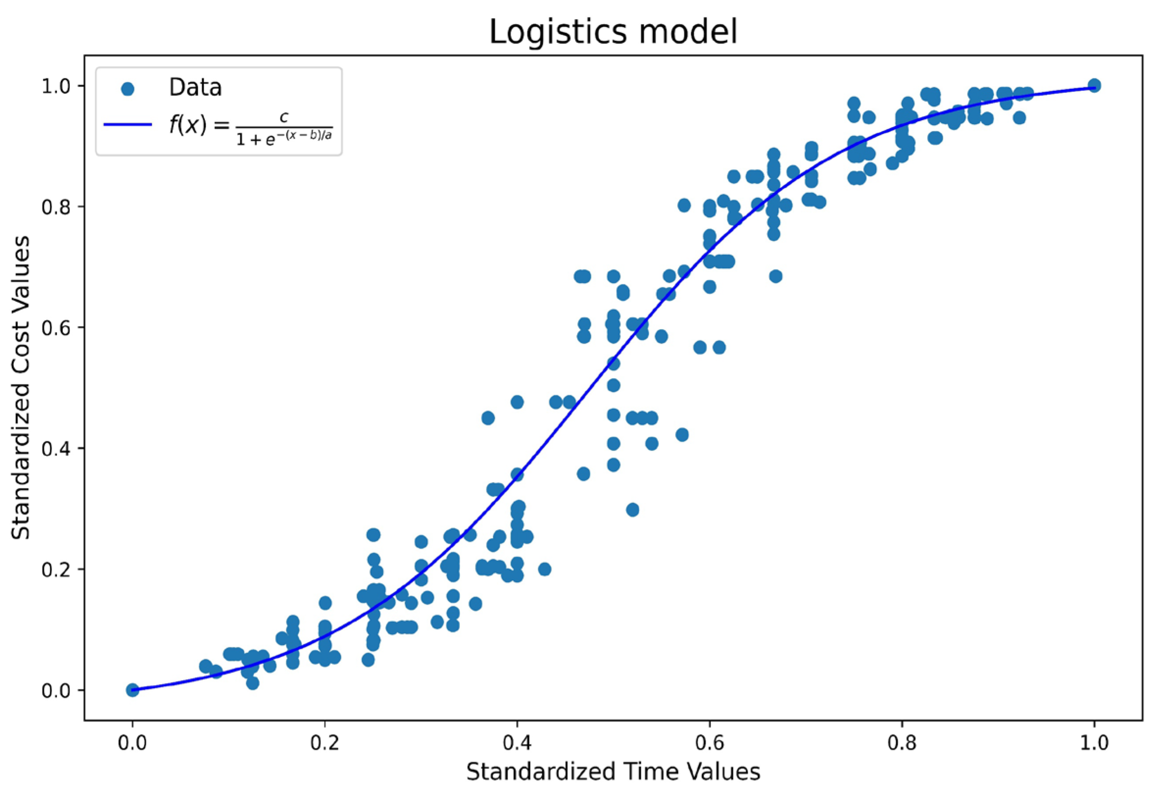
Figure 6.
Von Bertanlanffy Model.
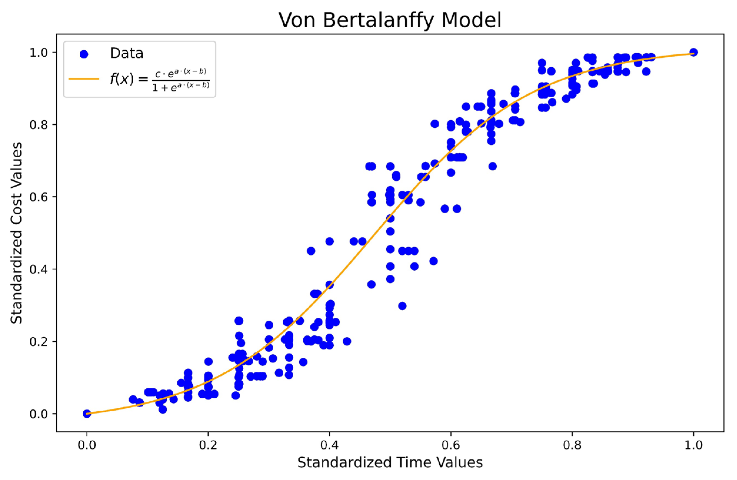
Figure 7.
Gompertz model.
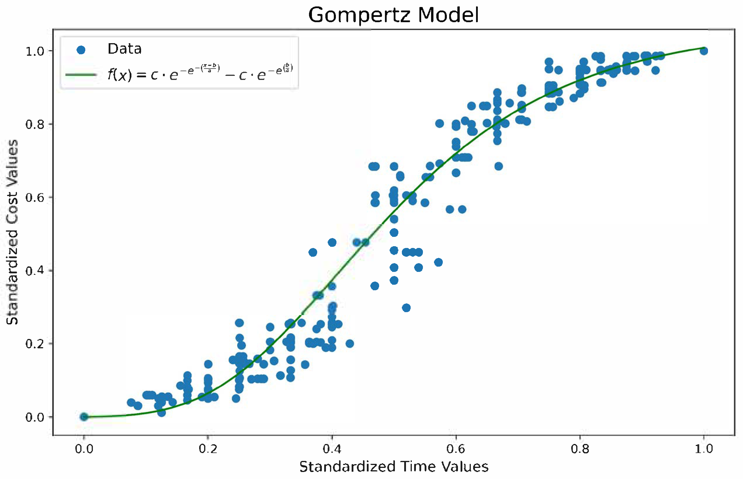
Figure 8.
Rigid pavement job planning database.
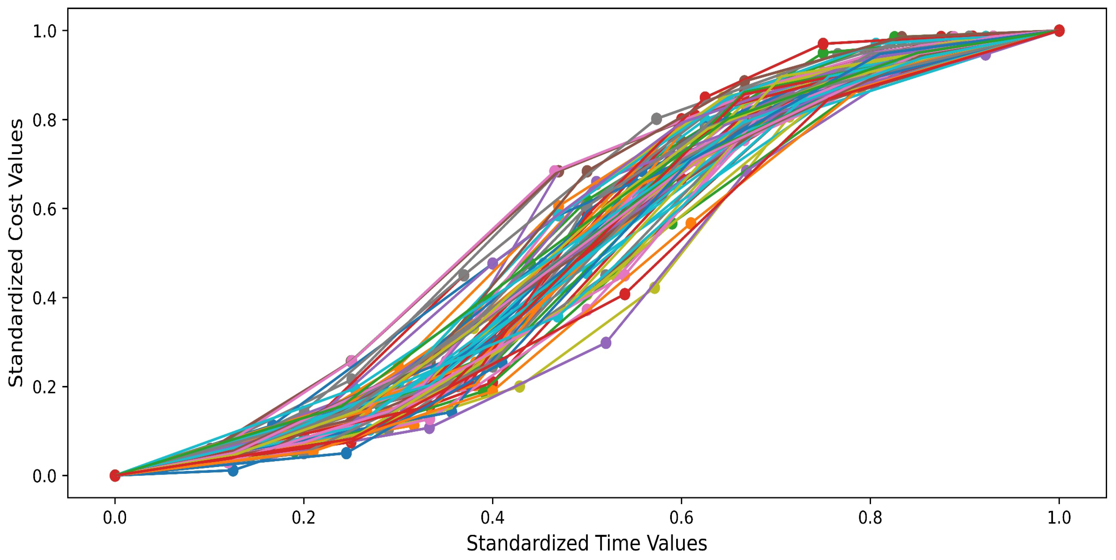
Figure 9.
(a) Proposed Sigmoidal Model, (b) Logistic Model, (c) Von Bertalanffy Model, and (d) Gompertz Model.
Figure 9.
(a) Proposed Sigmoidal Model, (b) Logistic Model, (c) Von Bertalanffy Model, and (d) Gompertz Model.
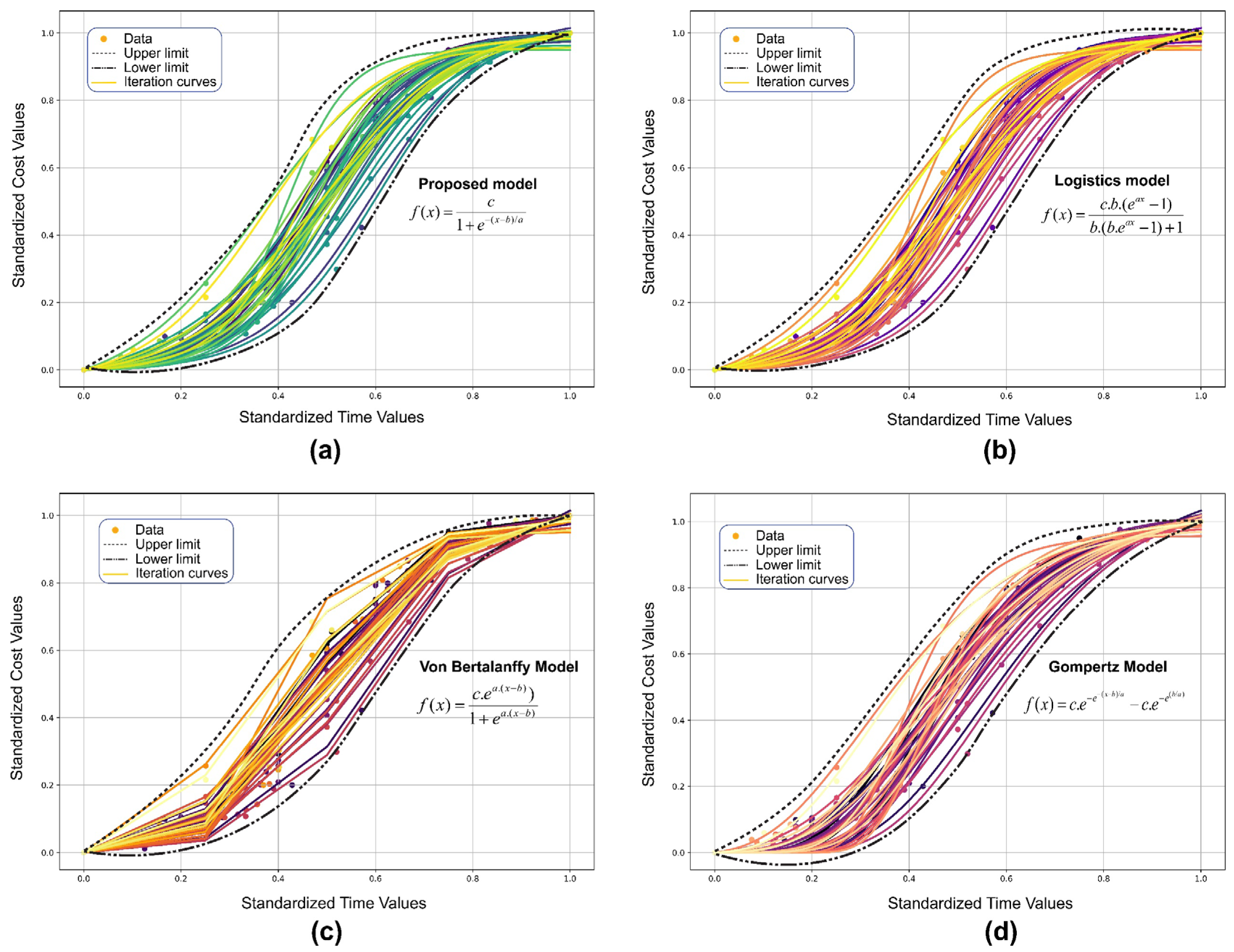
Figure 10.
Application of the different sigmoidal models for rigid pavement planning.
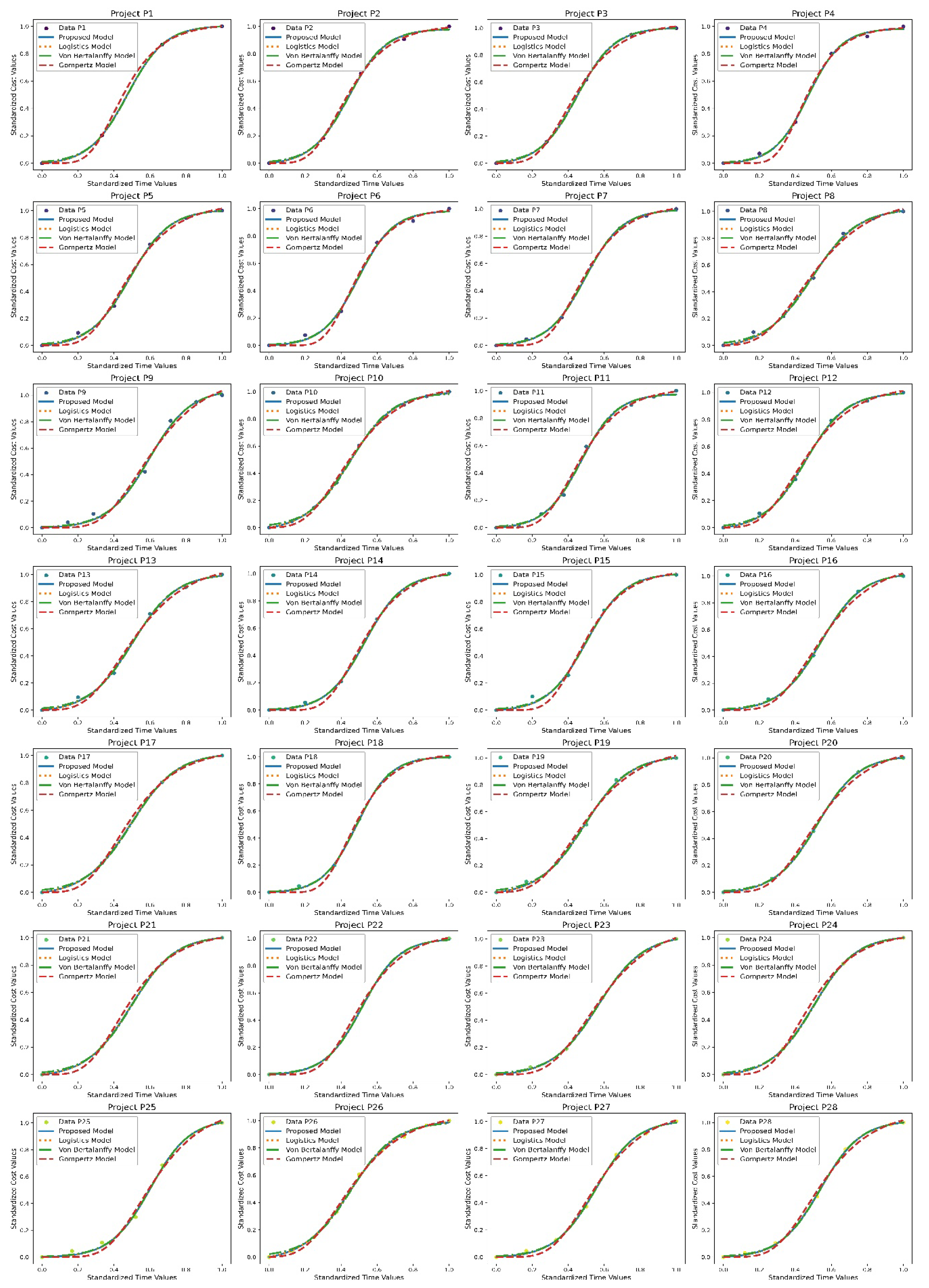
Table 2.
Descriptive statistics of the variables.
| Variable | Count | Mean | Standard Deviation | Minimum | 25% | 50% | 75% | Maximum |
|---|---|---|---|---|---|---|---|---|
| Time (Month) |
718 | 2.87 | 2.13 | 0.00 | 1.00 | 3.00 | 4.00 | 8.00 |
| Cost (US$) | 718 | 2556345.00 | 3344270.00 | 0.00 | 446702.70 | 1669521.00 | 3311307.00 | 24470880.00 |
Table 3.
Parameter estimation of the Proposed, Logistic, Von Bertalanffy, and Gompertz sigmoidal models.
Table 3.
Parameter estimation of the Proposed, Logistic, Von Bertalanffy, and Gompertz sigmoidal models.
| Parameter | Proposed model |
Logistics model |
Von Bertalanffy model |
Gompertz model |
|---|---|---|---|---|
| a | 1.5202 | 0.1096 | 9.4850 | 0.1682 |
| b | -62.9902 | 0.4800 | 0.4834 | 0.4217 |
| c | 70.7842 | 1.0020 | 0.9991 | 1.0433 |
Table 4.
Evaluation of sigmoidal models.
| Statistician | Proposed model |
Logistics model |
Von Bertalanffy model | Gompertz model |
|---|---|---|---|---|
| R | 0.9910 | 0.9924 | 0.9923 | 0.9917 |
| R2 | 0.9821 | 0.9848 | 0.9844 | 0.9832 |
| MSE | 0.0026 | 0.0026 | 0.0026 | 0.0028 |
| RMSE | 0.0506 | 0.0506 | 0.0512 | 0.0531 |
| MAE | 0.0278 | 0.0278 | 0.0321 | 0.0311 |
| AIC | -3386.0481 | -3386.0521 | -3373.5261 | -3346.3187 |
Disclaimer/Publisher’s Note: The statements, opinions and data contained in all publications are solely those of the individual author(s) and contributor(s) and not of MDPI and/or the editor(s). MDPI and/or the editor(s) disclaim responsibility for any injury to people or property resulting from any ideas, methods, instructions or products referred to in the content. |
© 2025 by the authors. Licensee MDPI, Basel, Switzerland. This article is an open access article distributed under the terms and conditions of the Creative Commons Attribution (CC BY) license (http://creativecommons.org/licenses/by/4.0/).
Copyright: This open access article is published under a Creative Commons CC BY 4.0 license, which permit the free download, distribution, and reuse, provided that the author and preprint are cited in any reuse.


