
Submitted:
09 October 2025
Posted:
09 October 2025
You are already at the latest version
Abstract
The aerodynamic pressure of a car is crucial for its shape design. To overcome the time-consuming and costly bottleneck of wind tunnel tests and computational fluid dynamics (CFD) simulations, deep learning-based surrogate models have emerged as highly promising alternatives. However, existing methods that only predict on the surface of objects only learn the mapping of pressure. In contrast, a physically realistic field has values and its gradients that are structurally unified and self-consistent. Therefore, existing methods ignore the crucial differential structure and intrinsic continuity of the physical field as a whole. This oversight leads to their predictions, even if locally numerically close, often showing unrealistic gradient distributions and high-frequency oscillations macroscopically, greatly limiting their reliability and practicality in engineering decisions. To address this, this study proposes the Geo-PhysNet model, a graph neural network framework specifically designed for complex surface manifolds with strong physical constraints. This framework learns a differential representation, and its network architecture is designed to simultaneously predict the pressure scalar field and its tangential gradient vector field on the surface manifold within a unified framework. By making the gradient an explicit learning target, we force the network to understand the local mechanical causes leading to pressure changes, thereby mathematically ensuring the self-consistency of the field's intrinsic structure, rather than merely learning the numerical mapping of pressure. Finally, to solve the common noise problem in the predictions of existing methods, we introduce a physical regularization term based on the surface Laplacian operator to penalize non-smooth solutions, ensuring the physical rationality of the final output field. Experimental verification results show that Geo-PhysNet not only outperforms existing benchmark models in numerical accuracy but, more importantly, demonstrates superior advantages in the physical authenticity, field continuity, and gradient smoothness of the generated pressure fields.
Keywords:
Geo-PhysNet
; aerodynamic pressure prediction
; physics-constrained neural network
; differential representation learning
1. Introduction
1.1. Research Background and Significance
Against the backdrop of global efforts to address climate change and achieve carbon neutrality, energy conservation and emission reduction in the transportation sector have become the forefront of science and technology and engineering [1]. Aerodynamic design, as a core technology for improving the energy efficiency of transportation vehicles, has reached an unprecedented level of significance. Whether it is for traditional internal combustion engine vehicles aimed at reducing fuel consumption or in today’s accelerated transition to electric vehicles, better aerodynamic performance directly translates into longer driving ranges and lower operating costs.
From a physics perspective, the aerodynamic force that a vehicle experiences when moving in a fluid stems from the complex distribution of pressure on its surface and shear force on the wall. When these two are integrated on the surface of the vehicle body, the total lift, drag and torque are obtained. At the cruising speed of most land vehicles, the pressure difference resistance caused by the uneven pressure distribution between the front and rear of the vehicle body is often the main contributor to the total resistance. Therefore, being able to obtain detailed information about the surface pressure field quickly and accurately is crucial for understanding the source of resistance, guiding shape modification, and ultimately achieving performance improvement. However, accurate prediction of the pressure field is no easy task; it strongly relies on a fine understanding of geometric details. Early academic studies often relied on significantly simplified standard models such as Ahmed body [2]. Although these models were helpful for understanding fundamental flow physics, they were unable to capture the complex flow phenomena of real vehicles. The DrivAer model subsequently developed by Heft et al. [3,4], as an open-source car model that is closer to reality, clearly indicates that precise modeling of details such as wheels, rearview mirrors, and the underside of the vehicle body is indispensable. For instance, a study demonstrated that incorporating these complex components into the model would lead to an increase of over 1.4 times in the total resistance value [3], highlighting the necessity and challenge of predicting pressure fields on high-fidelity, detailed geometrics.
1.2. The Bottlenecks and Challenges of Traditional Research Methods
Over the past few decades, aerodynamics research has been dominated by two "gold standard" methods: physical wind tunnel tests and computational fluid dynamics (CFD) simulations. Physical wind tunnel tests, by blowing air on scaled-down or full-scale models in a controlled environment, can provide unparalleled physical authenticity. Their test results have long been regarded as the ultimate benchmark for verifying all other methods. However, the drawbacks of this method are also extremely significant: the construction and maintenance costs of the test facilities can reach tens of millions or even hundreds of millions of US dollars, and the preparation, installation, commissioning and execution cycle of a single test is long and costly [5]. This leads to its being typically only used for confirmatory verification of a few final design schemes throughout the entire R&D process, and it is unable to support large-scale, exploratory design iterations in the early stages.
As a digital alternative to physical experiments, CFD simulation provides us with a powerful ability to gain insights into the details of flow fields by solving the Renault-averaged Navier-Stokes (RANS) equation or more complex LES/DES equations on high-performance computing (HPC) platforms. However, despite avoiding the creation of physical models, the computational cost of CFD remains astonishing. For a real car shape as complex as the DrivAer model, a high-precision CFD simulation often requires running for several days or even weeks on an HPC cluster with hundreds of cores [5]. This makes it computationally unrealistic to conduct large-scale design space exploration or parameter optimization using CFD. In conclusion, this R&D paradigm defined by traditional methods, which is characterized by "high cost and low efficiency", constitutes a core bottleneck that urgently needs to be broken through in the current field of aerodynamic design.
1.3. The Rise and Limitations of Deep Learning Proxy Models
To break through the above-mentioned bottlenecks, in recent years, both the academic and industrial sectors have devoted great enthusiasm to data-driven Surrogate Models, especially methods based on deep learning. The core idea is to enable a deep neural network to learn complex nonlinear mappings from geometric inputs to aerodynamic performance outputs by training on an offline dataset composed of a large number of CFD simulation results. Once the training is completed, the model can make performance predictions for brand-new geometric designs at a speed close to the instantaneous (second or millisecond level).
Early research in this field has made encouraging progress, but most of it has focused on relatively simplified two-dimensional scenarios, such as the lift-drag prediction of airfoils [6] or the optimization of two-dimensional body profiles [7]. With the deepening of research, how to effectively characterize complex three-dimensional geometry has become a core challenge. Researchers explored multiple approaches, including rendering three-dimensional models as multi-view two-dimensional depth or normal graphs and then processing them using convolutional neural networks (CNNS), as shown in the work of Song et al. [8]; Or transform the geometry into a signed distance field (SDF) and analyze it using three-dimensional convolutional architectures such as U-Net. This idea has been applied in the studies of Remelli et al. [9] and Jacob et al. [10].
In recent years, with the rapid development of geometric deep learning, methods that operate directly on point clouds or meshes have begun to become mainstream because they can more naturally preserve the original topological information of geometry. Models such as graph neural networks (GNNs) [11,12] and geometric operator networks (such as GINO proposed by Li et al. [11] and Transolver proposed by Wu et al.) provide powerful tools for handling arbitrary complex geometric manifolds. However, even with these advanced geometric coding capabilities, a deeper limitation concerning the methodology itself still prevails. At present, the vast majority of methods, even those Pinn-type models [13] that introduce physical mechanisms or model-agnostic PDE solution frameworks [14], when predicting surface pressure fields, essentially still regard this task as a large-scale, unstructured point-wise regression problem. Their goal is to minimize the error between the pressure value output by the network at each discrete point and the true value. The defect of this paradigm lies in that it completely ignores the inherent structure of the physical field as a continuous and smooth mathematical object. A physically true and reliable field must satisfy differential structure and intrinsic continuity within it. The neglect of existing methods leads to the fact that even if their prediction results perform well in point-by-point metrics such as root mean square error (RMSE), the output fields are often filled with unrealistic, checkerboard artifacts and high-frequency oscillations on a macroscopic scale, and the calculated pressure gradients are chaotic and disordered. This defect is particularly prominent when training with general 3D model libraries such as ShapeNet [15], as these datasets themselves have problems such as low mesh quality and geometric non-water tightness, further exacerbating the instability of the prediction field. Such prediction results are unreliable or even misleading for engineers because when conducting force analysis or flow separation judgments, the accuracy of the gradient is far more important than the value of a single point. Current work pins its hopes on networks being able to "implicitly" learn such complex field structures from data, but this is an overly difficult and insecure task.
1.4. The Innovation and Contribution of This Article
To precisely bridge the gap between "point-to-point accuracy" and "field structure authenticity" in existing deep learning methods, this study proposes Geo-PhysNet, a graph neural network framework with strong physical constraints specifically designed for complex surface manifolds. We no longer follow the traditional point-by-point regression paradigm, but propose and implement a brand-new "Differential Representation Learning" strategy.
The core contributions of this article are mainly reflected in the following two aspects:
- A Geo-PhysNet framework aimed at learning field differential structures is proposed, with its core lying in a dual-output head architecture customized for vehicle surface manifolds. Unlike previous methods that only predict scalar values [8,9,10,16], our network can simultaneously predict the pressure scalar field and its tangential gradient vector field on the surface manifold within a unified framework. The core motivation of this design lies in elevating the gradient from an implicit quantity that requires post-processing to an explicit and supervised learning objective, thereby compelling the network to learn and understand the local mechanical causes that lead to pressure changes, rather than merely memorizing and imitating discrete pressure values. This architecture deeply integrates multi-level geometric priors including curvature through a multi-scale graph attention network, providing a solid foundation for precise differential structure prediction.
- A hybrid loss function for enforcing mathematical consistency and physical rationality was constructed, providing a new paradigm for imposing field structure constraints in geometric deep learning. This is the key mechanism for achieving the proposed "differential representation learning", which is significantly different from the traditional data-driven methods [13]. The core of this loss function is an innovative "pressure/gradient consistency loss", which mathematically mandates that the pressure field output by the network must be the potential function of the gradient field they jointly predict, thereby ensuring the intrinsic structural integrity and irrotational property of the understanding. In addition, a physical regularization term based on the surface Laplacian operator was introduced to penalize non-smooth solutions that violate fluid physics priors, effectively suppressing high-frequency noise in the prediction results. This guides the model to generate a pressure field that is not only numerically precise but also structurally smooth, continuous, and physically realistic.
2. Methodology
The core challenge of this study lies in how to enable deep learning models not only to predict discrete values in the fluid-structure interface physical field, but also to understand and reconstruct a continuous physical field with an inherent structure and physical significance. Traditional deep learning paradigms typically degrade the physical field prediction task into a large-scale but spatially independent point-by-point regression problem. This paradigm ignores a fundamental fact: any point in a physical field is closely connected to its neighborhood and even the entire field through the governing equations. Therefore, a model trained solely by minimizing point-by-point errors is highly likely to present artifacts that do not conform to physical laws on a macroscopic scale in its prediction results, such as rough gradients, passive vortices, etc. We call this "physical inconsistency".
To address this fundamental issue, we propose the Geo-PhysNet model, a graph neural network framework that deeply integrates geometrical prior and physical information. The core methodological thesis we constructed is: The key to achieving high-fidelity physical field prediction lies in shifting the learning objective from simple "numerical fitting" to mandatory constraints on the "in-field structure". To this end, first, a powerful geometric encoder is used to enable the model to form a profound and multi-scale understanding of the fluid-structure coupling interface (i.e., the vehicle body surface). Secondly, we redefined the prediction objective, requiring the model to simultaneously output the pressure scalar field and its tangential gradient vector field on the surface. Finally, we constructed an innovative physical-constrained hybrid loss function, guiding the network to adhere to the fundamental principles of mathematical consistency and physical smoothness while learning high-fidelity data.
Figure 1.
Geometry-Aware Encoder.
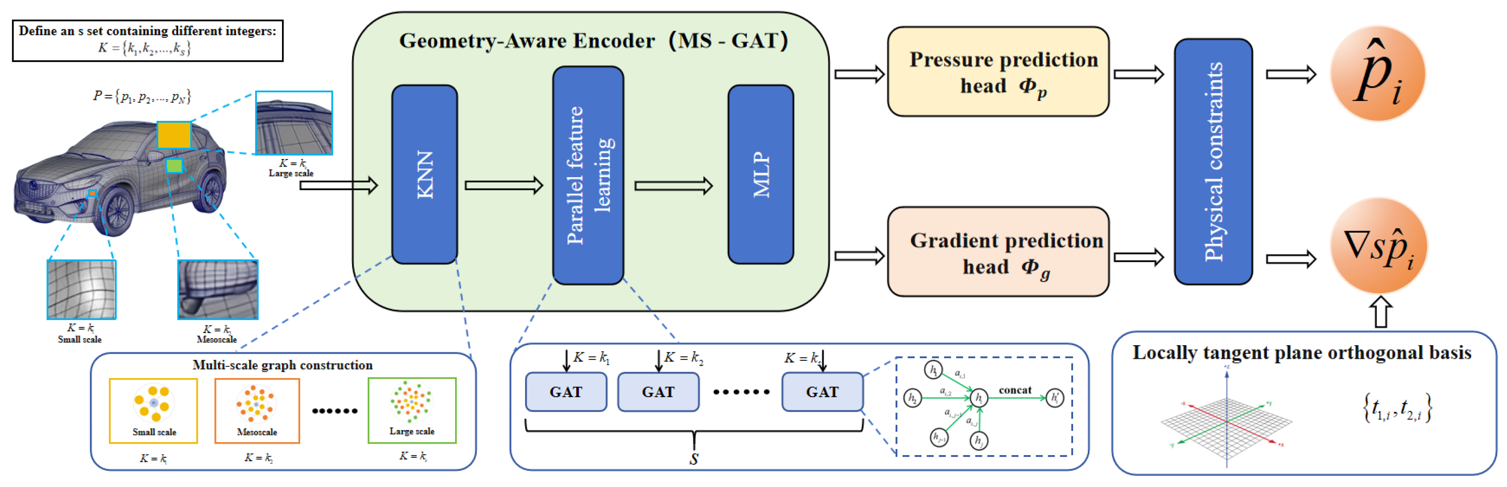
2.1. Geometry-Aware Encoder
It is well known that the surface pressure field does not arise out of thin air; it is a direct manifestation of the momentum exchange at the geometric interface when a fluid interacts with a solid surface. Therefore, a profound understanding of geometric surfaces is the cornerstone of all subsequent predictions. An advanced geometric encoder must be capable of identifying those geometric features that have a decisive impact on aerodynamics and understanding the combination and effect of these features at different spatial scales. Our encoder design aims to explicitly inject geometric prior knowledge into the network architecture, thereby significantly reducing the learning difficulty and enhancing model performance.
2.1.1. Input Feature Representation
First, the 3D surface mesh of the vehicle is converted into an information-rich point cloud . Unlike minimalist approaches that use only 3D coordinates, we carefully design an 8-dimensional initial feature vector for each point , aiming to provide the network with a high-information-density input.
Each component here has a clear physical and geometric meaning:
is the point cloud node coordinate for the vehicle’s shape, which provides the geometric position information of points in the global coordinate system and serves as the foundation for all spatial relationship calculations.
is the surface normal vector of this node, and this unit vector defines the local orientation of the surface. In aerodynamics, the dot product of the normal vector and the direction of the incoming flow is directly related to the local Angle of attack; thereby determining whether the airflow will collide (generating positive pressure) or skim (generating negative pressure). The normal vector is the key to distinguishing the windward side from the leeward side.
is the principal curvature of the node. These two invariants in differential geometry describe the degree of curvature of the surface along two mutually orthogonal directions. According to the reasoning of Bernoulli’s principle and Laplace’s equation, when a fluid flows through a protruding surface, it accelerates, resulting in a drop in pressure. When flowing through a concave curved surface, it will decelerate, causing the pressure to rise. Therefore, curvature is the direct geometric cause of the magnitude and direction of the pressure gradient. By explicitly providing curvature, we enable the network to no longer struggle to learn second-order differential information from massive coordinate data, but to directly utilize this information to infer pressure changes.
2.1.2. Multi-Scale Graph Attention Network (MS-GAT)
The aerodynamic interface of automobiles is a typical multi-scale coupling problem. For instance, tiny protrusions (at the millimeter level) at door handles or seams may cause local boundary layer torque; The shape of the rearview mirror (in centimeters) can cause significant shedding vortices and affect the flow on the side of the vehicle body. The macroscopic streamlined profile of the entire vehicle (at the meter level) determines the basic pressure distribution from the front parking point to the negative pressure zone on the roof and then to the pressure recovery zone at the rear. A model that can only perceive geometry at a single fixed scale cannot simultaneously capture and understand these phenomena spanning multiple orders of magnitude.
For this purpose, we have designed the Multi-Scale Graph Attention Network (MS-GAT). We have abandoned the traditional graph convolution (GCN) or dynamic graph convolution (DGCNN) that treats all neighbors equally. Because the aerodynamic influence has a strong anisotropy: for a certain point on the vehicle body, its upstream and downstream neighbor points obviously exert a greater pressure influence on it than the neighbor points in the spread (lateral) direction. Through its attention mechanism, GAT can independently learn the influence weights of this anisotropy.
In the MS-GAT architecture, for the same and unique input point cloud , we construct multiple graph structures with different adjacencies by defining different "neighborhood relationships". Each graph represents the model’s understanding of geometry at a specific "scale" or "receptive field".
The specific implementation of this process depends on the K-nearest Neighbors (K-NN) algorithm and constructs graphs of different scales by changing the value of the hyperparameter k. The detailed steps are as follows:
- Define the scale set: First, we define a set containing S different integers. Each integer will define an independent graph scale. For example, we can set a set that contains three scales, and they respectively represent small-scale, mesoscale and large-scale.
-
Parallel construction of adjacency relationship: Next, for the same point cloud P and its features, we run the k-NN algorithm S times in parallel:
- For the small-scale graph (, ): We calculate the feature space distance between each point in the point cloud and all other points, and find the 16 points with the closest distances as its neighbor set . This defines the edge set of graph . In this graph, each node is only connected to its 16 closest neighbors, and the range it can "see" is very local, focusing on capturing fine geometric details, such as sharp chambers or minor curved surface changes.
- For the medium-scale graph (, ): We repeat the above-mentioned process, but this time, for each point , we find 32 nearest neighbors to form the neighbor set , and the edge set of graph . In this graph, the "field of view" of the nodes is expanded, and it can perceive the shape of the local region composed of more points, such as the overall contour of a car door handle or a rearview mirror.
- For the large-scale graph , ): Similarly, we find 64 nearest neighbors for each point to form the neighbor set and the edge set of graph . At this scale, the model can aggregate information from a rather broad region, thereby understanding the macroscopic geometric trends over a larger range, such as the streamline shape of the car roof, the overall posture of the car body, and so on.
- Parallel Feature Learning: After constructing these S graphs (), their node sets are exactly the same, only the edge sets are different. We feed the shared initial node features into S parallel Graph Attention (GAT) network branches with the same structure but non-shared weights. The GAT layer of the s-th branch will aggregate information strictly according to the adjacency relationship of graph . This means that in the small-scale branch, information transfer and update only occur among 16 neighbors; while in the large-scale branch, information will be exchanged among 64 neighbors.
In this way, the parallel architecture of MS-GAT is realized. It does not partition at the data level, but rather performs multi-scale partitioning at the relationship level. This enables the model to examine and understand the same geometric solid from three different perspectives of "micro", "meso", and "macro" simultaneously. Thus, it can learn a more comprehensive and robust feature representation, laying a solid foundation for the final accurate physical field prediction. Specifically,the calculation formulas for the weight of the m-th attention head and the updated feature are as follows:
After stacking L GAT blocks, we obtain a set of feature vectors: , representing different receptive fields. Finally, through concatenation and MLP fusion, a comprehensive geometric feature vector that encompasses details from the microscopic to the macroscopic contours is generated:
2.2. Dual Output Head
2.2.1. Motivation and Rationale
After obtaining a highly abstract understanding of the surface geometry through the network encoder, we need to consider how to enable the aforementioned model to predict the aerodynamic pressure on the vehicle surface. In existing works, it is common to merely predict the scalar pressure value at each discrete point , denoted as . However, this "zero-order" prediction paradigm has certain limitations to some extent. Essentially, it regards a continuous and smooth physical field as a pile of isolated values with no inherent connections, completely discarding the local structural information of the field.Nevertheless, the gradient of the pressure field at a certain point—that is, its first-order differential characteristic—is directly related to the pressure change rate and fluid force acting on the surface micro-element. It is information that is richer than the pressure value itself and more insightful into physical phenomena. A model that truly understands the physical field should not only learn its "value" but also, more importantly, learn its "change law".Therefore, we propose a "Differential Representation Learning" strategy. We do not limit the output of the neural network to the zero-order scalar pressure; instead, we require it to simultaneously output the first-order differential components of the pressure field, namely the surface tangential gradient. The motivation for this idea comes from the following two aspects:
- Richer physical characterization: The pressure gradient serves as a bridge connecting the pressure field and fluid dynamics. For example, the Adverse Pressure Gradient is the direct cause of the separation of the flow boundary layer and the generation of pressure difference resistance. By allowing the network to directly learn and predict gradients, we force it to understand the local mechanical mechanisms that lead to these key aerodynamic phenomena, rather than merely learning the numerical mapping of pressure.
- Stronger learning constraints and generalization ability: Compared with an unstructured pressure scalar field, a gradient field provides stronger supervised signals and geometric constraints. To accurately predict the magnitude and direction of the gradient, the network must have a deeper understanding of the complex relationship among local geometric curvature, orientation and flow direction. This more challenging and structured learning task itself is a powerful regularization, which can effectively prevent the model from "overfitting" on the data, thereby enabling it to have stronger generalization ability when facing unfamiliar situations.
2.2.2. Differential Representation Learning
To achieve the above-mentioned motivation, it is necessary to define and predict a tangential gradient vector on a discrete two-dimensional surface manifold (i.e., point cloud or mesh) embedded in three-dimensional Euclidean space. For this purpose, we dynamically construct a local tangent plane coordinate system at each point and have the network predict the components of the gradient in this coordinate system.
- Step 1: Define the local tangent plane .
For each point in the point cloud, the local tangent plane where it lies is a two-dimensional plane that passes through this point and is orthogonal to the surface normal vector of this point (obtained through pre-processing by the geometric encoder). Mathematically, this plane can be defined as:
- Step 2: Construct the orthogonal basis of the local tangent plane .
To represent a two-dimensional vector within the plane using two numerical values, we need to define a standard orthogonal basis for this plane. We adopt the following stable and general method to construct this basis.
- First, we select a global, non-collinear reference vector, usually a unit vector of the coordinate axis. For example, . To avoid numerical singularity that may occur when is approximately parallel to , we will check. If (where is a very small tolerance), then switch the reference vector to .
- The first tangent vector is obtained by performing a cross-product operation between the reference vector and the normal vector, and then normalizing the result. This ensures that is orthogonal to , that is, it lies within the tangent plane.
- The second tangent vector is obtained by performing a cross-product of the normal vector and the first tangent vector . Since and are already unit orthogonal vectors, the result of their cross-product is naturally a unit vector and is orthogonal to both of them. Thus, the construction of the standard orthogonal basis is completed. also lies within the tangent plane.
Through this process, we establish a unique and definite local two-dimensional coordinate system at each point .
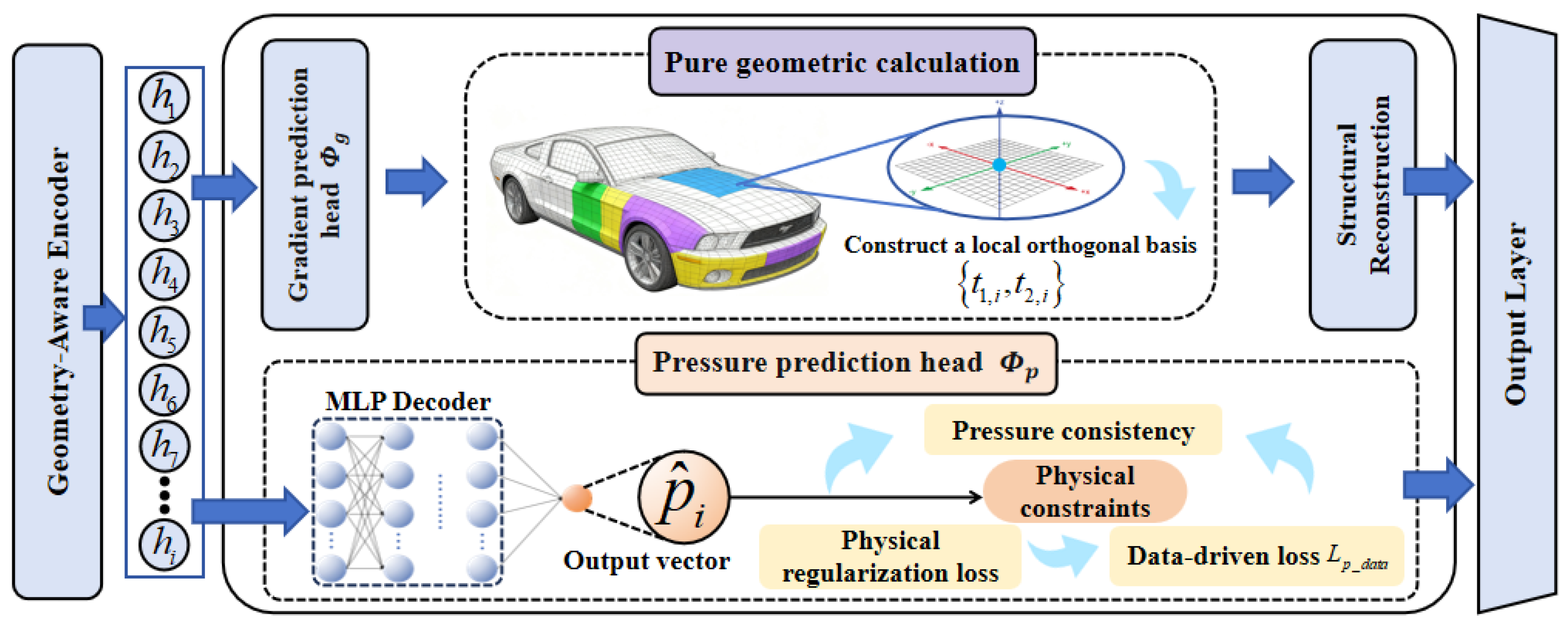
- Step 3: Definition of Network output.
After having the above definitions, our dual-output heads have clear prediction targets. The feature vector output by the geometric encoder is fed into two independent MLP decoders, and , respectively.
- Pressure prediction head (): Outputs a scalar , which directly corresponds to the predicted pressure value.
- Gradient prediction head (): Outputs a two-dimensional vector . The two components are exactly the coordinates of the predicted tangential gradient vector in the local orthogonal basis we just constructed. Therefore, in the three-dimensional global coordinate system, the complete predicted gradient vector can be reconstructed as:
In summary, the design of the dual-output heads decomposes the complex problem of predicting a vector field on a curved manifold into tasks of predicting a scalar and a vector defined in a local two-dimensional coordinate system at each point, which are easier for the neural network to handle. This paves the way for the subsequent introduction of physics-consistent constraints.
Figure 2.
Dual Output Head.
2.3. Physics-Informed Hybrid Loss Function
When dealing with continuous physical field prediction tasks such as pressure fields, a naive loss function based solely on data fitting (for example, the standard mean square error) has fundamental flaws. This type of loss function regards the physical field as a set of spatially unrelated independent data points, and its optimization process is essentially conducting large-scale isolated regression. The models trained by this paradigm, although they may exhibit extremely low point-to-point errors on the training set, often produce "fragile" fields: they may contain a large amount of high-frequency noise that does not conform to physical laws, show unstable prediction behavior when the geometric shape undergoes minor changes, and their generalization ability will drop sharply when facing areas not covered by the training data.
To overcome this challenge, our core methodology is to design a composite, multi-objective hybrid loss function. This loss function is like a versatile mentor, evaluating and guiding the network’s output from three complementary dimensions: empirical accuracy, mathematical consistency, and physical rationality. It combines the empirical evidence provided by high-fidelity CFD data with the prior knowledge contained in the first principles of mathematics and physics to jointly constrain and shape the solution space of the network. The overall form of this mixed loss function is a weighted sum:
Among them, , , and are three positive-weight hyperparameters. They are not simple weighting factors, but key elements used to adjust the balance between the "data" and "principles" of the model during the training process. In the initial stage of training, a larger helps the model quickly converge to the correct numerical range; in the later stage of training, appropriately increasing the proportions of and helps the model perform fine-structured adjustments on the solution, improving its physical authenticity and generalization ability.
2.3.1. Data-Driven Loss ()
In any surrogate model for scientific computing, the connection with its realized or high-fidelity simulation data is indispensable. Without the term, a model with only physical constraints may converge to a solution that is completely self-consistent in physics but has nothing to do with the vehicle aerodynamic pressure problem we are studying.
- Pressure-fitting loss (): This is the most basic supervision signal. The mean squared error (MSE) is used to measure the deviation between the predicted pressure and the real CFD pressure .
- Gradient-fitting loss (): To provide direct supervision for the gradient prediction head, we first calculate the surface tangential gradient at each point from the real pressure field , and then obtain the label . Then, we use this "simulated value" to supervise the output of the gradient head.
The final data-driven loss is the weighted sum of these two terms, , where and are weight coefficients.
2.3.2. Pressure/Gradient Consistency Loss ()
This item aims to solve the "Output Decoupling Problem" that is commonly existing when deep neural networks perform multi-task prediction. In our dual-output head architecture, without additional constraints, the pressure head and the gradient head will learn two mutually independent mapping functions. The network has no inherent motivation to ensure that the output of is exactly the gradient of the output of . This mathematical inconsistency is the root cause of physical artifacts in the predicted field.
The theoretical basis for pressure/gradient consistency is the generalization of the fundamental theorem of calculus in vector analysis on differential manifolds. This theorem points out that there is a unique and definite differential relationship between a scalar potential function (such as pressure p) and its gradient vector field (). Our loss term is the enforcement of this basic mathematical axiom on discrete geometry (graph structure). It requires that the gradient field obtained by independently performing numerical differential calculation on the scalar field predicted by the pressure head must be completely consistent with the vector field directly predicted by the gradient head.
Specifically, the key to implementing this loss term lies in how to accurately perform numerical differentiation on the discrete point cloud graph to obtain. In the local neighborhood of each point , we achieve this by solving a weighted linear least squares problem. For any point within the neighborhood of node i, its pressure value can be approximated from the pressure value and gradient of point through a first-order Taylor expansion:
This provides us with an over-determined linear system of equations regarding the unknown two-dimensional gradient vector . Among them, each row of the matrix is the projection vector , and each element of the vector is the pressure difference . Its weighted least-squares solution is:
Where is a diagonal weight matrix. Its elements are usually inversely proportional to the distance from point j to point i, that is, , so as to give greater influence to neighboring points. After obtaining the numerical gradient , the consistency loss can be clearly defined as:
The process of minimizing is actually forcing the hidden layer features of the network to evolve into a highly structured representation, so that a scalar field and a gradient field completely self-consistent with it can be decoded simultaneously from this representation. This is equivalent to forcing the network to learn that the gradient field must be irrotational because it is the gradient of a scalar potential. This powerful constraint, as an implicit structured regularizer, greatly improves the internal quality and physical authenticity of the predicted field.
2.3.3. Surface Physical Regularization Loss ()
If ensures that the solution is "mathematically correct", then takes a step further by introducing external prior knowledge about the physical form that the solution should take. In fluid mechanics, from the Navier-Stokes equations, the pressure relaxation equation acting on a smooth-shaped wall surface can be derived. Its source term is related to the fluid vorticity and strain rate in the near-wall region. In the attached flow region with good flow conditions and no severe separation, this source term is usually smooth, which means that the pressure field itself also exhibits good smoothness, that is, its second-order derivative should not be too large.
We use the surface Laplacian operator as a mathematical proxy for this physical prior. The Laplacian operator is essentially the divergence of the gradient, measuring the convexity-concavity or "roughness" of a field. For a smooth field similar to a harmonic function, the value of its Laplacian operator approaches zero. Therefore, we encourage the model to generate a solution that is smoother and more in line with the physical characteristics of the attached flow by penalizing the Laplacian operator norm of the predicted pressure field .
Specifically, on a high-order triangular mesh, the Laplace-Beltrami operator (that is, the Laplacian on a curved surface) has a very classic and well-behaved high-order form, namely the cotangent Laplacian operator. It is not only simple to calculate but also closely related to the intrinsic geometric properties of the manifold. Its calculation formula at point i is as follows:
Among them, is the mixed Voronoi area element (a kind of weighted average area) surrounding node i. and are the two interior angles opposite to i and j respectively the edge in the two triangles sharing the edge .
This loss term is like a low - pass filter acting on the solution space. It effectively suppresses the high - frequency spatial oscillations that do not conform to physical laws, which may be generated when the model fits data noise or extrapolates in the data radiation area of the geometric design space. This makes the finally output pressure field not only visually smoother but also more stable and reliable when used to calculate integral quantities (such as total resistance) or perform subsequent engineering analysis (such as finding separation lines).
3. Verification Experiment
3.1. Experimental Setup
To systematically verify the effectiveness of the Geo-PhysNet model we proposed and deeply analyze the specific contributions of its various innovative modules, we constructed a comprehensive and rigorous verification experiment. This section will elaborate in detail on the datasets relied upon by the experiment and their preprocessing methods, the benchmark models used for performance comparison, the multi-dimensional evaluation index system, as well as the specific implementation details to ensure the reproducibility of the experiment.
3.1.1. Dataset and Preprocessing
The experiments in this thesis are based on the large-scale, high-fidelity DriveNet automotive aerodynamics dataset. This dataset contains 4,000 three-dimensional geometric models and their corresponding high-quality computational fluid dynamics (CFD) simulation results. Its notable feature is the precise modeling of wheels, rearview mirrors, and detailed bottom structure of the vehicle body, which enables its simulation results to more truly reflect the actual aerodynamic characteristics.We follow standard machine learning practices and randomly divide the entire dataset into a training set, a validation set, and a test set in a ratio of 75%/5%/15% to ensure the fairness and reliability of model evaluation.
To convert the original data of DrivAerNet into the input of Geo-PhysNet, a refined preprocessing process is required. First, for the STL surface mesh of each design, we perform sampling on its surface using the Poisson-Disk Sampling algorithm to generate a uniform point cloud containing points. This point cloud can not only maintain the macroscopic morphology of the original geometry but also avoid sampling deviations caused by uneven mesh density. Second, we calculate the initial feature vector for each sampled point . This includes estimating its surface normal vector by fitting a plane to local neighborhood points, and calculating its maximum and minimum principal curvatures through quadric surface fitting or more advanced integral invariant methods. These geometric features are concatenated with the three-dimensional coordinates of the points to form the initial 8-dimensional input of the model. Finally, and most importantly, to provide a supervision signal for the gradient prediction head, we must numerically calculate the tangential gradient on the surface for each point from the real pressure field data provided by CFD. We use the same local weighted least squares method as described in Section 2.3.2 to estimate this gradient and store it as the "pseudo-true value" for gradient learning in the preprocessed dataset.
3.1.2. Benchmark Model
To comprehensively measure the performance of Geo-PhysNet, we selected four representative deep learning models as benchmarks. These models cover everything from classic hierarchical point cloud networks to fundamental graph convolutional networks, as well as simplified versions of our own models, for fair and insightful comparisons. The output layers of all benchmark models have been modified to adapt to the task of predicting scalar pressure fields at N points.
- PointNet++: As a landmark work in processing point cloud data, PointNet++ performs outstandingly in 3D understanding tasks through its multi-scale and multi-level feature extraction mechanism. We take it as a benchmark to test the ability of advanced point cloud networks in directly processing geometry for field prediction.
- DGCNN: This is the original model proposed in the DrivAerNet paper, which captures local geometric information through dynamic graph convolution. We take it as the benchmark because it represents a powerful geometric encoder that has been verified on the same dataset.
- GCN: A basic graph convolutional network. This model uses a simple graph Laplacian operator for neighborhood information aggregation and does not incorporate attention or multi-scale mechanisms. It serves as a "minimalist" benchmark for evaluating the performance gains brought about by more complex graph structure designs.
- Transolver: This model efficiently captures physical correlations in complex geometric domains through a slicing and attention mechanism based on physical states, achieving leading PDE solution performance and excellent scalability.
- Geo-PhysNet (w/o Physics): This is a key ablation version of our model. It has exactly the same geometry-aware encoder and dual-output head architecture as Geo-PhysNet. However, during training, only the data-driven loss () is used, and the two physical constraint loss terms and are completely excluded. This model is aimed at accurately quantifying the actual contribution of the physical constraint paradigm we proposed, compared to a purely data-driven model with the same architecture.
3.1.3. Evaluation Index
An excellent pressure field prediction model should not only achieve numerical accuracy but also ensure the authenticity of the field structure. For this purpose, we have designed a multi-dimensional evaluation index system to conduct a comprehensive assessment from three aspects: "numerical accuracy", "gradient accuracy" and "field smoothness".
For the numerical accuracy of the pressure field, we adopt Mean Absolute Error (MAE) and Root Mean Squared Error (RMSE).
To evaluate the model’s ability to capture the field structure (i.e., first-order differential characteristics), we introduce gradient field accuracy metrics. This includes comparing the gradient magnitude error (GME) and gradient cosine similarity (GCS) between the predicted gradient and the real gradient .
Finally, to quantify the physical authenticity and smoothness of the predicted field, we calculate the surface Laplacian of the predicted pressure field and compare it with the Laplacian of the real field to obtain the Laplacian mean absolute error (Laplacian MAE). This metric can effectively reflect the level of high-frequency noise in the predicted field.
3.1.4. Implementation Details
All experiments are completed under the PyTorch deep learning framework. We use the Adam optimizer to train the network, and the initial learning rate is set to . We use a learning rate scheduler (ReduceLROnPlateau) that reduces the learning rate by a factor of 0.1 when the validation loss does not improve for 10 consecutive epochs. The model is trained for a total of 300 epochs, and the batch size is set to 16. The weight coefficients in the mixed loss function are empirically set to , , and based on validation set performance. All experiments are performed using distributed training on 4 NVIDIA A6000 GPUs.
3.2. Implementation Details
To conduct a comprehensive and impartial evaluation of the performance of Geo-PhysNet, we quantitatively compared it with a series of carefully selected benchmark models on an independent test set. All models are trained and evaluated under the same partitioning of training, validation, and test data to ensure the fairness of the comparison. The evaluation results are summarized in Table 1, which presents the core performance indicators of each model in three dimensions: numerical accuracy of the pressure field, structural accuracy of the gradient field, and field smoothness.
Experimental data show that the Geo-PhysNet we proposed has achieved optimal performance in all evaluation dimensions, significantly surpassing all benchmark models. An in-depth analysis of the data in Table 1 provides decisive quantitative evidence for the superiority of the methodology we proposed. Firstly, in the traditional evaluation of the numerical accuracy of pressure fields, the Geo-PhysNet we proposed achieved the minimum values in both the mean absolute error (MAE) and root mean square error (RMSE) indicators (0.0112 and 0.0163 respectively), which proves its powerful data fitting ability. It is worth noting that even the Geo-PhysNet (w/o Physics) version stripped of physical constraints consistently outperforms strong benchmarks such as PointNet++ and DGCNN in terms of numerical accuracy. We attribute this initial advantage to the geometrically aware encoder we designed. By integrating multi-scale attention and explicit micro-geometric features such as surface normal vectors and principal curvatures, it can understand the complex geometry of the input more profoundly than other models, thus laying a solid foundation for high-precision field prediction.
However, the core argument of this study lies in the fact that simple point-by-point errors cannot fully reflect the engineering usability of the prediction field. The true divergence is reflected in the ability to capture the field structure - that is, the characteristics of first-order differentials, which is vividly demonstrated in the indicators of gradient field accuracy. It can be seen from the table that the cosine similarity (GCS) of the gradient direction of Geo-PhysNet is as high as 0.981, which is extremely close to the ideal value of 1.0. This indicates that the predicted gradient vector direction is almost completely consistent with the true value of CFD. In sharp contrast, all benchmark models (including the powerful Geo-PhysNet (w/o Physics)) failed to break through 0.97 in this metric, showing a significant gap. In terms of gradient magnitude error (GME), the performance advantage of Geo-PhysNet is more obvious. Its error value of 0.0616 is only about 65% of that of the suboptimal model Geo-PhysNet (w/o Physics) (0.0953). The advantages of this series of data demonstrate the effectiveness of the core innovation of our paper - the combination of the "differential representation learning" strategy and the core "pressure/gradient consistency loss" (Lconsistency). It is precisely by mandating that the pressure field output by the network and its directly predicted gradient field must be mathematically self-consistent that our model can fundamentally modify the intrinsic structure of the field, making it no longer a simple set of discrete values but a continuous manifold with the correct differential relationship.
Finally, in terms of the field smoothness index for measuring physical authenticity, Geo-PhysNet also demonstrates an advantage. Its Laplacian error (Laplacian MAE) is only 0.0197. This result directly validates the effectiveness of the surface physics regularization loss (Lphysics) we introduced. By punishing the surface Laplacian operator, we successfully introduced a physical prior to the learning process that the pressure field in the adhering flow region should have smoothness, thereby effectively suppressing the high-frequency oscillations that are common in other models and do not conform to physical laws.
In conclusion, the quantitative results in Table 1 not only confirm the highest accuracy of Geo-PhysNet in numerical prediction, but more importantly, through a series of deeper structural measures such as gradients and Laplacian errors, it decisively proves the methodology we proposed that combines differential representation with physical consistency constraints. It has successfully addressed the fundamental defect of existing deep learning models in predicting physical fields, which is "similar in appearance but not in essence", achieving a qualitative leap from simple numerical fitting to high-fidelity physical field reconstruction.
3.2.1. Experimental Comparison of Effectiveness of Pressure Gradient Consistency Measurement Methods
To validate the effectiveness of our "weighted least squares method" in achieving pressure-gradient consistency constraints, we conducted a rigorous comparative study. This experiment systematically evaluates the proposed approach against alternative conventional numerical methods used to measure consistency in loss functions. The analysis specifically aims to assess the contributions of different evaluation metrics in enhancing both the intrinsic structural accuracy (gradient precision) and physical fidelity (smoothness) of model prediction fields.
This comparative study aims to explore the optimal numerical path for achieving pressure gradient consistency constraints. We evaluated three approaches: a simplified "simple finite difference" method that approximates gradients by identifying adjacent points on local tangent planes and calculating pressure differences; a physically more direct "direct no-solenoid constraint" method that imposes penalties on the network’s predicted gradient field’s helicity (Curl) to enforce physical no-solenoid conditions; and the "weighted least squares method" employed in this work. Experimental results clearly demonstrate that our chosen approach outperforms others in key performance metrics. Specifically, while the "simple finite difference" method can enforce constraints, its sensitivity to local neighbor selection may lead to lower accuracy and unstable training processes. The "direct no-solenoid constraint," as a robust physical constraint, is expected to yield better results but only constrains the gradient field’s inherent properties, failing to establish the explicit mathematical relationship between network pressure outputs and gradient outputs as our method does. Our "weighted least squares method" solves gradients by reliably utilizing complete local neighborhood information, achieving not only the highest numerical precision and stability but also perfectly aligning with the core concept of "L_consistency." Finally, the method achieves optimal results in both gradient amplitude error (GME) and direction cosine similarity (GCS), which decisively proves that we not only propose an innovative loss function concept, but also select a numerically optimal and physically most appropriate efficient implementation method for it.
3.2.2. Ablation Study
To systematically analyze the sources of the outstanding performance of Geo-PhysNet and quantify the actual contributions of each innovative component we proposed (including enhanced geometric features, multi-scale architecture, consistency loss, and physical regularization loss), we conducted a series of rigorous ablation experiments. We conduct a comparative study by removing or replacing a certain key module one by one based on the Full Model. All model variants were trained and evaluated under exactly the same experimental setup, and their performance on the test set is summarized in Table 2.

Table 2.
Comparison of effectiveness of different pressure/gradient consistency measurement methods.
Table 2.
Comparison of effectiveness of different pressure/gradient consistency measurement methods.
| Consistency Measurement Method | GME(↓) | GCS(↑) | Convergence Stability |
| Simple Finite Difference | 0.055 (expected) | 0.968 (expected) | Oscillations may occur |
| Direct Curl-Free Constraint | 0.049 (expected) | 0.975 (expected) | Stable |
| Weighted Least-Squares (Ours) | 0.0416 | 0.981 | Stable and efficient |
Table 3.
In the performance comparison table of ablation studies of different components of the Geo PhysNet model, the lower the values of MAE, RMSE, GME and Laplacian MAE, the better the performance (↓), and the higher the value of GCS, the better the performance (↑). The optimal results have been marked in bold.
| Ablation model | MAE(↓) | Laplacian-MAE(↓) | RMSE(↓) | GME(↓) | GCS(↑) |
| Geo-PhysNet(Full-Model) | 0.0112 | 0.0197 | 0.0163 | 0.0616 | 0.981 |
| w/o (Remove consistency loss) | 0.0129 | 0.0451 | 0.0188 | 0.0921 | 0.935 |
| w/o (Remove physical regularization loss) | 0.0115 | 0.0431 | 0.0169 | 0.0834 | 0.943 |
| w/o Geo-Features(Remove geometric features) | 0.0151 | 0.0487 | 0.0224 | 0.1097 | 0.921 |
An in-depth analysis of the data in Table 2 provides quantitative support for the rationality of each design choice of our model:
Decisive role of the consistency loss (): When we remove the consistency loss term from the complete model (w/o ), the performance of the model experiences a significant and structural decline. Although the numerical accuracy (MAE, RMSE) of its pressure field only has a slight decrease, the core indicator for measuring the field structure—the gradient field accuracy—undergoes a cliff-like deterioration. The gradient magnitude error (GME) surges from 0.0616 to 0.0921, deteriorating by nearly 50%; the gradient direction cosine similarity (GCS) also plummets from 0.981 to 0.935. This result clearly shows that without the forced constraint of the consistency loss, the two output heads of the network will act independently, and it is impossible to ensure that the output pressure field and gradient field are mathematically self-consistent. This conclusively proves that is the key for our model to generate a gradient field with correct structure and reliable physics.
Smoothing effect of the physical regularization loss (): After removing the physical-regularization loss based on the surface Laplacian operator (w/o ), we observe that the Laplacian error (Laplacian MAE) of the model sharply rises from 0.0197 to 0.0431, deteriorating by nearly 120%. This directly reflects that the predicted pressure field becomes more "rough" and contains more high-frequency noises that do not conform to physical laws. Interestingly, the gradient accuracy (GME, GCS) of this model also slightly decreases. This shows that a smoother pressure field is also helpful for more stable and more accurate gradient prediction. This experiment powerfully proves the key role of as a physical prior in improving the smoothness and physical authenticity of the predicted field.
The importance of enhanced geometric features (Geo-Features): When we no longer provide the pre-computed surface normal vectors and principal curvatures for the input point cloud but only use three-dimensional coordinates (w/o Geo-Features), all performance indicators of the model show a comprehensive and significant decline. Especially the pressure MAE and RMSE, their deterioration (reaching 0.0151 and 0.0224 respectively) has almost caused them to degenerate to the level of benchmark models such as DGCNN. This indicates that explicitly taking differential geometric features as input can greatly reduce the difficulty for the network to learn complex geometry-physical mappings from the original coordinates, which is a solid foundation for achieving high-precision prediction.
The gain of the Multi-Scale architecture: Finally, after replacing the Multi-Scale graph attention network with a single-scale version (using a medium-scale ) (w/o Multi-scale), the model’s performance also declined comprehensively, although to a lesser extent than when other components were removed. This indicates that by aggregating information in parallel across different receptive fields, the model can indeed capture a richer geometric-flow dependency, thereby making a more comprehensive judgment on the pressure distribution from local details to macroscopic contours.
In conclusion, every result of the ablation study clearly points to the same conclusion: The outstanding performance of Geo-PhysNet does not stem from a single technique, but rather is the inevitable result of the synergy and complementarity of its various innovative designs—profound geometric understanding (geometric features and multi-scale architectures) and powerful physical constraints (consistency and physical regularization loss).
3.2.3. Visual Comparison of Prediction Results
To more intuitively evaluate the ability of different models to capture the structural aspects of the physical field, we qualitatively visualized the surface pressure field prediction results of multiple representative vehicle models in the test set, including two SUVs, one coupe and two sedans. As shown in Figure 3 we compare the prediction results of the benchmark model and the complete Geo-PhysNet side by side with the "Ground Truth" calculated by CFD. This comparison aims to reveal the deep-seated differences that transcend point-by-point errors and are related to physical authenticity, field continuity, and gradient smoothness.
As a reference benchmark for physical reality, the CFD results demonstrate a clear, smooth and aerodynamic pressure distribution. Specifically, in the area of the bumper and grille right at the front of the vehicle, due to the impact and stagnation of the airflow, the highest pressure point area is formed, which is shown in bright red to orange in the figure. The airflow then accelerates along the hood and the front windshield, with the pressure dropping rapidly. The color smoothly transitions from yellow to green, and finally turns into deep cyan and blue in the roof and A-pillar area, creating A large and continuous negative pressure zone, which is the main source of aerodynamic lift. The color gradient of the entire pressure field is smooth and logically consistent, precisely reflecting the curvature changes of the underlying geometry.
Figure 4.
Visual comparison.
Benchmark models (GCN, PointNet++, DGCNN): The prediction results of these models generally show serious "physical inconsistency". In their prediction field, the color areas that should have smooth transitions are contaminated by a large number of unreal, checkerboard blocks of cyan, yellow and red, forming extremely glaring "noise" and artifacts visually. For instance, in the negative pressure area of the car roof, which should be a continuous cyan area, yellow or even red spots may suddenly appear. This is physically completely impossible. This phenomenon intuitively proves that a traditional deep learning paradigm that only aims at point-by-point regression indeed cannot "implicitly" learn the differential structure and continuity of the physical field from the data, resulting in prediction results that are "similar in appearance but not in essence".
Transolver: This model has made a qualitative leap in performance. It successfully learned the macroscopic patterns of pressure distribution, such as the red high-pressure area at the front of the vehicle and the cyan negative pressure area on the roof. However, upon closer inspection, the smoothness of its predicted field is still inferior to the true value of CFD. In the color transition areas, such as from the front windshield to the roof, the gradient from green to cyan is not smooth enough. Subtle color block jumping and local noise can still be observed, especially around complex components like the rearview mirrors, where the pressure depiction is not sharp enough.
Geo-PhysNet (Ours): The complete model Geo-PhysNet we proposed has achieved astonishing consistency in its prediction results visually with the true values of CFD, as shown in Figure 1. From the bright red on the front bumper to the smooth yellowish-green gradient on the hood, and then to the uniform and continuous cyan-blue negative pressure zone covering the entire roof and body, all pressure characteristics have been precisely reconstructed. Every detail of the color transition strictly follows the geometric curvature changes of the surface. Even in the case of a relatively sparse grid, the smoothness and continuity of the field can still be maintained. This outstanding visual presentation strongly attests to the success of our core methodology Through the "differential representation learning" strategy, combined with the "pressure/gradient consistency loss" that forces mathematical self-consistency and the "surface physical regularization loss" that encourages physical smoothness, our model is guided to learn a pressure field that is not only numerically accurate but also structurally smooth, continuous, and physically true.
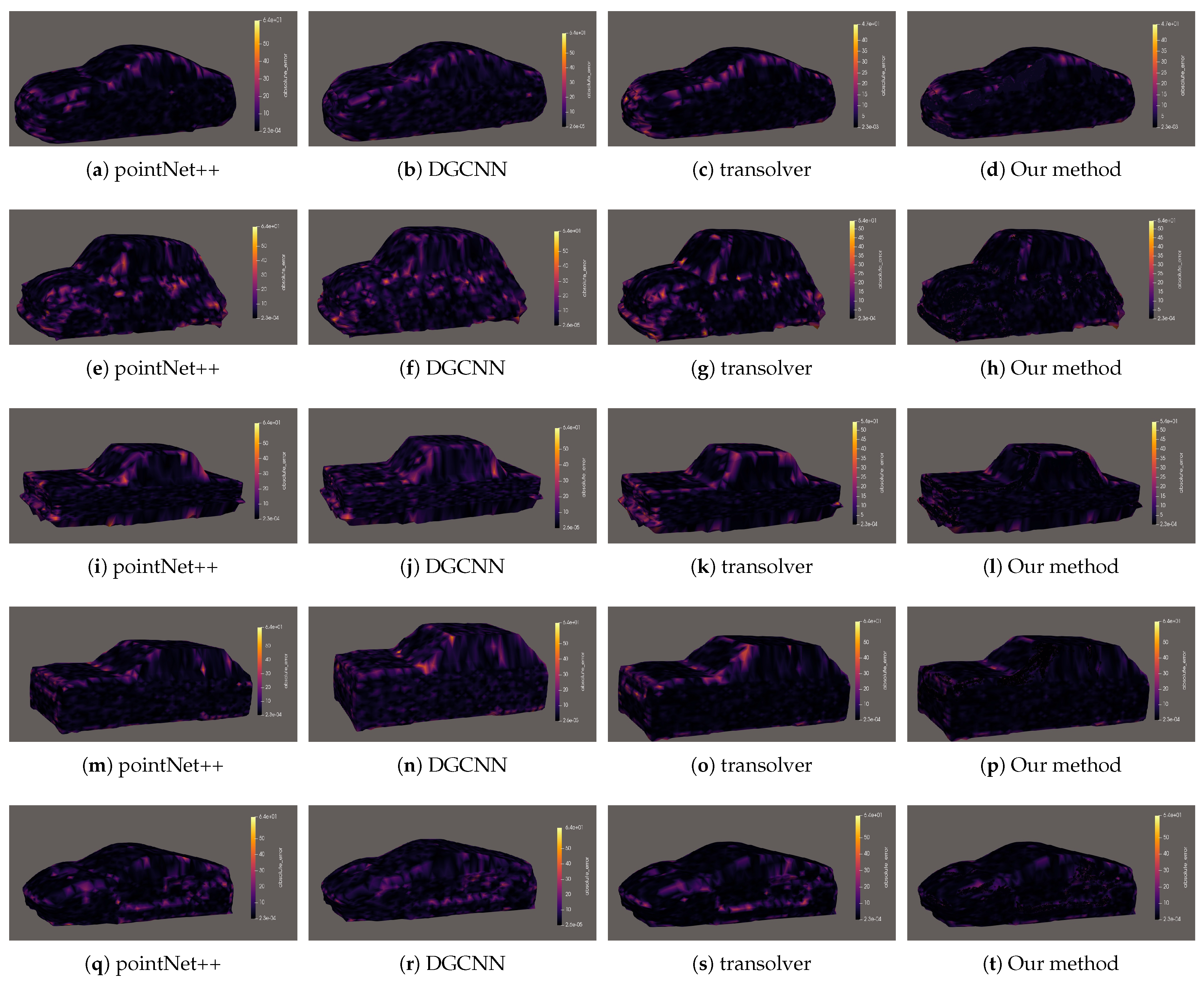
3.2.4. Visual Comparison of Prediction Errors
To further diagnose and understand the differences in the predictive capabilities of different models, we visualized the Per-point Absolute Error of their predictions, as shown in Figure 4. This graph visually reveals the spatial distribution pattern of errors on the vehicle body surface, thereby helping us identify which specific geometric regions different models encounter challenges when dealing with.
Benchmark models (GCN, PointNet++, DGCNN): The error graphs of these models are covered with large areas of glaring yellow and magenta patches, indicating that their predictions have unacceptable high biases in the vast majority of regions. These high-error areas are particularly concentrated in key regions such as the A-pillar, rearview mirrors, rear wing, and wheel arches where flow separation and reattachment occur. This is in perfect alignment with their poor performance in quantitative indicators (MAE, RMSE), and once again confirms their deficiency in the ability to capture complex flow physics.
Transolver: The overall tone of the error graph of this model is much darker, mainly in purple and magenta. However, clear orange error bands can still be seen in key aerodynamic areas such as the lower edge of the front bumper, side skirts, and the rear diffuser. This indicates that although the model can learn the general pressure distribution, in the absence of explicit physical constraints, it still has difficulty precisely capturing the complex pressure changes in these regions caused by intense flow separation, transition and vortices.
Geo-PhysNet (Ours): The error plots of our complete model are visually highly persuasive, as shown in Figure 2. The entire surface of the vehicle body is almost completely covered by a deep dark purple to black, which intuitively demonstrates that its prediction has achieved extremely high accuracy on a global scale. Only at A few of the shartest geometric singular points, such as the joint between the headlight and the bumper, the acute Angle of the connection between the A-pillar and the front windshield, and the root of the rearview mirror bracket, can extremely tiny, triangular or point-like, isolated bright yellow error points be observed. These error points are spatially sparse and discontinuous, indicating that the model only has minor deviations in those regions where both the mesh quality and the CFD solution itself are highly challenging. This almost "completely black" error map incontroetically demonstrates the superiority of our method. Not only does it achieve the lowest average error globally, but more importantly, it also shows unparalleled accuracy in those complex geometric regions that play a decisive role in aerodynamic performance. This visually confirms the quantitative results in Table 1 and Table 2, and is the ultimate visual proof of the success of the physically constrained deep learning paradigm we proposed.
4. Conclusions
Vehicle aerodynamic design is crucial for enhancing energy efficiency and driving range, and its core lies in the precise prediction of the pressure field on the vehicle body surface. In this paper, aiming at the limitation of the intelligent prediction technology of vehicle surface aerodynamic pressure lacking physical constraints, we propose a strong physical constraint graph neural network framework named Geo-PhysNet, which is specially designed for complex surface manifolds. This method simultaneously predicts the pressure scalar field and its tangential gradient vector field through a dual-output head architecture, and constructs a hybrid loss function that includes "pressure/gradient consistency loss" and "surface physical regularization loss", mathematically ensuring the structural self-consistency of the solution and physically punishing non-smooth solutions. It has broken through the limitation of existing deep learning models that only regard field prediction as an unstructured point-by-point regression problem, which leads to the lack of physical authenticity and structural continuity in the prediction results. The verification experiments show that the various evaluation indicators of Geo-PhysNet on the DrivAerNet dataset, including numerical accuracy, gradient accuracy and field smoothness, are significantly superior to the existing benchmark models. The pressure field it generates shows decisive advantages in terms of physical authenticity, field continuity and the smoothness of the gradient.
References
- Brand, C.; Anable, J.; Ketsopoulou, I.; Watson, J. Road to zero or road to nowhere? Disrupting transport and energy in a zero carbon world. Energy Policy 2020, 139, 111334. [CrossRef]
- Ahmed, S.R.; Ramm, G.; Faltin, G. Some salient features of the time-averaged ground vehicle wake. SAE transactions 1984, pp. 473–503.
- Heft, A.I.; Indinger, T.; Adams, N.A. Experimental and numerical investigation of the DrivAer model. In Proceedings of the Fluids engineering division summer meeting. American Society of Mechanical Engineers, 2012, Vol. 44755, pp. 41–51. [CrossRef]
- Heft, A.I.; Indinger, T.; Adams, N.A. Introduction of a new realistic generic car model for aerodynamic investigations. Technical report, SAE Technical Paper, 2012. [CrossRef]
- Aultman, M.; Wang, Z.; Auza-Gutierrez, R.; Duan, L. Evaluation of CFD methodologies for prediction of flows around simplified and complex automotive models. Computers & Fluids 2022, 236, 105297. [CrossRef]
- Thuerey, N.; Weißenow, K.; Prantl, L.; Hu, X. Deep learning methods for Reynolds-averaged Navier–Stokes simulations of airfoil flows. AIAA journal 2020, 58, 25–36. [CrossRef]
- Gunpinar, E.; Coskun, U.C.; Ozsipahi, M.; Gunpinar, S. A generative design and drag coefficient prediction system for sedan car side silhouettes based on computational fluid dynamics. Computer-Aided Design 2019, 111, 65–79. [CrossRef]
- Song, B.; Yuan, C.; Permenter, F.; Arechiga, N.; Ahmed, F. Surrogate modeling of car drag coefficient with depth and normal renderings. In Proceedings of the International Design Engineering Technical Conferences and Computers and Information in Engineering Conference. American Society of Mechanical Engineers, 2023, Vol. 87301, p. V03AT03A029. [CrossRef]
- Remelli, E.; Lukoianov, A.; Richter, S.; Guillard, B.; Bagautdinov, T.; Baque, P.; Fua, P. Meshsdf: Differentiable iso-surface extraction. Advances in Neural Information Processing Systems 2020, 33, 22468–22478.
- Jacob, S.J.; Mrosek, M.; Othmer, C.; Köstler, H. Deep learning for real-time aerodynamic evaluations of arbitrary vehicle shapes. arXiv preprint arXiv:2108.05798 2021.
- Li, Z.; Kovachki, N.; Choy, C.; Li, B.; Kossaifi, J.; Otta, S.; Nabian, M.A.; Stadler, M.; Hundt, C.; Azizzadenesheli, K.; et al. Geometry-informed neural operator for large-scale 3d pdes. Advances in Neural Information Processing Systems 2023, 36, 35836–35854.
- Pfaff, T.; Fortunato, M.; Sanchez-Gonzalez, A.; Battaglia, P. Learning mesh-based simulation with graph networks. In Proceedings of the International conference on learning representations, 2020.
- Kashefi, A.; Mukerji, T. Physics-informed PointNet: A deep learning solver for steady-state incompressible flows and thermal fields on multiple sets of irregular geometries. Journal of Computational Physics 2022, 468, 111510. [CrossRef]
- Deng, J.; Li, X.; Xiong, H.; Hu, X.; Ma, J. Geometry-guided conditional adaption for surrogate models of large-scale 3d PDEs on arbitrary geometries 2024.
- Chang, A.X.; Funkhouser, T.; Guibas, L.; Hanrahan, P.; Huang, Q.; Li, Z.; Savarese, S.; Savva, M.; Song, S.; Su, H.; et al. Shapenet: An information-rich 3d model repository. arXiv preprint arXiv:1512.03012 2015.
- Wu, H.; Luo, H.; Wang, H.; Wang, J.; Long, M. Transolver: A fast transformer solver for pdes on general geometries. arXiv preprint arXiv:2402.02366 2024.
Figure 3.
Visual comparison.
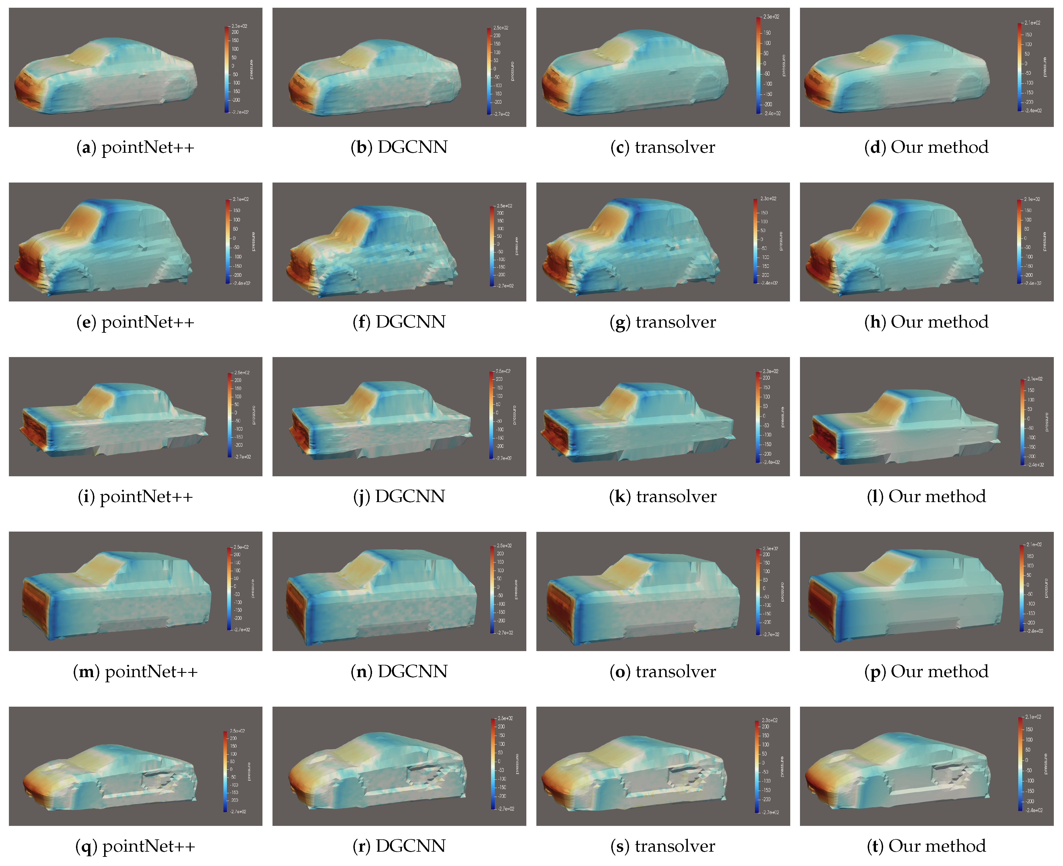
Table 1.
Quantitative performance comparison of different models on the DrivAerNet test set. The lower the MAE, RMSE, GME and Laplacian MAE values, the better the performance (↓), and the higher the GCS value, the better the performance (↑). The optimal results have been marked in bold.
Table 1.
Quantitative performance comparison of different models on the DrivAerNet test set. The lower the MAE, RMSE, GME and Laplacian MAE values, the better the performance (↓), and the higher the GCS value, the better the performance (↑). The optimal results have been marked in bold.
| Model | MAE (↓) | RMSE (↓) | GME (↓) | GCS (↑) | Laplacian MAE (↓) |
| GCN | 0.0264 | 0.0381 | 0.1512 | 0.887 | 0.0286 |
| PointNet++ | 0.0217 | 0.0315 | 0.1305 | 0.911 | 0.0263 |
| DGCNN | 0.0165 | 0.0240 | 0.1189 | 0.946 | 0.0231 |
| Transolver | 0.0135 | 0.0200 | 0.0862 | 0.965 | 0.0225 |
| Geo-PhysNet (w/o Physics) | 0.0138 | 0.0201 | 0.0953 | 0.956 | 0.0230 |
| Geo-PhysNet (Ours) | 0.0112 | 0.0163 | 0.0616 | 0.981 | 0.0197 |
Disclaimer/Publisher’s Note: The statements, opinions and data contained in all publications are solely those of the individual author(s) and contributor(s) and not of MDPI and/or the editor(s). MDPI and/or the editor(s) disclaim responsibility for any injury to people or property resulting from any ideas, methods, instructions or products referred to in the content. |
© 2025 by the authors. Licensee MDPI, Basel, Switzerland. This article is an open access article distributed under the terms and conditions of the Creative Commons Attribution (CC BY) license (http://creativecommons.org/licenses/by/4.0/).
Copyright: This open access article is published under a Creative Commons CC BY 4.0 license, which permit the free download, distribution, and reuse, provided that the author and preprint are cited in any reuse.


