Submitted:
07 October 2025
Posted:
09 October 2025
You are already at the latest version
Abstract
How to characterize the topological order of quantum spin liquids remains a long-standing theoretical challenge. In this work, we employ the pattern decomposition method to analyze the fine structure of the Kitaev spin liquid on a finite honeycomb lattice. The Kitaev Hamiltonian decomposes into six sub-Hamiltonians whose weight factors form periodic patterns under unit cell translations. Correspondingly, the eigenstates of the Kitaev spin liquid are partitioned into six degenerate subspaces, unveiling the ordered structure of the spin liquid state. The critical point of the topological phase transition from a gapped to a gapless phase is identified through the sub-Hamiltonians. This Hamiltonian dissection approach reveals the fine structure of the Kitaev spin liquid and offers a promising platform for the quantum simulation of spin liquids.
Keywords:
Kitaev spin liquid
; phase transition
; topological order
1. Introduction
In a crystal lattice, randomly oriented spins can spontaneously self-organize into collectively ordered states as the temperature decreases, such as ferromagnetic order with uniform magnetization or antiferromagnetic order with sublattice magnetization. These ordered states are characterized by local order parameters exhibiting translational symmetry. In contrast, quantum spin liquids lack any form of local order despite strong spinCspin interactions. Unlike the direct product state of disordered spins in a paramagnetic phase, the collective wavefunction of a quantum spin liquid is a highly entangled quantum state that hosts exotic quasiparticles obeying fractional statistics. The quantum spin liquid state was first proposed by Anderson in 1987 as the underlying mechanism for superconductivity of by Anderson in 1987 [1]. Later, an exact realization of a quantum spin liquid was theoretically established in the Kitaev honeycomb model, which supports non-abelian anyons in its gapless phase [2]..
Unlike the long-range order found in conventional magnetic phases, the spin-spin correlations in the gapless phase of the Kitaev spin liquid are strictly short-ranged [3,4,5,6]. This indicates that its intrinsic order is not captured by traditional magnetic correlations but is instead characterized by a topological invariant, namely the Chern number [2,3,7]. The application of an external magnetic field opens a gap in this gapless phase, thereby exciting pairs of anyons [8,9,10,11]. These anyonic excitations are of significant interest due to their potential application in topological quantum computation [12,13,14].
The iridium-based honeycomb oxides have been experimentally studied as candidate systems for realizing the Kitaev spin liquid, stimulating extensive research into both two-dimensional [15,16] and three-dimensional [17] material platforms for Kitaev-type models [18]. It was not until 2022 that a quantum spin liquid state was experimentally verified, with the observation of a U(1) quantum spin liquid in the triangular lattice magnet[19]. Moreover, Abelian anyons associated with spin liquids have been detected in fractional quantum Hall fluids via quantum interference experiments [20,21]. Nevertheless, the non-Abelian anyon expected in the Kitaev spin liquid remains experimentally elusive to date.
The gapped and gapless phases of the Kitaev spin liquid are characterized by zero and non-zero Chern numbers, respectively [2,3]. However, revealing the underlying topological order in the highly degenerate Kitaev spin liquid states remains a theoretical challenge. The collective pattern decomposition method for quantum spin Hamiltonians has proven effective in identifying quantum phase transitions in various many-body systems, including the quantum Rabi model [22], the quantum transverse Ising model [23,24], and the Heisenberg model [25]. In this approach, the total Hamiltonian is decomposed into a sum of sub-Hamiltonians, each contributing the energy of an individual pattern [24,25]. In this work, we employ the collective pattern decomposition method to uncover the fine structure of the Kitaev spin liquid state and use the density matrix renormalization group to locate the critical point of the phase transition associated with the sub-Hamiltonians.
2. The Pattern of Kitaev Model on Honeycomb Lattice
The Kitaev model on a finite honeycomb lattice consisting of 24 lattice sites is demonstrated in Figure 1. Both the horizontal and vertical bonding directions of the honeycomb lattice obey periodic boundary conditions, mapping the Kitaev model into intersecting spin chain loops on torus. The exact Hamiltonian of Kitaev model is consists of direction dependent spin-spin couplings,
The exact ground state energy is derived by mapping spins into Majorana fermions[2] or Jordan-Wigner transformation [3,4].
where is the momentum vector of electron on honeycomb lattice. The ground states are divided into the gapped phase and gapless phase. The spin-spin coupling parameters in the gapless phase satisfy the following inequalities,
Without losing generality for the following discussions, the parameters for the gapped phase is chosen as (), while the gapless phase is derived by the parameter setting, (, , ).
In Figure 1, there are 24 electrons in total locating at 24 lattices sites. Each electron carries three spin components to interact with its nearest neighbors. The quadratic Hamiltonian Equation (1) of the 24 electrons is the sum of Kitaev-type interacting bonds, which is reexpressed into a 72 by 72 matrix form,
Exact digonalization of the Hamiltonian matrix Equation (4) yields 6 independent eigenvalues, (), i.e., . Each of the six eigenvalue has 12 fold degeneracy. The th degenerated eigenvectors at the ith site with respect to the nth eigenvalue is denoted as , i.e., . For example, the first degenerate eigenvector with respect to the eigenvalue has only non-zero at .
Each electron at one site contributes its three spin components as three nearest neighboring elements to the 72 dimensional column vector in Equation (4). Since the interacting 24 particles are no longer free particles, a collective composite operator with respect to the nth eigenvalue is introduced to represent one collective pattern, which is expressed as the linear combinations of the spin components of 24 electrons, (; i = 1,2,...,24),
The coefficient in front of the spin operator measures its weight in the Hamiltonian. The total Hamiltonian Equation (1) is divided into 6 sub-Hamiltonian of the collective composite operator according to the six eigenvalues,
For example, the sub-Hamiltonian with respect to the first eigenvalue reads
The sub-Hamiltonian with respect to the second eigenvalue shares similar chain operator with , but carries different coefficients,
The total Hamiltonian describes six collective patterns, living in six subspaces expanded by 12 degenerated eigenvectors. Each composite operator generates a collective pattern with eigen-energy ,
where is the collective wave function of ground state. The eigenvectors with respect to expands 12 dimensional subspace. The coefficients of adjacent within the operator chain of composite operator (, , ) have the same sign (as shown in Equation (7)), representing a collective pattern in phase, which is named after the symmetric pattern. While the coefficients of adjacent within the composite operator (,,) have opposite signs (as shown in Equation (8)), representing a collective pattern out of phase, which is called the antisymmetric pattern. The 12 dimensional degenerated subspace with respect to an eigenvalue is further divided into two more 6 dimensional subspaces, the symmetric subspace and the antisymmetric subspace.
The ground state energy of the six sub-Hamiltonian evolves into different branches with coupling strength. In the gapped phase as showed in Figure 2 (a), the three energy branches, (, , ), grows with above zero, while the other two branches, (, ), show a monotonic growth below zero. The second energy branch decreases with , bringing the total energy to the minimal value. Therefore, subbranch dominates the evolution of Kitaev spin liquid. The same evolution behavior shows in the gapless phase in Figure 2 (b), the subbranch drops quickly to ground state with . But the energy gap between and and is highly suppressed. Therefore, the collective pattern of dominates the evolution of Kitaev spin liquid.
The eigenenergy with respect to the six sub-Hamiltonian are computed by numerical diagonalization with density matrix renormalization group. The six energy branches are obtained from energy Equation (9). Figure 3 (a) shows the overlapped energy branches, and evolves with coupling parameter , which agree with the cross section of the exact solution of energy spectrum in Figure 4. The branches shows a parabola curve with coupling parameter in Figure 3 (b). But the branch evolves against coupling strength shows two sudden dropping points around , indicating the phase transition point from gapped phase to gapless phase. The energy branches, and against coupling strength , also exist similar oscillating behavior around . According to the exact energy Equation (2), exchanging the with yields the same energy spectrum, resulting in the similar evolution behavior in Figure 3 (b), Figure 3 (c) and Figure 3 (d).
3. The Hexagon-Rhombus Visualization of Collective Pattern on Honeycomb Lattice
A more intuitive way of visualizing the collective patterns is to locate the three weight coefficients of three spin components at the lattice sites in real space. The weight coefficients at every lattice site is denoted as a vector,
As the exemplar Equation (7) and Equation (8) shows, only the sign of the weight coefficient changes in different pattern Hamiltonian. Therefore a filled or unfilled rhombus is chosen to label a positive or a negative , as showed in Figure 5 (b). Every weight coefficient vector at the ith site, , is represented by a hexagon composed of three rhombuses, as shown in Figure 5 (a). For the exemplar weight distribution of collective pattern in the left panel of Figure 5 (c), the dying internal rhombus of six hexagons at six lattice sites are explicitly visualized in the right panel of Figure 5 (c).
For the original Kitaev Hamiltonian Equation (4), most weight coefficients in front of spin operators are zero, due to the high degeneracy of eigenvectors induced by Kitaev coupling rules between nearest neighboring spins. In order to lift the degeneracy of the matrix eigenvalues of Kitaev Hamiltonian Equation (4), a small external field is applied along the three spin-spin coupling bonds,
The external field strengths along the three bonds are . These small external field does not change the exact ground state energy Equation (2) due to . In the numerical calculations, the small external field is set to . The highly degenerated ground state energy level is loosen into closely stacked energy bundles, which are far separated from the first excited state. The hidden collective patterns become more apparent after eliminating the degenerated zeros. However, the eigenvalues is no longer real number, but carries an imaginary part, which is still much smaller than the real part, indicating stable fine energy levels. The eigenvalues share the same absolute values with that without the external field. The sign of the real part of is labeled to the hexagon of three rhombuses to visualize the collective patterns. These stable collective patterns are independent of the specific values of external field.
The vectors with uniform signs translate to form collective pattern lattice in the gapped phase of Kitaev spin liquid. In the ferromagnetic phase in Figure 6 (a), all weight coefficients with respect to eigenvalue are positive, which are represented by uniformly dyed rhombus in red. In the antiferromagnetic pattern in Figure 6 (b), the rhombus triple within a hexagon are dyed in the same way. The nearest neighboring hexagons have opposite signs, demonstrating a similar antiferromagnetic order as classical Ising spins. Unlike the Ising model, the eigenvalues of the ferromagnetic and antiferromagnetic pattern are not the largest absolute values among all . Figure 6 (c) shows a striped phase, in which each row of fully dyed hexagon are all dyed in the same way, while the nearest neighboring rows are dyed in opposite ways. The nearest neighboring electrons may combine into a vertical dimer composed of two hexagons uniformly dyed in red, as shown in Figure 6 (d).
The collective pattern lattice composed of inhomogeneous vectors also exist as eigenvector of the sub-Hamiltonian. The vector cluster composed of two unfilled hexagons, one fully filled hexagon and one partly filled hexagon represents an unit cell with four electrons, which are enveloped by the red rectangle on the left-up corner in Figure 7 (a). The four vectors on the left-bottom corner is exactly dyed in an opposite way to that on the upper corner in Figure 7 (a). The two oppositely dyed vector clusters, as labeled by the red rectangle and the yellow rectangle in Figure 7 (a), form the unit cell of an antiferromagnetic lattice of collective pattern with respect to eigenvalue . Figure 7 (b) is a ferromagnetic pattern lattice of unit cluster with four partly filled hexagons, as showed by the four lattice sites on the left-up corner in Figure 7 (b), the eigenvalue of this ferromagnetic pattern is . The ferromagnetic pattern lattice of Figure 7 (c) with shares the same eigenvalue with Figure 7 (b), belonging to the same degenerated subspace. The ferromagnetic pattern lattice of Figure 7 (d) is generated by translation of unit cell of hexagon partly filled by , with respect to .
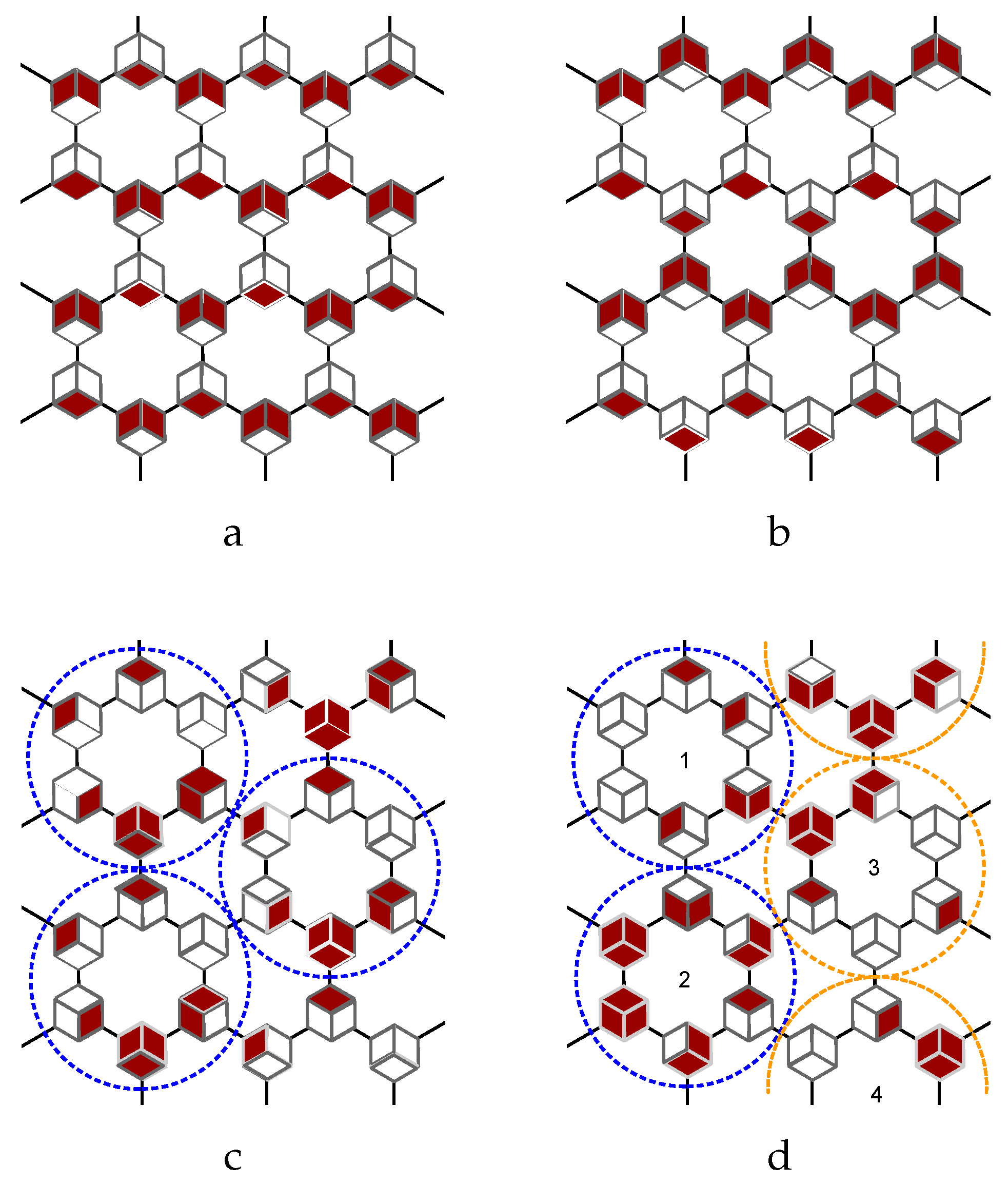
The kitaev spin liquid encodes more complex collective pattern lattice, that is generated by translating unit cell composed of six or twelve lattice sites. The unit cell of the pattern lattice in Figure 7 (a) is composed two sites with (, ) and two sites with (, ), the four hexagons on the left-up corner in Figure 8 (a). Figure 8 (b) represents an antiferromagnetic strip pattern lattice, in which the nearest neighboring horizontal strips carry opposite signs. Figure 8 (a)-(b) belong to the same eigenspace with respect to eigenvalue . The unit cell of pattern lattice with eigenvalue in Figure 8 (c) is the hexagon plaquette that covers six lattice sites, which is enveloped by the blue dashed circle in Figure 8 (c). The collective pattern with eigenvalue in Figure 8 (d) is not formed by the translation operation of small unit cell. The vertical dimer of two hexagon plaquette on the left hand side, as enclosed by the two blue circles (No. 1 and No. 2 in Figure 8 (d)), carry exactly the opposite sign to that vertical dimer on the right hand side, which are enveloped by the two red dashed circles (No. 3 and No. 4 in Figure 8 (d)). The collective pattern in Figure 8 (d) covering the whole 24 lattice sites is an unit cell for pattern lattice of honeycomb lattice with more lattice sites.
A complete check of all of the 72 patterns in the gapped phase or gapless phase confirms that the pattern lattices are generated by translating unit cell of different sizes. The collective patterns are independent of the specific values of . This collective pattern revealed the hidden translation symmetry of Kitaev Hamiltonian.
4. Summary
The topological phase transition in Kitaev spin liquid states is typically characterized by the Chern number. In this work, we employ the pattern decomposition method to investigate the phase transition between gapped and gapless phases. The total Hamiltonian is expressed as the sum of six sub-Hamiltonians, each corresponding to a degenerate subspace. Each subspace is spanned by 12 collective patterns. Among the six sub-Hamiltonians, two exhibit a sharp drop in the ground state energy at the phase transition point, whereas the other four result in smooth energy variations.
By introducing a small external field, the collective patterns are visualized as colored hexagons on a honeycomb lattice. Periodic structures are generated by translating unit cells of varying sizes. These pattern lattices reveal the intrinsic translational symmetry of the Kitaev model Hamiltonian, regardless of the underlying lattice structures.
This Hamiltonian decomposition approach has been successfully applied to the transverse Ising model and the Heisenberg model with spin-spin couplings. In these cases, the collective patterns are found to be independent of the coupling strength and are entirely determined by the definitions of the electron couplings.
Acknowledgments
Q.Y.Fu and T.Si performed the Hamiltonian decomposition, analyzed the collective pattern and wrote the manuscript. Z.X.Fang performed the computation of density matrix renormalization group. There is no funding to acknowledge.
References
- Anderson, P.W. The Resonating Valence Bond State in La2CuO4 and Superconductivity. Science 1987, 235, 1196. [Google Scholar] [CrossRef]
- Kitaev, A. Anyons in an exactly solved model and beyond. Ann. Phys. 2006, 321, 2–111. [Google Scholar] [CrossRef]
- Feng, X.Y.; Zhang, G.M.; Xiang, T. Topological characterization of quantum phase transitions in a spin-1/2 model. Phys. Rev. Lett. 2007, 98, 087204. [Google Scholar] [CrossRef]
- Chen, H.D.; Nussinov, Z. Exact results of the Kitaev model on a hexagonal lattice: spin states, string and brane correlators, and anyonic excitations. J. Phys. A: Math. Theor. 2008, 41, 075001. [Google Scholar] [CrossRef]
- Baskaran, G.; Mandal, S.; Shankar, R. Exact results for spin dynamics and fractionalization in the Kitaev model. Phys. Rev. Lett. 2007, 98, 247201. [Google Scholar] [CrossRef]
- Tikhonov, K.; Feigelman, M.; Kitaev, A.Y. Power-law spin correlations in a perturbed spin model on a honeycomb lattice. Phys. Rev. Lett. 2011, 106, 067203. [Google Scholar] [CrossRef] [PubMed]
- Yang, S.; Gu, S.J.; Sun, C.P.; Lin, H.Q. Fidelity susceptibility and long-range correlation in the Kitaev honeycomb model. Phys. Rev. A 2008, 78, 012304. [Google Scholar] [CrossRef]
- Zhang, S.S.; Halász, G.B.; Batista, C.D. Theory of the Kitaev model in a [111] magnetic field. Nat. Comm. 2022, 13, 399. [Google Scholar] [CrossRef]
- Janssen, L.; Vojta, M. Heisenberg–Kitaev physics in magnetic fields. J. Phys.: C 2019, 31, 423002. [Google Scholar]
- Lee, H.Y.; Kaneko, R.; Chern, L.E.; Okubo, T.; Yamaji, Y.; Kawashima, N.; Kim, Y.B. Magnetic field induced quantum phases in a tensor network study of Kitaev magnets. Nat. Comm. 2020, 11, 1639. [Google Scholar]
- Schmitt, M.; Kehrein, S. Dynamical quantum phase transitions in the Kitaev honeycomb model. Phys. Rev. B 2015, 92, 075114. [Google Scholar] [CrossRef]
- Kitaev, A.Y. Fault-tolerant quantum computation by anyons. Ann. Phys. 2003, 303, 2–30. [Google Scholar] [CrossRef]
- Chesi, S.; Röthlisberger, B.; Loss, D. Self-correcting quantum memory in a thermal environment. Phys. Rev. A 2010, 82, 022305. [Google Scholar] [CrossRef]
- You, J.; Shi, X.F.; Hu, X.; Nori, F. Quantum emulation of a spin system with topologically protected ground states using superconducting quantum circuits. Phys. Rev. B 2010, 81, 014505. [Google Scholar] [CrossRef]
- Ye, F.; Chi, S.; Cao, H.; Chakoumakos, B.C.; Fernandez-Baca, J.A.; Custelcean, R.; Qi, T.; Korneta, O.; Cao, G. Direct evidence of a zigzag spin-chain structure in the honeycomb lattice: A neutron and x-ray diffraction investigation of single-crystal Na 2 IrO 3. Phys. Rev. B 2012, 85, 180403. [Google Scholar] [CrossRef]
- Yao, W.; Li, Y. Ferrimagnetism and anisotropic phase tunability by magnetic fields in Na 2 Co 2 TeO 6. Phys. Rev. B 2020, 101, 085120. [Google Scholar] [CrossRef]
- Si, T.; Yu, Y. Anyonic loops in three-dimensional spin liquid and chiral spin liquid. Nucl. Phys. B 2008, 803, 428–449. [Google Scholar] [CrossRef]
- Matsuda, Y.; Shibauchi, T.; Kee, H.Y. Kitaev quantum spin liquid. arXiv 2025, arXiv:2501.05608. [Google Scholar] [PubMed]
- Smith, E.; Benton, O.; Yahne, D.; Placke, B.; Schäfer, R.; Gaudet, J.; Dudemaine, J.; Fitterman, A.; Beare, J.; Wildes, A.; et al. Case for a U (1) π quantum spin liquid ground state in the dipole-octupole pyrochlore Ce 2 Zr 2 O 7. Phys. Rev. X 2022, 12, 021015. [Google Scholar]
- Bartolomei, H.; Kumar, M.; Bisognin, R.; Marguerite, A.; Berroir, J.M.; Bocquillon, E.; Placais, B.; Cavanna, A.; Dong, Q.; Gennser, U.; et al. Fractional statistics in anyon collisions. Science 2020, 368, 173–177. [Google Scholar] [CrossRef] [PubMed]
- Nakamura, J.; Liang, S.; Gardner, G.C.; Manfra, M.J. Direct observation of anyonic braiding statistics. Nat. Phys. 2020, 16, 931–936. [Google Scholar] [CrossRef]
- Yang, Y.T.; Luo, H.G. Dissecting Superradiant Phase Transition in the Quantum Rabi Model. arXiv 2022, arXiv:2212.05186. [Google Scholar] [CrossRef]
- Yang, Y.T.; Luo, H.G. Dissecting Quantum Phase Transition in the Transverse Ising Model. arXiv 2022, arXiv:2212.12702. [Google Scholar] [CrossRef]
- Yang, Y.T.; Luo, H.G. First-order excited-state quantum phase transition in the transverse ising model with a longitudinal field. arXiv 2023, arXiv:2301.02066. [Google Scholar] [CrossRef]
- Yang, Y.T.; Chen, F.Z.; Cheng, C.; Luo, H.G. An explicit evolution from N∖’eel to striped antiferromagnetic states in the spin-1/2J_{1}-J_{2} Heisenberg model on the square lattice. arXiv 2023, arXiv:2310.09174. [Google Scholar]
Figure 1.
The lattice sites of finite honeycomb lattice for Kitaev model are labeled in order.
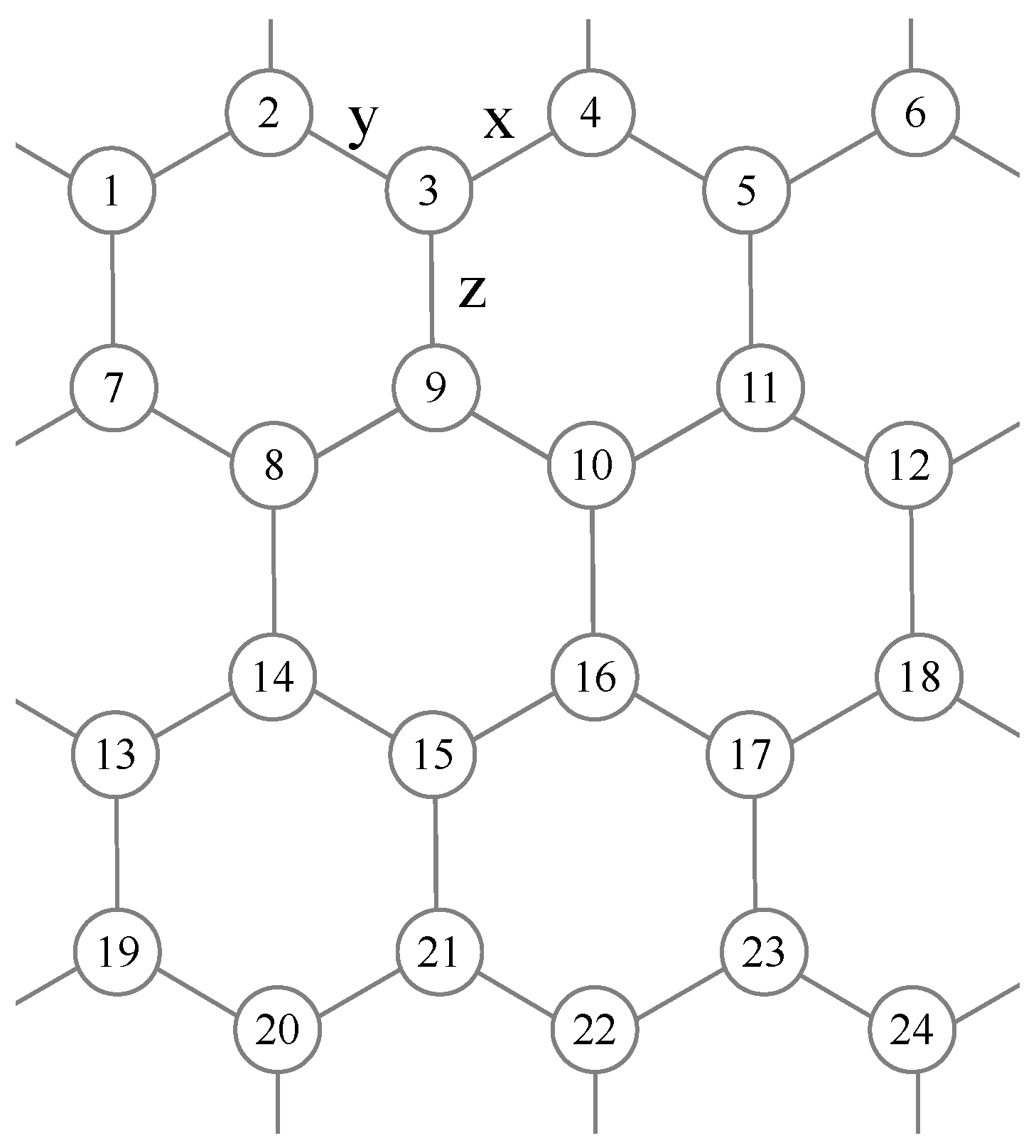
Figure 2.
The exact ground state energy of six sub-Hamiltonian demonstrate different behavior with coupling parameters.
Figure 2.
The exact ground state energy of six sub-Hamiltonian demonstrate different behavior with coupling parameters.
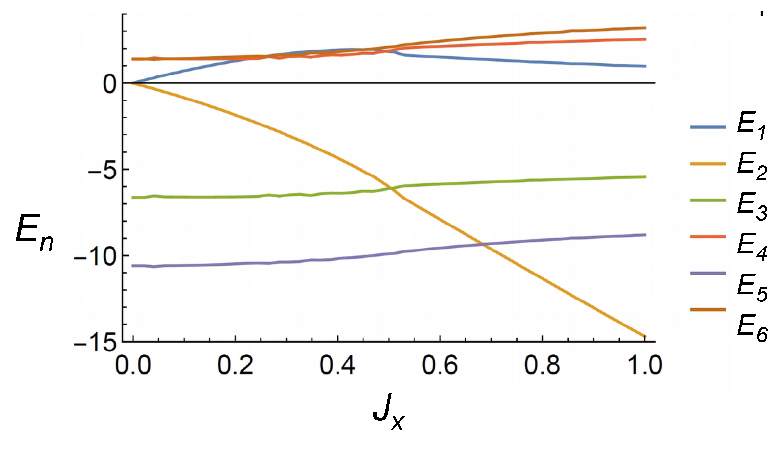
Figure 3.
(a) The pattern energy and with , (b) The pattern energy and with , (c) The pattern energy and with , (d) The pattern energy and with .
Figure 3.
(a) The pattern energy and with , (b) The pattern energy and with , (c) The pattern energy and with , (d) The pattern energy and with .
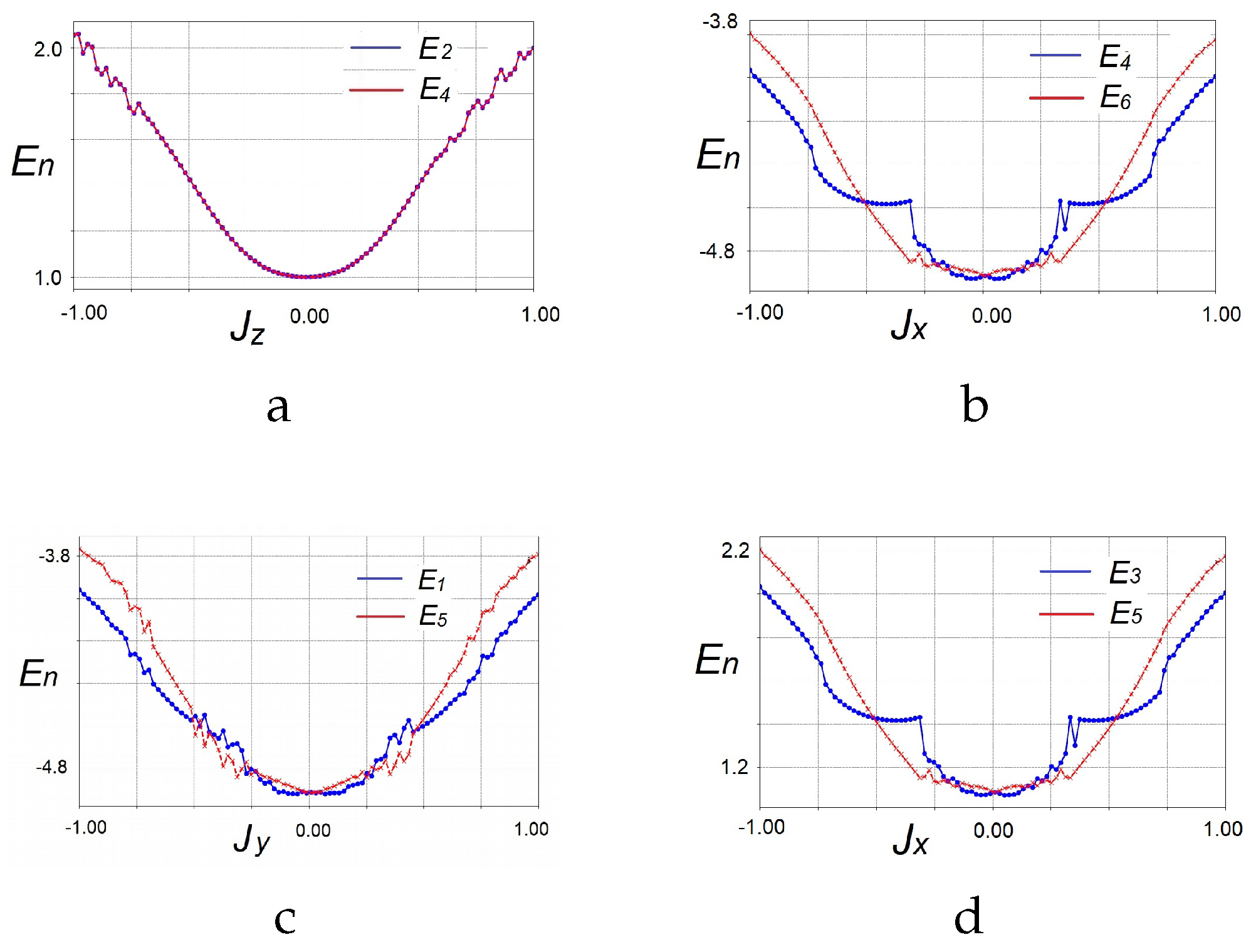
Figure 4.
The ground state energy varies with coupling parameters, for fixed momentum vectors, . (a) The gapped phase, ; (b) The gapless phase, .
Figure 4.
The ground state energy varies with coupling parameters, for fixed momentum vectors, . (a) The gapped phase, ; (b) The gapless phase, .
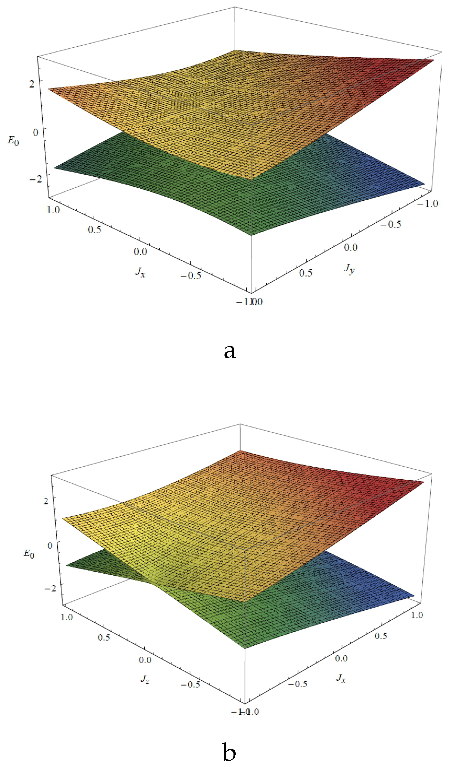
Figure 5.
(a) The coefficient vector at the ith site is illustrated by dyed rhombuses within one hexagon. (b) The red rhombus represents positive , and the unfilled rhombus represents negative . (c) The coefficient vector distribution around one hexagonal plaquette is represented by six dyed hexagons around the plaquette.
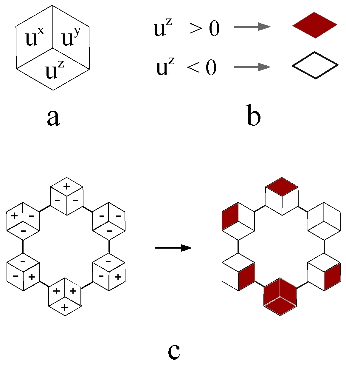
Figure 6.
The collective pattern with following parameters: . (a) ferromagnetic pattern, ; (b) anti-ferromagnetic pattern, ; (c) strip pattern, ; (d) dimer lattice pattern, .
Figure 6.
The collective pattern with following parameters: . (a) ferromagnetic pattern, ; (b) anti-ferromagnetic pattern, ; (c) strip pattern, ; (d) dimer lattice pattern, .
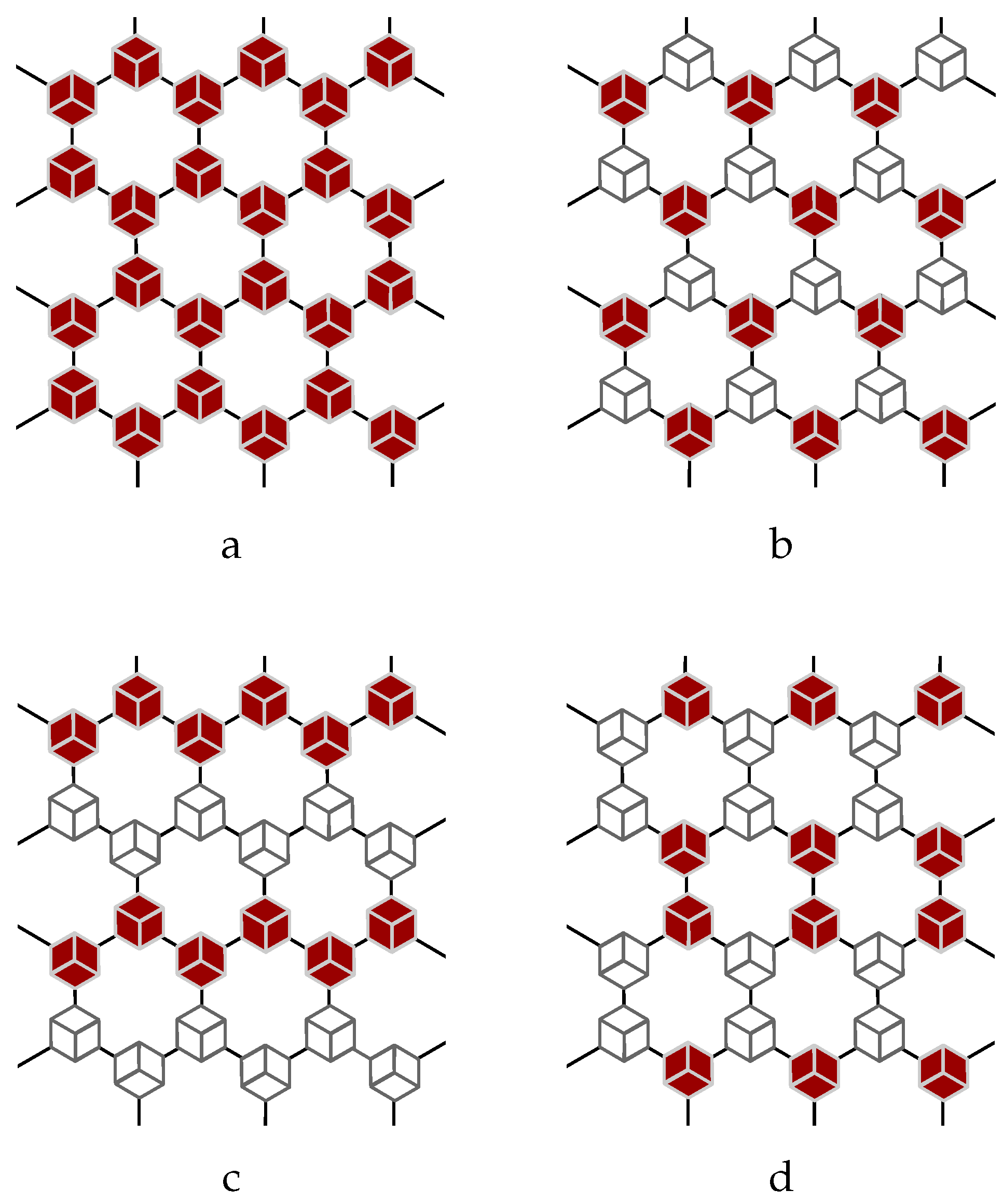
Figure 7.
The collective pattern of inhomogeneous vectors with following parameters: . (a) ferromagnetic pattern, ; (b) anti-ferromagnetic pattern, ; (c) strip pattern, ; (d) dimer lattice pattern, .
Figure 7.
The collective pattern of inhomogeneous vectors with following parameters: . (a) ferromagnetic pattern, ; (b) anti-ferromagnetic pattern, ; (c) strip pattern, ; (d) dimer lattice pattern, .
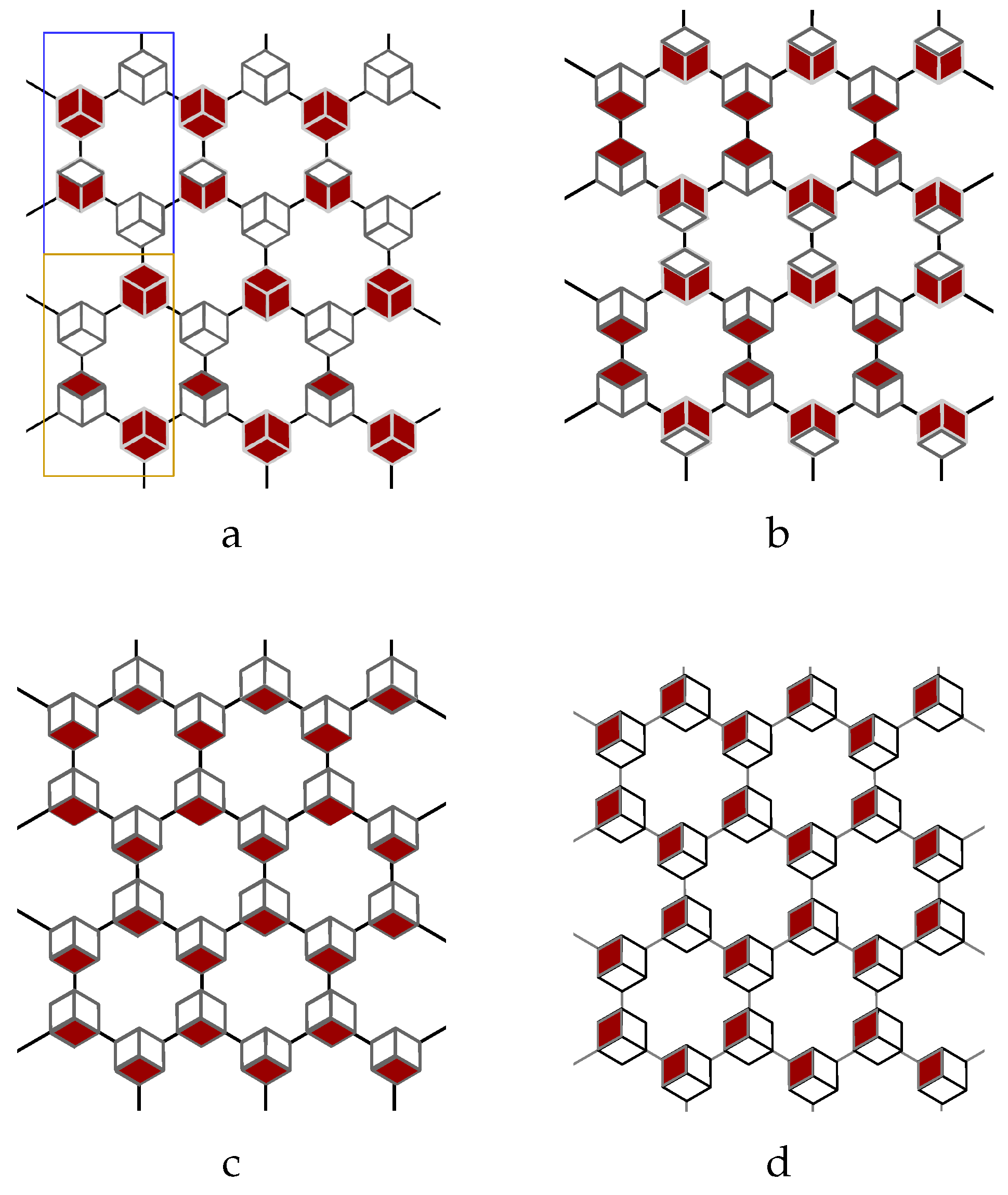
Figure 8.
The collective pattern of inhomogeneous vectors , . (a) ferromagnetic pattern lattice of four sites, ; (b) anti-ferromagnetic strip pattern, ; (c) plaquette pattern lattice, ; (d) plaquette dimer lattice, .
Figure 8.
The collective pattern of inhomogeneous vectors , . (a) ferromagnetic pattern lattice of four sites, ; (b) anti-ferromagnetic strip pattern, ; (c) plaquette pattern lattice, ; (d) plaquette dimer lattice, .
Disclaimer/Publisher’s Note: The statements, opinions and data contained in all publications are solely those of the individual author(s) and contributor(s) and not of MDPI and/or the editor(s). MDPI and/or the editor(s) disclaim responsibility for any injury to people or property resulting from any ideas, methods, instructions or products referred to in the content. |
© 2025 by the authors. Licensee MDPI, Basel, Switzerland. This article is an open access article distributed under the terms and conditions of the Creative Commons Attribution (CC BY) license (http://creativecommons.org/licenses/by/4.0/).
Copyright: This open access article is published under a Creative Commons CC BY 4.0 license, which permit the free download, distribution, and reuse, provided that the author and preprint are cited in any reuse.


