
Submitted:
08 October 2025
Posted:
08 October 2025
You are already at the latest version
Abstract
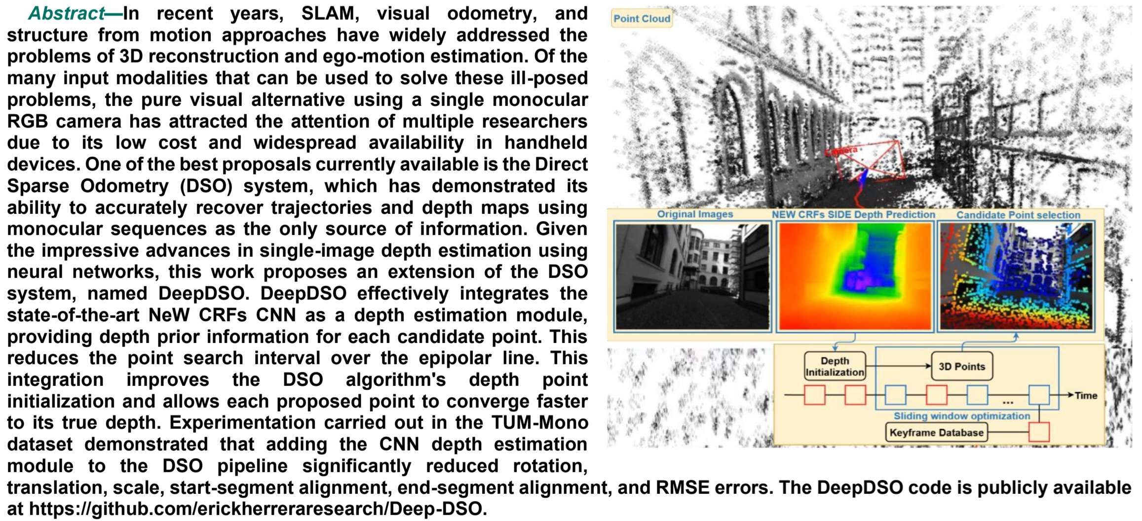
In recent years, SLAM, visual odometry, and structure from motion approaches have widely addressed the problems of 3D reconstruction and ego-motion estimation. Of the many input modalities that can be used to solve these ill-posed problems, the pure visual alternative using a single monocular RGB camera has attracted the attention of multiple researchers due to its low cost and widespread availability in handheld devices. One of the best proposals currently available is the Direct Sparse Odometry (DSO) system, which has demonstrated its ability to accurately recover trajectories and depth maps using monocular sequences as the only source of information. Given the impressive advances in single-image depth estimation using neural networks, this work proposes an extension of the DSO system, named DeepDSO. DeepDSO effectively integrates the state-of-the-art NeW CRFs CNN as a depth estimation module, providing depth prior information for each candidate point. This reduces the point search interval over the epipolar line. This integration improves the DSO algorithm's depth point initialization and allows each proposed point to converge faster to its true depth. Experimentation carried out in the TUM-Mono dataset demonstrated that adding the CNN depth estimation module to the DSO pipeline significantly reduced rotation, translation, scale, start-segment alignment, end-segment alignment, and RMSE errors. The DeepDSO code is publicly available at https://github.com/erickherreraresearch/Deep-DSO.
Keywords:
CNN direct sparse odometry
; monocular visual odometry
; monocular 3D reconstruction
; monocular ego-motion
; pure visual odometry
1. Introduction
Three-dimensional (3D) reconstruction is a challenging ill-posed problem that has been approached from multiple perspectives using various techniques to recover accurate geometric representations of real-world environments. Previously, researchers have proposed solving this problem using different sensors, such as lasers, infrared, radars, LIDARs, and cameras, as well as combinations of these sensors, including additional sensors like GPS and INS [1,2,3]. Due to notable improvements in computer vision over the past few decades, cameras have become a precise alternative for solving this problem. For 3D reconstruction, cameras can be used in stereo arrays that favor pixel triangulation, with additional active sensors such as infrared, active, and passive sensors, as well as RGB-D cameras. They can also be combined with inertial INS sensors or used alone [4]. The most interesting input modality for many researchers is the monocular RGB camera because of its low price, availability in most portable devices (like smartphones, tablets, and laptops), and independence from additional sensors (like infrared and laser sensors) that limit their application to large environments. Using a monocular camera as the sole source of information is convenient for many applications. However, it presents a more complex problem due to its lack of real-world prior information, such as depth or scale. Consequently, these methods typically require more effort and computational power. This is why all monocular, pure visual methods are scale-ambiguous—one of their main disadvantages compared to stereo, RGB-D, or RGB-INS methods—and it is considered one of the main sources of drift. Thus, the present work aims to address these issues by incorporating depth-prior information into a popular monocular RGB system.
The 3D reconstruction corresponds to the mapping process, which is typically an output of Simultaneous Localization and Mapping (SLAM), Visual Odometry (VO), and Structure from Motion (SFM). Multiple studies have contributed to improving this task because accurate mapping significantly improves the performance of SLAM, VO, and SFM systems, even for methods focused on ego-motion estimation. Most systems perform tracking from the geometry map, and it has been proven that it is easier to solve both tracking and mapping problems jointly [1,2]. As mentioned in the previous study [5], SLAM, VO, and SFM can be categorized into three groups: direct vs. indirect, dense vs. sparse, and classic vs. machine learning based. Indirect methods use preprocessing to extract visual features or optical flow from each image, considerably reducing the amount of information and allowing only sparse representations of the scene geometry to be obtained. In contrast, direct methods work directly with pixel intensities, allowing those systems to work with more image information, though this increases computation cost. Dense methods refer to algorithms that can recover most of the scene geometry, typically entire structures, objects, or surfaces. In contrast, sparse methods work with less information and can only recover sparse point clouds representing the environment. Finally, classic methods are those that depend entirely on mathematical, geometric, optimization, or probabilistic techniques without including machine learning (ML).
Consequently, ML methods correspond to proposals based on classic formulations that include ML techniques to improve the performance of each system from different perspectives. Recent advances in transformer-based architectures have revolutionized monocular depth estimation, with methods such as AdaBins [6] introducing adaptive binning strategies that leverage transformer encoders for global depth distribution analysis, and Dense Prediction Transformers (DPT) [7] demonstrating how vision transformers can provide fine-grained and globally coherent depth predictions. Additionally, reinforcement learning approaches have emerged as promising alternatives for visual odometry optimization, particularly in keyframe selection and feature management strategies that enhance traditional geometric methods [8]. Furthermore, multi-scale feature pyramid networks have been developed to improve monocular depth estimation through enhanced spatial and semantic information fusion across different resolution levels [9]. The taxonomy for SLAM, VO, and SFM methods suitable for the 3D reconstruction problem was proposed in [5] and is formed by combining the following classifications: Classic-Sparse-Indirect [10,11,12,13,14,15], Classic-Dense-Indirect [16,17], Classic-dense-direct [18,19,20], Classic-Sparse-Direct [21,22,23], Classic-Hybrid [24], ML-sparse-indirect [25,26,27], ML-dense-indirect [28,29,30,31,32], ML-dense-direct [33,34,35,36], ML + classic-sparse-direct [37,38,39,40], and ML-hybrid [41]. Additionally, previous work [42] evaluated different open-source methods across the entire taxonomy using an appropriate, large monocular benchmark [43] to identify significant differences in performance among taxonomy categories and their respective advantages and shortcomings. That study identified that sparse direct methods significantly outperform the other taxonomy categories. They achieved the lowest translation, rotation, and scale errors, as well as the lowest alignment root mean square error (RMSE) over the 50 sequences of the TUM-Mono dataset [43].
For these reasons, we selected the classic sparse direct method, DSO, one of the best classic methods available. We propose improving its depth map estimation module by integrating a Single Image Depth Estimation (SIDE) Neural Network (NN) module. The SIDE-NN module takes a single image as input and estimates the depth of each pixel, returning a numeric value for each pixel in a matrix. This improves the mapping capabilities of the DSO method and provides an accurate, scaled reconstruction1 using pixel-wise prior depth information estimated by the network. We selected the NeW CRFs SIDE technique because it was the state of the art in deep learning-based monocular depth estimation when the Deep-DSO method was developed. Experimental results show that DeepDSO outperformed its classic version in the rotation, translation, scale, and RMSE metrics by adding the NeW CRFs CNN module.
2.1. Related Works
Some proposals aim to improve the performance of sparse-direct methods by including a convolutional neural network (CNN) in their pipeline [37,38,39,40]. These methods have been integrated for disparity map estimation [44], replacing the depth estimation module with a CNN [45], joint depth, pose, and uncertainty estimation [38], depth mask estimation for moving object detection and segmentation [39], and pose transformation estimation [40]. Nevertheless, none of these studies have thoroughly investigated the potential of incorporating prior depth information to constrain the point search interval along the epipolar line, as outlined in [41], which was successfully applied to the SVO hybrid approach. Thus, the most similar related work to our approach is the CNN-SVO proposed in [41]. It took the SVO hybrid system and implemented a single-image depth estimation module to improve the depth estimation process. This process was originally computed incrementally using a Gaussian formulation for depth estimation and a Beta distribution for the inlier ratio. In the original SVO, the beta distribution parameters are calculated using incremental Bayesian updates and depth filters that converge when the variance is lower than a threshold. The CNN-SVO authors, however, proposed reducing the epipolar point search interval in the next frame by using the mean and variance of the inverse depth calculated from each pixel depth obtained by the SIDE-NN module. This allowed the SVO method to converge faster to true depth and achieve better scaling in the reconstruction. The open-source code CNN-DSO, published in [46], applied the same approach as CNN-SVO to the DSO algorithm using MonoDepth [47] SIDE depth estimation. However, the code did not correctly follow the proposal of [41], so it did not significantly outperform the DSO algorithm [42]. In contrast to this approach, we successively integrated Loo’s method [41] into the original DSO system. We also used the state-of-the-art SIDE-NN NeW CRFs, which significantly improved the performance of the sparse-direct method.
DeepDSO is distinguished from CNN-DSO by its successful integration, which extends beyond merely replacing the SIDE architecture through three critical contributions to the framework. First, we preserved the probabilistic Gaussian depth filtering framework of DSO by initializing the depth filter parameters with SIDE-NN predictions rather than replacing depth values directly. This maintains the capability of uncertainty-based inference. Second, we implemented epipolar search interval constraints that are theoretically grounded and operate through Bayesian inference, optimization regularization, and geometric filtering mechanisms. Third, we rigorously calibrated the variance coefficient through an experimental analysis to balance accommodating neural network predictions and preventing outliers. These integration mechanisms explain why the original DSO significantly outperformed CNN-DSO in rotation and alignment metrics despite the latter incorporating neural depth priors. Meanwhile, DeepDSO achieved substantial improvements, demonstrating that proper framework integration is as critical as depth estimation accuracy.
2. Materials and Methods
This study employed the DSO direct-sparse VO algorithm, the NeW CRFs depth estimation method, and an improved point map initialization technique. The selection of DSO as the foundational framework for this investigation was not arbitrary but rather derived from extensive prior research conducted by our team. In a comprehensive survey [5], we systematically analyzed 42 monocular 3D reconstruction methods across a complete taxonomy encompassing ten categories: classic and machine learning-based approaches combined with dense/sparse and direct/indirect/hybrid formulations. Subsequently, a rigorous comparative study [42] evaluated ten representative methods spanning this taxonomy on the TUM-Mono benchmark—the same dataset employed herein. Statistical analysis of over 1,000 runs per algorithm conclusively demonstrated that sparse-direct methods significantly outperformed all alternative taxonomic categories across multiple metrics (), with DSO achieving optimal performance. These prior investigations systematically explored the methodological variations and architectural alternatives that constitute conventional ablation studies, thereby establishing the empirical foundation for DeepDSO's design. Consequently, the present work focuses on demonstrating whether state-of-the-art neural depth estimation can further enhance the already superior DSO framework. Readers interested in detailed ablation analyses across taxonomic categories, comparison metrics, and hardware calibration are directed to references [5] and [42].
2.1. Review of the DSO Algorithm
Based on our previous comprehensive evaluation, DSO (Direct Sparse Odometry) has become a leading framework in the computer vision and robotics communities [5,42,48]. It particularly excels in monocular RGB visual odometry and 3D scene reconstruction tasks. Our previous comparative analysis examined ten state-of-the-art monocular RGB SLAM and visual odometry algorithms (see references [14,20,21,22,23,24,25,41,46,49,[50]) using the taxonomic framework established in [51]. This extensive evaluation conclusively demonstrated that sparse-direct methodologies substantially outperform alternative approaches in 3D reconstruction applications. For this reason, we selected DSO as the foundation for this investigation due to its open-source availability and superior performance within the sparse-direct category.
DSO's effectiveness stems from its sophisticated candidate point selection mechanism, which identifies feature points with optimal geometric properties for robust tracking and mapping. The algorithm implements a region-adaptive gradient threshold approach by partitioning input images into pixel blocks. For each block, the system computes a localized threshold value according to the formula , where represents the median absolute gradient magnitude across all pixels within that specific block and is a global constant parameter typically set to 7. This adaptive thresholding ensures consistent point distribution across varying illumination conditions and texture densities.
To maintain a uniform spatial distribution of the selected points throughout the image domain, the DSO subdivides each frame into blocks. Then, it selects the pixel with the maximum gradient magnitude within each block, provided that the magnitude exceeds the computed region-adaptive threshold. Blocks that fail to meet this criterion contribute no candidate points to the array , which effectively filters out low-textured regions.
DSO was inspired by works [20,52] as a direct method that maintains five to seven keyframes to form a sliding window. The parameters of this window are then optimized through photometric error minimization. In this way, in a sliding window, there exist keyframe poses and selected points , defining . The neighborhood pattern corresponded to a small spatial pattern of pixels surrounding each point , typically consisting of 8 pixels arranged in a specific configuration to provide sufficient photometric information while maintaining computational efficiency. The illumination parameters included the affine brightness transformation coefficients and , which modeled multiplicative and additive brightness changes between frames, respectively. Additionally, represents the exposure time for each frame, which was essential for photometric calibration when available. Then the photometric error that has to be minimized is defined as:
where was modeled as a heuristic weighting factor, and is the reprojected pixel for a point on the current image , which is calculated as:
where and are the projection and back-projection functions, and are the relative body rotation and translations between two frames obtained by the transformations and , and is the inverse depth of a point
On the other hand, the DSO front end is responsible for selecting sets of keyframes and points and that will be used for photometric error optimization. It also provides initialization parameters and decides which keyframes and points will be marginalized. Regarding keyframe management, when the DSO algorithm receives a new image, it estimates the initial pose by projecting all active points from the sliding window onto the image and performing the conventional direct alignment. A new keyframe is created for changes in the field of view, occlusions, disocclusions, and changes in exposure time. These changes are detected by computing the optical flow and the relative brightness factor. If a keyframe is required and the current frame meets the criteria, it will be added to the sliding window. The DSO sliding window is equivalent to a co-visibility graph. However, unlike ORB-SLAM, it is not persistent because old or redundant keyframes are marginalized outside the sliding window. Thus, it is constantly updated. The DSO algorithm maintains well-distributed keyframes across 3D space by marginalizing those that maximize the heuristically designed distance score shown in (3), that is computed based on the Euclidean distance, , between the keyframes and , and by setting a small constant, ε:
In DSO, sparse point management is achieved by heavily subsampling data across processed frames, which considerably reduces computation and redundant information. Unlike indirect methods, which use only a set of features for certain types of information, such as edges and corners, DSO can sample all available data. This allows for tracking in weakly textured or repetitive regions. As previously detailed, candidate point selection is performed by looking for high gradient points that are well distributed over the image. So the pixel with the highest gradient above the threshold is selected. This process is repeated twice, splitting the image into and blocks, to capture points with weaker gradients. Next, candidate points are tracked by performing a discrete search over the epipolar line and minimizing photometric error. Depth and variance are computed from the best match and used to constrain the search interval for the next frame. Our method contrasts with this approach in that we follow the proposal of [41], which established that the search interval for each point's depth could be constrained using a depth and variance obtained with a SIDE-NN depth estimator. This allows the depth to be initialized more effectively and converge more quickly, resulting in a better-scaled 3D reconstruction. Finally, candidate points are activated to replace old marginalized points, maintaining a uniform spatial distribution across the image.
2.2. Review of NeW CRFs Single Image Depth Estimation
Depth estimation is a widely studied discipline in the fields of robotics and computer vision. It can be addressed using systems such as lasers, radar, LIDAR, and cameras. A purely visual, monocular approach to this task is called SIDE. Many proposals have been made to solve this problem using traditional methods, machine learning (ML) methods, and combinations of both. Traditional approaches have explored estimating the depth of scene objects using features. However, studies such as [53] have shown that local features alone are insufficient to explain the depth of each pixel in an image. Later proposals worked with discriminatively trained Markov random fields (MRFs) and conditional random fields (CRFs), which effectively model the depth of each pixel and the relationship between pixels. This allows for better inference of depth maps from colors, pixel positions, occlusions, known object sizes, haze, defocus, and more. Another possibility is estimating the depth map of an image using neural networks. This has been addressed by regressing a continuous depth map from the image [47,54,55,56,57,58,59,60]. However, these systems are strictly dependent on training processes involving wide datasets with plenty of motion patterns and illumination changes. Since accurately recovering ground truth depth maps for training is difficult, other approaches addressed the possibility of adding auxiliary information to aid the neural network's training process. These approaches introduced additional sparse depth [61] or additional segmentation information [62,63]. These approaches tried to obtain the depth map of each image directly from image features, which makes it a difficult fitting problem requiring complex neural network structures.
In contrast, the Neural Window (NeW) conditional random field (CRF) method used in this study combines traditional and machine learning (ML) approaches. It includes an energy function with fully connected CRFs and optimizes it to produce an accurate depth map. Since CNNs have proven efficient for depth estimation tasks, some approaches have tried embedding them in neural networks. One approach uses CRFs to refine the CNN's output [64], while another integrates the CNN in its layers [65]. However, this implies high computational complexity because all the nodes must be connected within the entire graph in fully connected CRFs. Thus, the NeW CRF authors proposed splitting the graph into multiple sub-windows so that the nodes only need to be connected within each window, making CRFs feasible.
MRFS and CRFs are commonly used for heavy prediction tasks, such as depth estimation and semantic segmentation because they have been shown to effectively correct errors based on neighboring node information. Furthermore, fully connected CRFs are especially suitable for enlarging the receptive field [66]; thus, they were employed in the NeW CRFs method, in which the fully connected CRFs energy function was modeled as follows:
where represents the predicted depth value for a node, and represents the rest of the graph nodes. is the unary potential function calculated for each node by the predictor. is the pairwise potential function, modeled to connect pairs of nodes by:
with for and equal to zero otherwise. and represent the color and the position of a node, respectively. Following these principles, the unary potential is calculated by the distribution over the predicted values, while the pairwise potential depends on the colors and positions of pixel pairs:
where represents the input image and represents the probability distribution of the prediction. The pairwise potential is used to apply heuristic punishments based on position and color information. This encourages keeping distant colors and positions while punishing similar colors and adjacent pixels. As previously mentioned, this is calculated for each window instead of for the entire graph. To communicate information from non-overlapping windows, another energy function is calculated by successively shifting the windows by . To embed this formulation in a neural network decoder and enable the network to compute the potential functions, the unary and pairwise potentials were reformulated so that the network could directly obtain them as follows:
with representing the parameters of the unary network. represents each feature map, and is the weighting function. Then, for each node , all its pairwise potentials must be summed as:
where and are the weighting functions that the network must calculate. Finally, authors implemented a query vector and a key vector , which are combined for each patch window as matrices and . So, performing the dot product, the potential weight of any pair can be recovered for all the predicted values . Then, the relative position is introduced to solve (8) as follows:
in NeW CRFs, the neural reformulation of the energy function (equations 7-9) is employed, where the network learns the potential functions directly from the data. Specifically, the unary potential was computed by a convolutional network from image features, while the pairwise potential is calculated using the multi-head attention mechanism presented in equation (9). This neural formulation allows the CRF module to capture complex relationships between nodes while maintaining computational feasibility through the window-based approach, making it suitable for integration into the real-time DSO pipeline.
In brief, the new CRFs method was built using a bottom-up-top-down structure with four levels of neuronal CRF optimization. These levels are implemented as decoder modules. The encoders, which extract feature maps to input into the decoder CRFs, are based on the Swin-Transformer [67]. The NeW CRFs uses the Swin-Transformer architecture for its encoder because its hierarchical structure with shifted windows aligns naturally with the window-based FC-CRF approach, enabling efficient feature extraction at multiple scales while maintaining computational feasibility. Additionally, the multi-head self-attention mechanism inherent to transformers is well-suited for capturing complex pairwise relationships between image patches. This is essential for computing the pairwise potentials in the CRF energy function. Vision transformers have also demonstrated superior performance in aggregating local and global image information compared to traditional convolutional neural networks (CNNs), which is critical for depth estimation tasks requiring comprehensive scene understanding. Thus, the compatibility of the window size (7×7 patches) between the Swin-Transformer encoder and the FC-CRF decoder facilitated the seamless integration and end-to-end training of the entire architecture.
Figure 1 presents the structure of the Fully-connected CRFs (FC-CRFs) module and the network's bottom-up-top-down architecture.
2.3. An Improved Point-Depth Initialization for the DSO Algorithm
There are many ways to integrate the output of a SIDE-NN as prior information to improve SLAM or VO tasks. For example, one can replace the depth estimation module with a SIDE-NN module or use it to provide prior information; extract features or estimate the depth, posse, scale, or optical flow using an ML module; use an ML module for parameter estimation; or use semantic segmentation or dynamic object detection and segmentation to provide depth prior information and enhance depth estimation [5]. In a previous study [42], we provided experimental results showing that integrating a SIDE-NN to provide prior information significantly improves the performance of SLAM or VO systems [46,68]. In this work, we followed the strategy of [41] and adapted it to the DSO framework. Unlike feature-based methods that depend on feature matching, direct methods require the depths of the selected points to be recovered, enabling direct tracking. Therefore, accurate depth estimation is crucial. Furthermore, all monocular RGB SLAM and VO systems suffer from scale ambiguity issues. However, Loo’s method [41] proposed overcoming these issues by incorporating a point initialization strategy in which depth priors from a SIDE-NN module constrained the search interval for candidate points selected in keyframes. This strategy bounds the search interval from which the true depth of each point will be estimated.
As previously mentioned, the classic DSO method first searches for point candidates in subsequent frames using a discrete search over the epipolar line to minimize photometric error. For the best match, depth and associated variance are then computed using a probabilistic Gaussian framework that represents uncertainty in stereo-based depth estimation. DSO and many other direct methods randomly initialize these parameters. However, for candidate points selected in keyframes, the depth and variance can be accurately initialized using measurements from a SIDE-NN. This reduces uncertainty, shortens the search interval, and allows the probabilistic framework to converge faster to the true depth. Large uncertainty can lead to problems such as selecting erroneous correspondences along the epipolar line in neighboring frames and a large number of depth measurements that do not converge to their true depths. Providing depth prior information to limit the search interval reduces depth uncertainty. This improves initialization and allows new points to converge faster to their true depths in a scaled manner. The search interval focuses on values close to the depth estimated by the SIDE, allowing scaled reconstructions. Figure 2 depicts this effect.
The accuracy improvement achieved through the integration of NN depth priors operates through three complementary theoretical mechanisms. First, from a probabilistic perspective, the SIDE-NN priors transform the Bayesian inference process by providing an informative, rather than random, initialization of the inverse depth distribution parameters . These constrained priors reduce the hypothesis space to high-probability regions, enabling photometric optimization to converge to the global minimum instead of becoming trapped in local minima corresponding to erroneous correspondences along the epipolar line. Second, in regard to the non-convex optimization landscape, the depth priors act as a regularization mechanism that biases the highly non-convex photometric error function toward geometrically plausible solutions. By restricting the search interval to , the method eliminates large portions of the parameter space containing spurious local minima while preserving regions with true depth values. This balances photometric consistency with geometric plausibility. Third, from an epipolar geometry perspective, the NN-derived constraints establish geometric bounds that filter out inconsistent correspondences before they influence optimization. This geometric filtering is particularly effective in homogeneous or repetitive regions, where multiple candidate points exhibit similar photometric characteristics. It prevents the selection of false matches that would violate multi-view geometric consistency and propagate errors throughout the trajectory, despite low photometric error.
In this way, , candidate points in keyframes were initialized using depth estimates obtained from the SIDE-NN without removing DSO's depth estimation framework, which has proven its efficiency. Thus, we preserve the uncertainty-based inference capabilities inherited from [20,52]. For these keyframe candidate points, the randomly initialized inverse-depth value was replaced during initialization by the depth estimation at that pixel position obtained by the NeW CRFs method, . The depth variance was obtained by , where the coefficient 6 derives from established probabilistic depth filtering frameworks. Following the inverse depth parametrization introduced by [68], the search interval must encompass sufficient uncertainty while maintaining geometric constraints for reliable epipolar correspondence. The coefficient 6 corresponds to bound around the mean, which in Gaussian statistics captures approximately 99.7% of the probability mass. This formulation, originally established in [41] for the CNN-SVO system, balanced two competing requirements: preserving adequate search space to accommodate NN prediction noise while preventing excessive uncertainty that would permit outlier matches and scale drift. The denominator coefficient ensured that the depth search interval [ρᵢᵐⁱⁿ, ρᵢᵐᵃˣ] remained sufficiently constrained to facilitate rapid convergence to true depth values while maintaining the metric scale recovered by the SIDE-NN module. Preliminary sensitivity analysis on TUM-Mono sequences, presented in Table 1, confirmed that coefficients smaller than 6 overly restricted the search space, causing convergence failures, whereas coefficients larger than 6 introduced excessive uncertainty, degrading scale accuracy and increasing outlier inclusion.
Using the initialized parameters and , the depth search interval is defined as follows:
It is important to emphasize that SIDE-NN's depth predictions do not influence the gradient-based candidate point selection mechanism of DSO. According to the point management strategy described in [21], candidate points are chosen based solely on image gradient magnitude via region-adaptive thresholding, which operates independently of depth information. The NN depth estimation module is invoked only after candidate selection and only for keyframes. It provides depth priors solely to initialize the depth filter parameters and rather than modifying the selection process itself. This architectural separation ensures that potential biases in CNN predictions toward textured regions or object edges cannot alter the point distribution systematically since selection occurs before depth prediction. Consequently, DeepDSO preserves DSO's original gradient-driven spatial distribution of candidate points while benefiting from improved depth filter initialization. This reduces correspondence ambiguity and accelerates convergence to true depth values. Thus, depth prior information can guide the depth estimation process of the direct formulation by bounding the search interval for each point along the epipolar line of each new frame. Figure 3 shows the integration of the depth module in the DSO algorithm.
3. Results
The DSO and NeW CRF SIDE-NN integration was developed using the C++ and Python programming languages on the Ubuntu 18.04 operating system. For implementation and evaluation purposes, we selected affordable, readily available computer components to assemble a desktop based on the AMD Ryzen™ 7 3800X processor and NVIDIA GeForce RTX 3060 GPU. The technical specifications of the hardware used for evaluation are presented in Table 2.
In the previous study [42], ten open-source algorithms from each taxonomy category were tested using the monocular benchmark from [43]. This study demonstrated that sparse-direct methods significantly outperformed state-of-the-art methods. For this reason, this work is based on the classic sparse-direct method DSO due to its impressive results for monocular reconstruction. Thus, we compared the original DSO [21] and its ML update, CNN-DSO [42], to test whether the proposed method, DeepDSO, significantly outperforms the classic version and whether the newest NeW CRFs SIDE-NN significantly improves the performance of the sparse-direct method. DSO and CNN-DSO are both publicly available on GitHub as open-source code [46,70] and can be implemented with minimal requirements, including Pangolin V0.5 [71], OpenCV V3.4.16, TensorFlow V1.6.0, and the C++ version of MonoDepth [72], which is faster than its original Python implementation. Figure 4 shows examples of 3D reconstructions obtained using the DeepDSO algorithm. Figure 5 compares the three implementations running in the same sequences, both indoors and outdoors.
As Figure 5 shows, the DeepDSO algorithm considerably improves the mapping results. In the top row, which belongs to sequence_01 of the TUM-Mono dataset, the addition of the MonoDepth CNN to CNN-DSO reduces the mapping quality of DSO. This may be primarily because its integration did not follow the point search recommendations on the epipolar line provided in [41]. Additionally, the precision of the MonoDepth CNN is considerably lower than that of NeW CRFs, causing CNN-DSO to produce reconstructions with a large number of outliers. Additionally, DeepDSO recovers slightly denser and more precise reconstructions due to its improved depth initialization strategy for candidate points in keyframes, which allowed these points to converge faster to their true depth. Similarly, the bottom row of Figure 5 presents an outdoor example for , where DeepDSO again recovers slightly denser, more precise, and scaled reconstructions. In contrast, the previous neural proposal (CNN-DSO) recovers sparser reconstructions with a considerable number of outliers. MonoDepth CNN recovers depth maps of lower quality than NeW CRFs. Figure 6 presents this effect in more detail.
Figure 6 shows that the per-pixel depth estimation task has improved significantly in recent years. This improvement is evident in the newer SIDE NeW CRFs, which perform considerably better than MonoDepth, allowing for more precise, detailed, consistent, and reliable depth estimation. Figure 6b shows examples of MonoDepth SIDE, which performs poor depth estimation compared to the NeW CRFs, especially in the TUM-Mono dataset, which has different camera calibration than the Cityscapes dataset [73] (where MonoDepth was trained). Despite using the camera calibration compensation formula described in (11) [41], CNN-DSO remains incompatible with TUM-Mono 640×480 rectified images.
where represents the scaled estimated depth and is the focal length ratio for the current camera and the camera used in the training dataset. Additionally, the superior performance of NeW CRFs over previous SIDE proposals is justified in [66].
For the evaluation of visual SLAM and VO systems, many benchmarks have been collected and proposed in recent years, such as [43,73,74,75,76,77,78,79,80,81,82]. However, only a few of these are designed specifically for evaluating monocular RGB systems and were recorded using monocular cameras. Of these, we considered: The KITTI dataset [76], which contains 21 video sequences of a driving car; the EUROC-MAV dataset [77], which contains 11 inertial stereoscopic sequences of a flying quadcopter; the TUM-Mono dataset [43], which contains 50 sequences comprising indoor and outdoor examples with more than 190,000 frames and over 100 minutes of video; and the ICL-NUIM dataset [74], which comprises eight video sequences of two environments with their respective ray tracing. Among the datasets suitable for evaluating monocular RGB systems, the TUM-Mono dataset is the most complete. It is also the most compatible with sparse-direct systems because it provides full photometric calibration information for the cameras, which is useful for these systems.
This investigation focuses on reconstructing indoor and outdoor scenarios from handheld monocular sequences with loop-closure characteristics typical of pedestrian navigation. While established benchmarks such as KITTI (automotive driving), EuRoC (aerial navigation), and ICL-NUIM (synthetic environments) provide valuable evaluation frameworks, their motion patterns and environmental conditions fall outside our current scope. Therefore, the TUM-Mono dataset was selected as it specifically addresses handheld monocular sequences captured by walking persons in closed-loop trajectories. Future research will evaluate the approach on automotive and aerial benchmarks to assess generalizability across diverse motion patterns. This dataset enabled comprehensive evaluation of currently available monocular sparse-direct methods [21,22,83,84,85].
As previously mentioned, the performance of the monocular RGB method can be evaluated from different perspectives. For instance, scene geometry can be represented as structures, surfaces, or point clouds, which can be dense or sparse. Therefore, to make an accurate comparison, a good, defined ground truth is required. However, dense and accurate point clouds are difficult to obtain and are not included in existing benchmarks. As proposed in [43,83,84,86], the estimated trajectory is the best way to evaluate monocular RGB methods because most SLAM and VO approaches use a 3D reconstruction map to estimate camera pose from known features and points. Thus, a better-estimated trajectory implies an accurate map. The TUM-Mono benchmark provides the most complete set of metrics for evaluating pure visual systems. It evaluates each monocular system in multiple dimensions. In contrast, [86] only proposes two metrics: the absolute trajectory root mean square error (ATE) and the relative pose root mean square error (RPE) for evaluating pose and trajectory. The TUM-Mono benchmark considers the following metrics:
- Start and end segment alignment error. Each experimental trajectory was aligned with ground truth segments at both the start (first 10-20 seconds) and end (last 10-20 seconds) of each sequence, computing relative transformations through optimization:
- Translation, rotation and scale error: From these alignments, the accumulated drift was computed as , enabling the extraction of translation, rotation and scale error components across the complete trajectory.
- Translational RMSE: The TUM-Mono benchmark authors also established a metric that equally considers translational, rotational, and scale effects. This metric, named alignment error (), can be computed for the start and end segments. Furthermore, when calculated for the combined start and end segments, is equivalent to the translational RMSE:
We evaluated DeepDSO by comparing it with its classic version, DSO, and its neural update, CNN-DSO. As recommended in [21,43,83,84], we tested each algorithm in each of the 50 sequences of the TUM-Mono benchmark. We ran each algorithm ten times forward and ten times backward, for a total of 1,000 runs per algorithm and 3,000 runs for the entire evaluation. The results obtained in each run were stored in a file in the format , gathering each tracked position and its corresponding quaternion at each timestamp . We processed the trajectory results in MATLAB using the official scripts provided in the TUM-Mono benchmark. Figure 7 shows the cumulative translation, rotation, and scale errors obtained from 500 runs of each algorithm.
Figure 7 shows the accumulated error achieved by the algorithms over 500 runs. The y-axis represents the number of runs, and the x-axis represents the accumulated error achieved by each method after a certain number of runs. Thus, the best methods should be in the top-left corner of each diagram. Figure 4 shows that the DeepDSO algorithm outperforms the DSO and CNN-DSO methods in translation, rotation, and scale error metrics. This suggests that adding the NeW CRFs SIDE-NN module to the DSO framework improves its performance, achieving better-scaled reconstructions and recovering accurate trajectories and rotations. This is evident in the reduction of translation, rotation, and scale errors. However, the CNN-DSO update that included the MonoDepth SIDE module did not outperform the original DSO system, which gathered the largest amount of translation, rotation, and scale error. Additionally, Figure 8 presents the alignment error, which represents these effects in a single metric for the start and end segments.
As shown in Figure 8, DeepDSO performed better than the other methods for the alignment metrics at the start and end of the segments. This demonstrates that the addition of the NeW CFRs SIDE-NN module considerably improved the DSO system during the bootstrapping stage. This improvement is due to the NeW CFRs SIDE-NN's enhanced point initialization technique, which reduces the search interval over the epipolar line for the next frame, allowing the true depth to converge faster. Additionally, DeepDSO considerably reduced errors in the last segment. This means the improved depth initialization technique continued to contribute to better overall algorithm performance by reducing drift in each pose through more accurate depth and pose estimation. This is reflected in the final segment, which shows significant drift reduction. It should be noted that CNN-DSO exhibited a slight reduction in alignment error in the initial segment compared to DSO. This indicates that the addition of MonoDepth SIDE improves the initialization process for DSO. However, the considerable presence of outliers affected its performance throughout the rest of the trajectory, producing a higher end-segment alignment error. Next, we evaluated the effect of motion bias for the three algorithms by comparing the performance of each method when running forward and backward, and measuring their combined effect. Figure 9 presents motion bias for DeepDSO, DSO, and CNN-DSO.
The motion bias effect was defined in [43] as the behavior of a monocular SLAM or VO system in different environments and with different motion patterns. As Figure 9 shows, DeepDSO exhibits a lower motion bias effect than the other tested algorithms. This indicates more robust and reliable performance with different motion patterns and changes, such as fast movements, strong rotations, and textureless surfaces. This can be attributed to the addition of a SIDE-NN module, which allows the DSO system to recover better, scaled information of each environment. This effectively limits the introduction of outliers and noisy estimations, thereby improving DSO performance. Furthermore, as seen in Figure 9, DeepDSO achieves a lower root mean square error (RMSE) in the backward modality. This is considerably different from the original DSO, where system performance diminished in backward runs. Figure 10 depicts the total alignment error measured for each system run on the 50 sequences of the TUM-Mono benchmark in both forward and backward directions to facilitate visualization of each system's performance.
As Figure 10 shows, the DeepDSO method had the best performance of the three evaluated methods across the entire dataset. Although DeepDSO produced more errors when running forward (yellow, orange, and green pixels), it exhibited a considerable reduction in the frequency of backward errors, suggesting a more stable and reliable performance compared to DSO. DSO performs well forward but presents many backward failure cases, especially in sequences 13, 21, and 22. DeepDSO's performance is clearly better in these sequences but still presents minor issues in sequence 21. Conversely, CNN-DSO performed the worst, with many failure cases, particularly for backward runs. It failed for sequences 21 and 22.
For the sake of completeness, we performed a full statistical analysis of the results gathered by running the TUM-Mono benchmark on each algorithm, as proposed in [42]. We started the statistical analysis by collecting all the error metric information in a database. This database included the following dependent variables: translation error (), rotation error (), scale error (), start-segment alignment error (), end-segment alignment error (), and translational RMSE (). We considered the method and the forward and backward modalities as categorical variables. Next, we used Mahalanobis distances as a data-cleaning technique to remove outliers. A cut-off score of 22.45774 was set based on the chi-squared distribution for a 99.999% confidence interval. This allowed us to detect and remove 94 outlier observations, leaving a database of 2,906 observations. Then, we tested the normality and homogeneity assumptions for each dependent variable using Kolmogorov-Smirnov and Levene's tests. As an example, running the Kolmogorov-Smirnov test for translation error yielded p-values of for DeepDSO, DSO, and CNN-DSO, which make up the sample. Thus, the normality assumption was rejected. We also obtained a p-value of in the Levene test and rejected the homogeneity assumption. Similar results were found when evaluating the other dependent variables. Therefore, it was concluded that the sample was nonparametric. Thus, the Kruskal–Wallis test was selected as the general test, and the Wilcoxon signed-rank test was selected as the post hoc test to determine whether the observed differences in the evaluation were significant. Figure 11 and Table 3 present the results obtained by applying statistical analyses to each dependent variable.
.
As can be seen in Figure 11 and Table 3, all Kruskal-Wallis comparisons reached the significance level. Thus, a Wilcoxon signed-rank test was performed for each dependent variable to determine which paired comparisons were significant. DeepDSO significantly outperformed DSO and CNN-DSO in the translation error metric, achieving an average reduction of 0.32211 in translation error compared to its classic predecessor, while DSO significantly outperformed CNN-DSO. For the accumulated rotation error metric, DeepDSO significantly outperformed the DSO and CNN-DSO methods, achieving an average error reduction of 0.2519316 compared to the classic version. Again DSO significantly outperformed the CNN-DSO method in the rotation error metric. DeepDSO also outperformed DSO and CNN-DSO significantly in the scale error metric, achieving an error reduction of 0.37644 compared to DSO. Meanwhile, CNN-DSO significantly outperformed DSO in this metric. Regarding the start-segment alignment error metric, DeepDSO significantly outperformed DSO and CNN-DSO, achieving an error reduction of 0.002317049 compared to its classic version, while DSO performed significantly better than CNN-DSO. As expected, Figure 5's behavior was confirmed for the end-segment alignment error metric: DeepDSO significantly outperformed DSO and CNN-DSO with an error reduction of 0.002048155, and DSO again outperformed CNN-DSO. Finally, for the RMSE metric, which considers all the aforementioned rotation, translation, and scale effects for both the start and end segments, DeepDSO significantly outperformed DSO and CNN-DSO, achieving an RMSE reduction of 0.1335233 and 0.14514478 compared to DSO and CNN-DSO, respectively. It should be noted that DSO achieved a slightly lower RMSE average score than CNN-DSO, though the difference was not significant.
Finally, a temporal analysis of frame-wise scale error was conducted for sequences 02 and 29 of the TUM-Mono benchmark. The frame-wise scale factor was computed by comparing incremental displacements between consecutive frames in the estimated trajectory with the ground truth, according to the methodology proposed by [87]. Then, the cumulative scale drift was calculated as the sum of the frame-wise errors across the trajectory. This provides insight into long-term stability without loop closure constraints. This method of evaluating scale drift dynamics was suggested by [88]. Figure 12 shows the temporal evolution of the cumulative scale drift for DeepDSO, DSO, and CNN-DSO across both sequences. The results showed that DeepDSO had substantially lower cumulative drift than DSO and CNN-DSO throughout both trajectories. The final accumulated errors were X and Y for sequences 02 and 29 of the TUM-Mono dataset, respectively. DeepDSO notably exhibited stable scale estimation beyond frame 500, where traditional methods diverged. This sustained stability without loop closure demonstrates that the depth estimation module provides continuous scale correction throughout optimization, effectively mitigating the accumulation of prediction errors inherent to purely geometric approaches [89].
4. Discussion
The TUM-Mono benchmark results, ratified by statistical analysis, demonstrated that integrating the NeW CRFs SIDE-NN module into the DSO framework significantly improved performance across all evaluated metrics: translation, rotation, scale, alignment, and RMSE. This confirmed that neuronal depth estimation modules substantially enhanced classic VO and SLAM systems for monocular applications. The experimental evidence revealed that these improvements stemmed from two synergistic mechanisms operating simultaneously. First, accurate depth initialization accelerated convergence during the windowed photometric optimization process—DSO's direct analogue to traditional bundle adjustment. The substantially lower start-segment alignment errors achieved by DeepDSO (0.001659 versus 0.003976 for DSO) indicated that NN depth priors constrained the search space to geometrically plausible regions, enabling faster convergence to better local optima during bootstrapping. Second, geometric constraints filtered erroneous correspondences before they contaminated the optimization window, substantially reducing outlier propagation. This mechanism was confirmed through comparative analysis: CNN-DSO, despite incorporating MonoDepth depth priors, produced reconstructions with considerable outlier contamination (Figure 5 and Figure 6) and higher end-segment alignment errors (0.006651), whereas DeepDSO achieved 0.002171 through proper epipolar constraint integration with the more accurate NeW CRFs network. The motion bias analysis (Figure 9) further demonstrated enhanced system stability, with DeepDSO maintaining consistent performance across forward and backward trajectory execution. These complementary mechanisms—accelerated optimization convergence and geometric outlier filtering—jointly explained the observed performance gains.
The proposed architecture employed a unidirectional design in which the SIDE-NN provided depth priors without receiving feedback from the DSO's optimization results. This open-loop formulation was deliberate. Closed-loop systems that require online CNN fine-tuning would introduce prohibitive computational overhead. For example, gradient backpropagation adds per keyframe, whereas the current inference time is . Closed-loop systems would also introduce potential instabilities, where optimization failures could corrupt learned priors. Training the NeW CRFs with self-supervised photometric consistency and spatial smoothness losses [66] ensured geometric coherence compatible with the DSO's multi-view optimization objectives. The statistical significance of the performance improvements (Table 3, ) validated the effective utilization of priors without requiring bidirectional coupling. Previous implementations [46], inspired by [41], addressed similar integration challenges but proved ineffective. CNN-DSO was significantly outperformed by original DSO in rotation, translation, and alignment errors, only achieving marginal improvements in scale recovery. This demonstrated that incorporating depth priors without proper integration allowed noisy data inclusion, ultimately degrading system performance due to MonoDepth's limited accuracy on TUM-Mono sequences and inadequate epipolar constraint implementation. Conversely, DeepDSO's superior scale error performance confirmed that the SIDE-NN module effectively contributed to properly scaled reconstructions. Since DSO's sparse-direct formulation tracks and manages every point and keyframe based on depth information, improved initialization directly enhanced both tracking and mapping capabilities, as evidenced by significant reductions in translation and rotation errors.
It is worth mentioning that a crucial component that enabled the successful implementation of the SIDE-NN module in the DSO algorithm was the CRF-based depth estimation approach. Adopting the NeW CRFs architecture instead of traditional fully-connected CRFs offered significant computational advantages for real-time depth estimation. As demonstrated in [66], segmenting the input into non-overlapping windows and computing fully-connected CRFs within each window rather than across the entire image reduces the computational complexity from to , where represents the total number of patches and denotes the window size. The reduced computational burden enables integrating CRF optimization into the visual odometry pipeline without compromising real-time performance requirements while maintaining geometric constraints that pure regression-based depth networks lack.
This investigation focused on handheld monocular sequences acquired while pedestrians moved along closed-loop trajectories. The TUM-Mono benchmark provided a comprehensive evaluation framework for these sequences. However, extending this approach to substantially different domains, such as autonomous driving (KITTI benchmark) or UAV exploration, was beyond the scope of this study and represents a direction for future work. As with all purely monocular methods, scale ambiguity was an inherent limitation. Although the SIDE-NN integration mitigated this issue by providing depth priors, complete elimination was unattainable because performance depended on depth estimation accuracy. Advances in SIDE architectures would directly benefit visual odometry systems. Additionally, pure visual methods have well-known challenges with illumination variations, occlusions, and low-texture surfaces. Deep learning techniques for object detection and semantic segmentation could address these issues. Finally, considerable computational requirements complicated deployment on resource-constrained embedded devices, with the transformer-based NeW CRFs module contributing substantially to these demands through its multi-head attention mechanisms and window-based fully-connected CRF operations. Despite the demonstrated improvements, convergence issues inherent to the direct sparse DSO framework remained susceptible to occurrence, albeit at reduced frequencies. These included photometric error optimization convergence failures in textureless regions, depth estimation convergence difficulties under rapid motion patterns, pose estimation convergence challenges when incorporating distant keyframes, and the absence of loop closure capabilities that could lead to trajectory drift accumulation. Drift was particularly expected to occur during extended trajectory sequences, rapid motion transitions, prolonged exposure to textureless environments, and scenarios with frequent occlusions or significant illumination variations. While the NeW CRFs epipolar line constraints effectively reduced outlier inclusion and scale-related errors, the fundamental algorithmic characteristics of sparse direct methods preserved these convergence vulnerabilities. Comprehensive analysis of these convergence behaviors and robust mitigation strategies constitute essential directions for future investigations. Future research could explore lightweight closed-loop architectures enabling bidirectional information flow through adaptive mechanisms such as confidence-weighted prior integration or test-time optimization updates modulated by photometric convergence indicators. Such approaches could potentially enhance performance by leveraging geometric feedback while maintaining real-time capability, though careful analysis of coupling dynamics would be required to preserve system robustness.
Although NeW CRFs and MonoDepth were primarily employed, alternative depth estimation methods were evaluated during the 2023 development phase. At that time, DepthFormer [90] and PixelFormer [91] represented state-of-the-art, open-access SIDE architectures. However, these methods exhibited prohibitively long inference times, averaging 5.27 seconds per image, rendering them impractical for real-time operation. In contrast, NeW CRFs and MonoDepth achieved inference times below one second, reaching up to 10 frames per second. Consequently, only these two architectures were incorporated into this comparative analysis. While newer SIDE models have since emerged, their evaluation and integration into the DeepDSO framework remain subjects for future work. Figure 13 presents depth inference examples using DepthFormer, PixelFormer, and NeW CRFs.
Figure 13.
Examples of depth inferences obtained using different SIDE-NNs: (a) DepthFormer, (b) PixelFormer, and (c) NeW CRFs.
Figure 13.
Examples of depth inferences obtained using different SIDE-NNs: (a) DepthFormer, (b) PixelFormer, and (c) NeW CRFs.
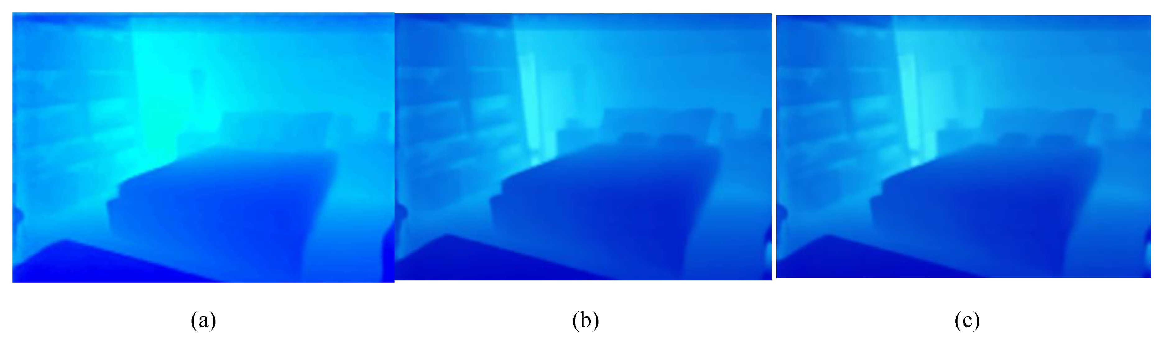
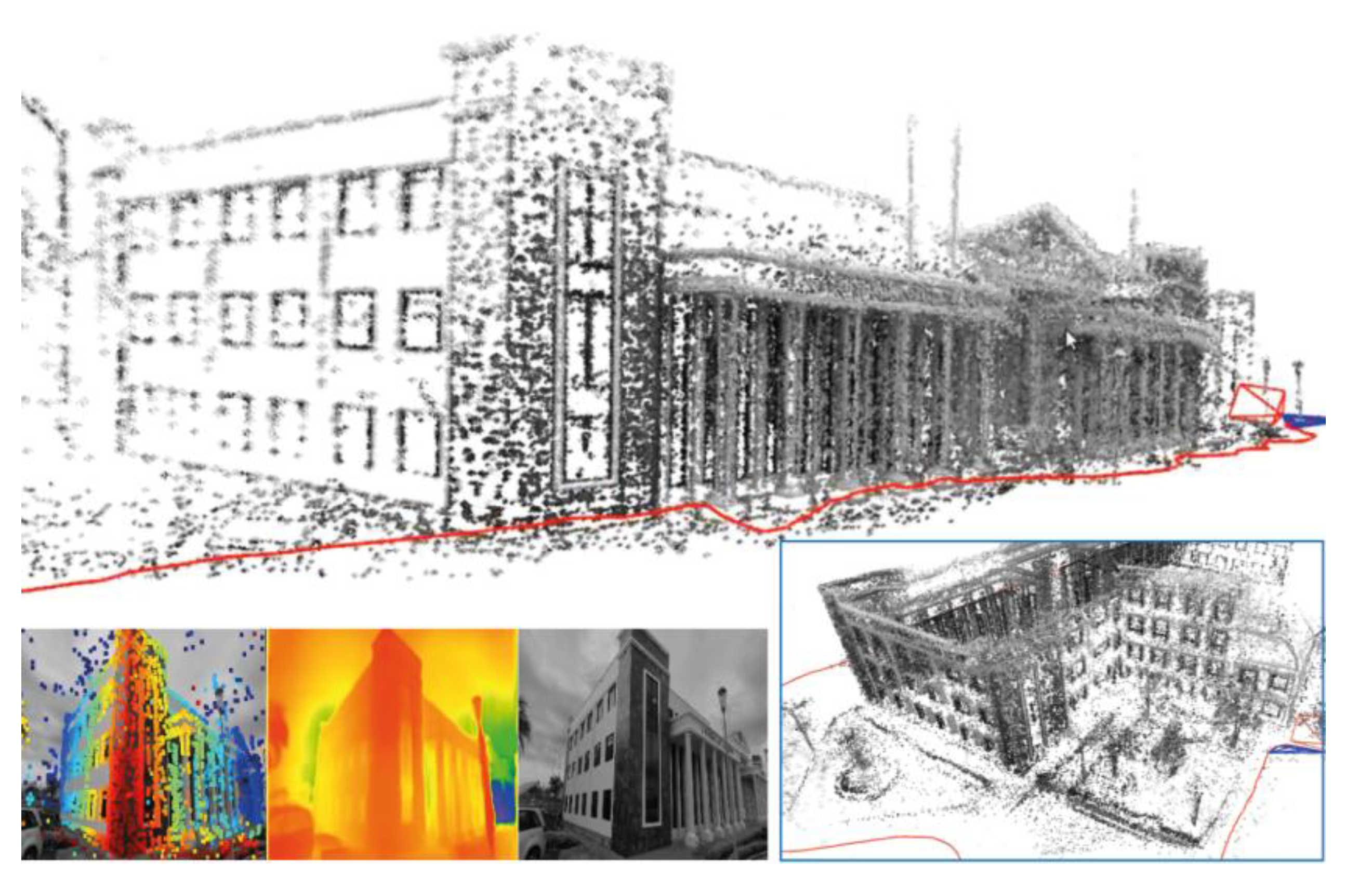
Figure 14.
3D map of the administrative building of Carchi State Polytechnic University captured with a standard smartphone camera (Xiaomi Redmi Note 10 Pro), without photometric calibration. As can be seen, DeepDSO can obtain 3D reconstructions and trajectories with non-specialized computer vision cameras without requiring exhaustive photometric calibration.
5. Conclusions
In this work, we propose an extension to the classic sparse direct VO system, DSO, by integrating the state-of-the-art NeW CRFs SIDE-NN as a depth estimation module. For candidate points selected in keyframes, this module provided depth prior information that reduced the point search interval over the epipolar line. This process enabled DSO to improve point initialization and allowed these points to converge faster to their true depth. Through over 3,000 runs on the publicly available TUM-Mono benchmark, we demonstrated that our proposal enhances the quality of 3D scene representation, enabling us to achieve slightly denser and scaled reconstructions. We evaluated DeepDSO's performance against the original DSO and a previous MonoDepth ML implementation. We found that DeepDSO significantly outperformed these methods in rotation, translation, scale, start-segment alignment error, end-segment alignment error, and RMSE metrics. This shows that our implementation helps obtain scaled 3D reconstructions and precise depth maps and trajectories.
Funding
This work was supported by SDAS Research Group (www.sdas-group.com).
Data Availability Statement
We made DeepDSO code publicly available in the GitHub repository: https://github.com/erickherreraresearch/Deep-DSO along with video samples of the execution DeepDSO algorithm for indoors and outdoors.
Acknowledgments
We acknowledge the Carchi State Polytechnic University of Ecuador for their support during the experimental stage of this research.
Conflicts of Interest
The authors declare no conflict of interest.
References
- Aqel, M.O.A.; Marhaban, M.H.; Saripan, M.I.; Ismail, N.B. Review of visual odometry: types, approaches, challenges, and applications. Springerplus 2016, 5, 1897. [Google Scholar] [CrossRef] [PubMed]
- Macario Barros, A.; Michel, M.; Moline, Y.; Corre, G.; Carrel, F. A Comprehensive Survey of Visual SLAM Algorithms. Robotics 2022, 11, 24. [Google Scholar] [CrossRef]
- Servières, M.; Renaudin, V.; Dupuis, A.; Antigny, N. Visual and Visual-Inertial SLAM: State of the Art, Classification, and Experimental Benchmarking. J. Sensors 2021, 2021, 1–26. [Google Scholar] [CrossRef]
- Zollhöfer, M.; Thies, J.; Garrido, P.; Bradley, D.; Beeler, T.; Pérez, P.; Stamminger, M.; Nießner, M.; Theobalt, C. State of the Art on Monocular 3D Face Reconstruction, Tracking, and Applications. Comput. Graph. Forum 2018, 37, 523–550. [Google Scholar] [CrossRef]
- Herrera-Granda, E.P.; Torres-Cantero, J.C.; Peluffo-Ordóñez, D.H. Monocular visual SLAM, visual odometry, and structure from motion methods applied to 3D reconstruction: A comprehensive survey. Heliyon 2024, 10, e37356. [Google Scholar] [CrossRef]
- S. Farooq Bhat, I. Alhashim, and P. Wonka, “AdaBins: Depth Estimation Using Adaptive Bins,” in 2021 IEEE/CVF Conference on Computer Vision and Pattern Recognition (CVPR), IEEE, Jun. 2021, pp. 4008–4017. [CrossRef]
- R. Ranftl, A. Bochkovskiy, and V. Koltun, “Vision Transformers for Dense Prediction,” Mar. 2021. [CrossRef]
- N. Messikommer, G. Cioffi, M. Gehrig, and D. Scaramuzza, “Reinforcement Learning Meets Visual Odometry,” Jul. 2024, [Online]. Available: http://arxiv.org/abs/2407.15626.
- H. Liu, D. D. Huang, and Z. Y. Geng, “Visual Odometry Algorithm Based on Deep Learning,” in 2021 6th International Conference on Image, Vision and Computing (ICIVC), IEEE, Jul. 2021, pp. 322–327. [CrossRef]
- H. Jin, P. Favaro, and S. Soatto, “Real-time 3D motion and structure of point features: a front-end system for vision-based control and interaction,” in Proceedings IEEE Conference on Computer Vision and Pattern Recognition. CVPR 2000 (Cat. No.PR00662), IEEE, 2000, pp. 778–779 vol.2. [CrossRef]
- Davison, A.J.; Reid, I.D.; Molton, N.D.; Stasse, O. MonoSLAM: Real-Time Single Camera SLAM. IEEE Trans. Pattern Anal. Mach. Intell. 2007, 29, 1052–1067. [Google Scholar] [CrossRef]
- R. Castle, “PTAM-GPL: Parallel Tracking and Mapping,” GitHub repository. [Online]. Available: https://github.com/Oxford-PTAM/PTAM-GPL.
- .Mur-Artal, R.; Montiel, J.M.M.; Tardos, J.D. ORB-SLAM: A Versatile and Accurate Monocular SLAM System. IEEE Trans. Robot. 2015, 31, 1147–1163. [Google Scholar] [CrossRef]
- Mur-Artal, R.; Tardos, J.D. ORB-SLAM2: An Open-Source SLAM System for Monocular, Stereo, and RGB-D Cameras. IEEE Trans. Robot. 2017, 33, 1255–1262. [Google Scholar] [CrossRef]
- Campos, C.; Elvira, R.; Rodriguez, J.J.G.; M. Montiel, J.M.; D. Tardos, J. ORB-SLAM3: An Accurate Open-Source Library for Visual, Visual–Inertial, and Multimap SLAM. IEEE Trans. Robot. 2021, 37, 1874–1890. [Google Scholar] [CrossRef]
- Valgaerts, L.; Bruhn, A.; Mainberger, M.; Weickert, J. Dense versus Sparse Approaches for Estimating the Fundamental Matrix. Int. J. Comput. Vis. 2011 962 2011, 96, 212–234. [Google Scholar] [CrossRef]
- R. Ranftl, V. Vineet, Q. Chen, and V. Koltun, “Dense Monocular Depth Estimation in Complex Dynamic Scenes,” in 2016 IEEE Conference on Computer Vision and Pattern Recognition (CVPR), IEEE, Jun. 2016, pp. 4058–4066. [CrossRef]
- J. Stühmer, S. Gumhold, and D. Cremers, “Real-Time Dense Geometry from a Handheld Camera,” in Lecture Notes in Computer Science (including subseries Lecture Notes in Artificial Intelligence and Lecture Notes in Bioinformatics), vol. 6376 LNCS, Springer, Berlin, Heidelberg, 2010, pp. 11–20. [CrossRef]
- M. Pizzoli, C. Forster, and D. Scaramuzza, “REMODE: Probabilistic, monocular dense reconstruction in real time,” in 2014 IEEE International Conference on Robotics and Automation (ICRA), IEEE, May 2014, pp. 2609–2616. [CrossRef]
- J. Engel, T. Schöps, and D. Cremers, “LSD-SLAM: Large-Scale Direct Monocular SLAM,” in Lecture Notes in Computer Science (including subseries Lecture Notes in Artificial Intelligence and Lecture Notes in Bioinformatics), vol. 8690 LNCS, no. PART 2, Springer Verlag, 2014, pp. 834–849. [CrossRef]
- Engel, J.; Koltun, V.; Cremers, D. Direct Sparse Odometry. IEEE Trans. Pattern Anal. Mach. Intell. 2018, 40, 611–625. [Google Scholar] [CrossRef] [PubMed]
- X. Gao, R. Wang, N. Demmel, and D. Cremers, “LDSO: Direct Sparse Odometry with Loop Closure,” in 2018 IEEE/RSJ International Conference on Intelligent Robots and Systems (IROS), IEEE, Oct. 2018, pp. 2198–2204. [CrossRef]
- Zubizarreta, J.; Aguinaga, I.; Montiel, J.M.M. Direct Sparse Mapping. IEEE Trans. Robot. 2020, 36, 1363–1370. [Google Scholar] [CrossRef]
- C. Forster, M. Pizzoli, and D. Scaramuzza, “SVO: Fast semi-direct monocular visual odometry,” in 2014 IEEE International Conference on Robotics and Automation (ICRA), IEEE, May 2014, pp. 15–22. [CrossRef]
- Bescos, B.; Facil, J.M.; Civera, J.; Neira, J. DynaSLAM: Tracking, Mapping, and Inpainting in Dynamic Scenes. IEEE Robot. Autom. Lett. 2018, 3, 4076–4083. [Google Scholar] [CrossRef]
- Steenbeek, “Sparse-to-Dense: Depth Prediction from Sparse Depth Samples and a Single Image,” GitHub repository. [Online]. Available: https://github.com/annesteenbeek/sparse-to-dense-ros.
- Sun, L.; Yin, W.; Xie, E.; Li, Z.; Sun, C.; Shen, C. Improving Monocular Visual Odometry Using Learned Depth. IEEE Trans. Robot. 2022, 38, 3173–3186. [Google Scholar] [CrossRef]
- B. Ummenhofer et al., “DeMoN: Depth and Motion Network for Learning Monocular Stereo,” in 2017 IEEE Conference on Computer Vision and Pattern Recognition (CVPR), IEEE, Jul. 2017, pp. 5622–5631. [CrossRef]
- Z. Teed and J. Deng, “DeepV2D: Video to Depth with Differentiable Structure from Motion,” Dec. 2018. [CrossRef]
- Z. Min and E. Dunn, “VOLDOR-SLAM: For the Times When Feature-Based or Direct Methods Are Not Good Enough,” CoRR, vol. abs/2104.0, Apr. 2021, [Online]. Available: https://arxiv.org/abs/2104.06800.
- Z. Teed and J. Deng, “DROID-SLAM: Deep Visual SLAM for Monocular, Stereo, and RGB-D Cameras,” in Advances in Neural Information Processing Systems, arXiv, 2021, pp. 16558–16569. doi: 10.48550/ARXIV.2108.10869. [CrossRef]
- C. Yang, Q. Chen, Y. Yang, J. Zhang, M. Wu, and K. Mei, “SDF-SLAM: A Deep Learning Based Highly Accurate SLAM Using Monocular Camera Aiming at Indoor Map Reconstruction With Semantic and Depth Fusion,” IEEE Access, vol. 10, pp. 10259–10272, 2022. [CrossRef]
- K. Tateno, F. K. Tateno, F. Tombari, I. Laina, and N. Navab, “CNN-SLAM: Real-Time Dense Monocular SLAM with Learned Depth Prediction,” in 2017 IEEE Conference on Computer Vision and Pattern Recognition (CVPR), IEEE, Jul. 2017, pp. 6565–6574. [CrossRef]
- T. Laidlow, J. T. Laidlow, J. Czarnowski, and S. Leutenegger, “DeepFusion: Real-Time Dense 3D Reconstruction for Monocular SLAM using Single-View Depth and Gradient Predictions,” in 2019 International Conference on Robotics and Automation (ICRA), IEEE, 19, pp. 4068–4074. 20 May. [CrossRef]
- M. Bloesch, J. M. Bloesch, J. Czarnowski, R. Clark, S. Leutenegger, and A. J. Davison, “CodeSLAM - Learning a Compact, Optimisable Representation for Dense Visual SLAM,” in 2018 IEEE/CVF Conference on Computer Vision and Pattern Recognition, IEEE, Jun. 2018, pp. 2560–2568. [CrossRef]
- Czarnowski, J.; Laidlow, T.; Clark, R.; Davison, A.J. DeepFactors: Real-Time Probabilistic Dense Monocular SLAM. IEEE Robot. Autom. Lett. 2020, 5, 721–728. [Google Scholar] [CrossRef]
- R. Cheng, C. Agia, D. Meger, and G. Dudek, “Depth Prediction for Monocular Direct Visual Odometry,” in 2020 17th Conference on Computer and Robot Vision (CRV), IEEE, May 2020, pp. 70–77. [CrossRef]
- N. Yang, L. von Stumberg, R. Wang, and D. Cremers, “D3VO: Deep Depth, Deep Pose and Deep Uncertainty for Monocular Visual Odometry,” in 2020 IEEE/CVF Conference on Computer Vision and Pattern Recognition (CVPR), IEEE, Jun. 2020, pp. 1278–1289. [CrossRef]
- F. Wimbauer, N. Yang, L. von Stumberg, N. Zeller, and D. Cremers, “MonoRec: Semi-Supervised Dense Reconstruction in Dynamic Environments from a Single Moving Camera,” in 2021 IEEE/CVF Conference on Computer Vision and Pattern Recognition (CVPR), IEEE, Jun. 2021, pp. 6108–6118. [CrossRef]
- Zhao, C.; Tang, Y.; Sun, Q.; Vasilakos, A. V. Deep Direct Visual Odometry. IEEE Trans. Intell. Transp. Syst. 2022, 23, 7733–7742. [Google Scholar] [CrossRef]
- S. Y. Loo, A. J. Amiri, S. Mashohor, S. H. Tang, and H. Zhang, “CNN-SVO: Improving the Mapping in Semi-Direct Visual Odometry Using Single-Image Depth Prediction,” in 2019 International Conference on Robotics and Automation (ICRA), IEEE, May 2019, pp. 5218–5223. [CrossRef]
- E. P. Herrera-Granda, J. C. Torres-Cantero, A. Rosales, and D. H. Peluffo-Ordóñez, “A Comparison of Monocular Visual SLAM and Visual Odometry Methods Applied to 3D Reconstruction,” Appl. Sci., vol. 13, no. 15, p. 8837, Jul. 2023. [CrossRef]
- J. Engel, V. Usenko, and D. Cremers, “A Photometrically Calibrated Benchmark For Monocular Visual Odometry,” Jul. 2016, Accessed: Jun. 11, 2021. [Online]. Available: http://arxiv.org/abs/1607.02555.
- S. Zhang, “DVSO: Deep Virtual Stereo Odometry,” GitHub repository. [Online]. Available: https://github.com/SenZHANG-GitHub/dvso.
- R. Cheng, “CNN-DVO,” 2020, McGill. [Online]. Available: http://www.cim.mcgill.ca/∼mrl/ran/crv2020.
- Muskie, “CNN-DSO: A combination of Direct Sparse Odometry and CNN Depth Prediction,” GitHub repository. [Online]. Available: https://github.com/muskie82/CNN-DSO.
- C. Godard, O. Mac Aodha, and G. J. Brostow, “Unsupervised Monocular Depth Estimation with Left-Right Consistency,” in 2017 IEEE Conference on Computer Vision and Pattern Recognition (CVPR), IEEE, Jul. 2017, pp. 6602–6611. [CrossRef]
- E. P. Herrera-Granda, Real-time monocular 3D reconstruction of scenarios using artificial intelligence techniques. 2024. [Online]. Available: https://hdl.handle.net/10481/90846.
- S. Wang, “DF-ORB-SLAM,” GitHub repository. [Online]. Available: https://github.com/834810269/DF-ORB-SLAM.
- J. Zubizarreta, I. Aguinaga, and J. M. M. Montiel, “Direct Sparse Mapping,” IEEE Trans. Robot., vol. 36, no. 4, pp. 1363–1370, 2020. [CrossRef]
- E. P. Herrera-Granda, J. C. Torres-Cantero, and D. H. Peluffo-Ordoñez, “Monocular Visual SLAM, Visual Odometry, and Structure from Motion Methods Applied to 3D Reconstruction: A Comprehensive Survey,” Heliyon - First Look, vol. 8, no. 23, pp. 1–61, 2023. [CrossRef]
- J. Engel, J. Sturm, and D. Cremers, “Semi-dense Visual Odometry for a Monocular Camera,” in 2013 IEEE International Conference on Computer Vision, IEEE, Dec. 2013, pp. 1449–1456. [CrossRef]
- Saxena, S. H. Chung, and A. Y. Ng, “Learning Depth from Single Monocular Images,” in Proceedings of the 18th International Conference on Neural Information Processing Systems, in NIPS’05. Cambridge, MA, USA: MIT Press, 2005, pp. 1161–1168.
- S. Aich, J. M. Uwabeza Vianney, M. Amirul Islam, and M. K. Bingbing Liu, “Bidirectional Attention Network for Monocular Depth Estimation,” in 2021 IEEE International Conference on Robotics and Automation (ICRA), 2021, pp. 11746–11752. [CrossRef]
- D. Eigen, C. Puhrsch, and R. Fergus, “Depth Map Prediction from a Single Image using a Multi-Scale Deep Network,” Adv. Neural Inf. Process. Syst., vol. 27, Jun. 2014, doi: 1406.2283v1.
- L. Huynh, P. Nguyen-Ha, J. Matas, E. Rahtu, and J. Heikkilä, “Guiding Monocular Depth Estimation Using Depth-Attention Volume,” in Computer Vision -- ECCV 2020, A. Vedaldi, H. Bischof, T. Brox, and J.-M. Frahm, Eds., Cham: Springer International Publishing, 2020, pp. 581–597.
- J. H. Lee, M.-K. Han, D. W. Ko, and I. H. Suh, “From Big to Small: Multi-Scale Local Planar Guidance for Monocular Depth Estimation,” 2019, arXiv.
- Lee, S.; Lee, J.; Kim, B.; Yi, E.; Kim, J. Patch-Wise Attention Network for Monocular Depth Estimation. Proc. AAAI Conf. Artif. Intell. 2021, 35, 1873–1881. [Google Scholar] [CrossRef]
- X. Qi, R. Liao, Z. Liu, R. Urtasun, and J. Jia, “GeoNet: Geometric Neural Network for Joint Depth and Surface Normal Estimation,” in 2018 IEEE/CVF Conference on Computer Vision and Pattern Recognition, 2018, pp. 283–291. [CrossRef]
- C. Godard, O. Mac Aodha, M. Firman, and G. Brostow, “Digging Into Self-Supervised Monocular Depth Estimation,” in 2019 IEEE/CVF International Conference on Computer Vision (ICCV), IEEE, Oct. 2019, pp. 3827–3837. [CrossRef]
- V. Guizilini, R. Ambruş, W. Burgard, and A. Gaidon, “Sparse Auxiliary Networks for Unified Monocular Depth Prediction and Completion,” in 2021 IEEE/CVF Conference on Computer Vision and Pattern Recognition (CVPR), 2021, pp. 11073–11083. [CrossRef]
- M. Ochs, A. Kretz, and R. Mester, “SDNet: Semantically Guided Depth Estimation Network,” in Pattern Recognition, G. A. Fink, S. Frintrop, and X. Jiang, Eds., Cham: Springer International Publishing, 2019, pp. 288–302.
- S. Qiao, Y. Zhu, H. Adam, A. Yuille, and L.-C. Chen, “ViP-DeepLab: Learning Visual Perception with Depth-aware Video Panoptic Segmentation,” in 2021 IEEE/CVF Conference on Computer Vision and Pattern Recognition (CVPR), 2021, pp. 3996–4007. [CrossRef]
- B. Li, C. Shen, Y. Dai, A. van den Hengel, and M. He, “Depth and surface normal estimation from monocular images using regression on deep features and hierarchical CRFs,” in 2015 IEEE Conference on Computer Vision and Pattern Recognition (CVPR), 2015, pp. 1119–1127. [CrossRef]
- Hua, Y.; Tian, H. Depth estimation with convolutional conditional random field network. Neurocomputing 2016, 214, 546–554. [Google Scholar] [CrossRef]
- W. Yuan, X. Gu, Z. Dai, S. Zhu, and P. Tan, “Neural Window Fully-connected CRFs for Monocular Depth Estimation,” in 2022 IEEE/CVF Conference on Computer Vision and Pattern Recognition (CVPR), 2022, pp. 3906–3915. [CrossRef]
- Z. Liu et al., “Swin Transformer: Hierarchical Vision Transformer using Shifted Windows,” in 2021 IEEE/CVF International Conference on Computer Vision (ICCV), 2021, pp. 9992–10002. [CrossRef]
- S. Y. Loo, “CNN-SVO,” GitHub repository. [Online]. Available: https://github.com/yan99033/CNN-SVO. [CrossRef]
- Civera, J.; Davison, A.J.; Montiel, J. Inverse Depth Parametrization for Monocular SLAM. IEEE Trans. Robot. 2008, 24, 932–945. [Google Scholar] [CrossRef]
- J. Engel, “DSO: Direct Sparse Odometry,” GitHub repository. [Online]. Available: https://github.com/JakobEngel/dso.
- S. Lovengrove, “Pangolin,” GitHub repository. [Online]. Available: https://github.com/stevenlovegrove/Pangolin/tree/v0.5.
- S.-Y. Loo, “MonoDepth-cpp,” GitHub repository. [Online]. Available: https://github.com/yan99033/monodepth-cpp.
- M. Cordts et al., “The Cityscapes Dataset for Semantic Urban Scene Understanding,” in 2016 IEEE Conference on Computer Vision and Pattern Recognition (CVPR), 2016, pp. 3213–3223. [CrossRef]
- Handa, T. Whelan, J. McDonald, and A. J. Davison, “A benchmark for RGB-D visual odometry, 3D reconstruction and SLAM,” in 2014 IEEE International Conference on Robotics and Automation (ICRA), IEEE, May 2014, pp. 1524–1531. [CrossRef]
- X. Huang et al., “The ApolloScape Dataset for Autonomous Driving,” in 2018 IEEE/CVF Conference on Computer Vision and Pattern Recognition Workshops (CVPRW), IEEE, Jun. 2018, pp. 1067–10676. [CrossRef]
- A. Geiger, P. Lenz, and R. Urtasun, “Are we ready for autonomous driving? The KITTI vision benchmark suite,” in 2012 IEEE Conference on Computer Vision and Pattern Recognition, IEEE, Jun. 2012, pp. 3354–3361. [CrossRef]
- Burri, M.; Nikolic, J.; Gohl, P.; Schneider, T.; Rehder, J.; Omari, S.; Achtelik, M.W.; Siegwart, R. The EuRoC micro aerial vehicle datasets. Int. J. Rob. Res. 2016, 35, 1157–1163. [Google Scholar] [CrossRef]
- D. J. Butler, J. Wulff, G. B. Stanley, and M. J. Black, “A Naturalistic Open Source Movie for Optical Flow Evaluation,” in European Conf. on Computer Vision (ECCV), A. Fitzgibbon et al. (Eds.), Ed., in Part IV, LNCS 7577. , Springer-Verlag, 2012, pp. 611–625. [CrossRef]
- A. R. Zamir, A. Sax, W. Shen, L. Guibas, J. Malik, and S. Savarese, “Taskonomy: Disentangling Task Transfer Learning,; in 2018 IEEE/CVF Conference on Computer Vision and Pattern Recognition, IEEE, Jun. 2018, pp. 3712–3722. doi: 10.1109/CVPR.2018.00391.
- Yin, W.; Liu, Y.; Shen, C. Virtual Normal: Enforcing Geometric Constraints for Accurate and Robust Depth Prediction. IEEE Trans. Pattern Anal. Mach. Intell. 2022, 44, 7282–7295. [Google Scholar] [CrossRef]
- J. Cho, D. Min, Y. Kim, and K. Sohn, “A Large RGB-D Dataset for Semi-supervised Monocular Depth Estimation,” Apr. 2019. [CrossRef]
- K. Xian et al., “Monocular Relative Depth Perception with Web Stereo Data Supervision,” in 2018 IEEE/CVF Conference on Computer Vision and Pattern Recognition, IEEE, Jun. 2018, pp. 311–320. [CrossRef]
- E. Mingachev et al., “Comparison of ROS-Based Monocular Visual SLAM Methods: DSO, LDSO, ORB-SLAM2 and DynaSLAM,” in Interactive Collaborative Robotics, A. Ronzhin, G. Rigoll, and R. Meshcheryakov, Eds., Cham: Springer International Publishing, 2020, pp. 222–233. [CrossRef]
- E. Mingachev, R. Lavrenov, E. Magid, and M. Svinin, “Comparative Analysis of Monocular SLAM Algorithms Using TUM and EuRoC Benchmarks,” in Smart Innovation, Systems and Technologies, vol. 187, Springer Science and Business Media Deutschland GmbH, 2021, pp. 343–355. [CrossRef]
- E. P. Herrera-Granda, “A Comparison of Monocular Visual SLAM and Visual Odometry Methods Applied to 3D Reconstruction,” GitHub repository. Accessed: Jun. 29, 2023. [Online]. Available: https://github.com/erickherreraresearch/MonocularPureVisualSLAMComparison.
- J. Sturm, N. Engelhard, F. Endres, W. Burgard, and D. Cremers, “A benchmark for the evaluation of RGB-D SLAM systems,” in 2012 IEEE/RSJ International Conference on Intelligent Robots and Systems, IEEE, Oct. 2012, pp. 573–580. [CrossRef]
- Z. Zhang, R. Zhao, E. Liu, K. Yan, and Y. Ma, “Scale Estimation and Correction of the Monocular Simultaneous Localization and Mapping (SLAM) Based on Fusion of 1D Laser Range Finder and Vision Data,” Sensors, vol. 18, no. 6, p. 1948, Jun. 2018. [CrossRef]
- E. Sucar and J.-B. Hayet, “Bayesian Scale Estimation for Monocular SLAM Based on Generic Object Detection for Correcting Scale Drift,” Nov. 2017, [Online]. Available: http://arxiv.org/abs/1711.02768.
- H. Strasdat, J. M. M. Montiel, and A. Davison, “Scale Drift-Aware Large Scale Monocular SLAM,” in Robotics: Science and Systems VI, Robotics: Science and Systems Foundation, Jun. 2010, pp. 73–80. [CrossRef]
- Agarwal and C. Arora, “Depthformer : Multiscale Vision Transformer For Monocular Depth Estimation With Local Global Information Fusion,” Jul. 2022, [Online]. Available: http://arxiv.org/abs/2207.04535.
- Agarwal and C. Arora, “Attention Attention Everywhere: Monocular Depth Prediction with Skip Attention,” Oct. 2022, [Online]. Available: http://arxiv.org/abs/2210.09071.
| 1 | Scaled reconstruction addresses the inherent scale ambiguity problem in purely monocular methods, which can recover accurate scene geometry but at arbitrary scales unrelated to real-world dimensions. The SIDE-NN module provides pixel-wise depth priors that enable more accurate scale recovery compared to classical approaches. |
Figure 1.
Diagram of the NeW CRFs' bottom-up-top-down NN architecture and its FC-CRFs module. represents the encoder’s output feature map; represents the upper-level prediction; and and represent the unary and pairwise potentials, respectively. The dashed lines show the decoder's FC-CRFs module, which builds a multi-head energy function from the upper-level predictions and the feature map to improve the prediction. Inspired by the article of [66].
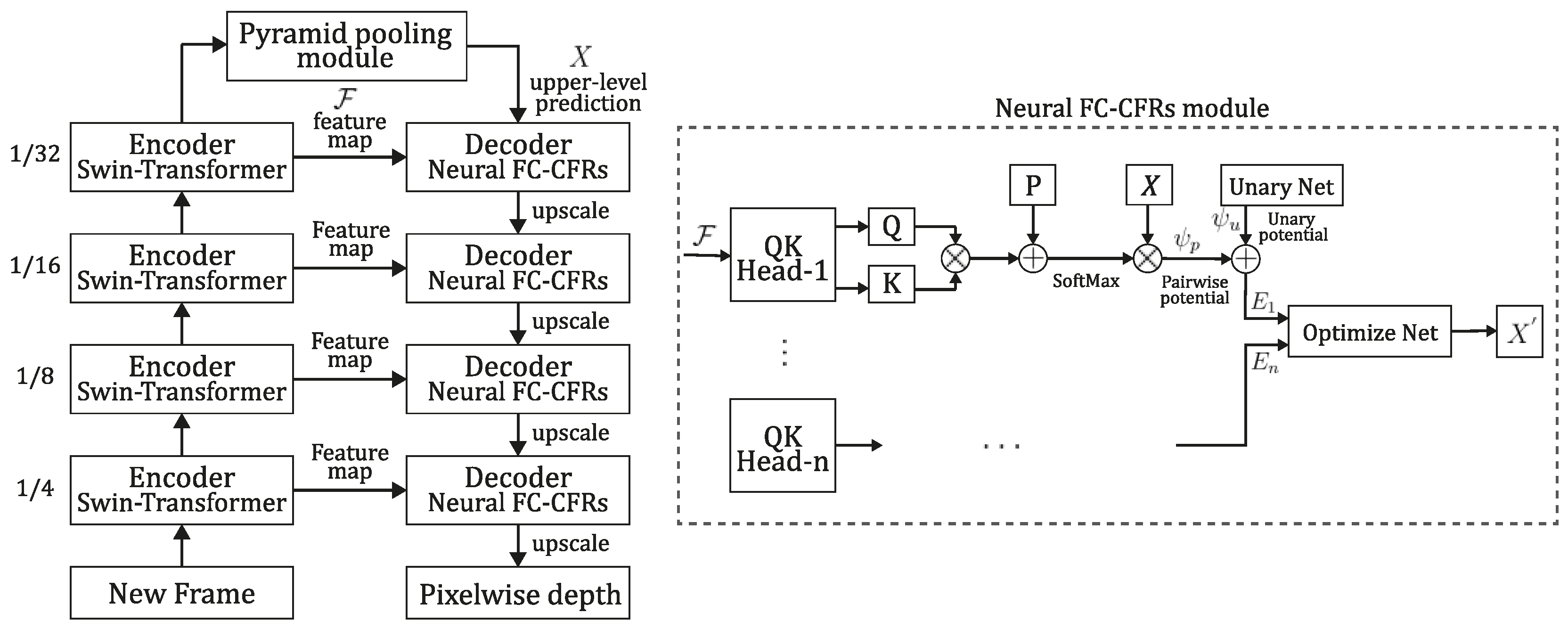
Figure 2.
Map point initialization strategy. The DSO searching interval along the epipolar line is improved by introducing prior information as depth and variance estimated using the SIDE-NN module. Figure (a) shows the DSO search interval without incorporating depth prior information. As shown in (b), the epipolar search interval in the next frame is reduced, enabling each point to converge to its scaled true depth while excluding similar points from the search interval.
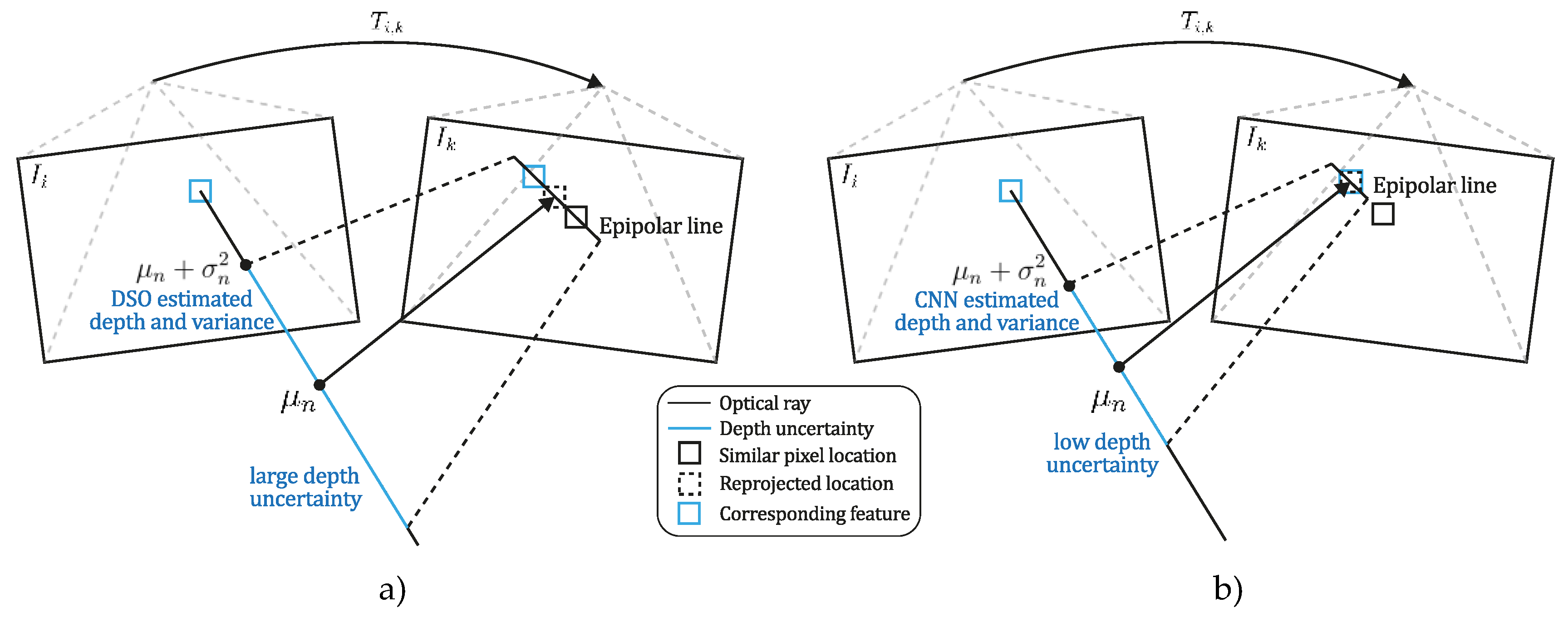
Figure 3.
Diagram of DeepDSO algorithm. Integrating the NeW CRFs SIDE-NN module in the DSO method.
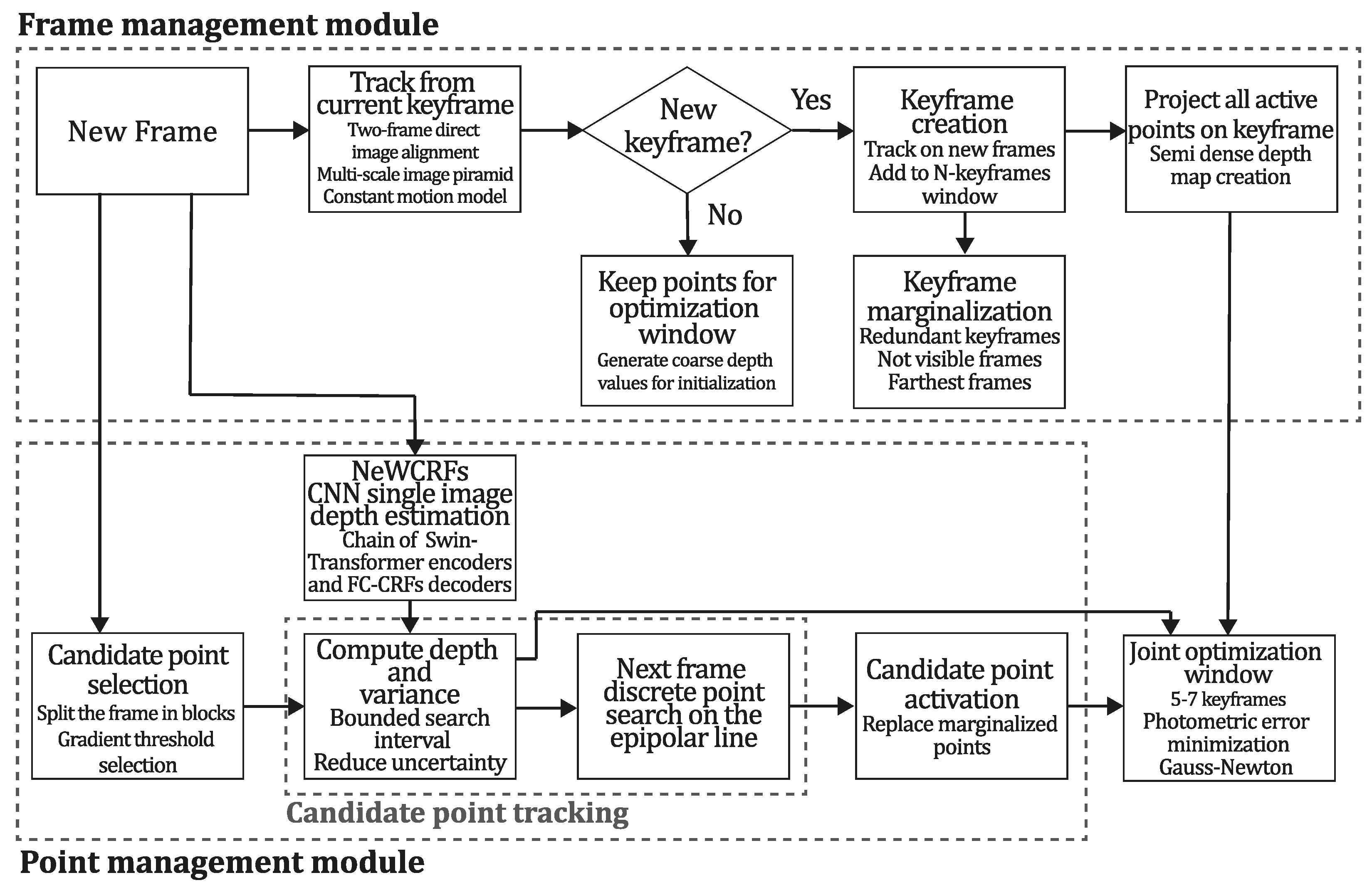
Figure 4.
Depth maps obtained with the DeepDSO method. Examples were obtained running the algorithm on the sequences a) 01, b) 20, c) 25, d) 29, e) 38, and f) 40 of the TUM-Mono dataset.
Figure 4.
Depth maps obtained with the DeepDSO method. Examples were obtained running the algorithm on the sequences a) 01, b) 20, c) 25, d) 29, e) 38, and f) 40 of the TUM-Mono dataset.
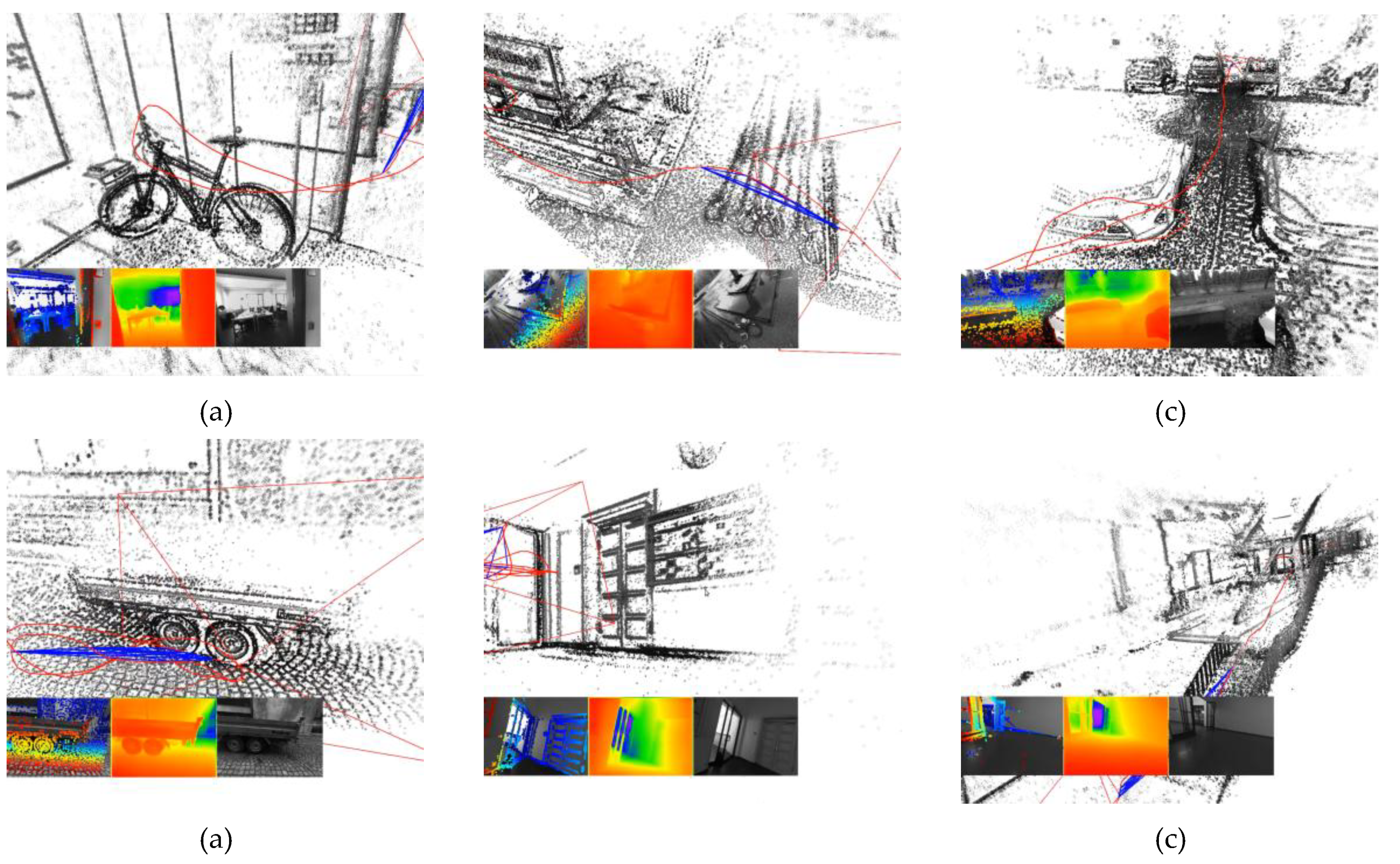
Figure 5.
Example reconstructions obtained using the evaluation algorithms. (a) represents the input image, and the geometry representations correspond to the (b) DSO, (c) CNN-DSO, and (d) DeepDSO methods. The top row shows indoor examples and the bottom row shows outdoor examples obtained using sequences 01 and 29 of the TUM-Mono dataset [43].
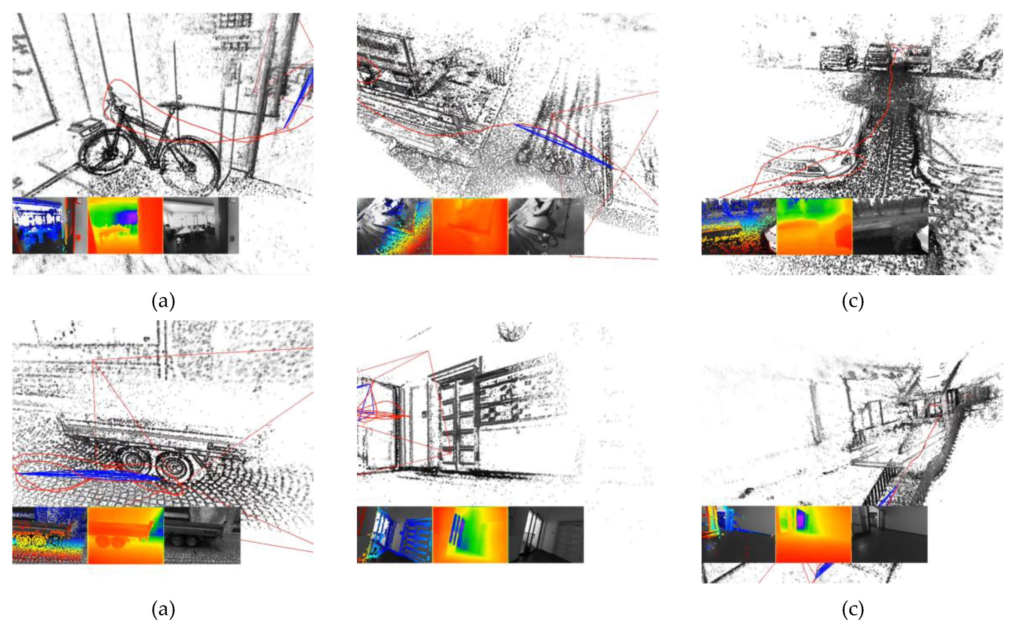
Figure 6.
Examples of the per-pixel depths recovered by the two SIDE modules that were tested. (a) shows the input image, (b) shows the output of MonoDepth, and (c) shows the output of the NeW CRFs. .
Figure 6.
Examples of the per-pixel depths recovered by the two SIDE modules that were tested. (a) shows the input image, (b) shows the output of MonoDepth, and (c) shows the output of the NeW CRFs. .
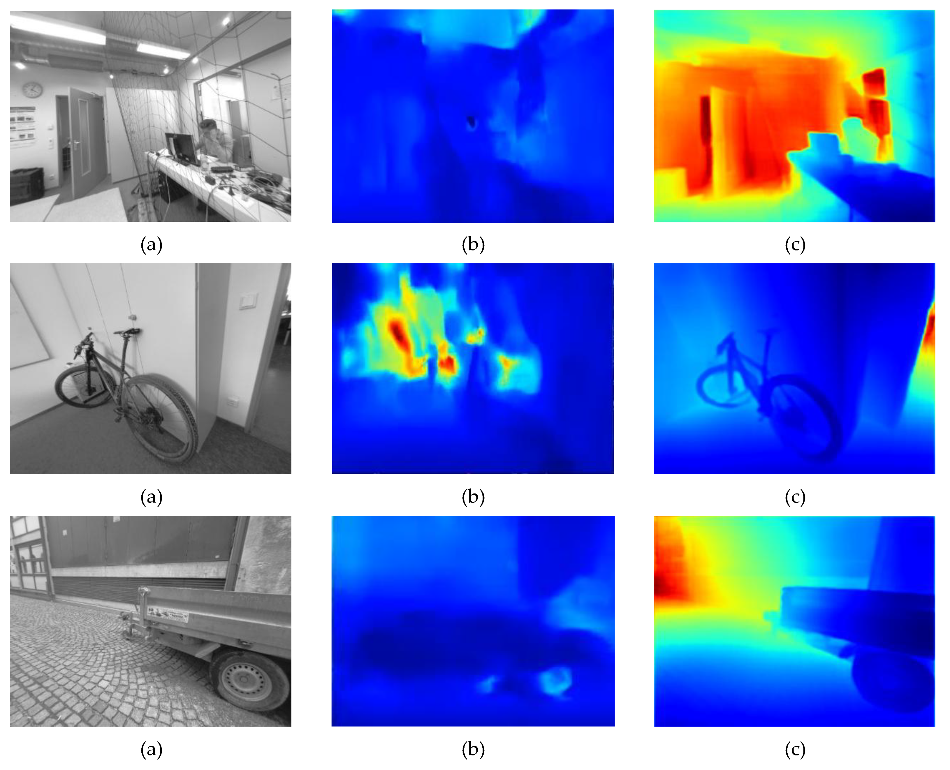
Figure 7.
Translation , rotation , and scale accumulated errors for the DeepDSO, DSO, and CNN-DSO algorithms evaluated algorithms.
Figure 7.
Translation , rotation , and scale accumulated errors for the DeepDSO, DSO, and CNN-DSO algorithms evaluated algorithms.
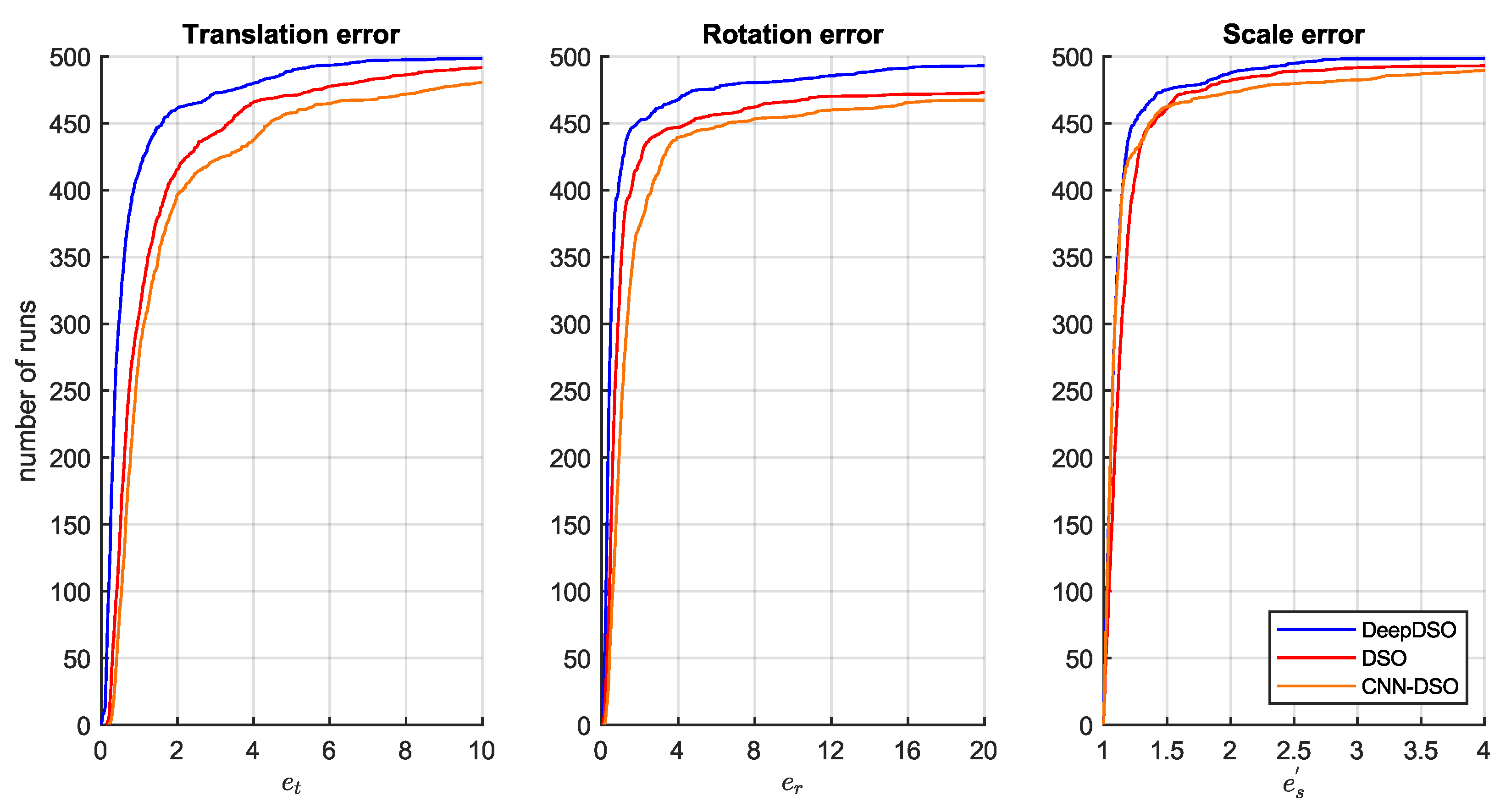
Figure 8.
Start- and end-segment alignment error, corresponding to the RMSE of the alignment error when compared with the start- and end-segment ground truth.
Figure 8.
Start- and end-segment alignment error, corresponding to the RMSE of the alignment error when compared with the start- and end-segment ground truth.
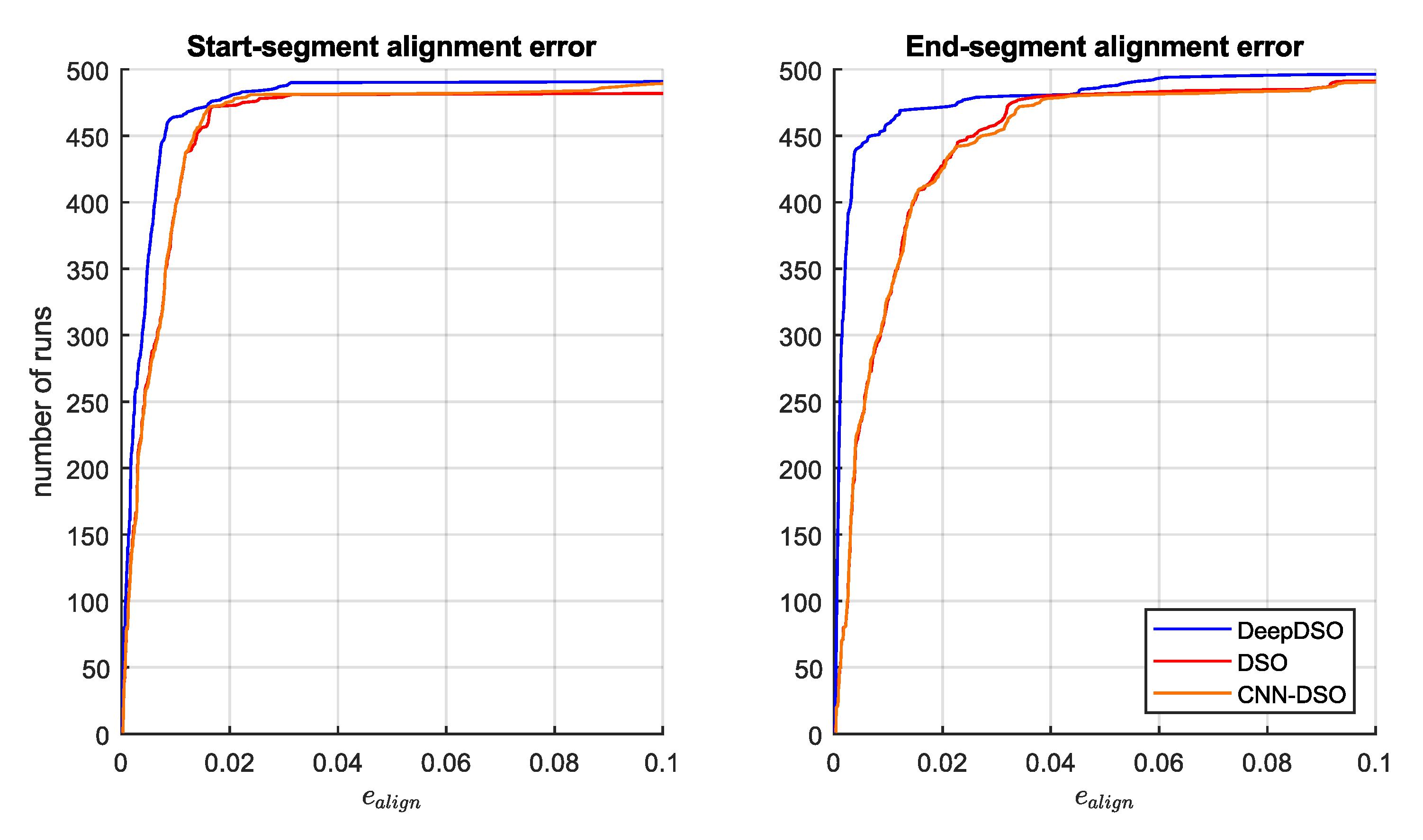
Figure 9.
Dataset motion bias for each method. They were evaluated by running all sequences forwards and backward, as well as their combination (bold).
Figure 9.
Dataset motion bias for each method. They were evaluated by running all sequences forwards and backward, as well as their combination (bold).
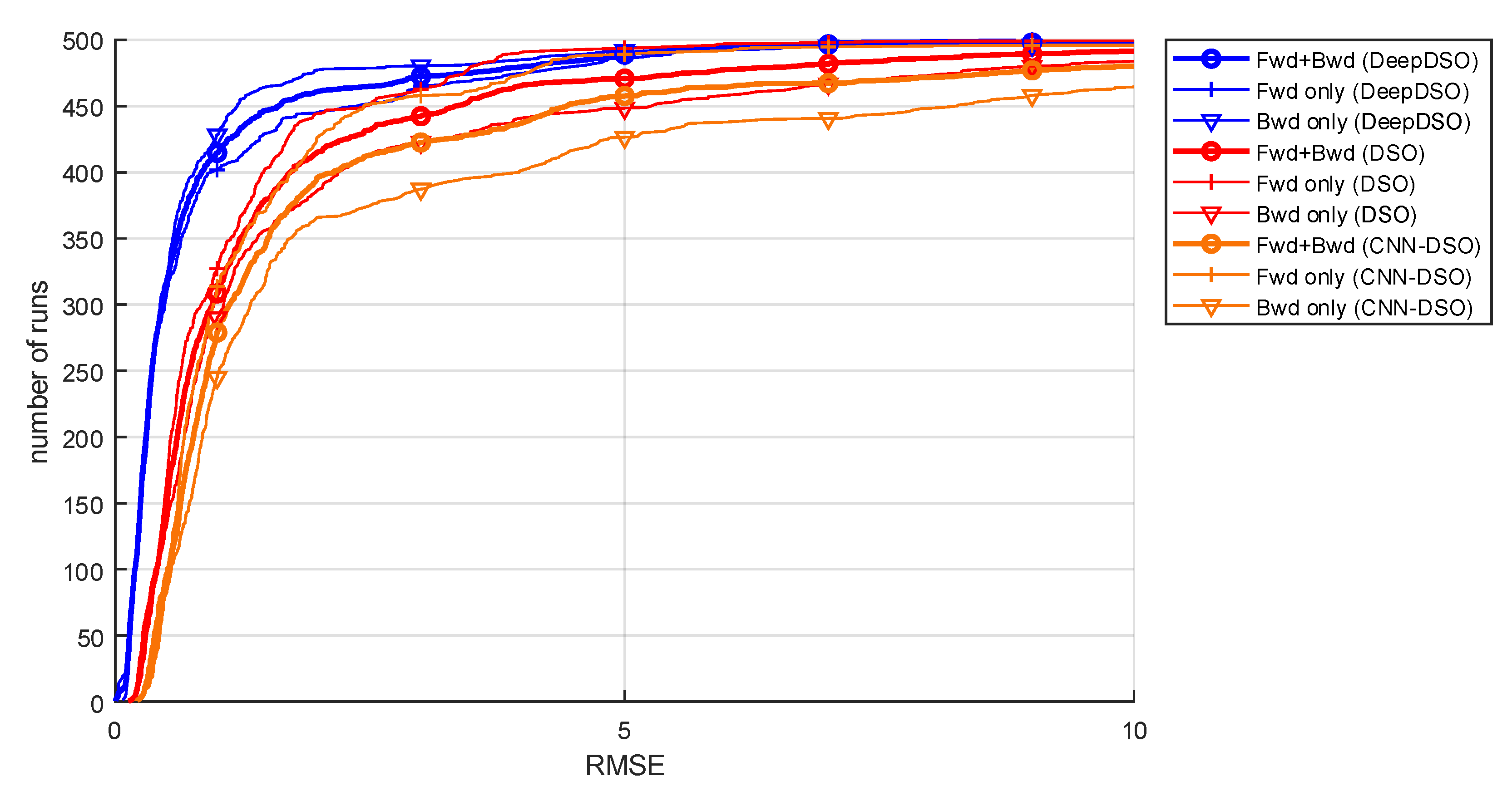
Figure 10.
Color-coded alignment error for each algorithm in the TUM-mono dataset.
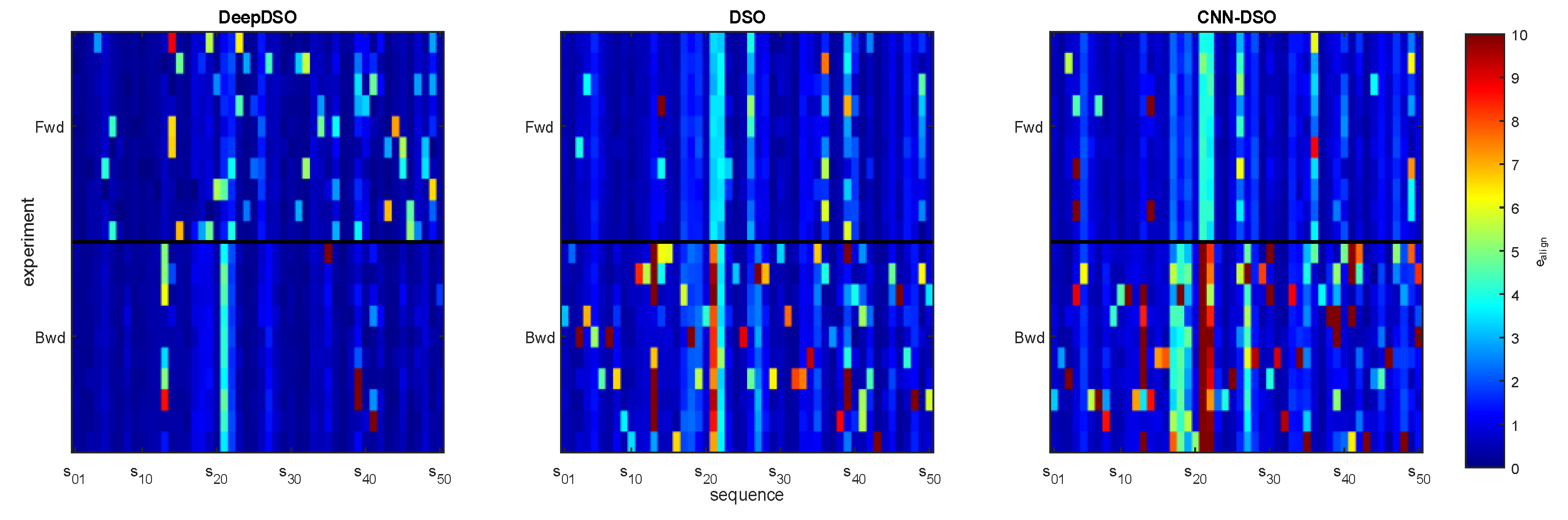
Figure 11.
Box plots, error bars, and Kruskal-Wallis comparisons for the medians of the cumulative errors collected after 1000 runs of each algorithm, (a) translation error, (b) rotation error, and (c) scale error, (d) only start-segment alignment error, (e) only end-segment alignment error, (f) RMSE for combined effect on start and end segments.

Figure 12.
Temporal evolution of cumulative scale drift on TUM-Mono sequences: (a) sequence 02 (650 frames) and (b) sequence 29 (1900 frames).
Figure 12.
Temporal evolution of cumulative scale drift on TUM-Mono sequences: (a) sequence 02 (650 frames) and (b) sequence 29 (1900 frames).
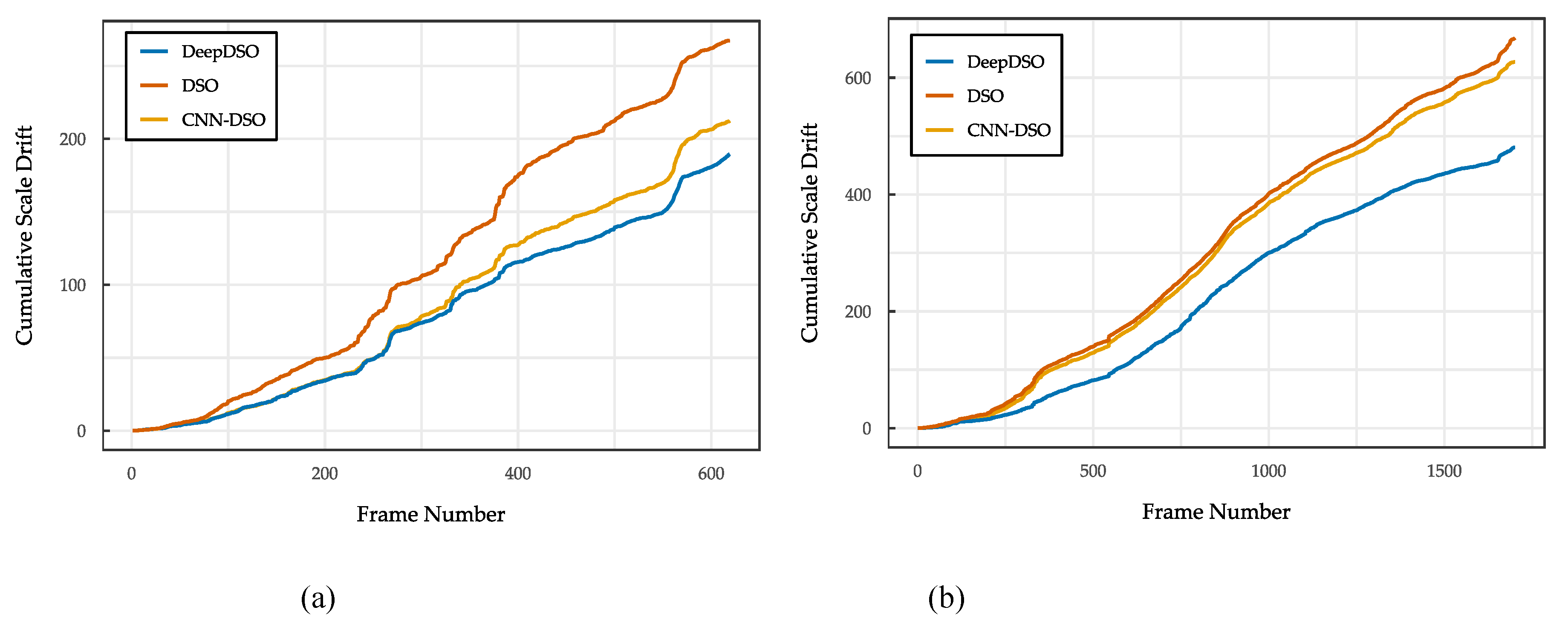

Table 1.
Sensitivity Analysis of Variance Coefficient in Depth Variance Initialization
| Coefficient () | Translational RMSE† | Std. Dev. | Convergence Rate‡ |
| 2 | 0.4127 | 0.0856 | 73% |
| 3 | 0.3214 | 0.0523 | 87% |
| 4 | 0.2685 | 0.0347 | 94% |
| 5 | 0.2453 | 0.0218 | 98% |
| 6 | 0.2382 | 0.0163 | 100% |
| 7 | 0.2491 | 0.0197 | 100% |
| 8 | 0.2738 | 0.0284 | 100% |
| 9 | 0.3156 | 0.0412 | 100% |
| 10 | 0.3647 | 0.0569 | 100% |
†Evaluated on TUM-Mono sequence 29 over 10 forward runs. RMSE values represent alignment error after trajectory alignment. ‡Percentage of runs successfully completing the sequence without tracking failure.
Table 2.
Specifications of the hardware used during experimentation.
| Component | Specifications |
| CPU | AMD Ryzen™ 7 3800X. 8 cores, 16 threads, 3.9 – 4.5 GHz. |
| GPU | NVIDIA GEFORCE RTX 3060. Ampere architecture, 1.78 GHz, 3584 CUDA cores, 12 GB GDDR6X. Memory interface width 192-bit. 2nd generation Ray Tracing Cores and 3rd generation Tensor cores. |
| RAM | 16 GB, DDR 4, 3200 MHz. |
| ROM | SSD NVME M.2 Western Digital 7300 MB/s |
| Power consumption | 750 W1 |
1 Hardware did not reach max power consumption. Avg. load was close to 550 W during experiments.
Table 3.
Medians and Kruskal-Wallis comparisons for each algorithm's translation, rotation, and scale errors.
Table 3.
Medians and Kruskal-Wallis comparisons for each algorithm's translation, rotation, and scale errors.
| Method |
Translation error |
Rotation error |
Scale error |
Start-segment Align. error |
End-segment Align. error |
RMSE |
| Kruskal-Wallis general test | ||||||
| DeepDSO | 0.3250961a | 0.3625576a | 1.062872a | 0.001659008a | 0.002170299a | 0.06243667a |
| DSO | 0.6472075b | 0.6144892b | 1.100516b | 0.003976057b | 0.004218454b | 0.19595997b |
| CNN-DSO | 0.7978954c | 0.9583970c | 1.078830c | 0.008847161c | 0.006651353c | 0.20758145b |
Medians with different letters in the same column differ significantly according to the Kruskal-Wallis test and pairwise Wilcoxon signed rank test for
Disclaimer/Publisher’s Note: The statements, opinions and data contained in all publications are solely those of the individual author(s) and contributor(s) and not of MDPI and/or the editor(s). MDPI and/or the editor(s) disclaim responsibility for any injury to people or property resulting from any ideas, methods, instructions or products referred to in the content. |
© 2025 by the authors. Licensee MDPI, Basel, Switzerland. This article is an open access article distributed under the terms and conditions of the Creative Commons Attribution (CC BY) license (http://creativecommons.org/licenses/by/4.0/).
Copyright: This open access article is published under a Creative Commons CC BY 4.0 license, which permit the free download, distribution, and reuse, provided that the author and preprint are cited in any reuse.


