
Submitted:
06 October 2025
Posted:
08 October 2025
You are already at the latest version
Abstract
High-resolution LiDAR-derived 3D digital outcrop models are essential for detailed geological analysis, but their massive data volumes often exceed the rendering and memory capacities of standard computer systems, posing significant visualization challenges. Although Level of Detail (LOD) techniques are well-established in GIS and computer graphics, they are not directly suitable for the elongated, cliff-face morphology of typical outcrops. This paper presents an automated method for constructing and visualizing LOD models specifically tailored to high-resolution LiDAR outcrops. The workflow begins by segmenting the monolithic model based on texture coverage, followed by building an adaptive LOD tile pyramid for each segment using a pseudo-quadtree approach. A feature-preserving Quadric Error Metric (QEM) simplification algorithm, incorporating boundary freezing and fallback strategies, is employed to retain critical geological structures while significantly reducing geometric complexity. For visualization, a dynamic multi-scale loading and rendering mechanism is implemented using an LOD index with the OpenSceneGraph (OSG) engine. Results demonstrate that the proposed method effectively overcomes the bottleneck of rendering massive outcrop models, enabling smooth, interactive visualization and providing a robust foundation for multi-scale geological interpretation.
Keywords:
digital outcrop model
; level of detail
; LiDAR
; three-dimensional construction
; visualization
1. Introduction
Geological outcrops are important research objects in geological research [1,2,3]. Traditional outcrop studies mainly rely on field investigations, which are limited by terrain and thus cannot effectively survey outcrops located in high or hazardous areas. The emergence of digital outcrop technology has provided new technical means for geological outcrop research [4]. LiDAR (Light Detection and Ranging), as one of the most precise and commonly used digital outcrop acquisition techniques, enables rapid and large-scale collection of high-resolution point cloud data of geological outcrops, with scanning accuracy reaching up to 1mm [5]. Based on these data, high-resolution 3D digital outcrop mesh models with photographic textures can be constructed, allowing for detailed digital representation and analysis of outcrops [6]. Using such high-resolution LiDAR-derived digital outcrop models, geoscientists can conduct lithological and mineral identification [7,8], structural surface interpretation [9], fracture and cavity extraction [10,11], and sedimentary feature description [12] directly at the desktop, thereby greatly improving research efficiency and reducing the cost and intensity of geological exploration.
High-resolution digital outcrop models typically involve massive data volumes. Due to limitations in computer hardware and network bandwidth, it is necessary to employ LOD techniques to reconstruct individual outcrops, generating multi-resolution LOD models that enable efficient rendering in various real-time 3D digital outcrop simulation systems [13]. Although LOD has become a mature technology in fields such as computer vision [14,15], GIS and remote sensing [16,17,18], as well as urban and landscape modeling [19,20,21], its direct application to geological outcrop models presents unique challenges.
First, compared with conventional 3D terrain or urban models, there is no standardized solution for LOD hierarchy division or tile-pyramid construction specifically tailored to outcrop models. Considering the spatial layout, scale, and observation perspectives of outcrop sections, traditional spatial indexing and data partitioning strategies often require adaptive adjustments. Second, digital outcrop models are typically composed of massive, dense, and irregularly distributed 3D point clouds with associated textures. Their surface geometry is highly complex, containing numerous faults, fractures, joints, bedding planes, and other fine geological structures. These microstructures are critically important both visually and geologically, yet they are easily over-smoothed or removed during conventional LOD simplification processes, resulting in the loss of semantic information associated with key geological features. Therefore, it is essential to develop simplification algorithms that prioritize the preservation of detailed geological structures in digital outcrop models. Finally, the extreme data volume and computational demands of large-scale, high-precision digital outcrop models place significant requirements on the scheduling and rendering of LOD models, further highlighting the need for optimized and specialized LOD strategies in the geological domain.
To address these challenges, this paper presents an automated method for constructing and visualizing LOD models specifically designed for high-resolution LiDAR-derived digital outcrops. The proposed workflow first segments the monolithic outcrop model based on texture coverage, followed by the construction of an adaptive LOD tile pyramid for each segment using a pseudo-quadtree approach. A feature-preserving QEM simplification algorithm, incorporating boundary freezing and fallback strategies, is employed to retain critical geological structures while significantly reducing geometric complexity. For visualization, a dynamic multi-scale loading and rendering mechanism is implemented using an LOD index in combination with the OSG engine. The proposed approach effectively mitigates the bottlenecks associated with rendering massive digital outcrop models, enabling smooth, interactive visualization and providing a robust foundation for multi-scale geological interpretation.
2. Related Works
2.1. Digital Outcrops
A digital outcrop refers to a 3D model of a rock exposure that preserves realistic spatial coordinates and texture information, generated through technologies such as remote sensing, photogrammetry, and laser scanning. Since Bryant et al. (2000) systematically elaborated its scientific value, this technology has undergone more than two decades of rapid development and has become an indispensable data foundation in geological modeling, reservoir characterization, and related fields [4].
Among various modeling approaches, LiDAR has consistently maintained a leading position in spatial accuracy, enabling the acquisition of dense point cloud data with millimeter-level precision. In 2005, Bellian et al. first introduced LiDAR systems into geological outcrop investigations and established a complete workflow encompassing data acquisition, processing, and visualization [5]. Building upon this foundation, subsequent studies have enhanced scanning precision, improved point cloud registration algorithms, and developed automated methods for lithological and structural feature extraction [22,23,24]. Over the past two decades, LiDAR-based digital outcrop techniques have matured substantially, achieving accuracies of up to 1 mm. The steadily increasing level of detail and scale of reconstructed models have made LiDAR the most precise and widely adopted approach in digital outcrop research [8,25].
In parallel, photogrammetry-based modeling techniques have developed rapidly. In 2012, Westoby et al. introduced the Structure from Motion (SfM) approach to digital outcrop reconstruction, providing a cost-effective alternative to LiDAR [26]. By matching multiple overlapping images, SfM reconstructs 3D structures efficiently. With the widespread availability of unmanned aerial vehicles (UAVs), it has become possible to capture centimeter-scale detail and achieve full-coverage reconstructions of complex outcrops. Comparative analyses conducted in 2016 confirmed the high consistency between SfM-derived models and terrestrial laser scanning results [27]. Since then, the integration of UAV-based oblique photogrammetry has further enriched digital outcrop workflows, leading to a mature technical framework and a growing number of successful applications [28,29,30,31].
More recently, digital outcrop modeling has entered a phase of multi-source data integration. The high geometric accuracy of LiDAR and the rich texture information captured by photogrammetry offer complementary advantages. Furthermore, the incorporation of additional data sources such as GPS measurements and remote sensing imagery has transformed digital outcrops from isolated 3D models into comprehensive geospatial information platforms [32,33]. This fusion enables multiscale geological feature recognition and extends the application of digital outcrops to structural interpretation, reservoir modeling, fracture characterization, and lithological or mineral identification [6,7,8,9,10,11,12,34,35].
However, as data volumes continue to grow, efficient data organization and hierarchical indexing have become critical challenges. Achieving a balance between geological accuracy and interactive visualization performance is essential for supporting large-scale analysis and interpretation. In this context, LOD construction and visualization technologies play a vital role in overcoming current computational bottlenecks and enabling efficient, scalable digital outcrop representations.
2.2. Level of Detail
The concept of Level of Detail (LOD) was first introduced by Clark (1976), who proposed reducing real-time rendering and transformation overheads through multiresolution geometric representations [36]. Early research primarily focused on geometric simplification algorithms within computer graphics, such as edge-collapse based progressive meshes [37] and hierarchical structures built upon quadtrees or octrees [38]. These methods facilitated multi-level representations and dynamic switching between resolutions based on viewing distance. With the advancement of graphics hardware and real-time rendering capabilities, the LOD concept has gradually extended beyond geometry to encompass textures and shading. Techniques such as mipmap-based multiresolution texture mapping and GPU-driven dynamic detail scheduling have significantly enhanced rendering efficiency for large-scale and complex scenes [39].
In the field of 3D city modeling, the notion of LOD has been redefined to describe the level of geometric and semantic detail representing real-world spatial entities at different scales. The CityGML standard, for instance, classifies city objects into five discrete levels (LOD0–LOD4), enabling multiscale spatial analysis, visualization, and data exchange [40]. Nevertheless, such discrete classifications are limited in their ability to express continuous scale variations and maintain semantic consistency. To address these limitations, later studies proposed continuous or quasi-continuous LOD models [41] and explored variable-resolution modeling approaches based on multiscale spatial hierarchies and hierarchical indexing [42], thereby supporting seamless transitions and multilevel management from local to regional scales.
In recent years, driven by the rapid progress of GIS, remote sensing, photogrammetry, and LiDAR technologies, LOD research has expanded to encompass high-density geospatial datasets such as point clouds, digital city models (DCMs), digital terrain models (DTMs), and digital surface models (DSMs) [16,17,18]. These developments have sought to overcome performance bottlenecks in online visualization and sharing of large-scale geospatial models through multiscale data organization and streaming-based rendering strategies.
Within the context of digital outcrop models, LOD technology plays an equally crucial role, particularly for managing large-scale geological point clouds and high-resolution surface reconstructions. By introducing hierarchical levels of detail, digital outcrop model visualization can maintain spatial accuracy while reducing computational load, thus enabling efficient multiscale exploration and analysis. However, most existing LOD techniques have originated from general-purpose graphics or urban modeling domains and are not tailored to the specific structural and semantic characteristics of geological data. As a result, challenges remain in maintaining geological feature fidelity, allocating texture resolution adaptively, and preserving semantic consistency across scales.
However, prior research on digital outcrops has largely concentrated on data acquisition and geological interpretation [43,44,45,46], with relatively limited attention to LOD organization or hierarchical design strategies suited to geological data characteristics [47,48]. Future work should therefore aim to establish task-oriented, adaptive LOD modeling frameworks driven by geological research objectives. Such approaches will enable intelligent detail selection, improve scalability, and strengthen the role of LOD technologies in digital outcrop model construction, sharing, and visualization—ultimately advancing geoscientific research toward intelligent, multiscale cognition.
3. Methods
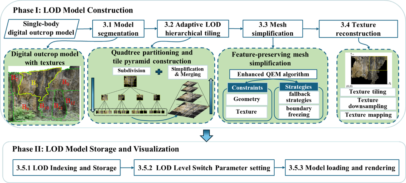
To achieve the construction and visualization of LOD models for high-resolution LiDAR-based digital outcrops, we propose an automated solution that integrates model simplification, LOD index construction, and multi-scale rendering. As illustrated in Figure 1, the entire workflow comprises seven sequential steps, organized into two primary phases:
Phase I: LOD Model Construction
- 1.
- Single-body model Segmentation (Section 3.1): Import the high-resolution, large-scale LiDAR-derived single-body digital outcrop model, then partition it into multiple sub-models according to the coverage area of each texture image.
- 2.
- Adaptive LOD Hierarchical Tiling (Section 3.2): For each sub-model, construct a multi-level LOD tile structure using a pseudo-quadtree partitioning approach, forming a tile pyramid through iterative subdivision, simplification, and merging processes.
- 3.
- Mesh Simplification (Section 3.3): Apply a feature-preserving QEM algorithm to simplify each tile across all LOD levels, incorporating constraints for geometry and texture preservation along with strategies such as fallback tactics and boundary freezing.
- 4.
- Texture Reconstruction (Section 3.4): Reconstruct texture images and their corresponding coordinates for tiles at each LOD level, involving texture tiling, downsampling, and remapping operations.
Phase II: LOD Model Storage and Visualization
- 5.
- LOD Indexing and Storage (Section 3.5.1): Establish an LOD index file for the entire model, storing geometric data, texture information, and other parameters of each constructed tile in OSGB format.
- 6.
- Display Parameter Setting (Section 3.5.2): Configure model display parameters based on the texture image size of each tile to optimize visualization quality.
- 7.
- Model Loading and Rendering (Section 3.5.3): Implement multi-scale loading and rendering of the LOD digital outcrop model using the OSG engine, enabling efficient visualization across different detail levels.
In summary, this solution realizes the construction and visualization of LOD for high-resolution LiDAR-derived digital outcrop models through seven steps in two phases, and the following will elaborate on the specific implementation methods and technical details of each step.
3.1. Single-body Model Segmentation
The original model used for LOD construction is a LiDAR-derived single-body digital outcrop model. LiDAR technology acquires high-density point cloud data from outcrop surfaces, which are triangulated to generate a high-resolution mesh. High-resolution photographic images are then applied through texture mapping to produce a photorealistic 3D model (Figure 2(a)). A single-body digital outcrop model generally consists of two core components: (1) geometric data: three-dimensional meshes generated by triangulating laser-scanned point clouds to accurately represent outcrop morphology (Figure 2(c)); and (2) texture data: high-resolution images captured by digital cameras and mapped onto the mesh surface to provide realistic visualization (Figure 2(b)).
To preserve the integrity of the original texture mapping, the digital outcrop model is first subdivided into multiple sub-models B = {B0, B1, B2, …} based on the coverage of texture images on the model surface (Figure 2(a)). Subsequently, a quadtree-based tile pyramid is built for each sub-model, resulting in a multi-scale LOD tiled structure described in the following sections. This method ensures geometric accuracy and texture fidelity while reducing the complexity of texture reconstruction during LOD construction.
3.2. Adaptive LOD Hierarchical Tiling
To achieve efficient multiscale organization of complex outcrop models, this section proposes an adaptive LOD tiling strategy that integrates a bottom-up simplification process with quadtree-based hierarchical partitioning. The process first applies quadtree subdivision in texture space to generate fine-grained bottom-level tiles, and then progressively simplifies and merges them to construct upper-level LOD nodes.
3.2.1. Bottom-Level Tile Generation Based on Quadtree Partitioning
The quadtree index was first proposed by Tayeb in 1998 [49]. Its basic principle is to recursively divide a rectangular region into four subregions until the number of elements in each subregion does not exceed a specified capacity. In this study, the sub-models are partitioned in the 2D texture coordinate space using a quadtree structure, resulting in a multi-level, hierarchically refined tile pyramid. A key question is how many levels of subdivision are appropriate for each sub-model. Here, we adopt the data volume of a single tile node as the criterion for further subdivision. Since each subdivision divides one tile into four child tiles, under the assumption of uniform data distribution, the data volume of each child tile is approximately one quarter of its parent. We define a threshold Vt (e.g., 1.0 MB) such that the data volume of each node in the constructed LOD structure is close to this threshold, enabling efficient loading and network transmission during rendering. Subdivision is terminated once the data volume of a single tile falls below Vt. Accordingly, the number of quadtree subdivision levels can be estimated as:
where V0 denotes the data volume of the original sub-model, Vt is the predefined data volume threshold for a single tile, and n is the estimated number of subdivision levels in the quadtree.
Based on the above idea, performing n quadtree subdivisions on a given sub-model yields the bottom-level tile data, whose resolution remains consistent with the original model without any simplification (see Figure 3). Obviously, the valid part of a texture image is not necessarily a regular rectangle, and the black regions represent invalid areas. If a tile’s coverage falls entirely within an invalid area, that tile will be treated as an invalid node and ignored in subsequent processing.
3.2.2. Simplification and Merging Strategies for Bottom-Up Tile Generation
After the above quadtree subdivisions, we have obtained the bottom-level tiles of the LOD model. Next, the remaining tiles at higher levels of the LOD model are generated gradually using a bottom-up strategy that simplifies and merges tiles simultaneously. Suppose the simplification ratio between two adjacent levels from bottom to top in the LOD model is θ. According to the previously proposed simplification algorithm, each tile’s mesh is simplified individually, while its texture image is also correspondingly downsampled. Figure 4 demonstrating how the simplification and merging operations are flexibly applied according to data size thresholds when generating higher-level tiles in a bottom-up LOD construction. Consider four tiles at level i that belong to the same parent node in the previous quadtree subdivision (Nodei,0, Nodei,1, Nodei,2, Nodei,3). First, the total data size for the simplified level i-1 is estimated as:
where , , , and are the data size of the four tiles at level i, θ is the simplification ratio.
If Vi-1 < Vt, four corresponding simplified tiles at the upper level are merged into a single parent node (see Figure 4(a)); othewise, they remain unmerged and are preserved as four separate upper-level nodes, each corresponding to a lower-level node (see Figure 4(c)). During this process, the correspondence between nodes in adjacent levels is also established, forming either one-to-one or one-to-four relationships (see Figure 4(b) and (d)).
3.3. Feature-preserving Mesh Simplification
In the construction of the tile pyramid, model simplification is a critical step, as each tile consists of both geometric (mesh) and texture components. During the hierarchical simplification process, it is essential to preserve these geometric and texture features as much as possible. For textured mesh simplification, Garland et al. introduced an edge-collapse algorithm based on QEM [37], which is computationally efficient and produces simplified models of good quality [50]. However, when applied to the construction of LOD models for digital outcrops, additional optimization and customization are necessary. To this end, we propose a feature-preserving QEM simplification algorithm, which incorporates tailored constraints to simultaneously preserve geometric and texture features of digital outcrop models. Specifically, for texture preservation, we extend the QEM framework by integrating texture coordinates; for geometric preservation, we introduce a vertex sharpness constraint to retain fine surface details; and under specific conditions, we further design dedicated edge-collapse strategies to better maintain detailed features in the simplified model.
3.3.1. Simplification and Merging Strategies for Bottom-Up Tile Generation
The QEM algorithm is an edge collapse simplification algorithm. In mesh simplification via the edge collapse method, an edge (V1, V2) is considered the basic operation unit, and its vertices V1 and V2 are contracted to a single point v0 (see Figure 1). It calculates the sum of squared distances from the new vertex V0 in space to each triangular face in the one-ring neighborhood of the original edge (V1,V2) as the error metric for edge collapse, thereby optimizing the selection of edges to collapse. However, for the simplification of textured mesh models, the optimization of texture coordinates at the new vertex after collapse must also be considered. To address this, Garland et al. extended the foundational QEM algorithm by incorporating attribute features such as texture coordinates (u, v) alongside the three-dimensional coordinates (x, y, z) of the vertices [50]. This constructs a multidimensional space for the model and calculates the quadratic error of vertices within this multidimensional space. Through the minimization of the quadratic error matrix, the optimal spatial coordinates and texture coordinates for each vertex in the abstract multidimensional space are determined. In the described multidimensional space, a quadratic error matrix Qi can be calculated for each triangular face within the one-ring neighborhood of any vertex Vi. Consequently, the error of collapsing an edge (V1,V2) is expressed as:
where V0=[ x0,y0,z0,u0,v0,1]T is the high-dimensional homogeneous coordinate of the new vertex. Q1 and Q2 are the error matrices of V1 and V2, respectively. E(V0) is determined by the position of the new vertex.
E(V0)=V0T(Q1+Q2)V0
3.3.2. Vertex Sharpness Constraint
Compared to the smooth parts of the model, the concave and convex parts represent significant geometric structural features and should be preserved as much as possible during simplification. To enhance the algorithm’s sensitivity to these concave and convex regions, ensuring that more detailed features are retained even under high simplification ratios, we introduce vertex sharpness α as a constraint factor for modeling geometric detail characteristics. As illustrated in Figure 5, the calculation involves, for any vertex in the model, iterating through its one-ring neighborhood to compute the angles (in radians) between the normal vectors of every pair of adjacent triangular faces. The sum of these angles is then weighted and averaged using the corresponding triangle areas to measure the vertex’s sharpness. We define α as the vertex sharpness of a point in the mesh, and the corresponding calculation formula is shown in Equation (4).
where α is the vertex sharpness, n is the number of triangles in the one-ring neighborhood of the vertex, Ssum is the total area of these triangles, Si represents the area of the i-th triangle, and Ni represents the normal vector of this triangle.
Integrating the fundamental QEM error function from Section 3.2.1 with the vertex sharpness constraint factor, we propose a new error function as shown in Equation (5):
where α1 and α2 are the vertex sharpness of V1 and V2, respectively. The meanings of other parameters are the same as those in Equation (3). Our goal is to find the V0 that minimizes the E(V0). This is a classic quadratic optimization problem. The error function E(V0) is a quadratic function with respect to V0. To find its minimum, we take its gradient and set it to zero:
E(V0)=V0T( α1Q1+α2Q2)V0
∇E(V0)= 2(α1Q1 +α2Q2) V0= 0
Letting Q = α1Q1 +α2Q2 , the problem reduces to solving the linear system:
QV0 = 0
However, the matrix Q may be singular (non-invertible), for example, when all associated planes are coplanar or collinear. In such cases, the algorithm needs to adopt a fallback strategy.
3.3.3. Strategies for Specific Cases
Since our simplification algorithm is specifically designed for constructing LOD models—where the model is divided into tiles during LOD structure creation—we introduce a tile boundary freezing strategy (Strategy 1) to maintain topological and texture continuity between adjacent tiles. Meanwhile, when the Q matrix in the error function is singular, the equation QV0 = 0 has no solution or no unique solution. In such cases, three fallback strategies (Strategies 2–4) can be employed. In summary, the following four strategies are applied depending on the situation :
The decision tree for selecting these strategies is illustrated in Figure 7. The process first checks if the candidate edge is located on a tile boundary—if true, it immediately applies Strategy 1 by assigning infinite collapse cost to prohibit collapse. For non-boundary edges, it then checks if matrix Q is singular; if not, it directly computes the optimal solution using V0= = -Q⁻¹b. If Q is singular, a fallback strategy is triggered based on the edge properties. For texture seams, the point minimizing the error function along the edge is selected to preserve texture integrity (Strategy 2); for non-seam edges, the risk of generating degenerate or flipped faces is assessed—if high, the vertex with the smaller QEM error (V1 or V2) is chosen (Strategy 3), otherwise the edge midpoint is selected for stability (Strategy 4). Finally, the collapse error of the edge is calculated to update the simplification priority queue.
3.4. Tile Texture Downsampling and Remapping
During the construction of the tile pyramid, adaptive hierarchical partitioning is achieved through bottom-up tiles simplification and merging. In this process, texture images are simultaneously divided into smaller rectangular tiles, thereby disrupting the original texture mapping relationships. Consequently, for each tile unit, in addition to mesh simplification (see Section 3.3), texture downsampling and remapping must be performed in a bottom-up manner.
To ensure that texture downsampling ratio corresponds to the degree of geometric simplification, the downsampling window size is set as the reciprocal of the simplification ratio (e.g., when the simplification ratio θ = 0.5, the downsampling window size is 2). As image downsampling is a mature technique, it is not further elaborated here. Texture coordinate remapping aims to establish a correspondence between the original global texture coordinate space and the local coordinate space of each tile (see Figure 8). For any tile at a given LOD level, the new texture coordinates of its vertices are computed as follows:
where u and v represent the original texture coordinates of a vertex in the global texture space; umin, vmin, umax, and vmax define the bounding range of the textrue region covered by the tile in the original global texture space; and u’ and v’ represent the transformed texture coordinates after remapping. They correspond to the local coordinate system of the tile’s cropped texture image, ensuring that the texture aligns correctly with the simplified mesh.
3.5. LOD Model Storage and Visualization
To ensure efficient management, storage, and visualization of large-scale outcrop models, a multi-level LOD structure must be systematically organized, stored, and rendered. This section introduces the design of the LOD indexing and storage structure, and the OSG-based visualization mechanism, including parameter settings and dynamic loading strategies.
3.5.1. LOD Indexing and Storage
After model partitioning and tile pyramid construction, the single-body model is decomposed into multi-level discrete sub-blocks (sub-models or tiles), which must be organized through an appropriate spatial index to enable the 3D visualization module to dynamically schedule and render them according to the viewport state.
As described in Section 3.1, the single-body model is divided into multiple sub-models, and then a tile pyramid is constructed for each sub-model (see Figure 9(a)). Given that the digital outcrop exhibits a banded façade, a regular grid is used to construct the top-level spatial index of the sub-models. The outcrop profile is partitioned along its major axis into several equally sized rectangular grids, and each sub-model Bi is assigned to the grids it overlaps or intersects, thereby forming the top-level grid index of the entire outcrop model. In practice, we traverse all sub-model data blocks, compute the centroid of each sub-model, and then assign the sub-model to the grid cell that contains its centroid.
As show in Figure 9(b), in this indexing structure, the node representing the entire model extent serves as the root node (Level 0). Each rectangular grid corresponds to a level-1 node, and the nodes associated with the sub-models linked to these grids are defined as level-2 nodes. From Level 2 downward, the nodes correspond to the tile pyramid generated by further subdivision of each sub-model. The logical structure of this pyramid has been described in detail in Section 3.2. To index these tiles, we construct a spatial index that approximates a quadtree, following the pyramid hierarchy from top to bottom. During the bottom-up tile generation process, parent–child relationships can be either one-to-four or one-to-one, resulting in a quadtree-like hierarchy. We therefore refer to this structure as a pseudo-quadtree. Unlike a standard quadtree, where each parent node has exactly four children, the pseudo-quadtree allows more flexible relationships between levels.
Following the multi-level indexing structure, the constructed LOD model is stored in the OSGB format. OSGB is a binary storage format that supports LOD structures. Typically, a single OSGB 3D model dataset contains multiple folders, and each folder includes several OSGB files. Each OSGB file contains one root node (Root), several intermediate-level nodes (of type Group or Geode), and the leaf nodes (of type Geode). The intermediate nodes store information such as geometry, textures, and parent–child relationships between hierarchical levels, while the leaf nodes only contain the geometric and texture information of the model. This design is fully compatible with the constructed LOD indexing structure and facilitates efficient visualization of LOD 3D models based on the OSG engine.
3.5.2. LOD Level Switch Parameter
In OSG, node switching follows the “near-large, far-small” principle of LOD visualization, controlled by the RangeList parameter. To improve adaptability, this study adopts the screen-pixel–based RangeMode, which determines LOD switching according to the model’s projected pixel size, avoiding the limitations of distance-based thresholds. Figure 10 illustrates the geometric basis for screen-pixel–based LOD switching used in this work: (a) the camera frustum, viewport and the model’s bounding sphere in 3D; (b) a 2D cross-section that shows the viewing angle, the distance d from the camera to the bounding-sphere center, and the viewport plane. Let D denote a representative model size (we use the bounding-sphere diameter) and let γ and H be the vertical field of view and the viewport height in pixels, respectively (see Figure 10(b)). The model’s projected height in pixels P can be expressed as
so that
In implementation we compare P with the tile texture size St (in pixels) and set the RangeList threshold so that when P reaches the maximum allowable screen size (Pixelsize_max), the engine loads a higher-resolution sub-node. Practically, we take Pixelsize_max = St. Note that using the bounding sphere gives a conservative, inexpensive estimate; for irregular sub-models one may alternatively use the projected diagonal of the bounding box or the nearest-point distance to avoid popping at close range.
3.5.3. LOD Model Loading and Rendering
This study utilizes the PagedLOD and DatabasePager classes in OSG to organize and schedule LOD models, supporting large-scale digital outcrop visualization in both desktop and web environments. The core idea is to display visible elements within the current view while preloading potentially visible elements and unloading those unlikely to be seen soon. This ensures limited in-memory data, preventing rendering lag or data loss during scene browsing.
As shown in Figure 11, PagedLOD dynamically loads model nodes (tiles or sub-models) of different detail levels based on the viewing range, enabling paged LOD rendering. Unlike static loading, the database loads or removes nodes dynamically as the viewpoint changes, significantly reducing memory and computation costs. The DatabasePager class manages node scheduling by unloading scene subtrees outside the current view and loading new ones entering the view. It maintains nodes through queues and supports separate threads for local and remote data. For network data, a cache path (OSG_FILE_CACHE) can be set to store downloaded models locally, further improving rendering efficiency and responsiveness.
4. Results
To verify the feasibility and effectiveness of the proposed LOD construction and visualization method, experiments and tests are conducted on the LOD construction tasks of two high-resolution point cloud outcrop models.
4.1. Experimental Dataset and Environment
Two outcrop profiles located in the Sichuan Basin, China, were selected as data sources for the experiments. They are the Gaojiashan outcrop profile of the Dengying Formation (Sinian System) and the Panlongdong outcrop profile of the Changxing Formation (Permian System):
Model 1: The Gaojiashan Dengying Formation outcrop is located approximately 0.5 km north of Gaojiashan Village, Hujia Town, Ningqiang County, Sanxi Province. It is distributed in a strip-like shape along the roadside, with a total length of about 0.85 km.
Model 2: The Panlongdong Changxing Formation outcrop is located beside the highway near Panlongdong in Jichang Town, northeastern Xuanhan County, Sichuan Province. It extends in a northeast–southwest direction along the river, with a profile length of about 0.75 km.
During data acquisition, a RIEGL VZ-400 terrestrial laser scanner was used to capture high-resolution 3D point clouds of the outcrop surfaces, and a Pentax 645D high-resolution digital camera was used to obtain high-quality texture images. Subsequently, high-fidelity 3D digital outcrop models with realistic textures were generated through processes such as point cloud registration and thinning, triangular mesh construction, and texture mapping. The single-body models were stored in OBJ format. Figure 12 shows the visualization results of the two large-scale digital outcrop models used in the case study. The basic information of the two constructed single-body models is listed in Table 1.
The constructed single-body digital outcrop models contain massive amounts of data, which can easily lead to issues such as insufficient memory, lagging performance, and visual artifacts like jumping or missing scenes during model loading and scene switching. Therefore, it is necessary to perform LOD reconstruction on the single-body models. The proposed LOD-based digital outcrop modeling method was implemented under the development environment of Windows 10, Visual Studio 2017, and OSG 3.6. A 3D visualization tool for digital outcrops was developed using visualization techniques to enable multi-scale loading and real-time browsing of LOD models, significantly improving computational efficiency. The hardware configuration of the computer used for the experiments is as follows: Intel Core i7-11700K @ 3.60 GHz processor, 16.0 GB RAM, and NVIDIA GeForce GTX 1650 graphics card. All algorithms and tools mentioned above were implemented based on the OSG 3D visualization open-source library and the C++ programming language. The detailed visualization results will be presented in the following sections.
4.2. Results and Analysis of LOD Models Construction and Visualization
LOD structures were constructed for the two single-body models obtained during the data acquisition stage. In this experiment, the model simplification ratio θ was set to 0.8, and the tile data size threshold Vt was set to 1.0 MB. During the process, the computer’s performance was monitored, and the algorithm’s execution time (s), average memory usage (MB), and average CPU usage (%) were recorded. For Model 1, the generation time of the LOD model was 8424 seconds, with an average CPU utilization of approximately 9.6% and an average memory usage of about 2651.7 MB. For Model 2, the LOD model generation took 13,428 seconds, with an average CPU utilization of approximately 11.6% and an average memory usage of about 3352.7 MB. The basic information of the two constructed LOD models are summarized in Table 2.
The purpose of constructing LOD models is to minimize the loading time and memory consumption of large-scale, high-resolution 3D digital outcrop models, thereby reducing the hardware requirements during visualization and improving rendering efficiency. To evaluate the effectiveness of this approach, the generated LOD models were imported into an OSG-based 3D visualization window. Key performance indicators were collected for the LOD models, including model loading time, memory usage after loading, display frame rate, and the number of stuttering occurrences during roaming. These indicators were then compared with those of the original single-body models. Based on this comparison, a comprehensive assessment of the LOD models’ visualization performance was conducted.
As shown in Table 3, for Model 1, the LOD model had an average CPU usage of 15%, memory usage after loading of 188 MB, a loading time of 3.7 seconds, and a display frame rate of 59.7 FPS. In comparison, the original model had an average CPU usage of 20%, memory usage after loading of 3506 MB, a loading time of 117.5 seconds, and a display frame rate of 6.7 FPS. Compared with directly loading the full model, the LOD model reduced average CPU usage by 25%, memory usage by 94.6%, loading time by 96.7%, and increased frame rate by 656.7%. For Model 2, the LOD model had an average CPU usage of 13.4%, memory usage after loading of 112 MB, a loading time of 4.1 seconds, and a display frame rate of 59.8 FPS. The original model had an average CPU usage of 20.2%, memory usage after loading of 11,602 MB, a loading time of 550.7 seconds, and a display frame rate of 1.2 FPS. Compared with directly loading the full model, the LOD model reduced average CPU usage by 33.7%, memory usage by 99.0%, and loading time by 99.2%.
In addition, we measured and recorded the frame rate of the model at various camera distances. Here, the viewing distance refers to the distance between the camera and the model. The LOD model loading and scheduling mechanism dynamically adjusts the model’s level of detail according to the viewing distance. We divided the distance from the viewpoint to the model within the view frustum into 10 equal intervals, representing 10 discrete levels. Lower levels correspond to shorter distances, where the model is closer to the viewpoint and displays higher detail; conversely, higher levels correspond to greater distances, where the model is farther from the viewpoint and displays lower detail. Figure 13 presents the frame rate statistics of the model with and without LOD across these different viewing distances.
As shown in the Figure 13, Model 1 with LOD exhibits higher frame rates, remaining at the screen refresh rate limit once the viewing distance decreases to 8. In contrast, the frame rates of the non-LOD model increase gradually as the viewing distance decreases, with stable values of 6.7 FPS, 9.8 FPS, 18.7 FPS, 31.7 FPS, and 39.1 FPS, respectively. Similarly, Model 2 with LOD maintains a high frame rate, around 60 FPS, whereas the frame rates of the non-LOD model rise gradually with decreasing viewing distance, with stable values of 1.2 FPS, 1.6 FPS, 2.4 FPS, 6.7 FPS, and 14.1 FPS, respectively. These results indicate that models with LOD achieve significantly higher frame rates across different viewing distances.
Furthermore, we present the actual rendering results of local regions of the LOD models at different viewing distances (see Figure 14 and Figure 15, from (a) to (e), with the viewpoint progressively approaching the model). It can be observed that across all viewing distances, the geometric structure of the model remains stable, tile seams are tightly aligned without gaps, and the visual transitions during multi-detail tile scheduling are smooth, resulting in consistently high visual quality.
4.3. Comparative Analysis of Simplification Algorithm Results
While Section 4.2 demonstrated the visual results and scalability of our constructed LOD models, this section quantitatively validates the effectiveness of our proposed simplification algorithm. As the core component responsible for feature preservation and smooth visual transitions, the simplification algorithm’s performance is critical. We conducted a comparative experiment pitting our algorithm against two established methods: the foundational QEM [16] and the MeshLab QEM-based simplification [51].
The experiment tested ten different simplification rates for each algorithm on Model 2 , evaluating their ability to preserve both geometric and textural features. The simplification error was measured using the following two criteria:
Geometric Error: The two-way Hausdorff distance was used to quantify the maximum geometric deviation between the original model M1 and the simplified model M2. It is defined as [17]:
where h(M1, M2) is the one-sided (or directed) Hausdorff distance from M1 to M2, and is the one-sided Hausdorff distance from M2 to M1.
Texture Error: Texture fidelity was quantified following the methodology of [52]. For each model, we captured six directional images (front, back, left, right, up, down) before and after simplification. The Root Mean Square (RMS) of the pixel brightness difference was computed as:
where Y and Y’ denote images before and after simplification, m×n is image resolution, and c = 6 is the number of directions.
The results of geometric and texture errors in model simplification are shown in Figure 16. In terms of geometric error testing, the geometric errors of all three simplification methods gradually increase with higher simplification rates. When the simplification rate exceeds 45-55%, the geometric error of our algorithm becomes slightly larger than the other two methods. This increased geometric error may be attributed to our algorithm’s consideration of more local detail features and texture characteristics, leading to a slight increase in global integration error. Regarding texture error testing, the texture errors of all three methods also increase with higher simplification rates, but our algorithm achieves the smallest texture error, while the QEM algorithm exhibits the largest. This demonstrates the effectiveness of the constraints and strategies designed in our algorithm for texture protection.
We compared the visual effects of different simplification results, taking the simplified model with a 70% simplification rate derived from experiments as an example. At higher simplification rates, the resulting models are more prone to issues such as texture deviation, stretching, and cracks. The visual effect evaluation aims to examine whether the model can maintain the stability of overall appearance attributes and detailed texture features at the highest possible coarsening rate. The visual results for Model 2 are shown in Figure 17. It is evident that the models simplified using the QEM and MeshLab algorithms show significant texture distortion on the outcrop surface, including loss of local details and fragmentation along texture seams. In contrast, our method better preserves both the geometric details and complex texture characteristics of the original model, effectively meeting the application requirements for LOD reconstruction in digital outcrop modeling.
5. Discussion
5.1. Potential Limitations of the Tiling Method
The adaptive LOD hierarchical tiling method proposed in this study is primarily designed for spatial partitioning of elongated, facade-like outcrop profiles. While it adapts well to most scenarios, it may not perfectly accommodate outcrops with highly complex geometries or significant surface undulations. For instance, a profile containing extremely intricate folds could lead to suboptimal model segmentation, resulting in poor visualization outcomes. Therefore, future work should explore classification-based solutions tailored to different morphological types of outcrop profiles. For example, a highly adaptive hybrid method combining quadtree and octree structures could be designed based on geometric features of the outcrop surface, such as curvature, normal variation, and relief intensity [17].
5.2. Empirical and Generalizability Concerns in Algorithm Parameters
The model simplification ratio and tile data volume threshold in the current method may rely on practical application requirements and manual experience. In our experiments, the simplification ratio was set to 0.8, and the tile data threshold was set to 1.0 MB. While these settings are relatively straightforward to implement, they may not optimally suit all scenarios. Considering common network bandwidth limitations, controlling individual tile data within 1.0MB helps reduce loading latency and improves data scheduling efficiency. However, when the model does not need to be loaded and displayed in a network environment, this threshold can be increased, for example, setting it to 3.0 MB would accommodate most desktop application environments. In our implementation, the simplification ratio simultaneously controls both mesh simplification and texture downsampling. In practice, however, there may be more specific requirements for the degree of simplification in each. Thus, the next step involves developing adaptive methods that independently recommend suitable parameters for both aspects, automatically deriving near-optimal values based on input model statistics, such as point cloud density, geometric complexity, and texture resolution.
5.3. Directions for Algorithm Performance Improvement
The current algorithm primarily focuses on the usability of LOD model construction and visualization, with insufficient consideration for computational efficiency. In our experiments, LOD construction and visualization were performed separately. The construction process is relatively time-consuming, which somewhat restricts iterative model updates and real-time preview capabilities. The core issue lies in the highly serialized execution mode of the algorithm. Numerous parallelizable computational tasks, such as triangle traversal, error metric calculation, and vertex clustering decisions, are currently executed sequentially, forming a performance bottleneck. To address this, the key direction for future improvement is to restructure the algorithm for parallelism, leveraging the massive parallel computing capability of GPUs to achieve orders-of-magnitude performance gains [53].
6. Conclusions
This paper has presented a comprehensive LOD-based solution for the efficient visualization of large-scale, high-resolution LiDAR digital outcrop models. The key contributions of this work are threefold:
First, we designed a tailored LOD construction pipeline that integrates model segmentation, pseudo-quadtree tiling, feature-preserving simplification, and texture reconstruction. This workflow effectively addresses the unique challenges posed by the elongated and vertical nature of digital outcrops, overcoming the limitations of conventional LOD methods designed for planar or large-area models.
Second, we developed and integrated key algorithmic optimizations. The incorporation of boundary freezing and fallback strategies into the feature-preserving QEM algorithm ensured the protection of both geometric integrity at tile borders and critical geological features during aggressive mesh simplification.
Finally, we established an efficient data organization and dynamic visualization framework. By employing an LOD index and OSG PagedLOD mechanism, we achieved real-time, view-dependent loading and seamless multi-scale rendering of high-resolution LiDAR-derived digital outcrop models on standard computer hardware.
In summary, this method provides a practical and effective solution for managing and visualizing massive digital outcrop models, directly addressing the critical bottleneck of rendering performance. The generated, well-structured LOD data not only facilitates current geological analysis but also paves the way for future enhancements, such as the seamless integration of semantic attributes and the development of web-based collaborative interpretation platforms. Future work aims to enhance the algorithm’s generalizability, the adaptability of its parameters, and its computational efficiency.
Author Contributions
Conceptualization, Jingcheng Ao and Yuangang Liu; Formal analysis, Ran Jing and Shaohua Li; Methodology, Jingcheng Ao, Yuangang Liu, Bo Liang and Ran Jing; Software, Jingcheng Ao, Yuangang Liu and Bo Liang; Validation, Yanlin Shao and Shaohua Li; Writing – original draft, Jingcheng Ao, Bo Liang , Yanlin Shao, Ran Jing and Shaohua Li; Writing – review & editing, Yuangang Liu. All authors will be updated at each stage of manuscript processing, including submission, revision, and revision reminder, via emails from our system or the assigned Assistant Editor.
Funding
This work was supported by the National Natural Science Foundation of China (Grants No. 42172172).
Data Availability Statement
The data presented in this study are available on request from the corresponding author.
Acknowledgments
The authors would like to express their gratitude to the PetroChina Research Institute of Petroleum Exploration & Development for providing the resources required to collect the dataset used in this study. Additionally, special thanks go to the editor and anonymous reviewers for their constructive comments that substantially improve the quality of the paper.
Conflicts of Interest
This study was supported by the National Natural Science Foundation of China (Grant No. 42172172). Author Bo Liang is employed by PetroChina Liaohe Oilfield Company. The funder and the company had no role in the study design, data analysis, decision to publish, or preparation of the manuscript. The remaining authors declare that they have no competing interests.
References
- Aydin, A. (2000). Fractures, faults, and hydrocarbon entrapment, migration and flow. Marine and petroleum geology, 17(7), 797-814.
- Rimmer, S. M. (2004). Geochemical paleoredox indicators in Devonian–Mississippian black shales, central Appalachian Basin (USA). Chemical Geology, 206(3-4), 373-391.
- Howell, J., Martinius, A. and Good, T. 2014. The application of outcrop analogues in geological modelling: a review, present status and future outlook. Geological Society, London, Special Publications 387, 1-25.
- Bryant, I., Carr, D., Cirilli, P., Drinkwater, N., McCormick, D., Tilke, P., & Thurmond, J. (2000). Use of 3D digital analogues as templates in reservoir modelling. Petroleum Geoscience, 6(3), 195-201.
- Bellian, J. A., Kerans, C., & Jennette, D. C. (2005). Digital outcrop models: applications of terrestrial scanning lidar technology in stratigraphic modeling. Journal of sedimentary research, 75(2), 166-176.
- Liang, B., Liu, Y., Shao, Y., Wang, Q., Zhang, N., & Li, S. (2022). 3D quantitative characterization of fractures and cavities in Digital Outcrop texture model based on Lidar. Energies, 15(5), 1627.
- Jing, R., Shao, Y., Zeng, Q., Liu, Y., Wei, W., Gan, B., & Duan, X. (2025). Multimodal feature integration network for lithology identification from point cloud data. Computers & Geosciences, 194, 105775.
- Shao, Y., Li, P., Jing, R., Shao, Y., Liu, L., Zhao, K., ... & Li, L. (2025). A Machine Learning-Based Method for Lithology Identification of Outcrops Using TLS-Derived Spectral and Geometric Features. Remote Sensing, 17(14), 2434.
- Riquelme, A. J., Abellán, A., Tomás, R., & Jaboyedoff, M. (2014). A new approach for semi-automatic rock mass joints recognition from 3D point clouds. Computers & geosciences, 68, 38-52.
- Wu, S., Wang, Q., Zeng, Q., Zhang, Y., Shao, Y., Deng, F., ... & Wei, W. (2022). Automatic extraction of outcrop cavity based on a multiscale regional convolution neural network. Computers & Geosciences, 160, 105038.
- Liang, B., Liu, Y., Su, Z., Zhang, N., Li, S., & Feng, W. (2023). A workflow for interpretation of fracture characteristics based on digital outcrop models: a case study on ebian XianFeng profile in Sichuan Basin. Lithosphere, 2022(Special 13), 7456300.
- Yeste, L. M., Palomino, R., Varela, A. N., McDougall, N. D., & Viseras, C. (2021). Integrating outcrop and subsurface data to improve the predictability of geobodies distribution using a 3D training image: A case study of a Triassic Channel–Crevasse-splay complex. Marine and Petroleum Geology, 129, 105081.
- Clark, J. H. (1976). Hierarchical geometric models for visible surface algorithms. Communications of the ACM, 19(10), 547-554.
- Brooks, R. J., & Tobias, A. M. (1996). Choosing the best model: Level of detail, complexity, and model performance. Mathematical and computer modelling, 24(4), 1-14.
- Cignoni, P., Ganovelli, F., Gobbetti, E., Marton, F., Ponchio, F., & Scopigno, R. (2004). Adaptive tetrapuzzles: efficient out-of-core construction and visualization of gigantic multiresolution polygonal models. ACM Transactions on Graphics (TOG), 23(3), 796-803.
- Liu, Z., Zhang, C., Cai, H., Qv, W., & Zhang, S. (2022). A model simplification algorithm for 3D reconstruction. Remote Sensing, 14(17), 4216.
- Ge, Y., Xiao, X., Guo, B., Shao, Z., Gong, J., & Li, D. (2024). A novel LOD rendering method with multi-level structure keeping mesh simplification and fast texture alignment for realistic 3D models. IEEE Transactions on Geoscience and Remote Sensing. 62, 1-19. [CrossRef]
- Li, G., & Li, J. (2024). An adaptive-size vector tile pyramid construction method considering spatial data distribution density characteristics. Computers & geosciences, 184, 105537.
- Abualdenien, J.; Borrmann, A. Levels of detail, development; definition, and information need: A critical literature review. J. Inf. Technol. Constr. 2022, 27, 363–392.
- Boswick, B., Pankratz, Z., Glowacki, M., & Lu, Y. (2024). Re-(De) fined Level of Detail for Urban Elements: Integrating Geometric and Attribute Data. Architecture, 5(1), 1.
- Klapa, P. (2025). Standardisation in 3D building modelling: Terrestrial and mobile laser scanning level of detail. Advances in Science and Technology. Research Journal, 19(3).
- Buckley S J, Enge H D, Carlsson C, et al. Terrestrial laser scanning for use in virtual outcrop geology[J]. The Photo-grammetric Record, 2010, 25(131), 225-239.
- Minisini D, Wang M, Bergman S C, et al. (2014). Geological data extraction from lidar 3-D photorealistic models: A case study in an organic-rich mudstone, Eagle Ford Formation, Texas. Geosphere, 10(3), 610-626.
- Cao T, Xiao A, Wu L, et al. Automatic fracture detection based on Terrestrial Laser Scanning data: A new method and case study[J]. Computers & Geosciences, 2017, 106: 209-216.
- Becker, I. , Koehrer, B. , Waldvogel, M. , Jelinek, W. , & Hilgers, C. . (2018). Comparing fracture statistics from outcrop and reservoir data using conventional manual and t-LiDAR derived scanlines in Ca2 carbonates from the Southern Permian Basin, Germany. Marine and Petroleum Geology, S0264817218301958.
- Westoby M J, Brasington J, Glasser N F, et al. ‘Structure-from-Motion’photogrammetry: A low-cost, effective tool for geoscience applications[J]. Geomorphology, 2012, 179: 300-314.
- Silva, R.M., Veronez, M.R., Silveira, L.G., Tognoli, F.M., Souza, M.K., & Inocencio, L.C. (2016). 3-D Reconstruction Of Digital Outcrop Model Based On Multiple View Images And Terrestrial Laser Scanning. Brazilian Symposium on GeoInformatics. [CrossRef]
- Nesbit, P. R. , Durkin, P. R. , Hugenholtz, C. H. , Hubbard, S. M. , & Kucharczyk, M. . (2018). 3-D stratigraphic mapping using a digital outcrop model derived from UAV images and structure-from-motion photogrammetry. Geosphere, 14(6), 2469-2486.
- Devoto, S., Macovaz, V., Mantovani, M., Soldati, M., & Furlani, S. (2020). Advantages of Using UAV Digital Photogrammetry in the Study of Slow-Moving Coastal Landslides. Remote Sensing, 12(21), 3566. [CrossRef]
- Perozzo, M. , Menegoni, N. , Foletti, M. , Poggi, E. , Benedetti, G. , & Carretta, N. , et al. (2024). Evaluation of an innovative, open-source and quantitative approach for the kinematic analysis of rock slopes based on UAV based Digital Outcrop Model: A case study from a railway tunnel portal (Finale Ligure, Italy). Engineering Geology, 340.
- Dong, Z., Tang, P., Chen, G., & Yin, S. (2024). Synergistic application of digital outcrop characterization techniques and deep learning algorithms in geological exploration. Scientific Reports, 14(1), 22948.
- Betlem, P. , Birchall, T. , Lord, G. , Oldfield, S. , Nakken, L. , & Ogata, K. , et al. (2022). High resolution digital outcrop model of faults and fractures in caprock shales, konusdalen west, central spitsbergen. Earth System Science Data Discussions.
- De Castro, D. B. , & Ducart, D. F. . (2024). Creating a Methodology to Elaborate High-Resolution Digital Outcrop for Virtual Reality Models with Hyperspectral and LIDAR Data. International Conference on ArtsIT, Interactivity and Game Creation. Springer, Cham.
- Wang X, Gao F. (2020). Quantitatively deciphering paleostrain from digital outcrops model and its application in the eastern Tian Shan, China. Tectonics, 2020, 39(7), e2019TC005999.
- Viseras C , Palomino R , Yeste L M ,et al. (2021). Integrating outcrop and subsurface data to improve the predictability of geobodies distribution using a 3D training image: A case study of a Triassic Channel - Crevasse-splay complex .Marine and Petroleum Geology, (129-). [CrossRef]
- Clark, J. H. (1976). Hierarchical geometric models for visible surface algorithms. Communications of the ACM, 19(10), 547–554.
- Hoppe, H., DeRose, T., Duchamp, T., McDonald, J., & Stuetzle, W. (1993, September). Mesh optimization. In Proceedings of the 20th annual conference on Computer graphics and interactive techniques (pp. 19-26).
- Brooks, & Frederick, P. . (2003). Level of detail for 3D graphics.
- Johanna, Beyer, Markus, Hadwiger, Hanspeter, & Pfister. (2015). State--of--the--Art in Compressed GPU--Based Direct Volume Rendering. Computer Graphics Forum, 34(8), 13-37.
- Grger, G. , & Lutz Plümer. (2012). CityGML – Interoperable semantic 3D city models. ISPRS Journal of Photogrammetry and Remote Sensing, 71, 12–33.
- Biljecki, F., Ledoux, H., & Stoter, J. (2014). Error propagation in the computation of volumes in 3D city models with the level of detail. ISPRS International Journal of Geo-Information, 3(2), 1155–1175.
- Löwner, Marc-Oliver & Gröger, Gerhard & Joachim, Benner & Biljecki, Filip & Nagel, C. (2016). Proposal for a new LOD and multi-representation concept for CityGML. ISPRS Annals of the Photogrammetry, Remote Sensing and Spatial Information Sciences. IV-2/W1. 10.5194/isprs-annals-IV-2-W1-3-2016.
- Hodgetts, D.L., Gawthorpe, R., Wilson, P., and Rarity, F., 2007, Integrating Digital and Traditional Field Techniques Using Virtual Reality Geological Stu dio (VRGS): 69th EAGE Conference and Exhibition incorporating SPE EUROPEC 2007, p. 11–14. [CrossRef]
- Buckley, S.J., Ringdal, K., Naumann, N., Dolva, B., Kurz, T.H., Howell, J.A., and Dewez, T.J.B., 2019, LIME: Software for 3-D visualization, interpretation, and communication of virtual geoscience models: Geosphere, v. 15, p. 1–14. https:// doi.org/10.1130/GES02002.1.
- Nesbit, P. R., Boulding, A. D., Hugenholtz, C. H., Durkin, P. R., & Hubbard, S. M. (2020). Visualization and sharing of 3D digital outcrop models to promote open science. GSA Today, 30(6), 4-10.
- Buckley, S. J., Howell, J. A., Naumann, N., Lewis, C., Chmielewska, M., Ringdal, K., ... & Pugsley, J. (2022). V3Geo: a cloud-based repository for virtual 3D models in geoscience, Geosci. Commun., 5, 67–82.
- Dong, Z., Tang, P., Chen, G., & Yin, S. (2024). Synergistic application of digital outcrop characterization techniques and deep learning algorithms in geological exploration. Scientific Reports, 14(1), 22948.
- Tian, Y., Wu, J., Chen, G., Liu, G., & Zhang, X. (2025). Big Data-Driven 3D Visualization Analysis System for Promoting Regional-Scale Digital Geological Exploration. Applied Sciences, 15(7), 4003.
- J. Tayeb, Ö. Ulusoy and O. Wolfson. (1998). A Quadtree-Based Dynamic Attribute Indexing Method. The Computer Journal, 41(3), 185-200. [CrossRef]
- Garland, M., & Heckbert, P. S. (1997, August). Surface simplification using quadric error metrics. In Proceedings of the 24th annual conference on Computer graphics and interactive techniques (pp. 209-216).
- Cignoni, P., Callieri, M., Corsini, M., Dellepiane, M., Ganovelli, F., & Ranzuglia, G. (2008, July). Meshlab: an open-source mesh processing tool. In Eurographics Italian chapter conference (Vol. 2008, pp. 129-136).
- Lindstrom, P., & Turk, G. (2000). Image-driven simplification. ACM Transactions on Graphics (ToG), 19(3), 204-241.
- Papageorgiou, Alexandros & Platis, Nikos. (2015). Triangular mesh simplification on the GPU. The Visual Computer. 31. [CrossRef]
Figure 1.
Overall workflow, comprising two major phases: Phase I—LOD Model Construction, and Phase II—LOD Model Storage and Visualization.
Figure 1.
Overall workflow, comprising two major phases: Phase I—LOD Model Construction, and Phase II—LOD Model Storage and Visualization.
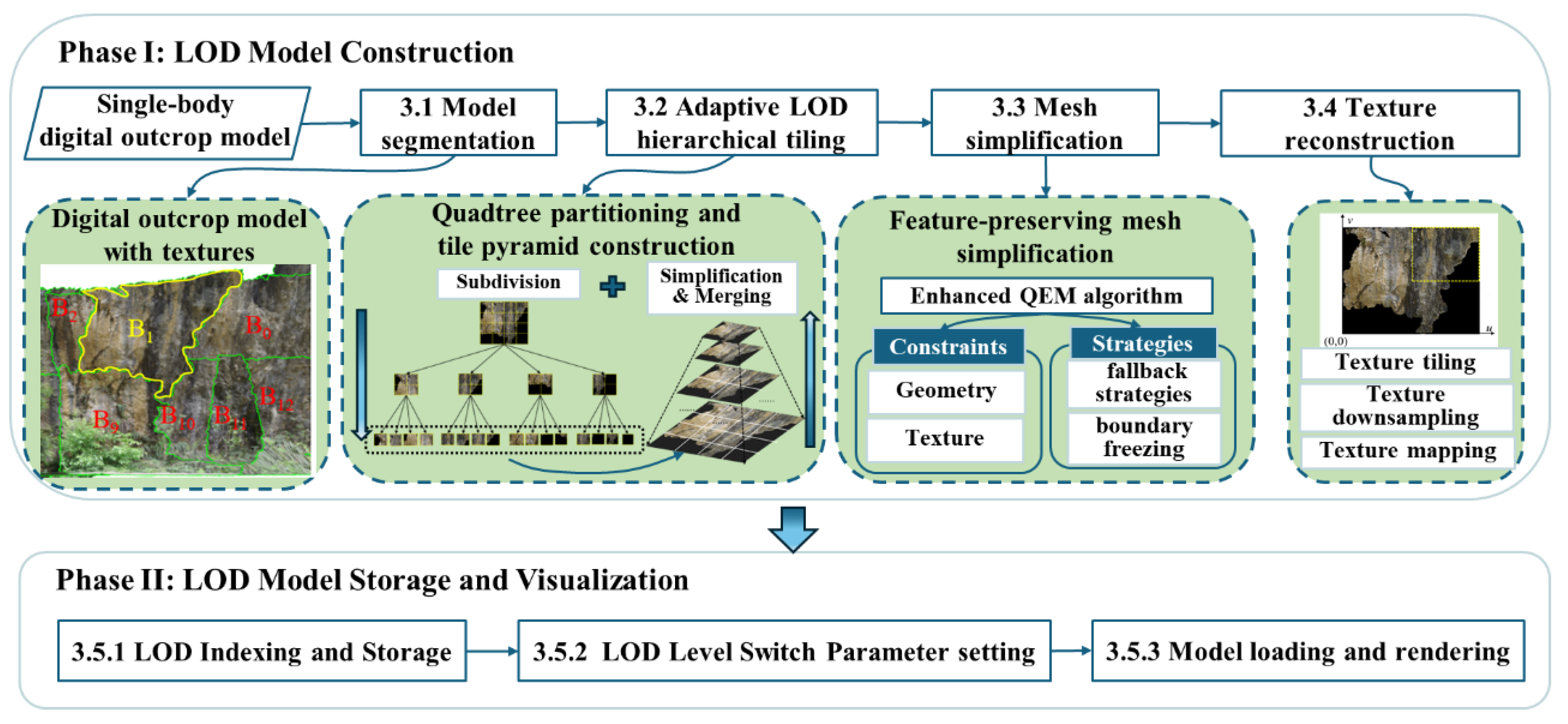
Figure 2.
Model partitioning into sub-models based on texture boundaries. (a) Digital outcrop model with texture boundaries in 3D space; (b) texture image of sub-model B1; and (c) projection of the triangular mesh corresponding to sub-model B1 in the 2D texture space.
Figure 2.
Model partitioning into sub-models based on texture boundaries. (a) Digital outcrop model with texture boundaries in 3D space; (b) texture image of sub-model B1; and (c) projection of the triangular mesh corresponding to sub-model B1 in the 2D texture space.
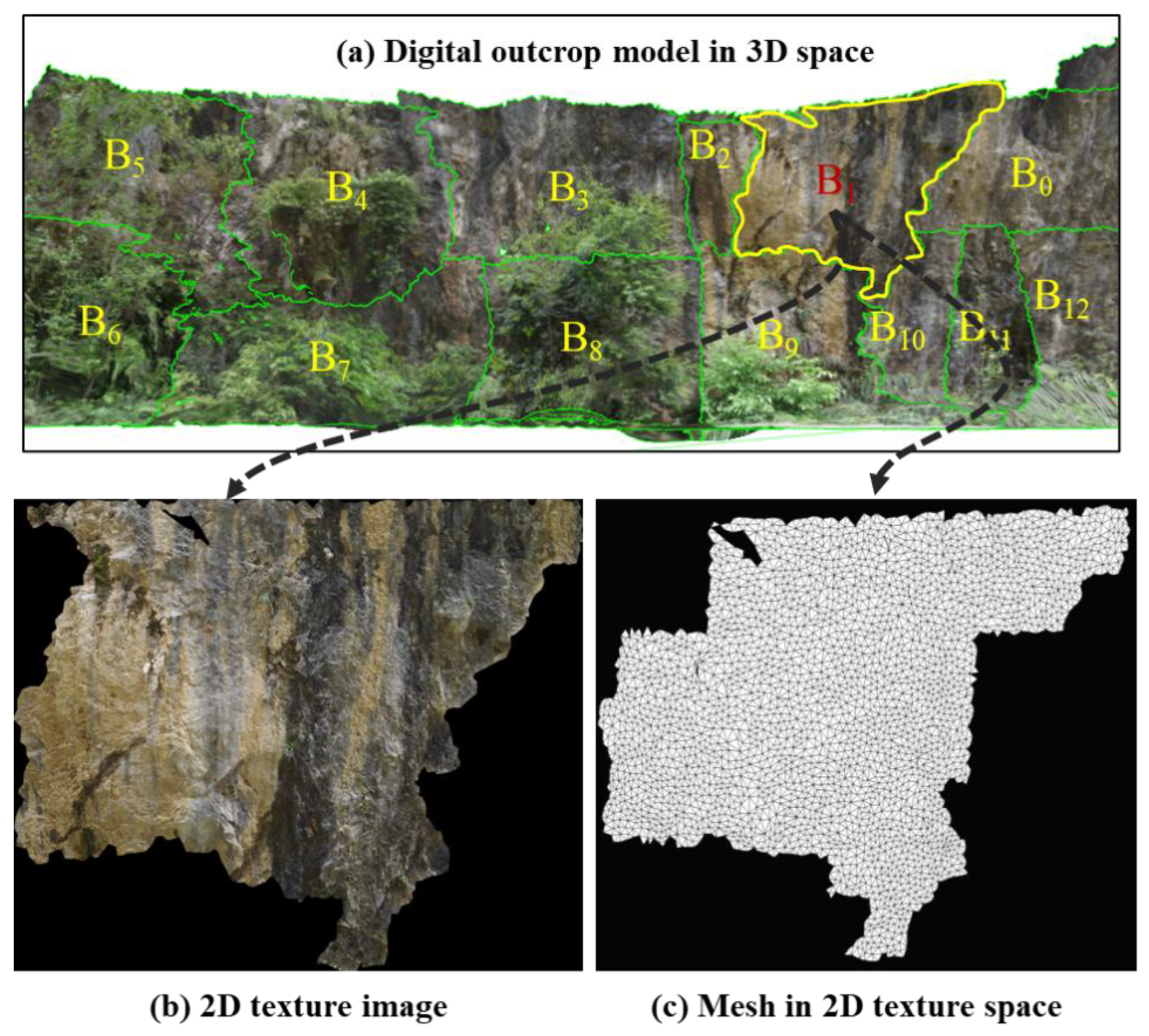
Figure 3.
Illustration of the quadtree subdivision process. Assuming a threshold of 1 MB and the original model size of 10 MB, it can be derived from Equation (1) that two quadtree subdivisions are required for the tile size to meet the threshold. (a) shows the texture image of a sub-model, and (b) shows the bottom-level tiles obtained after applying two quadtree subdivisions to this texture image, where the last tile is an invalid tile.
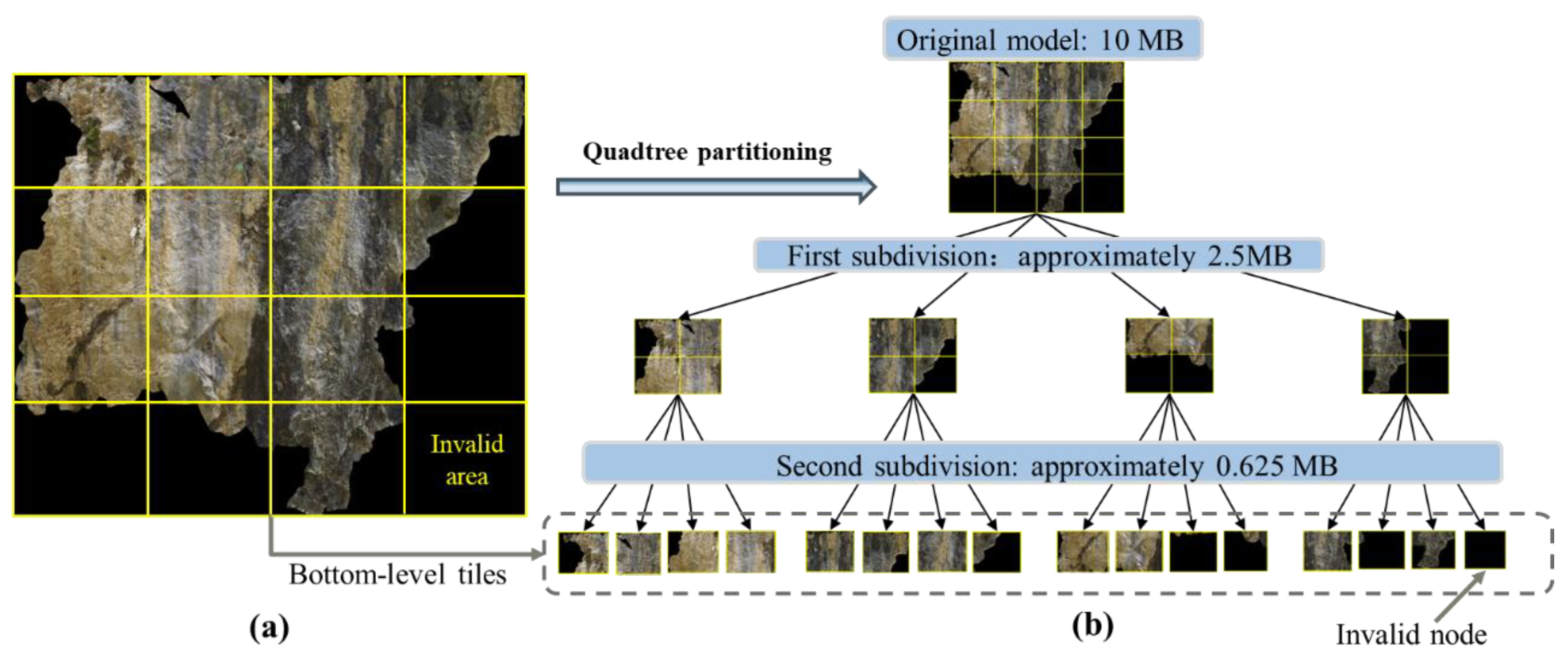
Figure 4.
Bottom-up tile simplification and merging. (a) and (b) illustrate the tiles simplification and merging process between adjacent two levels. Starting from the four tiles at level i (Nodei,0, Nodei,1, Nodei,2, Nodei,3), after simplification, the total data size at the upper level i−1 does not exceed the threshold Vt, these four tiles are merged into a single parent node, reflecting the bottom-up “simplify and merge” strategy. (c) and (d) show the processing across multiple levels. Starting from the level i, up through level i−1, level i−2, and so on, some levels are not merged due to data size constraints, while simplification continues. This process ultimately forms a multi-level LOD structure.
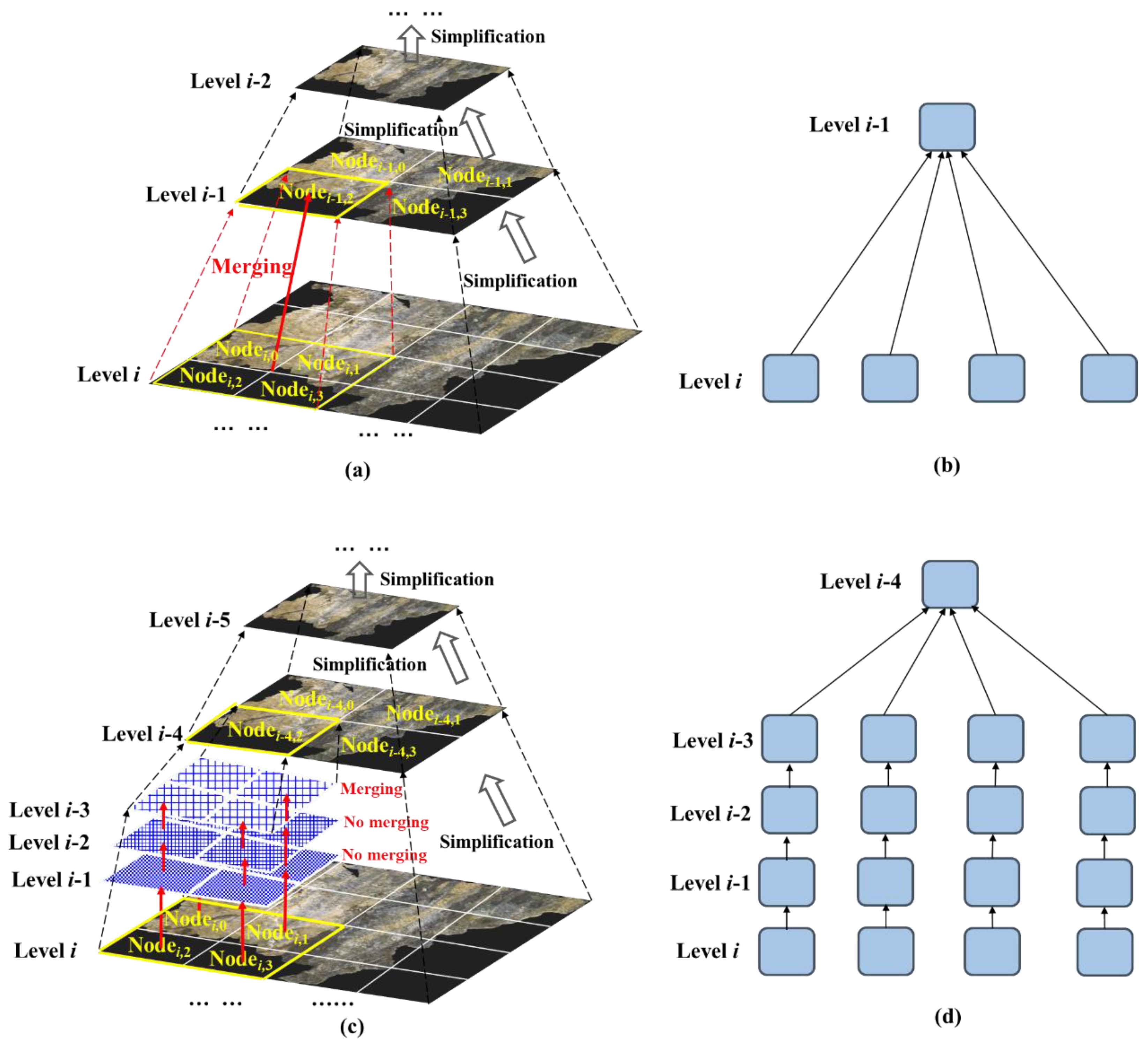
Figure 5.
Calculation of vertex sharpness. N1 and N2 are the normal vectors of the triangle planes.
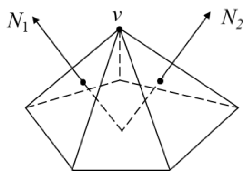
Figure 6.
Strategies for specific cases. (a) Strategy 1, (b) Strategy 2, (c) Strategy 3, and (d) Strategy 4.
Figure 6.
Strategies for specific cases. (a) Strategy 1, (b) Strategy 2, (c) Strategy 3, and (d) Strategy 4.
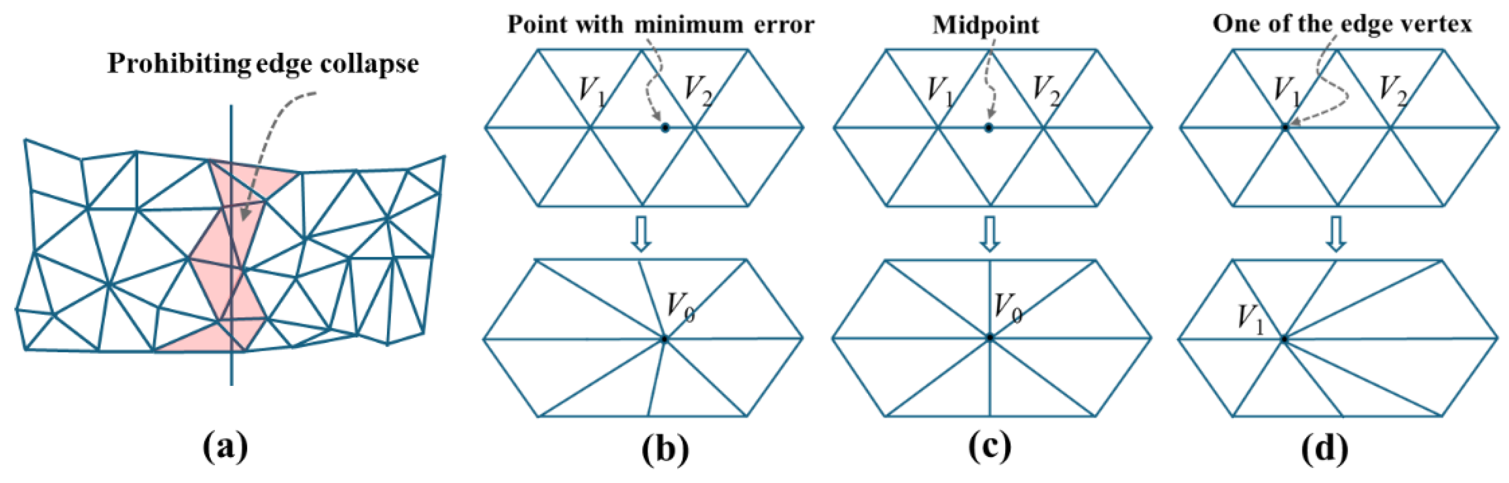
Figure 7.
Flowchart of edge-collapse decision strategies in the feature-preserving QEM simplification algorithm.
Figure 7.
Flowchart of edge-collapse decision strategies in the feature-preserving QEM simplification algorithm.
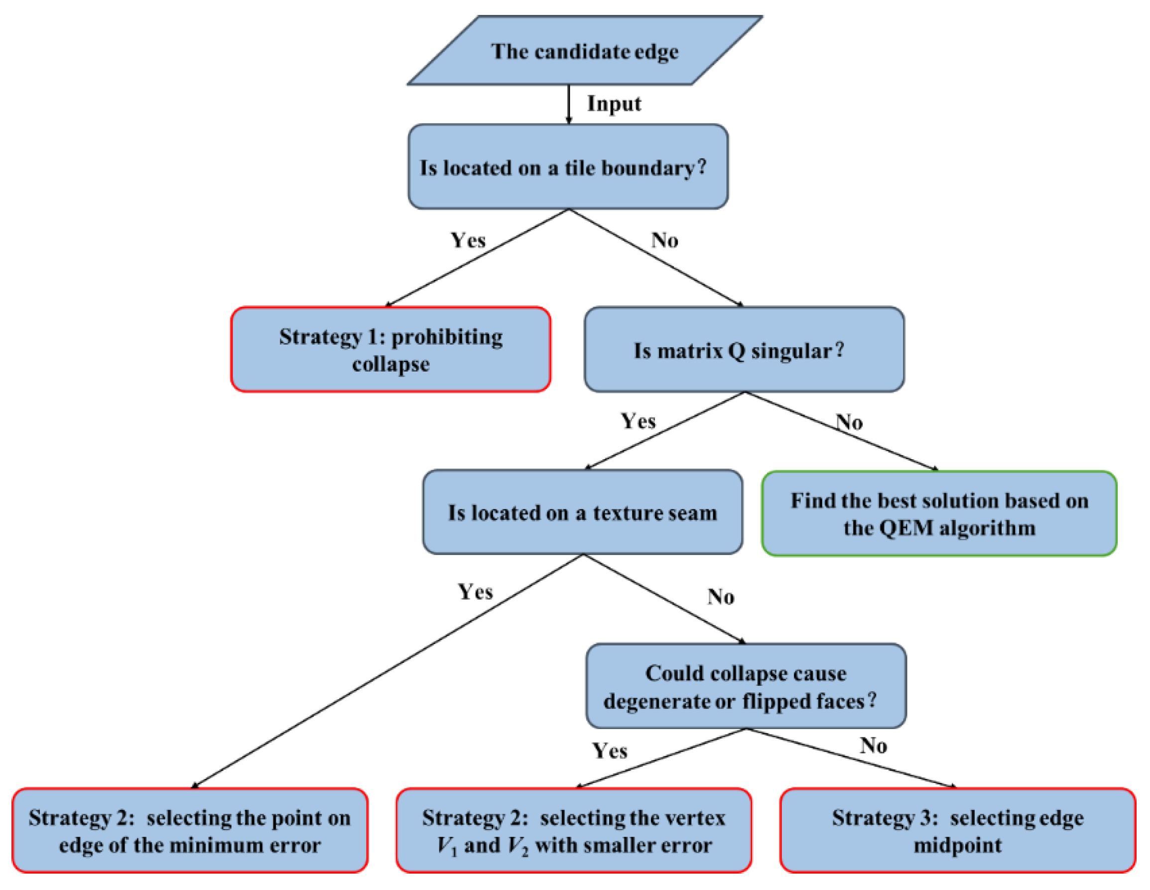
Figure 8.
Schematic illustration of texture downsampling and coordinate remapping for a single tile. The original global texture image is partitioned into rectangular tiles. For each tile, the corresponding texture region is cropped based on its coordinate extent (umin, vmin, umax, vmax). The cropped image is then downsampled to match the simplification ratio, and new texture coordinates are recalculated according to Equation (8) to ensure consistency between the simplified mesh and its local texture mapping.
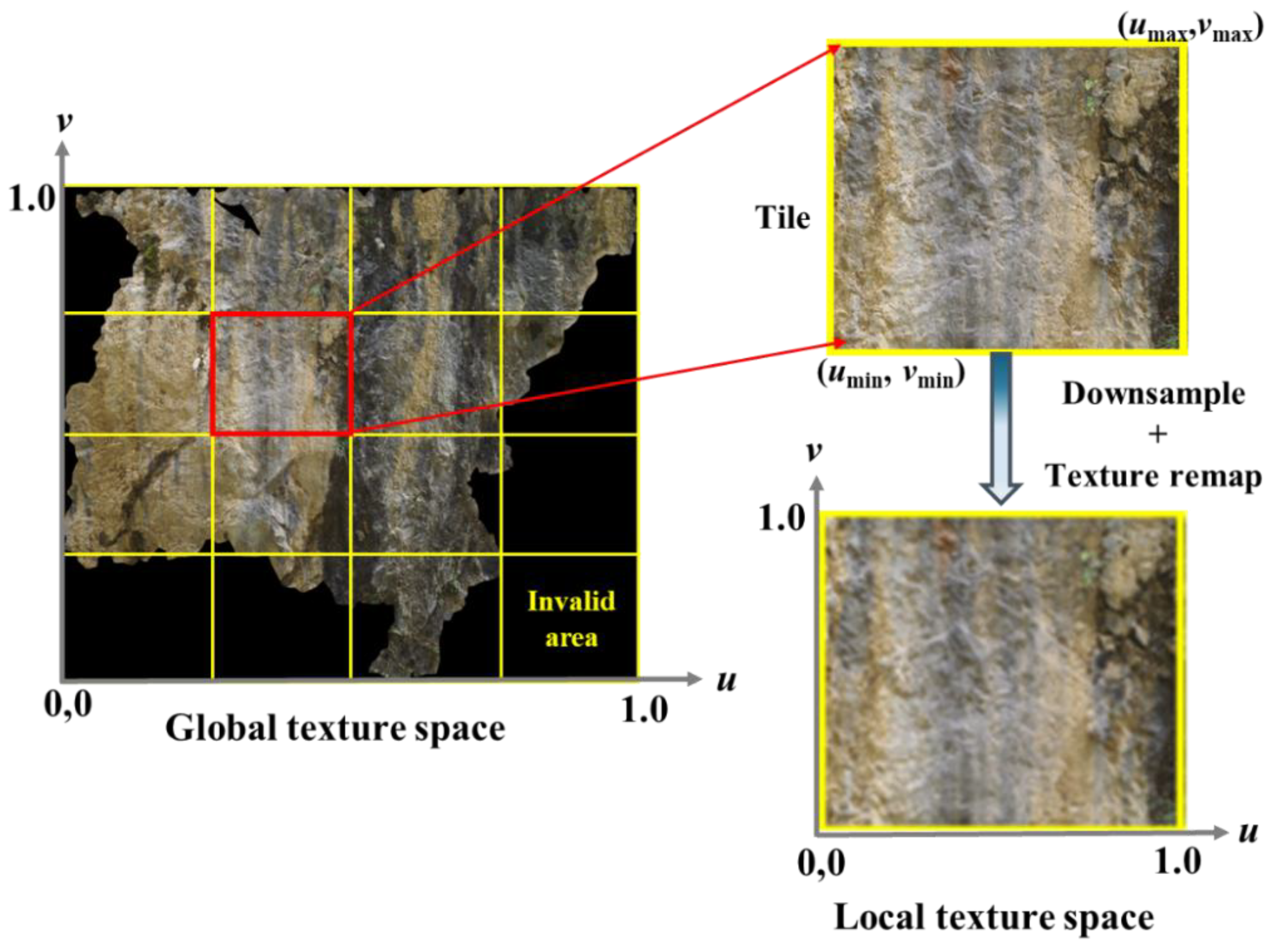
Figure 9.
Schematic diagram of the LOD grid indexing and tile pyramid organization. The entire LOD model is represented by the root node R (Level 0) and is partitioned into multiple rectangular grids G = {G₀, G₁, …, Gₖ₋₁} (Level 1). Each grid contains several sub-models, denoted as Level 2 nodes. For example, G₁ contains n sub-models, expressed G₁ = {B₀, B₁, …, Bₙ₋₁}. From Level 3 downward, each sub-model is further decomposed into a multi-scale tile pyramid. To efficiently organize these hierarchical nodes, a pseudo-quadtree spatial index is constructed, in which parent–child relationships can be either one-to-one or one-to-four. (a) Spatial partitioning and block-based LOD construction of the outcrop model. (b) Hierarchical organization of the grid index and tile pyramid for LOD management.
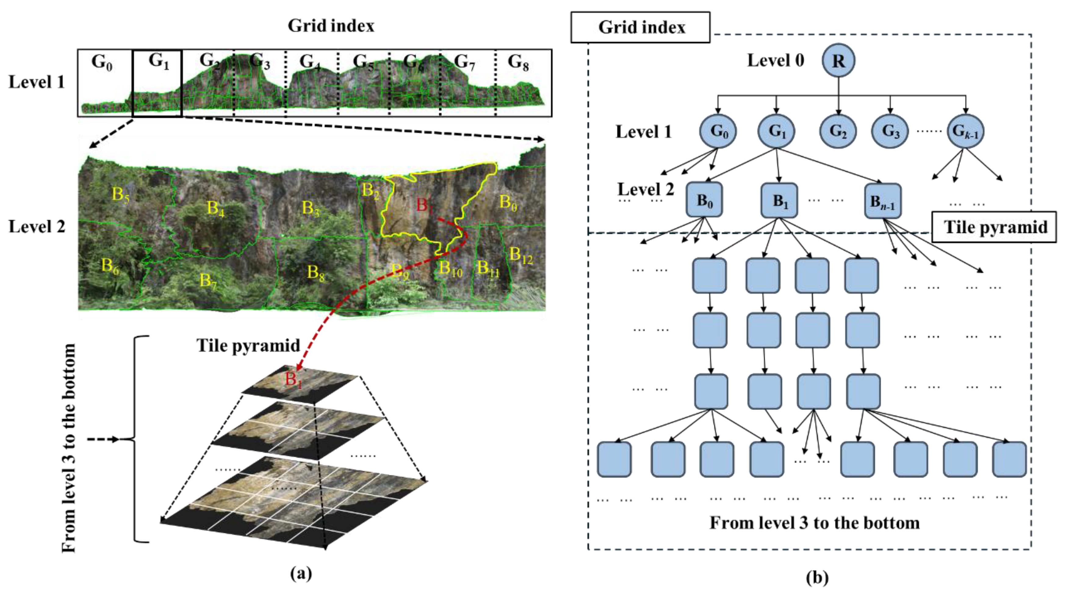
Figure 10.
Geometric illustration of screen-pixel–based LOD switching in OSG. (a) 3D view showing the camera frustum, viewport plane and the model bounding sphere; (b) 2D cross-section used for analytical estimation of the model’s projected size.
Figure 10.
Geometric illustration of screen-pixel–based LOD switching in OSG. (a) 3D view showing the camera frustum, viewport plane and the model bounding sphere; (b) 2D cross-section used for analytical estimation of the model’s projected size.
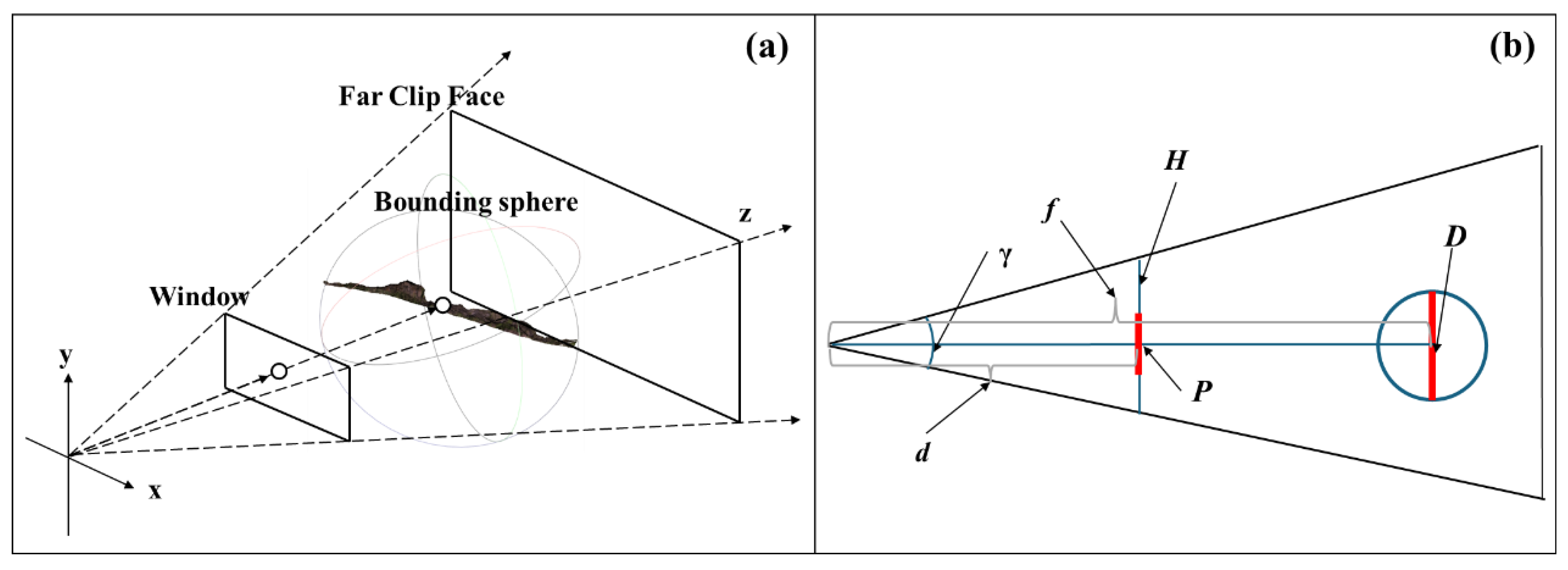
Figure 11.
LOD model loading and rendering based on the OSG engine.
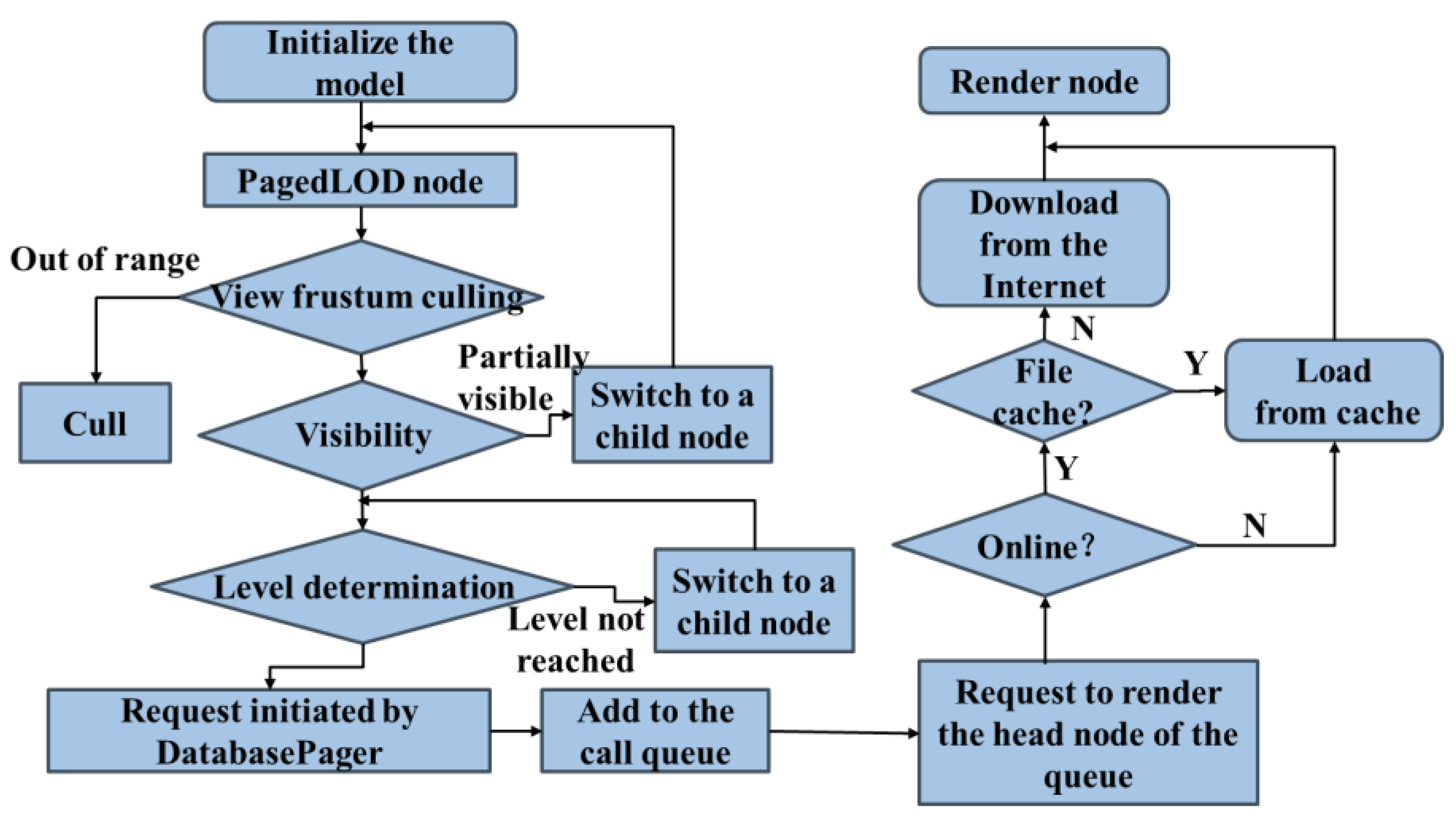
Figure 12.
Two constructed single-body LiDAR-derived outcrop digital models: (a) Model 1, (b) Model 2.
Figure 12.
Two constructed single-body LiDAR-derived outcrop digital models: (a) Model 1, (b) Model 2.
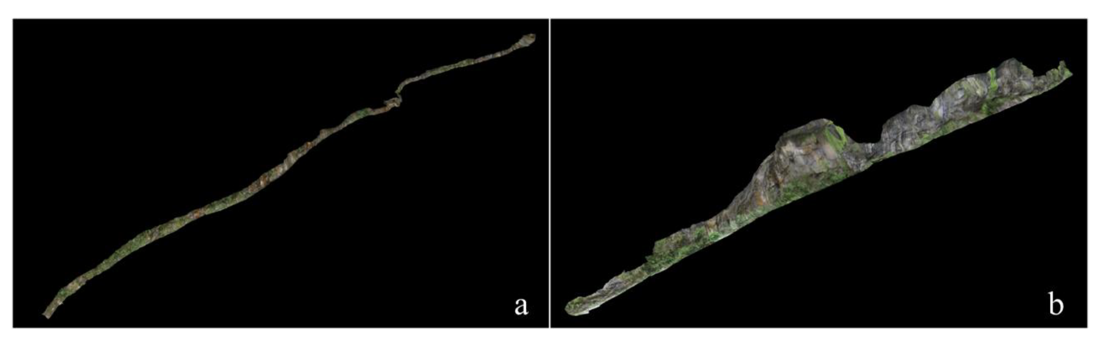
Figure 13.
Model rendering frame rate at different viewing distances: (a)model 1, and (b) model 2.
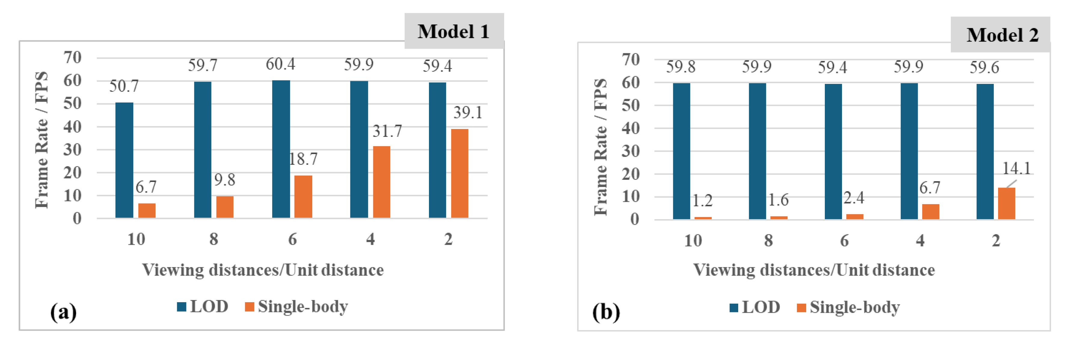
Figure 14.
Visualization of the LOD model 1 at different viewing distances: (a) Viewing distance of 10, (b) Viewing distance of 8, (c) Viewing distance of 6, (d) Viewing distance of 4 , (e) Viewing distance of 2.
Figure 14.
Visualization of the LOD model 1 at different viewing distances: (a) Viewing distance of 10, (b) Viewing distance of 8, (c) Viewing distance of 6, (d) Viewing distance of 4 , (e) Viewing distance of 2.
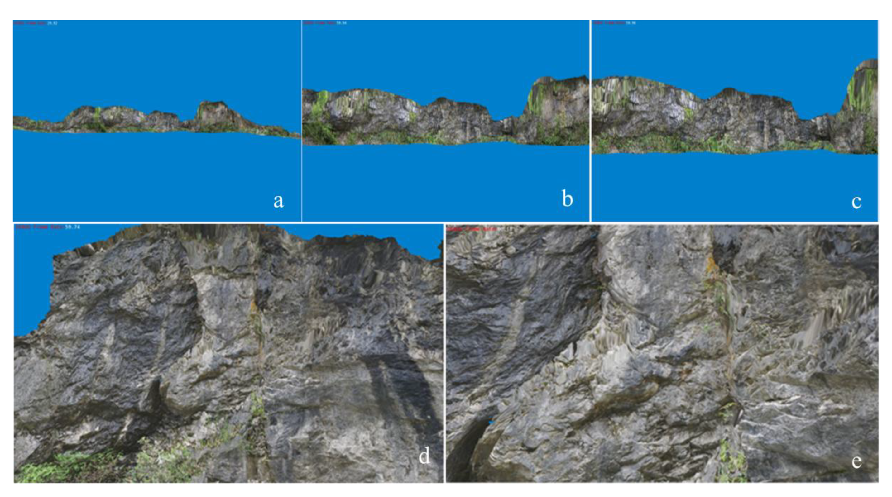
Figure 15.
Visualization of the LOD model 2 at different viewing distances: (a) Viewing distance of 10, (b) Viewing distance of 8, (c) Viewing distance of 6, (d) Viewing distance of 4 , (e) Viewing distance of 2.
Figure 15.
Visualization of the LOD model 2 at different viewing distances: (a) Viewing distance of 10, (b) Viewing distance of 8, (c) Viewing distance of 6, (d) Viewing distance of 4 , (e) Viewing distance of 2.
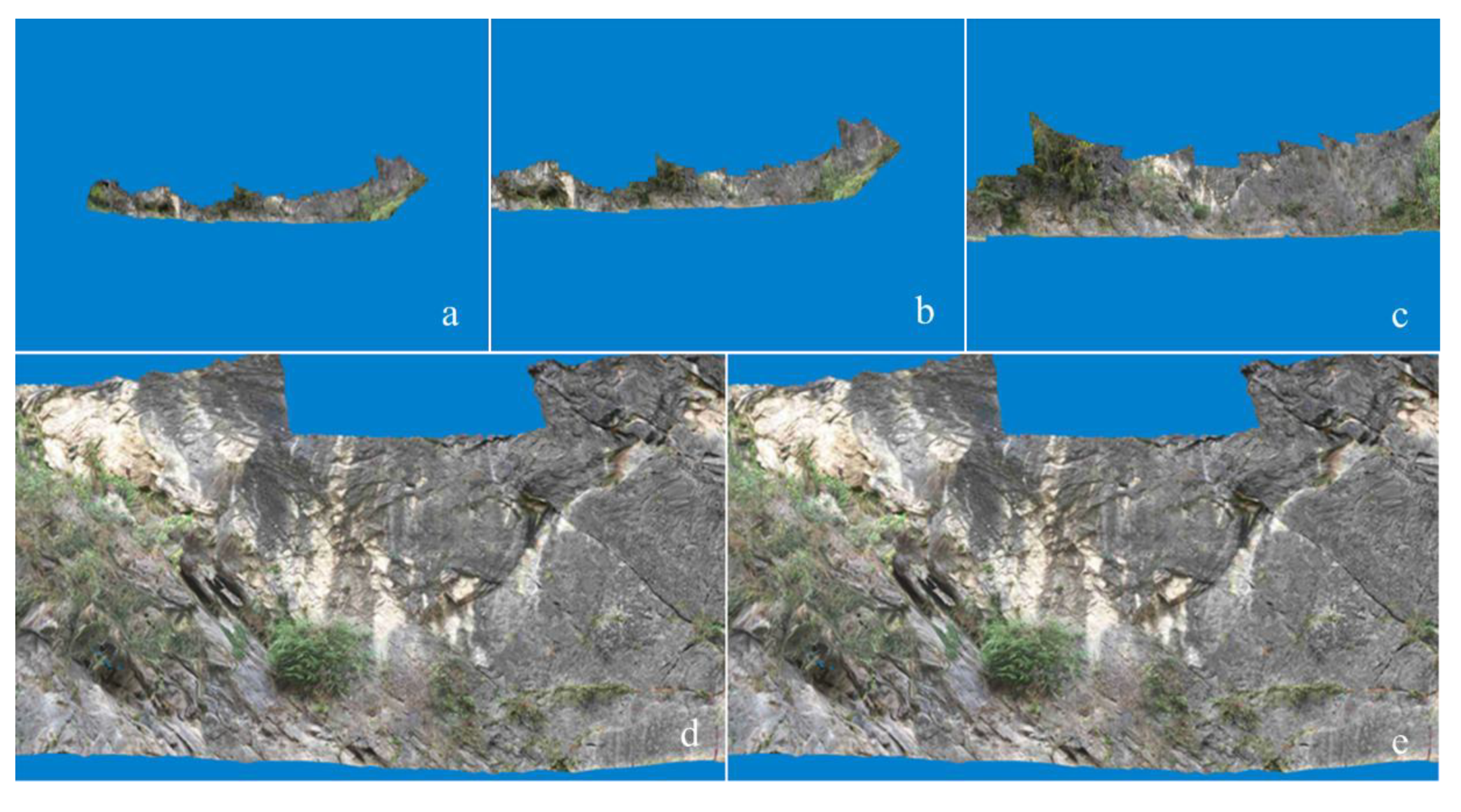
Figure 16.
Simplification error comparison for Model 2: (a) Geometric error comparison, (b) Texture error comparison.
Figure 16.
Simplification error comparison for Model 2: (a) Geometric error comparison, (b) Texture error comparison.
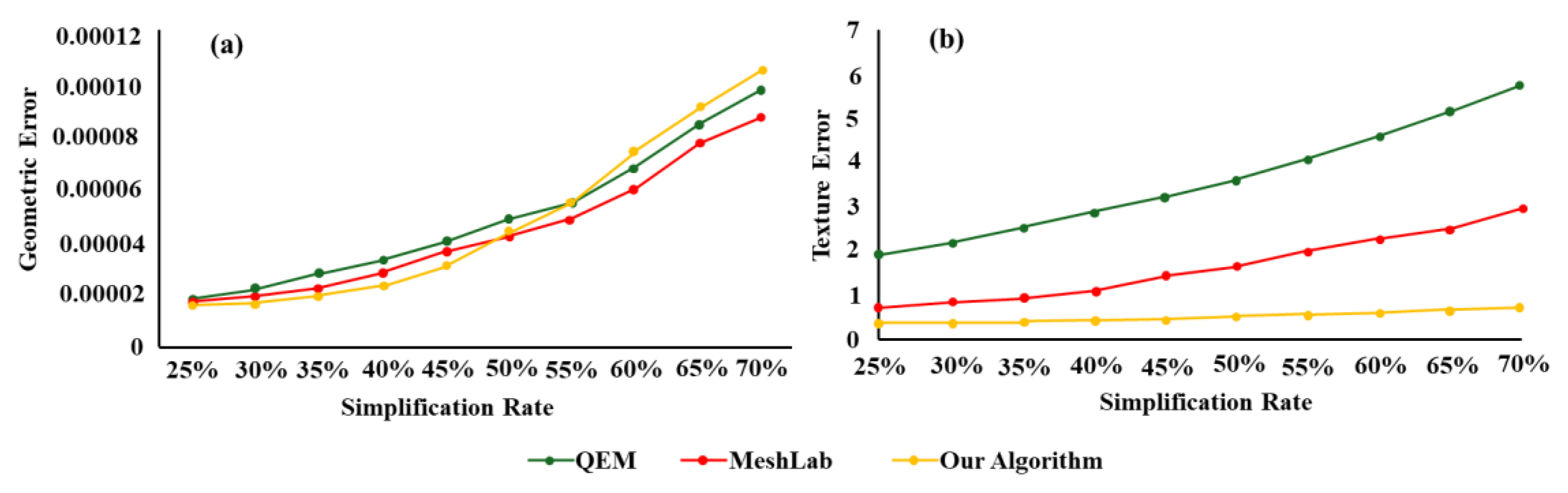
Figure 17.
Visual quality comparison of simplified Model 2.
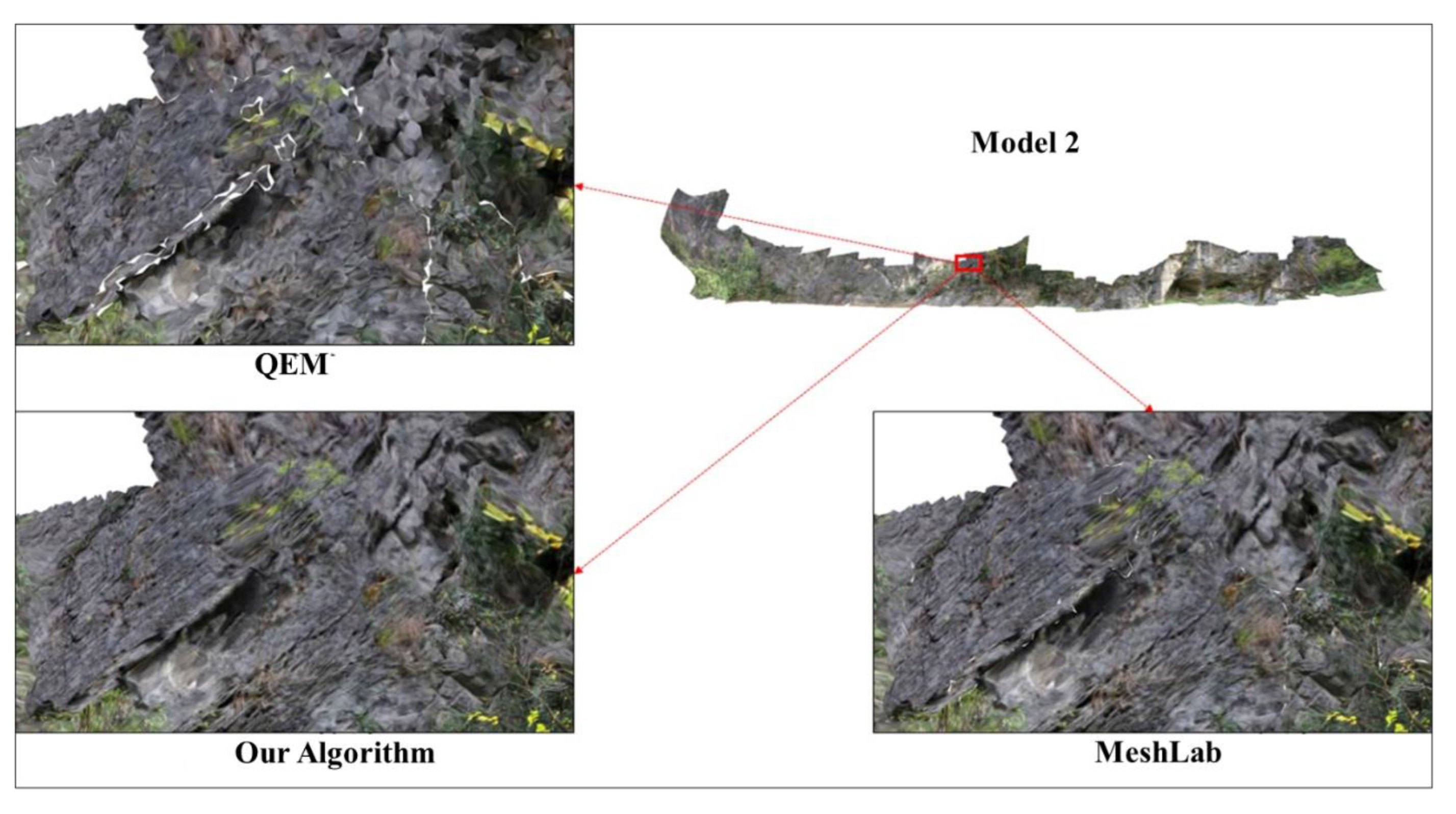

Table 1.
The basic information of the single-body digital outcrop models.
| Model | Number of vertices | Number of Triangular Facets | Number of Texture Images | Amount of the Model (GB) |
|---|---|---|---|---|
| Model 1 | 592473 | 1145853 | 103 | 1.16 |
| Model 2 | 648698 | 1244590 | 146 | 1.74 |
Table 2.
The basic information of the two LOD models.
| Model | execution time (s) | average memory usage (MB) | average CPU usage (%) | Amount of the LOD Model(GB) |
|---|---|---|---|---|
| Model 1 | 8424 | 2651.7 | 9.6% | 9.74 |
| Model 2 | 13,428 | 3352.7 | 11.6% | 8.72 |
Table 3.
LOD model loading test data.
| Model | Average CPU usage (%) | Average memory usage (MB) | Loading time (s) | Display frame rate (FPS) |
|---|---|---|---|---|
| Model 1 (LOD) | 15 | 188 | 3.7 | 50.7 |
| Model 1 (single-body) | 20 | 3506 | 117.5 | 6.7 |
| Model 2 (LOD) | 13.4 | 112 | 4.1 | 59.8 |
| Model 2 (single-body) | 20.2 | 11602 | 550.7 | 1.2 |
Disclaimer/Publisher’s Note: The statements, opinions and data contained in all publications are solely those of the individual author(s) and contributor(s) and not of MDPI and/or the editor(s). MDPI and/or the editor(s) disclaim responsibility for any injury to people or property resulting from any ideas, methods, instructions or products referred to in the content. |
© 2025 by the authors. Licensee MDPI, Basel, Switzerland. This article is an open access article distributed under the terms and conditions of the Creative Commons Attribution (CC BY) license (http://creativecommons.org/licenses/by/4.0/).
Copyright: This open access article is published under a Creative Commons CC BY 4.0 license, which permit the free download, distribution, and reuse, provided that the author and preprint are cited in any reuse.


