
Submitted:
19 September 2025
Posted:
06 October 2025
You are already at the latest version
Abstract
In this study, we consider and analyze inhomogeneous Whittaker-type differential equation of the form d2y(x)dx2+1xdy(x)dx−α2x2−β2y(x)=g(x), where α and β are given parameters. We investigate the analytical structure of its solution through the application of the Whittaker integral representation. The analysis encompasses both initial value problems (IVPs) and boundary value problems (BVPs), wherein appropriate conditions are imposed within a unified analytical framework. Furthermore, a systematic methodology is developed for constructing explicit solutions within the framework of Whittaker function theory. This approach not only elucidates the functional behaviour of the solutions but also provides a foundation for extending the analysis to more general classes of second-order linear differential equations.
Keywords:
Inhomogeneous Whittaker equations
; Whittaker functions
; integral Whittaker functions
; Bessel functions
; incomplete Gamma functions
; confluent hypergeometric functions
; Whittaker type differential equations
1. Introduction
A Whittaker-type differential equation refers to a class of ordinary and partial differential equations that, through suitable transformations of variables and/or dependent functions, can be reduced to the canonical form of the Whittaker differential equation. In the context of partial differential equations, such equations typically arise when the method of separation of variables is employed to construct solutions, particularly within the framework of mathematical physics and spectral theory. The Whittaker’s equation itself arises as a special case of the confluent hypergeometric equation and is given by:
where and are parameters. Equations reducible to this form are of significant interest due to their connections with special functions, quantum mechanics, and mathematical physics for more details e refer the reader to [1,2,3,4]. The transformation to Whittaker form often reveals underlying symmetries or allows the use of well-established analytical techniques and known solutions. In this work, we focus on a particular form of Whittaker-type differential equations that can be transformed into a standard Whittaker equation through suitable changes of variables or functions.
Our objective is twofold: first, to provide a clear and thorough exposition of the solution techniques applicable to Whittaker-type differential equations; and second, to highlight their practical significance by giving examples of the importance of Whittaker-type equations in heat conduction problems.It should be emphasized that all computations related to the solutions of both the initial and boundary value problems were performed using Maple.
The Whittaker differential equation plays a fundamental role in the theory of special functions and quantum mechanics. A notable application is its connection to the initial value problem of the heat equation, where the heat equation can be transformed into a Whittaker form. This relationship enables the use of Whittaker functions to describe heat propagation under certain conditions, highlighting the equation’s importance in both theoretical and applied mathematical physics [5] . A rigorous analysis of integral transforms related to the initial Whittaker heat problem was presented by [5], wherein the theory of reproducing kernels was employed to examine the structure and properties of the associated kernel functions. The inhomogeneous Whittaker equation has been analyzed in detail by Abu Zaytoon et al. [6]. A solution to the inhomogeneous Whittaker equation was obtained by introducing a special integral function, denoted by , which, for specific values of the parameters and , can be expressed in terms of other well-known special functions. In this work, we will use the solution provided in [6] for the inhomogeneous Whittaker’s equation to express a solution of the Whittaker-type equation of the form:
In the subsequent sections, we will discuss the solution methods for this equation, as well as the associated initial and boundary value problems.
2. Inhomogeneous Whittaker Equation
The inhomogeneous Whittaker equation is a second-order linear differential equation of the form:
where and are parameters, and is a known forcing term. A comprehensive analysis of the solution to this differential equation is presented in [6], where both initial and boundary value problems are considered. Abu-Zaytoon et al. [6] introduced an integral function, denoted by , to express the solution of the inhomogeneous Whittaker Equation (3). The function is evaluated for various parameter values, which, in certain cases, reduce it to well-known special functions, including Bessel functions, Gamma functions, incomplete Gamma functions, and error functions.
A general solution of the inhomogeneous Whittaker equation is given by [6]:
In Equation (4), the functions and denote the Whittaker functions, which constitute a fundamental set of solutions to the homogeneous Whittaker Equation (1), (c.f. [7]). The function is defined as follows [6]:
where,
The derivatives of the Whittaker functions are given in [7] as:
Furthermore, the derivative of the function is given by [6]:
3. Whittaker Type Differential Equation
In the subsequent sections, we will demonstrate that Equation (2) belongs to the class of Whittaker-type differential equations. Through a series of appropriate transformations and analytical steps, we will show how it can be recast into the canonical form of the Whittaker’s differential equation.
To solve Equation (2), the next step involves applying an appropriate transformation that demonstrates its equivalence to the inhomogeneous Whittaker equation. We begin by introducing the following transformation:
Upon substituting the transformation into Equation (2), we obtain the following equation:
Equation (11) is an inhomogeneous Whittaker equation, where:
Utilizing Equation (5), the solution to Equation (11) is expressed as follows:
Finally, the solution to Equation (2) can be expressed in the form:
In the case where , the Whittaker functions can be expressed in terms of confluent hypergeometric functions; specifically, reduces to the confluent hypergeometric function of the first kind , and corresponds to the confluent hypergeometric function of the second kind , commonly known as Tricomi’s function [7], as follows:
The function admits the following integral representation, valid for (see [7]):
An expansion of the function yields a representation of that is particularly effective for analyzing the behaviour of the function in the regime of small x [7]:
where denotes the Pochhammer’s Symbol, and is the digamma function defined by:
When the parameters and satisfy the inequality , the function admits the following integral representation for [7]:
Notably, the function satisfies , indicating that it vanishes at the origin; further details can be found in [5]. Further research is warranted to derive closed-form expressions for the functions and , which may, in turn, facilitate the explicit representation of the associated -functions. Such developments would obviate the need for computational evaluation of Whittaker integral functions, thereby enhancing both the analytical tractability and efficiency of the solution process.
4. Initial and Boundary Value Problems
To advance toward the resolution of initial and boundary value problems involving Equation (2), it is necessary-particularly in the context of initial value problems-to determine the derivative of the the solution . By differentiating both sides of Equation (13), we obtain the following expression for :
Upon substituting Equations (7), (8), and (9) into Equation (21), we obtain the following:
4.1. Initial Value Problems
Consider the inhomogeneous Whittaker-type differential equation given in Equation (2), subject to the following initial conditions:
To solve the initial value problem, we start by substituting the initial conditions from (23) into Equations (13) and (24), yielding:
which can be rewritten in matrix form as:
where
upon solving the system we get:
and
Having established the general analysis, we proceed to exemplify the solution of initial value problems governed by Equation (2). An illustrative case is defined by the parameters and , coupled with the initial conditions
The solutions to this initial value problem, corresponding to distinct definitions of the source term , are computationally derived and plotted in Figure 1. In Figure 2, solution is presented for , and various values of . The effect of on the solution is shown in Figure 3 for , and different values of .
4.2. Boundary Value Problem
In this section, we introduce the boundary value problems associated with Equation (2), corresponding to the following boundary conditions:
We will start by applying the boundary condition (30) to Equation (13) in order to obtain:
which can be re writen in matrix form as:
where
upon solving the system we get:
and
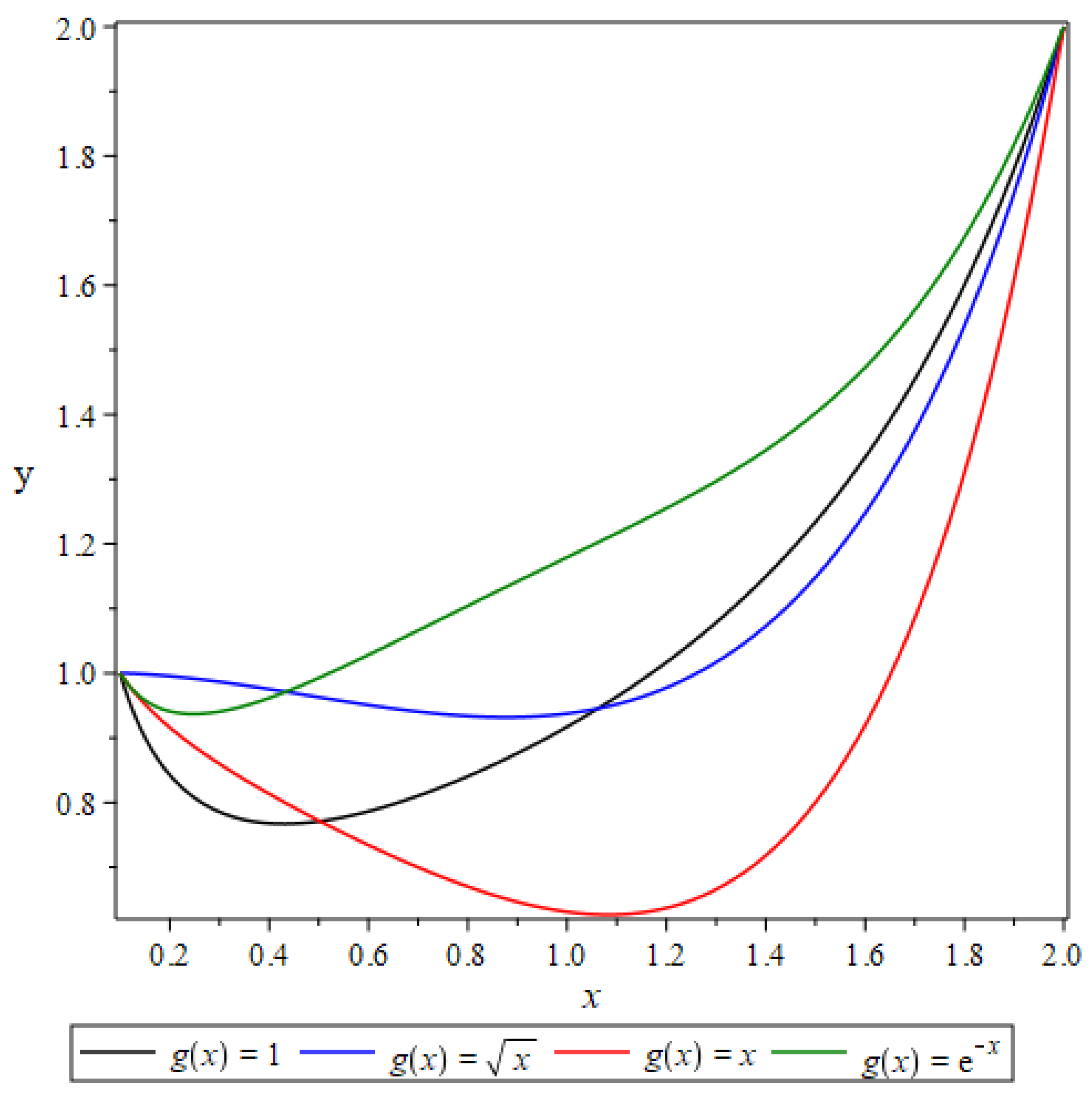
Solutions corresponding to various functions and boundary conditions and are shown in Figure 4, whereas the solutions for boundary conditions y(0.1)=1 and y(2)=2 are depicted i in Figure 5.
5. Conclusions
The principal objective of this work is to present a solution to a class of Whittaker-type differential equations, specifically those of the form given in Equation (2). Both initial value problems (IVPs) and boundary value problems (BVPs) are considered within this framework. The analytical approach employed is based on the function , as introduced in [6]. Graphical representations of the solutions are provided for selected parameter values and corresponding external forcing functions generated using Maple. The method developed herein contributes to the broader study of inhomogeneous Whittaker-type differential equations. While the current work emphasizes computational solutions, a more in-depth analytical investigation could yield closed form expressions for the function , particularly in the special case where . The methodology developed in this work is not restricted to the specific differential equation under consideration; it also proves effective in deriving solutions to a broader class of Whittaker-type differential equations. Moreover, it may be extended to certain partial differential equations that can be reduced to Whittaker-type forms via separation of variables or appropriate transformations of variables.
Author Contributions
M.A.Z prepared the first draft of the manuscript and generated the figures. H. A reviewed the initial draft and provided suggestions to improve the document. M. H reviewed the final draft of the manuscript and contributed recommendations to enhance the quality of the research. All authors have read and agreed to the published version of the manuscript.
Funding
This research received no external funding.
Data Availability Statement
No data were generated or analyzed in this study. All computations were performed symbolically using Maple.
Conflicts of Interest
The authors declare no conflicts of interest.
References
- Whittaker, E. An expression of certain known functions as generalized hypergeometric functions. Bull. Am. Math. Soc. 1903, 10, 125–134. [Google Scholar] [CrossRef]
- Abramowitz, M.; Stegun, I.A. Handbook of Mathematical Functions; Dover: New York, 1984. [Google Scholar]
- Magnus, W.; Oberhettinger, F.; Soni, R. Formulas and Theorems for the Special Functions of Mathematical Physics, 3rd ed.; Springer: Berlin, Germany, 1966. [Google Scholar]
- Hochstadt, H. The Functions of Mathematical Physics; John Wiley & Sons, Inc.: New York, NY, 1971. [Google Scholar]
- Rodrigues, M.M.; Saitoh, S. Whittaker Differential Equation Associated to the Initial Heat Problem. In Proceedings of the Current Trends in Analysis and Its Applications, Cham, Switzerland; 2015. [Google Scholar]
- Abu Zaytoon, M.S.; Al Ali, H.; Hamdan, M.H. Inhomogeneous Whittaker Equation with Initial and Boundary Conditions. Mathematics 2025, 13, 2770. [Google Scholar] [CrossRef]
- Olver, F.; Lozier, D.; Boisvert, R.; Clark, C. NIST Handbook of Mathematical Functions; Cambridge University Press: Cambridge, UK, 2010. [Google Scholar]
Figure 1.
Solution of for different values of
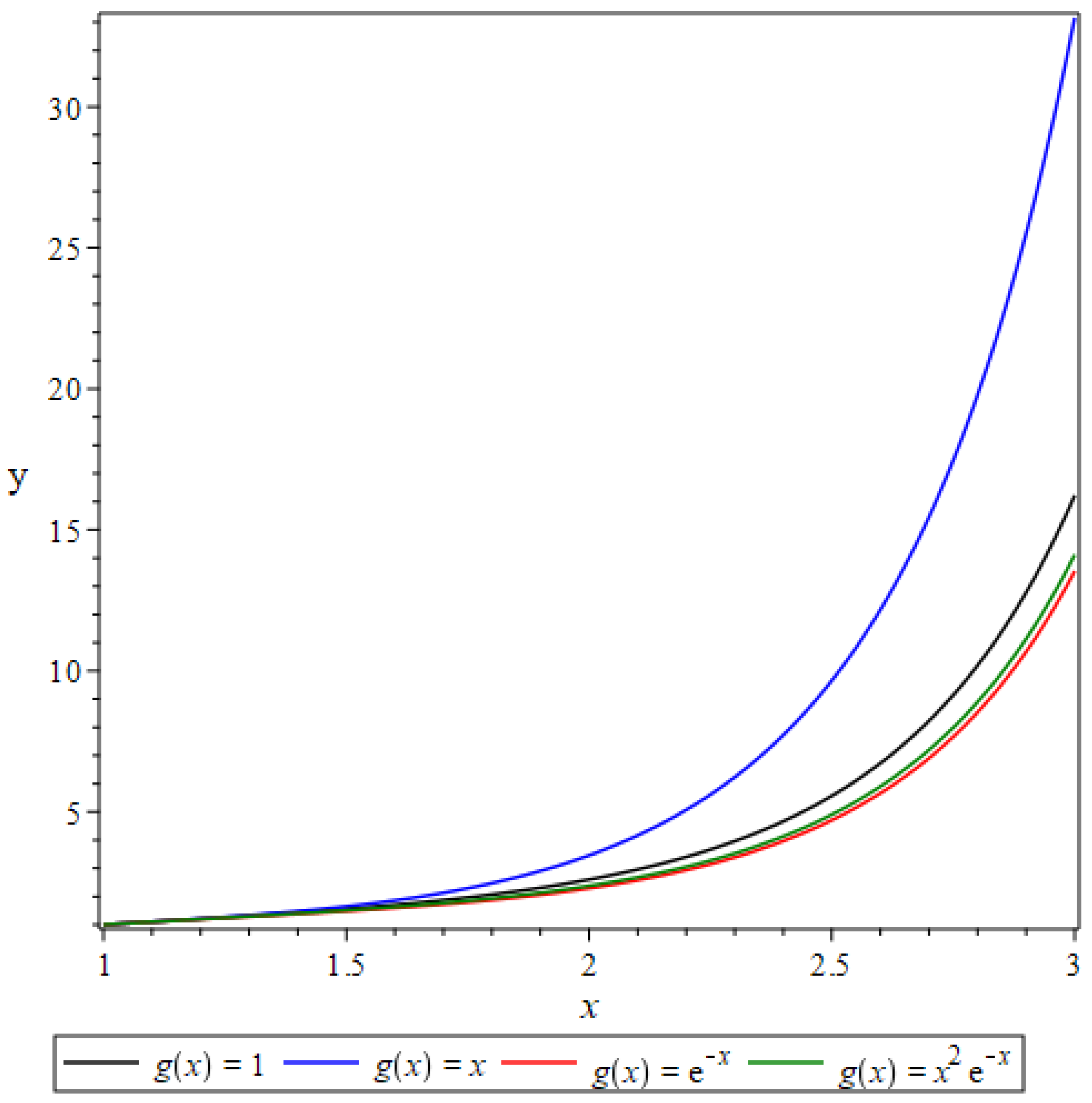
Figure 2.
Solution of for different values of

Figure 3.
Solution of for different values of
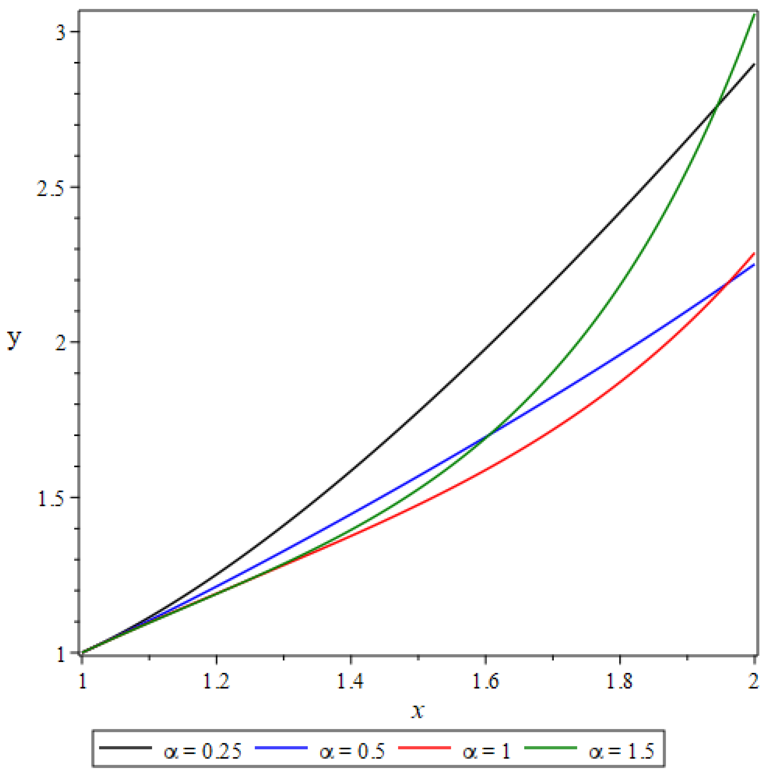
Figure 4.
Solution of for different
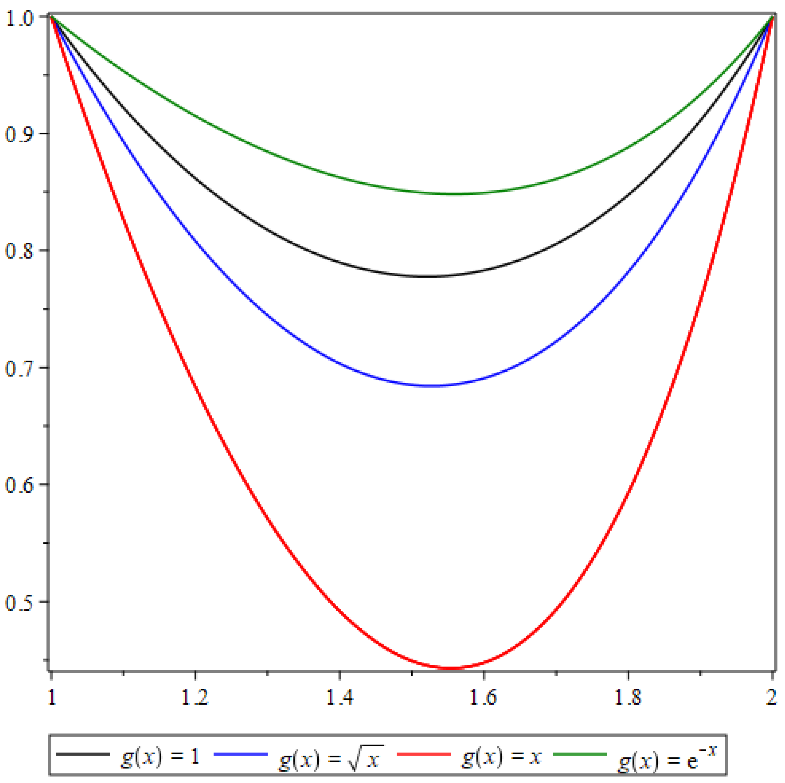
Figure 5.
Solution of for different
Disclaimer/Publisher’s Note: The statements, opinions and data contained in all publications are solely those of the individual author(s) and contributor(s) and not of MDPI and/or the editor(s). MDPI and/or the editor(s) disclaim responsibility for any injury to people or property resulting from any ideas, methods, instructions or products referred to in the content. |
© 2025 by the authors. Licensee MDPI, Basel, Switzerland. This article is an open access article distributed under the terms and conditions of the Creative Commons Attribution (CC BY) license (http://creativecommons.org/licenses/by/4.0/).
Copyright: This open access article is published under a Creative Commons CC BY 4.0 license, which permit the free download, distribution, and reuse, provided that the author and preprint are cited in any reuse.


