
Submitted:
02 October 2025
Posted:
02 October 2025
You are already at the latest version
Abstract
Understanding household energy demand patterns is essential for effective energy system planning and policy design. Building on previous cluster analysis of common daily demand profiles, this study identifies household electricity and gas ‘demand archetypes’ which capture the typical summer and winter weekday demand profiles for each home using modal daily demand profiles. We apply logistic regression with household survey data to identify potential explanatory factors. Our study uses half-hourly smart meter data from the Smart Energy Research Lab Observatory in Great Britain between November 2021 and August 2022; 9844 households with electricity data and 7251 with gas data after filtering. We find that household gas demand archetypes show much greater variability between seasons than electricity archetypes, consistent with seasonal variations in gas heating needs. Household demand archetypes with a morning and/or evening peak are the most prevalent in both seasons for electricity and gas. However, a substantial share of households exhibits highly variable demand profiles in both seasons, indicating inconsistent and possibly flexible routines. Logistic regression analysis reveals strong correlations between microgeneration and a midday trough in electricity demand, while electric vehicle ownership increases the likelihood of a variable demand profile. Financial wellbeing and family structure also show correlations with demand archetypes, with lower-income households more likely to exhibit variable and peak-time gas archetypes; perhaps indicating efforts to reduce costs. Our findings highlight the value of analysing household electricity and gas demand archetypes for different seasons and offer important insights for demand-side energy management, forecasting and policy.
Keywords:
Demand profiles
; household demand archetypes
; electricity data
; gas data
; energy consumption
; energy demand
; smart meter data
Highlights
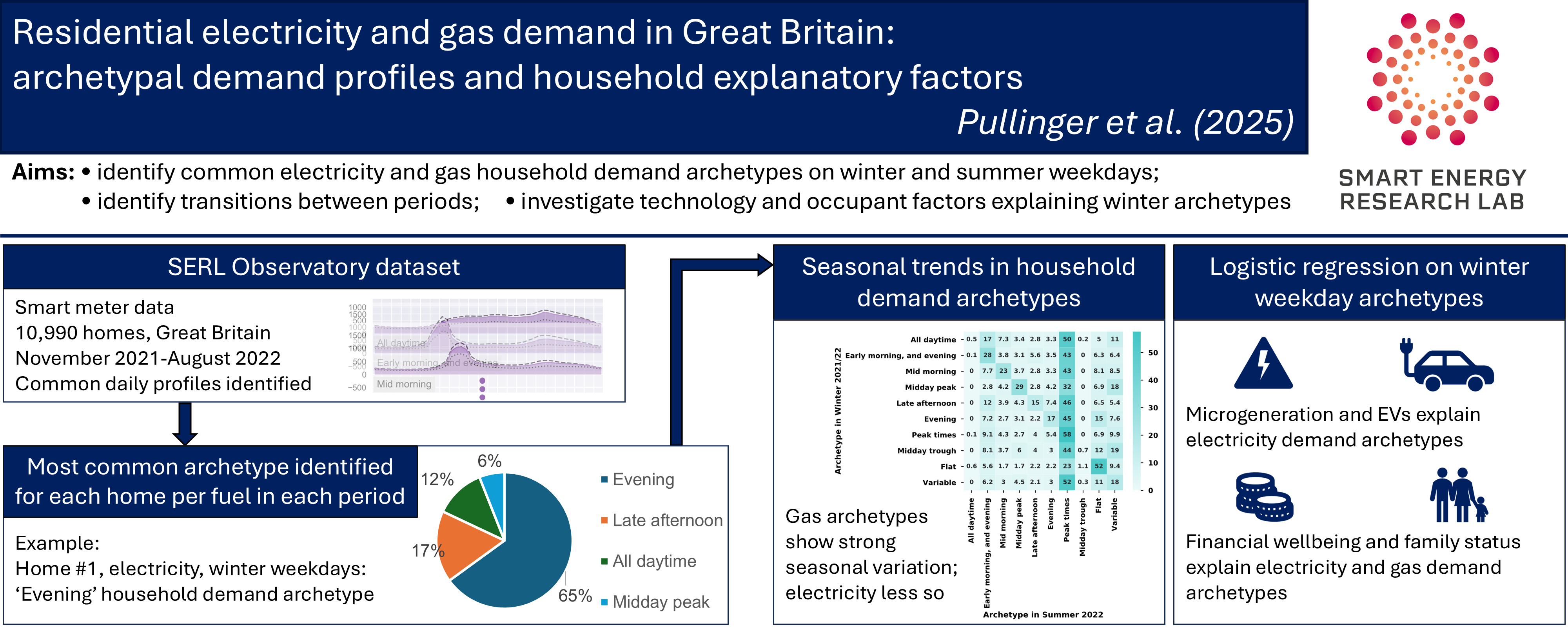
• Identifies GB household net electricity and gas demand archetypes post-COVID-19
• Uses modal daily profiles to define household archetypes for winter/summer weekdays
• Gas demand archetypes show strong seasonal variation; electricity less so
• Microgeneration and EVs explain electricity demand archetypes
• Financial wellbeing and family status explain electricity and gas demand archetypes
1. Introduction
Residential electricity and gas demand can vary substantially over the course of a day, from one day to the next, and between households. Daily demand profiles – the patterns of change in demand over the day, including the timings of peaks and troughs in demand – may be driven by the characteristics of the building, appliances and occupants, and shaped by time-varying factors such as sleeping-, working- and eating-patterns, weather conditions, changing seasons, and fuel price signals. Identifying a household’s typical electricity or gas daily demand profile from empirical data can improve modelling and forecasting of daily grid energy demand patterns, enable targeted demand-side management strategies, support the design of time-of-use tariffs, and facilitate the segmentation of households for energy policy interventions [1,2,3]. With ongoing changes in demand associated with post-pandemic working patterns and consumer reactions to energy price rises [4,5], as well as the impacts of decarbonisation efforts, improved analysis of daily demand profiles is therefore vital for policy makers, energy suppliers, and grid operators to better understand the energy requirements of different types of consumers.
Fortunately, the rollout of smart meters in many countries – devices that transmit energy (or water) usage data offsite to end users, typically at an hourly or minute-level resolution – provides a rich new data source to investigate demand profiles. Indeed, an increasing number of research studies draw on such data to identify demand ‘archetypes’ – typical profiles that are found to be common across a set of homes and over time – and to investigate which factors explain or predict what archetype a home will exhibit for a particular day, or on average over a period of time. These studies draw on data from a range of countries and time periods, and have investigated, among other things: the influence of different methodological approaches, notably different forms of cluster analysis, on the number and shape of the demand archetypes that are identified [1,6,7,8]; household-level factors (e.g. building type, heating system, number of occupants) and temporally-varying factors (e.g. external temperature, day of week, pandemics) that explain or predict a particular home’s demand archetype [9,10,11,12]; and the contributions that identifying common demand archetypes might make to improving demand-side response programmes [13] and load forecasting methods [14,15].
In our previous work [16], we focused on the influence of time-varying factors on the daily demand archetypes of the full sample. In this paper, we investigate static household-level factors that explain individual household demand archetypes for winter and summer weekdays.
There are several gaps in the existing literature that this study aims to address. Many existing studies make use of static datasets that predate the COVID-19 pandemic, and therefore do not capture the substantial changes in home working patterns that occurred during that period, and which are a major driver of occupancy-related demand [16,17]. The large majority of studies relate to electricity demand archetypes only. We have only identified one other research group that has investigated gas demand archetypes [10,11]. Only one was identified that has published work on both electricity and gas from the same homes, and with post-pandemic data [18] (using the same dataset as in this study). Unlike that study, which combined data from both fuels to produce a single demand archetype per home for a full year, we identify separate demand archetypes per fuel and for separate periods of the year.
The current study therefore has two research aims to contribute to the current body of work in this area:
1. Identify common household demand archetypes for households in Great Britain using post-covid-pandemic household smart meter data (primarily from 30 November 2021 to 31 August 2022) for both electricity and gas demand. In keeping with existing literature, we focus on specific periods of time to control for variation in weather and societal drivers of demand, specifically winter weekdays and summer weekdays (see Glossary above).
2. Investigate how a household’s demand archetype is related to its technology and occupant characteristics. As residential energy demand in GB is highest in the heating season, we focus on their energy demand archetypes over the winter period (specifically winter weekdays). We investigate the relationship of these archetypes to a range of technology and occupant characteristics, namely the household’s primary heating fuel, presence of microgeneration (such as rooftop solar photovoltaic (PV) panels), electric vehicle (EV) ownership, family status (presence of workers and school-age children), and financial wellbeing.
The paper addresses the above aims through answering two research questions:
1. What is the prevalence of each household demand archetype on winter weekdays and summer weekdays, and what transitions between demand archetypes are most common for households to make between these two periods?
2. What (if any) technology and occupant factors explain a household’s demand archetype on winter weekdays?
The current study utilises data from the Smart Energy Research Lab (SERL) Observatory dataset, which includes half-hourly electricity and gas smart meter data from a sample of 13,000+ consenting households that are a broadly representative sample of the Great Britain (GB) population, along with linked survey data on household characteristics [19,20,21,22]. This is combined with data on daily electricity and gas demand archetypes for each day between 1 September 2020 to 31 August 2022, developed using cluster analysis of the smart meter data and presented in our previously published work [16].
The paper takes the following structure: Section 2 provides a review of related literature. Section 3 describes the datasets used in this study: the SERL Observatory and the daily demand archetypes derived from it. Section 4 describes the methodology used to generate household demand archetypes from the daily demand archetypes, and to investigate factors explaining a household’s demand archetype. Section 5 presents results, describing the prevalence of the household demand archetypes for the selected winter weekday and summer weekday periods, and presenting an analysis of the household-level factors which explain them. Section 0 discusses the implications of the results and considers the limitations of the current work and possibilities for future research. Section 7 provides the key conclusions.
2. Literature Review
Research applying cluster analysis to residential energy demand profiles is largely split into two broad approaches. The first treats each daily demand profile from each home as a separate case for the cluster analysis, so that for each home, each day has its own daily demand archetype attributed to it. Daily demand archetypes may therefore vary from day to day for a given home, as well as vary between homes on any given day. This approach is particularly suited to analysing how demand archetypes change with time-varying factors, and was the approach used in our previous work [16], in which we treated electricity and gas profiles from each home and day as separate cases, and which analysed how demand patterns changed over time, particularly in relation to levels of lockdown during the COVID-19 pandemic and to external temperature.
In the second type of analysis, the average demand profile over a period of time for each home is taken as the unit of analysis. Identifying a household’s energy demand archetype over, for example, a full winter, can help to see the home’s underlying typical pattern of demand under those conditions. This can therefore facilitate analyses of the influence of household characteristics on household demand archetypes, in effect by smoothing out day-to-day variations driven by weather or other external factors.
For simplicity, we refer to the cluster results arising from these two levels of analysis as daily demand archetypes and household demand archetypes (the latter being the focus of this paper; see Glossary). Household demand archetypes are the focus of the current study and thus also the focus of the literature review presented here, which we also restrict to studies with an applied focus and/or that use datasets of a similar scale to ours - specifically, with at least one year of data for at least 1000 households.
2.1. Applications of Household Demand Archetype Analyses
The existing literature on household demand archetypes suggests several practical end uses. Satre-Meloy et al [23] reviewed various papers investigating household demand archetypes, many of which included analyses of how the identified archetypes correlated with a household’s dwelling and other characteristics, and identified the following proposed applications:
• To better understand customer demand patterns [1,2]. This could, for example, aid with assessing patterns of demand aggregated at the level of network nodes [6], or the effects of energy policy on different groups [3].
• To improve the performance of load forecasting algorithms, by training them separately on customer segments grouped by household demand archetype [1,6] (in contrast to the common approach of defining customer segments based on building or occupant characteristics). Han et al. [14] test this approach for short-term forecasting, finding that prediction accuracy was improved for the majority of dwellings compared to a benchmark neural network method, as well as reducing the (substantial) computing requirements otherwise required for training models separately for each home. Alonso et al. [15] argue that this approach could also help improve longer-term forecasting of the impact on demand profiles arising from household adoption of new technologies such as solar panels, electric vehicles and battery storage.
• To improve the targeting and outcomes of demand-side response (DSR) programmes, by tailoring them to different customer groups defined by the household demand archetype they exhibit [1,6,15]. This might support improved customer engagement [1] and improve savings to the customer [15]. A commonly suggested application is that this approach could help improve the effectiveness of interventions to encourage shifting peak load, by identifying customers with higher price elasticity and by better tailoring tariff structures to customers segments [1,2,14,15]. Lee et al. [13] evaluated this targeting approach using data from a real DSR programme (an opt-in incentive to reduce peak demand in South Korea on high demand ‘event’ days), and estimated that targeting homes from clusters that they identified as having consistent timing of peak demand and moderate-to-high energy use would improve the energy saving and overall cost benefit to the energy company of the intervention compared to a general customer opt-in approach.
• To enable energy suppliers to predict a new customer’s probable demand archetype in the absence of their smart meter data, for example to help predict and plan for future typical and peak demand. This could be achieved if the data they hold on the customer’s building, appliance and occupant characteristics are strong predictors of demand archetypes [1].
• To improve the outputs of building simulation models by providing them with household demand profiles that are more accurate and up to date [24]. This can potentially enable such models “to better predict the time variation of the average and peak power demand, enabling analysis of the impact of energy efficiency or demand response schemes” [6].
There is a degree of overlap in these end uses with those proposed for daily demand archetypes, which we reviewed previously [16] – namely in their potential to support understanding of variation in customer demand patterns, and to improve the performance of load forecasting. The primary difference is in the types of predictor variables involved – in this case, they focus on characteristics of the household that vary only occasionally or slowly, if at all, such as the building type, appliance ownership and occupant characteristics; in the case of daily demand archetypes, the focus is (also) on more frequently changing factors, usually external to the household, such as the day of the week, festivals, and weather conditions.
2.2. Approaches to Defining Household Demand Archetypes
Identifying household demand archetypes typically involves the application of cluster analysis to the target households’ demand profiles over a specified time period. In most cases in the existing literature, this entails an initial step of defining a small set of input features for the cluster analysis. These features typically aim to capture each household’s average level of demand at different points of the day over that period, and commonly also include other variables that characterise the level of variation in the household’s demand between days, to capture elements of both the typical demand and levels of variation. Rajabi et al.’s review [1] identifies a wide range of cluster feature variables used in the existing literature. As well as familiar measures of a distribution (mean, standard deviation, skew, kurtosis), measures of the (ir)regularity and scale of changes (chaos, energy, and periodicity) are used in some studies, as well as measures of maximum loads, or ratio of maximum to mean, and number of peaks per day. The day itself may be broken down into periods of varying numbers and lengths, perhaps with a focus on peak times, while other approaches are data driven, including Principal Component Analysis (PCA), symbolic aggregate approximation, discrete Fourier transform (DFT), and wavelet transform. In many cases, energy values are normalised so that clusters are influenced more by the shape of the demand profile than by the magnitude of demand. Recently published work identifying household demand archetypes using the same SERL Observatory data as used in this paper splits the day into five key periods and assesses the mean and ratio of the demand in each, ratios between fuels, between seasons and between weekdays and weekends, as well as standard deviations, and from these identifies principal components from a PCA as the eventual cluster features [18,25].
Although attempts are made to consider the level of between-day variation in household demand in existing analyses, one issue with aggregating a household’s demand profiles over extended periods of time is that the level of between-day variation in the patterns of their energy demand can be very large, and the shape of their demand profile can be very different on different days, making it challenging to generate a representative and meaningful average [1]. Several papers address this by selecting specific periods of time to aggregate household demand into, such as splitting weekdays and weekends, and/or by season, to generate archetypes separately for each. This in effect gives each household not a single household demand archetype for the fuel being studied, but several; one for each time period. Yilmaz et al. [6], for example, explore generating distinct household demand archetypes for different days of the week, for all weekdays combined, for different seasons, and for different combinations of weekday and season. Rajabi et al. [1], referring to similar distinct periods as “loading conditions”, investigate defining such archetypes separately for weekdays and weekends. Fernandes et al. [3,26,27], investigating gas demand profiles, cluster each season separately, referring to them as “contexts”. “Loading conditions” and “contexts” are terms for essentially the same concept; given they relate to distinct blocks of time, we refer to them as “time periods” or simply as “periods” in this paper.
The rationale (usually implicit) underlying this separate analysis of different time periods is that this can reduce the level of variation in time-varying conditions that are known to affect a household’s demand profile. This should, in turn, reduce the level of variation between days in a household’s demand profiles within any given period, so that it is more analytically valid to then take measures of the average profile over that period as the input features for the cluster analysis. However, none of these studies discuss the underlying rationale for this approach in any detail. Conceptually, a household’s demand is driven ultimately by a sociotechnical interaction between the behaviours or practices of the occupants, the energy-using appliances and technologies in the home, and the building characteristics. Commonality between households in the daily rhythms that shape the timing of demand emerge from “institutional arrangements, shared cultural meanings and norms, knowledges and skills and varied material technologies and infrastructures” [28]. These result in societal rhythms that influence not just the daily patterns of wakefulness, occupancy, cooking, etc. that underly energy demand, but “synchronicity” in weekly and seasonal rhythms as well [28]. Weekly societal rhythms around patterns of work and schooling lead to the approach of treating weekdays and weekends separately due to the resultant differing occupancy patterns . Although far from every person is working a 9-5 job outside the home from Monday to Friday, especially since the COVID-19 pandemic, this is still a common pattern for many. Seasonal societal influences exist too – such as festivals, sporting events and common timings for taking holidays [28] – although in Britain, variations in external temperature and solar irradiance may be one of the biggest seasonal drivers of demand [16,29] as they affect likely periods of heating use both due to occupants changing the programmed timings and to automated cycling around the setpoint temperature. Heating systems may, as a result, exhibit a complex dynamic behaviour, driven by pre-programmed times to be active, automated cycling to maintain the indoor temperature at a particular thermostat setpoint, and varying levels of manual overrides and adjustments. These dynamics nevertheless have influences on them that can vary by weekday and season. Levels of electricity generation from rooftop solar panels are also affected by this seasonality, as well as occupancy patterns and energy-using practices in the home. While many appliances draw energy only when they are in use by the occupants, others may be left continuously on (such as a fridge or freezer, which cycles on and off) or be pre-programmed to turn on at certain times. These shared weekly and seasonal social and environmental influences on patterns of occupancy and appliance usage, and timings of wakefulness, can have detectable impacts on demand profiles, leading to weekly and seasonal trends in the patterns of demand across a sample of homes. The effects on demand archetypes of many of these time-dependent trends were identified in our previous work [16].
The assumption behind the decision in previous literature to analyse household demand profiles separately for different time periods, therefore, has a sound socio-technical underpinning. However, it implies that the usefulness of this approach depends on the household; one household’s routines might be quite stable from one weekday to the next, while another’s might include a substantial amount of day-to-day variation. Many households might have a typical daytime routine that is nevertheless sometimes disturbed by simple factors such as an evening trip to a restaurant, a bout of illness, or a holiday. The implication is that a household’s ‘typical’ demand profile over a given period might be better conceptualised as the one that it most commonly defaults to when it is following its usual daily and weekly rhythms (inasmuch as it has them). This would imply taking the household’s modal profile over the period as being its archetype, rather than trying to calculate its average level of demand to input into a cluster analysis (modal here referring to its mode, i.e. the most commonly occurring profile for the household over that period). In this paper, we therefore take this approach as best representing a household’s demand archetype for a given period, as described fully in the methodology.
2.3. Explanatory Variables of Household Demand Archetypes
Several of the end uses described above suppose two stages of analysis: firstly, the identification of household demand archetypes (overall, or for particular time periods), and secondly, the identification of other household factors that explain the demand archetype that a particular household exhibits over that period.
Satre-Meloy et al. [23] summarised the factors that existing literature has found to be statistically significantly correlated with household electricity demand archetypes, as follows:
• Building characteristics: floor area (or number of bedrooms, as a proxy), building age;
• Appliances: high-power appliances including types of heating and cooling equipment, the number of dishwashers, cookers and washing machines, or general ownership of energy-intensive appliances;
• Occupant sociodemographic characteristics: numbers of occupants, their age(s), employment status, education level, income level;
• Occupant behavioural characteristics: working from home, hours of television watched.
Trotta [2] additionally found building type, heating fuel, and geographic region significantly predicted or explained membership of the household electricity demand archetypes they identified from a sample of Danish households from 2017.
In terms of variables explaining or predicting gas archetypes, rather than electricity archetypes, the small body of existing literature finds many of the same ones. Fernandes et al. [26], drawing on gas smart meter data from over 1400 homes from Ireland for 2009-10, found the following to be statistically significant for most of the clusters they found for the spring and summer periods tested:
• Building characteristics: building age, number of bedrooms;
• Appliances: type of cooking fuel for cooker;
• Occupant sociodemographic characteristics: occupant age, social class, income band.
In separate work on the same dataset, they also found descriptive correlations between a household’s gas demand archetype defined for a full year (as opposed to a season) and many of the same variables, as well as occupant employment status and daytime occupancy of the home (expressed as the number of adults in the home during the day) [3].
Pinto et al [18,30], drawing on data from July 2023 to June 2024 from the same dataset as our current study, identify descriptive correlations between the combined electricity and gas household demand archetypes they developed and a similar range of building, technology and sociodemographic variables, as well as with EPC rating (Energy Performance Certificate, a measure of building energy efficiency), heat pumps, air conditioning, solar panels, battery storage, electric vehicles and time-of-use tariffs.
2.4. Summary
The reviewed literature suggests that identifying a household’s energy demand archetype could be valuable for a range of applications. As this, by definition, involves reducing the variation in a household’s daily demand profiles to a single label, there is a risk that it no longer meaningfully summarises the household’s patterns of demand, so that valuable information for the intended end use is lost. Most studies attempt to address this, at least to an extent, by defining a household’s demand archetype separately for different time periods, defined by particular days of the week and/or seasons, to reduce the between-day variation by controlling for some of the underlying external, time-varying drivers of that variation. However, all the studies we identified attempted to use measures of the home’s mean or median demand profile over the time-period in question, with varying inclusion of measures of between-day variation, rather than their typical, modal, demand profile. As well as there being conceptual arguments that a modal approach better responds to the underlying sociotechnical drivers of demand, there is also a practical impact on the results: even in studies that present both daily and household demand archetypes in the same paper, they are developed by separate cluster analyses with different input features, and hence are not directly comparable.
Existing research identifies several variables that explain or predict the resultant demand archetypes, including building, appliance and occupant sociodemographic and behavioural factors. Only one of the studies reviewed use data from after the start of the COVID-19 pandemic. Nearly all studies focus exclusively on electricity demand archetypes; one research group covers gas archetypes, and one produced archetypes that combine measures of both electricity and gas demand. None of the studies investigate and compare electricity and gas separately for the same households.
This paper therefore contributes to the literature by providing an analysis of household demand archetypes from post-pandemic Great Britain, using an approach that enables direct comparison between electricity and gas archetypes, as well as retaining comparability to the previously-published daily demand archetypes on which this work builds. Building on this novel approach, we then test the extent to which several key correlates of demand archetype that have been identified in the existing literature also correlate with the demand archetypes that we identify.
3. Dataset
The data used in this paper is from the Smart Energy Research Lab (SERL) Observatory dataset Edition 5 [19,20,21,22], which includes half-hourly smart meter readings for electricity and gas for over 13,000 consenting homes across Great Britain. In total, the half-hourly data were available from a maximum of 13,208 households for electricity readings, and 10,114 for gas readings (not all households have a gas supply and not all of those that do have a gas smart meter, as only an electricity smart meter was required for participation in the study). This data is linked to hourly weather variables from the ERA5 reanalysis climate data1 [31] and survey data on building and occupant characteristics. The sample is approximately representative of Great Britain by geographic region and Index of Multiple Deprivation (IMD) quintile (an indicator of relative deprivation of an area) [32]. The data was cleaned following the approach used in the SERL Statistical Report Volume 1 [32], so that half-hourly readings were retained only where they were not flagged as potentially erroneous or anomalous in the dataset, e.g. with implausibly high values or incorrect time stamps. New data continues to be collected and released for research in the public interest.
In addition to the SERL Observatory dataset, we also draw on the results of a cluster analysis we applied to it to identify daily demand archetypes. The cluster results were previously published by the study team in [16]. In that research, we identified eight daily demand archetypes and produced a dataset labelling each day of data for each home and each fuel with the archetype that it most closely resembled. The large majority of households had sufficient data to contribute to the cluster analysis: 12,824 contributed electricity profiles (97%), and 9,654 gas profiles (95%), although missingness levels varied between households (see the smart meter data quality report for the dataset [22]). Given the importance of the clustering results from that study for the results presented here, the eight daily demand archetypes identified in that research are reproduced in Figure 1. These aid interpretation of the household demand archetypes presented in this paper.
The current paper focuses on data from 30 November 2021 to 31 August 2022, particularly winter 2021-2022 and summer 2022 (defined, respectively, as 30 November 2021 to 28 February 2022 and 2 June to 31 August 2022, to be periods consisting of exactly 13 weeks each), to overlap with the period covered in the cluster analysis paper whilst focusing on a period after pandemic-related lockdown restrictions were lifted (although some limited levels of self-isolation and working from home were advised from mid-December 2021 until 27 January 2022 in parts of the country [33,34]). The article focuses on gas and net electricity demand, which is the household’s grid demand minus any self-generated electricity, such as from rooftop solar panels. For households without microgeneration, net electricity is the same as total grid consumption. For those with microgeneration, it is consumption minus production.
4. Methodology
4.1. Typical Household Demand Archetypes Within Given Periods
For any given home and fuel, each day’s pattern of demand is already labelled with the demand archetype it most closely resembles (or is labelled Missing, if there is too much missing energy data across the day), as described in Section 3. A household’s demand archetype is, in this study, defined as the daily demand archetype that it most commonly exhibits over the period in question or, if there is a high level of between-day variation, as being centred around peak demand or highly variable (see next section for full details). There is much variation from day to day in the daily demand archetypes most homes exhibit; indeed, in the current dataset, most homes change archetypes from one day to the next on over half of days. The violin plots in Figure 2 below show the distribution of the percentage of days that homes change their demand archetype from one day to the next over the two years from 1 September 2020 to 31 August 2022, separately for gas and for electricity. The average household changes electricity demand archetype from one day to the next a mean of 63% of days (median 67%, S.D. 14%), and changes gas demand archetype a mean of 51% of days (median 53%, S.D. 15%).
As found in previous literature, changes are driven in part by weekly changes between weekday and weekend, and due to seasonal variations in weather. However, the rates of change identified in the dataset for both electricity and gas are much higher than would be expected solely from switching between weekday and weekend patterns twice a week (a switch in archetype twice a week would be the equivalent of changing on 28.6% of days; indicated by the dashed line in the figure). This high level of between-day variation in the daily demand archetypes of households is consistent with the literature reviewed earlier, which alludes to high levels of between-day variation in the timing of household energy demand.
Nevertheless, our previous study demonstrated that there are significant variations between weekdays and weekends, and seasonal variation, so that there is more consistency in many homes’ demand archetypes within these more narrowly-defined periods of time. In this study, we therefore follow existing approaches in the literature, as reviewed earlier, in defining periods of time based on the seasons, and furthermore split them into weekdays and weekends, reflecting the common rhythms of work and schooling. This controls for some of the seasonal and weekly rhythms in demand profiles found in previous work and in our own previous results. This created eight periods in any given 12 months (four seasons, each broken down into weekdays and weekends), of which two are focused on in this study: winter weekdays and summer weekdays. Winter weekdays covers Monday to Friday for the 13 weeks from 30 November 2021 to 28 February 2022 inclusive (65 days). Summer weekdays covers Mondays to Fridays for the 13 weeks from 2 June to 31 August 2022 inclusive (65 days). Winter and summer were chosen as periods for which contrasting weather conditions may strongly influence results. Weekdays were selected rather than weekends as these constitute the majority of data points and, given the higher likelihood of work and school commitments on those days, may exhibit more consistent demand profiles from day to day.
We then identify the household demand archetype separately for each fuel (electricity and gas) for each home for each period. In this study we define these household demand archetypes for a given fuel as being the most commonly occurring daily demand archetype that the household exhibits over that period, i.e. its modal demand archetype for the period.
Figure 3 presents a flow diagram of the stages of analysis going from the initial daily demand profiles of each home for each fuel through to the household demand archetypes identified for each fuel and period. 0 describes the definitions of each of the resultant household demand archetype labels. For example, if the home exhibited the ‘Flat’ archetype for its gas use for over half of the days in the winter weekday period (ignoring days with missing data), then it was labelled as having the ‘Flat’ archetype for that period (as long as less than half the days over that period were labelled as ‘Missing’). Note that we created two additional household demand archetypes for which there is no daily archetype equivalent: ‘Mostly peak use’ and ‘Variable’ – described in Table 1.
In total, 10,990 homes had sufficient data to calculate non-missing demand archetypes for both the winter weekday and summer weekday periods for their net electricity demand, while 7,940 homes had sufficient data for their gas demand (83% and 79% of the full SERL Observatory sample with smart meter data for the respective fuels).
Our results include descriptive statistics showing the prevalence of each archetype in the winter weekday and summer weekday periods for both electricity and gas. We also present a transition matrix showing how commonly homes move from one household demand archetype to others (or remain in the same archetype) between the winter weekday and summer weekday periods for each fuel. This takes the form of a table showing, for each archetype in the winter weekday period, the percentages of households which transitioned from it to each of the archetypes in the summer weekday period, and, as such, gives an indication of the changes that occur over time.
4.2. Explanatory Variables of Household Demand Archetypes
Our second research question relates to identifying technology and occupant factors that explain which household demand archetype a particular household exhibits for a given fuel and period. We focus here on the household demand archetypes for the winter weekdays period, when energy use is typically highest and so peaks and troughs in daily demand are likely to be of most substantive interest for energy system actors.
A series of binomial “one vs rest” logistic regression analyses were conducted to investigate the correlation between each household energy demand archetype and household-level explanatory variables. One regression analysis was conducted for each household demand archetype, reducing it to a binary variable in each case, e.g. “All daytime” vs “Not all daytime”. Separate analyses were conducted for gas and for electricity. The selection of explanatory variables draws on the findings in the literature review and relate to appliances and equipment that have major influences on domestic energy demand, occupant characteristics that influence occupancy patterns, and a proxy for a household’s ability to spend on energy, as follows:
• Heating fuel (self-reported by participants via a survey conducted at the point of recruitment into the study). Heating fuel was included only in the analyses of electricity archetypes, as over 98.5% of homes with gas data reported having gas central heating, meaning there were insufficient cases with other values to include in the gas logistic regression analyses.
• Presence of microgeneration (based on at least one positive electricity smart meter export reading being present in the half-hourly smart meter data over the study period).
• Possession of one or more electric vehicles (self-reported in the survey).
• A four-category family status variable capturing presence/absence of anyone in work (yes/no) and with/without any children (aged below 17 years) - both categories self-reported in the survey.
• A binary financial wellbeing variable (High, Low). This is based on the survey question “How well would you say you yourself are managing financially these days? Would you say you are…”. The five response options were combined as follows: “High financial wellbeing”: those responding “living comfortably” or “doing alright”; “Low financial wellbeing”: those responding “just about getting by”, “finding it quite difficult”, or “finding it very difficult”, following Zapata-Webborn et al. (2023) [35].
While other variables such as building size, EPC rating and income have been shown to be influential on energy demand (see literature review, Section 2.3), these were excluded from this study due to the impact that including them would have on the sample sizes available for the analyses.
Households were included in the regression analyses if valid responses were available for all explanatory variables and their household demand archetype for the fuel and period was not set to ‘Missing’. There were 9,844 households with complete data for the electricity demand archetypes (out of 11,870 with electricity data in the SERL Observatory for the period) and 7,250 for the gas demand archetypes (out of 8,817 with gas data). Models were fitted to particular household demand archetypes if at least 300 cases were present on which to conduct analyses. As such, logistic regression models were fitted to the household demand archetypes indicated in Table 2 below.
4.3. Software
Data analysis, except for the logistic regressions, was performed using Python version 3.7.6 [36] and the following libraries: pandas 1.0.1 [37], numpy 1.18.1 [38], scikit-learn 0.22.1 [39], scipy 1.4.1 [40], Jupyter Lab 1.2.6 [41], matplotlib 3.1.3 [42] and seaborn 0.10.0 [43]. Logistic regression analyses were performed using R version 4.3.0 [44] and the caret [45], data.table [46], and glmnet [47] packages.
5. Results
The results presented below are grouped into two sections, one relating to each research question described in the introduction. Section 5.1 presents household demand archetypes on both winter and summer weekdays, while Section 5.2 presents the results of logistic regression analyses of the household-level explanators of households’ demand archetypes on winter weekdays.
5.1. Prevalence of Household Demand Archetypes on Winter Weekdays (2021-2022) and Summer Weekdays (2022)
This section describes household daily demand archetypes in GB households in winter and summer, for both electricity and gas, and focusing on weekday demand. It also describes the patterns of transition between the winter and summer periods.
As described in the methodology, we identified a household’s daily electricity and gas demand archetypes for specific periods of time based on the daily demand archetype that they most commonly exhibited over that period. For example, if a household’s daily electricity demand fitted the ‘All daytime’ archetype for more than 50% of the days in the given period, then the household’s electricity demand archetype is likewise classified as ‘All daytime’. The full method is described in Section 4.1.
Here we focus on results for two contrasting periods of time: winter weekdays (defined as Mondays to Fridays for the 13 full weeks from 30 November 2021 to 28 February 2022) and summer weekdays (Mondays to Fridays for the 13 full weeks from 2 June to 31 August 2022).
Table 3 shows the percentages of homes that exhibited each household demand archetype for the two periods. For gas, on winter weekdays, nearly half of homes fitted either the ‘All daytime’ or ‘Early morning, and evening’ archetypes, a pattern that is consistent with heating being on during the daytime, or in morning and evening bursts (gas is the main space heating fuel in homes, with 98.5% of homes with gas data having gas central heating systems). The morning and evening pattern could be due to heating being programmed to be off during the day, or remaining off for most of the time even if programmed to heat throughout the day because the thermostat records the home as having reached the setpoint temperature, as might occur, for example, in a home that experiences high solar gains. On summer weekdays, the ‘All daytime’ archetype had become all but absent; this is consistent with gas becoming predominantly used only for hot water and cooking rather than space heating. In both periods, the single most common demand archetype is ‘Peak times’. This is a household demand archetype in which no single daily archetype dominates, but on the majority of days peak energy demand coincides with the sample’s average periods of peak demand in the morning or afternoon, i.e. any of the following daily archetypes: ‘Early morning, and evening’, ‘Mid morning’, ‘Late afternoon’, and ‘Evening’. This suggests there is a substantial amount of variability from day to day in the timing of gas demand, albeit it is focused around morning and evening peak times.
Electricity archetypes show much less seasonal variation, but homes exhibit more variability within each period than they do for their gas demand. The ‘Peak times’ archetype is most common in both periods, consistent with periods of appliance use centred around morning and evening activities, but with variability in which of the demand peaks is, or are, prominent from day to day. Nearly a quarter of homes fit the ‘Variable’ archetype in both periods. This is an archetype in which no single daily demand archetype dominates, and there is not even a consistent focus of electricity demand around peak times.
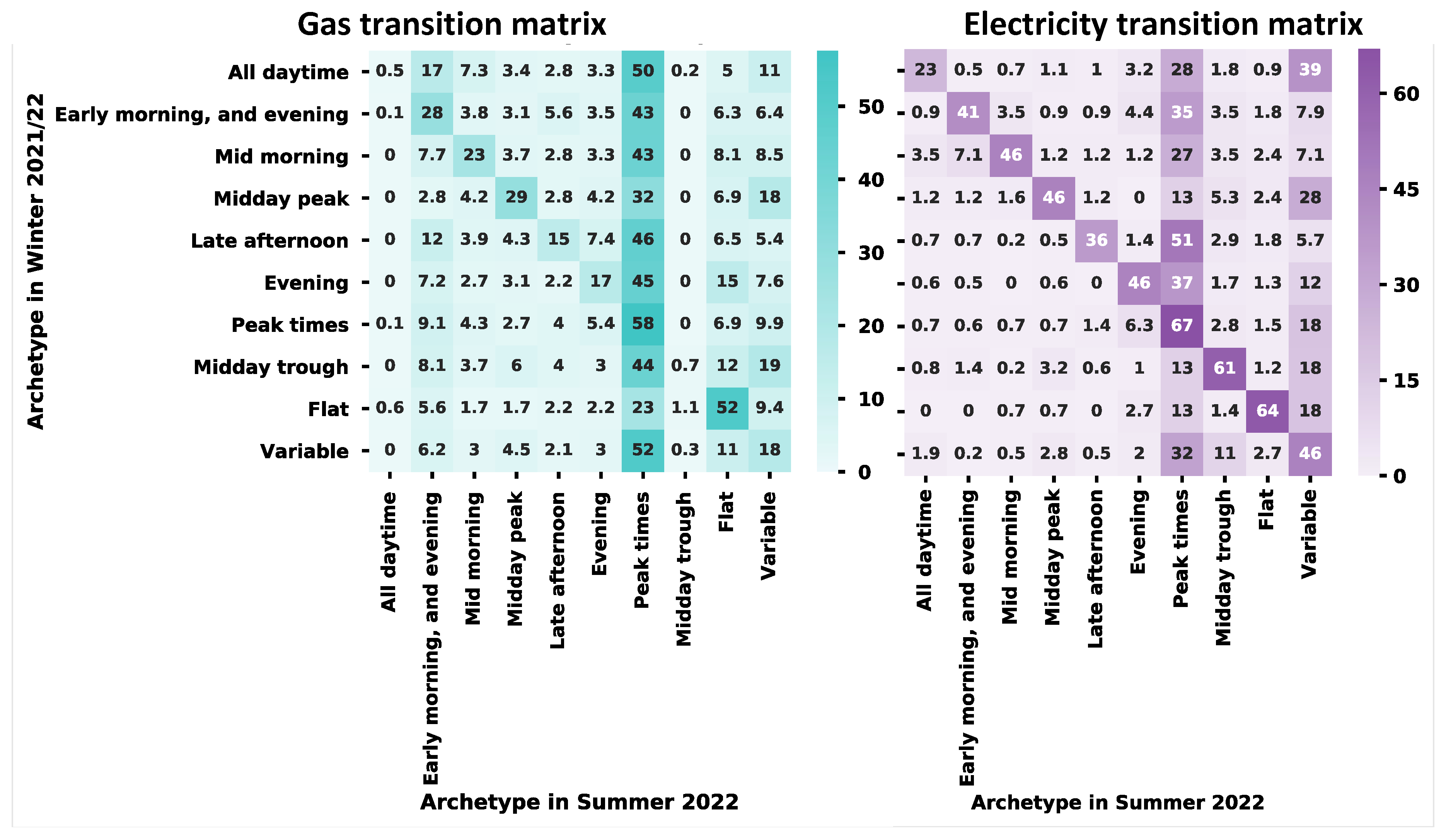
We next investigated how households’ demand archetypes transition between the winter weekday period and the summer weekday period, with results presented in the transition matrices in Error! Reference source not found.. In the case of gas profiles, the single most common transition from winter weekdays to summer weekdays is to the “Peak times” archetype, indicative of demand being highest during the morning or evening peak periods, but with variation from day to day. The second most common transition is generally to remain in the same archetype. There are a couple of notable exceptions – very few homes that fit the “All daytime” archetype on winter weekdays remain in it on summer weekdays. This is likely because it indicates the heating being on all through the daytime, a situation that is very unlikely to occur in summer. Homes in the “Flat” archetype on winter weekdays are most likely to remain in it on summer weekdays too – these could be homes that are unoccupied for extended periods, or that have a gas supply but make very little use of it during these periods.
For electricity, the pattern is similar to a degree, in that many homes transition to the “Peak times” archetype on summer weekdays; however, it is more common in most cases for a home to remain in the same archetype that it was in during the winter weekday period. The “Variable” archetype is also more common on summer weekdays than it is for gas. These results could be due to household electricity demand being, in most cases, less dominated by heating use than is the case for gas, so exhibiting less seasonal variation.
Overall, the results are consistent with what would be expected given that gas is the primary heating fuel in most households. They highlight the importance of not treating homes as static entities that can have a single demand archetype meaningfully ascribed to each of them throughout the year.
Figure 4.
Transition matrix, indicating the percentage probability of a home transitioning from a given energy demand archetype to any of the others between winter weekdays 2021-2022 and summer weekdays 2022. Darker shadings indicate higher percentages. Presented separately for gas and electricity (see main text for full details).
5.2. Technology and Occupant Factors that Explain a Household’s Demand Archetype on Winter Weekdays (2021–2022)
The second research question relates to identifying technology and occupant factors that explain a household’s dominant energy demand archetype over the winter weekday period, a time of year when total daily demand is at its highest, largely due to space heating requirements. The extent to which certain household characteristics explain archetype membership was investigated using binomial logistic regression models regressed onto the households’ demand archetypes, as described in the methodology (Section 4.2). The analyses focused on the winter weekday archetypes for 2021-2022.
Table 4 presents all the statistically significant (at above the 95% confidence interval) odds ratio2 results, arranged by demand archetype, first for electricity and then for gas. The full set of regression results is available in the Appendix (Section 9.2). While the regressions focused on which variables correlated with each archetype (the outcome variable), we are most interested in the importance of the different variables for explaining archetypes in general. Therefore, in this section we report on the results by explanatory variable rather than by archetype.
For net electricity demand, the most influential variable on any archetype is the presence of microgeneration (this generally corresponds with the ‘Midday trough’ electricity archetype, as microgeneration is in nearly all cases solar photovoltaics, and so produces electricity during the daytime resulting in a pronounced trough in net demand during the middle of the day, particularly on sunny days). Households with microgeneration are 44 times more likely to exhibit this electricity demand archetype than those without. A household with microgeneration is also 1.7 times more likely to exhibit the ‘Variable’ electricity demand archetype, while having lower odds of fitting the ‘Late afternoon’, ‘Peak times’, ‘Evening’ or ‘All daytime’ archetypes (around 3-5 times less likely).
Electric vehicle (EV) ownership increases the odds of a home fitting the ‘Variable’ electricity demand archetype, which could be the result of having inconsistent charging patterns from day to day. It reduces the odds of a household having a ‘Late afternoon’ electricity archetype (3.8 times less likely) or ‘Peak electricity’ archetype (1.5 times less likely), implying that charging is less likely to occur at these times, possibly due to electric vehicle-tailored tariffs that encourage off-peak charging. A surprising result is the association between EV ownership and increased odds of the ‘All daytime’ gas archetype. One possible explanation could be that homes with EVs may be more affluent on average and hence better able to afford heating throughout the whole day. Indeed, households with high financial wellbeing were around 1.5 times more likely to have an ‘All daytime’ archetype (for both electricity and gas), and around 1.9 times more likely to have an ‘Early morning, and evening’ gas archetype; a profile we would typically associate with everyone being out of the house during the day at work/school. In households with two adults this could imply a double income. Households with low financial wellbeing were more likely to have a ‘Variable’ (1.5 times) or ‘Peak’ (1.4 times) gas archetype; this would be consistent with these households limiting heating use to whenever they felt most need for it, although more investigation would be required to confirm if this is the true reason.
Family status (the combination of any/no working adults and any/no children)3 correlated statistically significantly with many of the electricity archetypes and some of the gas archetypes. While working from home has become more prevalent since the COVID-19 pandemic, clearly working patterns still affect occupancy and energy use. The reference category (no children, no one working) was less likely to be in the ‘Peak times’ archetypes for both electricity and gas than any other family status, which implies that non-working people are more likely to be using energy throughout the day, as we might expect (as they are more likely to be at home).
As expected, heating fuel is significantly related to some electricity archetypes. The ‘Midday trough’ archetype is 13 times more likely for homes with electric heating than gas heating. This could be related to the use of storage heaters, which are designed to draw electricity overnight and so lead to the home’s normalised daytime use of electricity being comparatively low. It could also be that the presence of electric heating may be correlated with microgeneration, since having both likely maximises the potential self-consumption of locally generated electricity. Both the ‘Late afternoon’ and ‘Peak times’ electricity archetypes are less likely for homes with electric heating rather than gas heating, again suggesting that these homes may take advantage of variable tariffs which encourage use of heating outside peak times. Homes with electric heating are also less likely to exhibit the ‘Variable’ electricity archetype than homes with gas heating, likely because heating constitutes a large load which is used in a regular manner, so leading to greater day-to-day consistency in the load profile.
Discussion
This paper investigated household electricity and gas demand archetypes, including the degree to which the archetype a household exhibits varies between winter weekdays and summer weekdays, and the extent to which a household’s typical winter weekday demand archetype is explained by their technology and occupant characteristics. The analyses focused on households in Great Britain between November 2021 and August 2022, and used the SERL Observatory dataset of smart meter and linked contextual data from 13,000 consented households (of which 13,208 had available electricity meter data, and 10,114 had gas data), as well as the results of a cluster analysis of the demand profiles from that dataset that we previously published. For the current study, 10,990 (for electricity) and 7,940 (for gas) of these homes had sufficient data to calculate household demand archetypes for both periods; 9,844 (for electricity) and 7,251 (for gas) had all the required data to investigate correlations between household characteristics and their demand archetypes in the winter weekday period,
The paper focused on two research questions, and the results pertaining to each of these are discussed below.
- What is the prevalence of each household demand archetype on winter weekdays and summer weekdays, and what transitions between demand archetypes are most common for households to make between these two periods?
Previous research which has developed household demand archetypes has often tried to control for predictable, rhythmic changes in factors that drive patterns of demand by developing different archetypes for homes for different periods of time (also termed ‘loading conditions’ and ‘contexts’ in some works). We followed this approach, defining separate periods based on season and weekdays vs. weekends, following previous literature, to control by proxy for external weather variations and weekly societal rhythms of work and schooling (and hence occupancy). Our work focused on two such periods: winter weekdays and summer weekdays (for 2021-2022, and 2022, respectively). The results showed that during these specific periods, approximately 90% of households had a dominant gas demand archetype (i.e. one that their demand profile fitted for more than 50% of the days in the period), although the single most common one, ‘Peak times’ still indicated substantial between-day variation in the extent to which peak demand occurred in the morning, evening, or both. For electricity, about 75% had a dominant demand archetype, although ‘Peak times’ accounted for over half of that 75%. Seasonal changes in the prevalence of these archetypes across the sample were particularly prominent for gas demand, as might be expected given its dominant role in heating in the UK. In particular, 15.4% of households fitted the ‘All daytime’ archetype in the winter weekday period, but this fell to just 0.2% in the summer weekday period. Electricity demand exhibited more variability than gas, with 23.2% of homes having no dominant archetype in either period. The prevalence across the sample of the different electricity demand archetypes changed little between the two periods, perhaps as most electricity uses are less shaped by weather. The exceptions were the ‘All daytime’ archetype, which was more common on winter weekdays than summer weekdays (8.7% vs 3.1% of households), and the ‘Midday trough’ archetype (5.0% of households in winter weekdays, 7.5% on summer weekdays). These results are consistent with a small proportion of homes using electricity for heating, and homes with solar PV having more electricity generated by their solar panels in summer, respectively. These results are consistent with previous literature in indicating that this is a valid approach to controlling for the large effects of external factors on household demand profiles, and that it is not empirically useful to attempt to identify a single demand archetype for a household across all periods (e.g. for an entire year).
- 2.
- What (if any) technology and occupant factors explain a household’s demand archetype on winter weekdays?
Logistic regression results showed that heating fuel, solar PV, presence of electric vehicles, family status (presence of workers and/or children) and level of financial wellbeing all impacted the odds ratios of at least two and up to all six of the electricity archetypes we investigated for the winter weekdays period. EV ownership, family status and financial wellbeing also impacted between one and four of the five gas archetypes tested for that period. For electricity, microgeneration heavily increased the probability of homes being in the ‘Midday trough’ archetype, consistent with substantial electricity generation by the solar panels during the middle hours of the day, while the results suggest that owning electric vehicles, whose charging is a large and potentially flexible load, can mean households are less likely to have any clearly dominating demand profile. These findings could be valuable for network operators trying to model and anticipate how network requirements may change in future with increased adoption of EVs and microgeneration. The result that EVs are associated with households being more likely to fit the ‘All daytime’ archetype for their gas use may be because EV-owning households are typically more affluent and able to afford more heating through the day. For both fuels, the correlations between family status and different archetypes are indicative of homes being more likely to be unoccupied during the middle of the day for households where formal workers and/or children are present compared to those with neither present. Households reporting low financial wellbeing were less likely to fit the ‘All daytime’ archetype and more likely to fit the ‘Variable’ archetype for both fuels, which is consistent with those households attempting to or having to limit their consumption.
The results highlight how grid energy demand from households results from a complex sociotechnical interaction between technology and occupants. The analysis in this study, focused as it is on net grid demand, therefore investigates these sociotechnical factors’ relationships to metered delivered energy, not the underlying service demand (such as demand for heating or lighting). When interpreting the results, this difference is important. For example, the household’s winter weekday gas demand archetype may not strongly correspond to the level and timing of heating the occupants have requested, as it can be mediated by the heating technology, building characteristics, levels of solar gain and more in a complex way. There is some evidence that how heating controls are set up when commissioned or installed can determine demand profiles, some of which are pre-programmed into controllers as defaults. Also, even with the same control settings, the delivered gas profile will change with the weather and fabric efficiency. For example, on a day when the controller is set to demand heat all day, the heating system will not necessary turn on and consume gas during the middle of the day when it is warmer outside and there are more solar gains. In addition, in a well-insulated modern house, a very significant proportion of space heat can be provided by incidental gains from lights, appliances, occupants and solar gains.
Future work
Future work could aim to investigate some of the influence of the interacting sociotechnical effects discussed above in more detail, exploring how heat service demand translates into grid energy demand. In addition, future work could valuably investigate the extent to which (currently) less common technologies and factors lead to other, different, demand archetypes. Heat pumps and/or time-of-use tariffs, including EV-specific tariffs that encourage off-peak charging or heating specific tariffs such as Economy-7 or those targeting heat pumps, would all be of policy and energy system interest. Although homes with such technologies and tariffs are present in the SERL Observatory dataset, consistent with the wider housing stock, they do not constitute a large proportion of the sample, and so any distinct demand archetypes that they exhibit are unlikely to have been identified in this study. These are, however, homes which might be expected to have distinct demand archetypes, and are of increasing relevance to the energy system and policy. The influence of further home and household-related characteristics on a household’s exhibited demand archetype would also be worth investigating; in particular, the effect of building size and fabric characteristics, or Energy Performance Certificate ratings, would be of policy interest. We also identified in this paper that homes with lower financial wellbeing were more likely to have varying gas demand on winter weekdays; future work could attempt to investigate if this is due to their being more likely to limit their heating use for cost reasons, perhaps through surveying participants in the study.
Future work could also valuably focus on methodological aspects of the research. It would be valuable to compare the results of our approach to defining a household’s demand archetype, based on its modal daily archetype over the period in question, with the wide range of other methods in the literature. Much published research generates household demand archetypes using cluster analysis based on measures of the household’s demand at each time over the day averaged over the period, often with some measure of between-day variability. By contrast, we look at the modal daily demand archetype over the period, consistent with the underlying concept that households (and their heating systems and solar panels) tend to have a typical daily rhythm within specific periods that leaves traces in their energy profiles, and it is that typical pattern that we were interested in revealing. Noting the large number of homes that had highly variable demand patterns in the study, another possible avenue of future work would be to explore the impact of using differently defined periods of time in which to identify household demand archetypes, to explore the extent to which these could better control for external factors and lead to fewer homes that have no clear demand archetype. In particular, periods could be based on external temperature bands rather than season, to better control for external weather effects.
6. Conclusion
This paper has investigated the electricity and gas demand archetypes of households in GB over the winter weekdays of 2021-2022, and summer weekdays of 2022. Consistent with previous work in this area, we find that it is more valid to identify a household’s demand archetype within specific periods of time defined by seasons and weekdays vs weekend, rather than for entire years, to control for some of the otherwise substantial day-to-day variation over time. Methods to define a household’s demand archetype are in effect attempting to smooth out day-to-day fluctuations in their demand profiles and help focus on the household’s underlying ‘default’ pattern under a particular set of external conditions. This ‘default’ for the home, and which socio-technical factors affect it, provide policymakers and practitioners with more evidence of how socio-technical change and interventions might impact on the timings of peak demand in future. To that end, we introduced a method that focuses on the households’ modal, i.e. most common, daily demand archetype within each period, an approach we have not previously identified in the literature. This has an advantage of allowing direct comparability between demand archetypes that pertain to a home within a particular period and those that relate to individual days per home, so that variation and stability can be analysed and compared for different units of analysis. The SERL Observatory dataset used in this study also allowed us to investigate households’ electricity and gas demand profiles separately, and for periods after the COVID-19 pandemic, unlike other research identified.
On winter weekdays, households most commonly exhibit gas demand archetypes that point to substantial amounts of space heating, consistent with heating that coincides with morning and evening peak periods, or that is used throughout the daytime; the ‘All daytime’ archetype is far less common on summer weekdays. For electricity, archetypes are primarily ‘Peak times’ or ‘Variable’, with far less variation between winter weekday and summer weekday periods. Consistent with previous literature, and with expectations, a household’s demand archetype is affected by major technological factors (heating fuel used, presence of EVs and of microgeneration), and occupant characteristics (family status and financial wellbeing).
7. CRediT Authorship Contribution Statement
Martin Pullinger: Conceptualisation, Methodology, Software, Formal analysis, Writing – Original Draft, Writing - Review & Editing, Visualisation.
Ellen Zapata-Webborn: Methodology, Software, Formal analysis, Writing – Original Draft, Writing - Review & Editing
Jonathan Kilgour: Methodology, Software, Formal analysis, Writing - Review & Editing.
Minnie Ashdown: Writing - Review & Editing.
Simon Elam: Funding acquisition, project administration.
Jessica Few: Writing - Review & Editing.
Nigel Goddard: Funding acquisition.
Clare Hanmer: Writing - Review & Editing.
Frances Hollick: Writing - Review & Editing.
Tadj Oreszczyn: Funding acquisition, Writing - Review & Editing.
Lin Zheng: Writing - Review & Editing.
8. Acknowledgments
This article is based on research funded by UKRI, the Engineering and Physical Sciences Research Council projects Smart Energy Research Lab, grant number EP/P032761/1 and Energy Demand Observatory and Laboratory, grant number EP/X00967X/1. Particular thanks go to the SERL team within UCL: James O'Toole for project administration and Cristian Dinu for software, data curation and dataset development; and at the UK Data Archive: Darren Bell, Deirdre Lungley, Martin Randall and Jacob Joy, also for software, data curation and dataset development. Support from the SERL Advisory Board, Data Governance Board and Research Programme Board played a critical role in the establishment and ethical operation of SERL. We would also like to thank the 13,000+ SERL Observatory households who have consented access to their smart meter data, without whom it would not have been possible to undertake this research.
9. Appendix
9.1. Data Availability
The SERL Observatory dataset used in this research continues to be collected and periodically released for use by UK accredited researchers on approved projects [14,18].
Data: Elam, S., Webborn, E., Few, J., McKenna, E., Pullinger, M., Oreszczyn, T., Anderson, B., Ministry of Housing, Communities and Local Government, European Centre for Medium-Range Weather Forecasts, Royal Mail Group Limited. (2023). Smart Energy Research Lab Observatory Data, 2019-2022: Secure Access. [data collection]. 5th Edition. UK Data Service. SN: 8666, DOI: http://doi.org/10.5255/UKDA-SN-8666-6
Data descriptor: Webborn E, Few J, McKenna E, Elam S, Pullinger M, Anderson B, et al. The SERL Observatory Dataset: Longitudinal Smart Meter Electricity and Gas Data, Survey, EPC and Climate Data for Over 13,000 GB Households. Energies (Basel) 2021;14. https://doi.org/10.3390/en14216934.
9.2. Logistic Regression Results
Full logistic regression results are presented in Table 5 below. See section 5.2 for details.
Glossary
•Daily demand profile: the pattern of electricity or gas demand from a single household over the course of one day.
•Household demand profile: the typical pattern of electricity or gas demand from a single household over a specified period of many days. ‘Typical’ could be the mean or median demand for each period of the day, but varies by study.
•Daily demand archetype: across a sample of homes, based on data for a period of many days, common daily demand profiles can be identified using cluster analysis, which we refer to as daily demand archetypes. Each ‘case’ used as an input into the cluster analysis is one day of data from one home, typically considering one fuel (electricity or gas) in isolation, or treating each as separate cases.
•Household demand archetypes: common household demand profiles identified in the same data for a specified period of time. Unlike daily demand archetypes, which can vary both between homes on a given day, and over time for a given home, household demand archetypes represent a home’s typical demand profile for a period of many days (e.g. for a heating season), and so are fixed for a given home for specified periods of time.
•Time period, or simply “period”: In the context of this paper, this refers to distinct periods of time for which a household’s demand archetype is separately identified. In the literature, such periods are also referred to as “loading conditions” and “contexts”, and may include repeating time slices over a period of time, for example, weekdays over winter; weekends over summer. See the literature review for more details of the underlying rationale.
•Winter weekdays: In the context of this paper, this refers specifically to Monday to Friday for the 13 full weeks from 30 November 2021 to 28 February 2022 inclusive. The term is italicised throughout to indicate that it is referring to this specific period.
•Summer weekdays: In the context of this paper, this refers specifically to Mondays to Fridays for the 13 weeks from 2 June to 31 August 2022 inclusive. The term is italicised throughout to indicate that it is referring to this specific period.
References
- Rajabi A, Eskandari M, Jabbari M, Li L, Zhang J. A comparative study of clustering techniques for electrical load pattern segmentation. Renewable and Sustainable Energy Reviews 2020;120. [CrossRef]
- Trotta G. An empirical analysis of domestic electricity load profiles: Who consumes how much and when? Appl Energy 2020;275:115399. [CrossRef]
- Fernandes MP, Viegas JL, Vieira SM, Sousa JM. Analysis of residential natural gas consumers using fuzzy c-means clustering. 2016 IEEE International Conference on Fuzzy Systems (FUZZ-IEEE), 2016, p. 1484–91. [CrossRef]
- Zapata-Webborn E, McKenna E, Pullinger M, Cheshire C, Masters H, Whittaker A, et al. The impact of COVID-19 on household energy consumption in England and Wales from April 2020 to March 2022. Energy Build 2023;297:113428. [CrossRef]
- Hanmer C, McKenna E, Zapata-Webborn E, Few J, Pullinger M. The impact of the ‘cost of living crisis’ in Britain: energy saving actions by fuel-poor households in winter 2022/23. Proceedings of eceee 2024 Summer Study on Energy Efficiency, European Council for an Energy Efficient Economy; 2024.
- Yilmaz S, Chambers J, Patel MK. Comparison of Clustering Approaches for Domestic Electricity Load Profile Characterisation-{{Implications}} for Demand Side Management. Energy 2019;180:665–77. [CrossRef]
- Li H, Wang Z, Hong T, Parker A, Neukomm M. Characterizing patterns and variability of building electric load profiles in time and frequency domains. Appl Energy 2021;291:116721. [CrossRef]
- Räsänen T, Voukantsis D, Niska H, Karatzas K, Kolehmainen M. Data-based method for creating electricity use load profiles using large amount of customer-specific hourly measured electricity use data. Appl Energy 2010;87:3538–45. [CrossRef]
- Trotta G. An empirical analysis of domestic electricity load profiles: Who consumes how much and when? Appl Energy 2020;275:115399. [CrossRef]
- Fernandes M, Viegas J, Vieira S, Sousa J. Segmentation of Residential Gas Consumers Using Clustering Analysis. Energies (Basel) 2017;10:2047. [CrossRef]
- Fernandes MP, Viegas JL, Vieira SM, Sousa JM. Analysis of residential natural gas consumers using fuzzy c-means clustering. 2016 IEEE International Conference on Fuzzy Systems (FUZZ-IEEE), 2016, p. 1484–91. [CrossRef]
- Czétány L, Vámos V, Horváth M, Szalay Z, Mota-Babiloni A, Deme-Bélafi Z, et al. Development of electricity consumption profiles of residential buildings based on smart meter data clustering. Energy Build 2021;252:111376. [CrossRef]
- Lee E, Kim J, Jang D. Load Profile Segmentation for Effective Residential Demand Response Program: Method and Evidence from Korean Pilot Study. Energies (Basel) 2020;13:1348. [CrossRef]
- Han F, Pu T, Li M, Taylor G. Short-term forecasting of individual residential load based on deep learning and K-means clustering. CSEE Journal of Power and Energy Systems 2021;7:261–9. [CrossRef]
- Alonso AM, Martín E, Mateo A, Nogales FJ, Ruiz C, Veiga A. Clustering Electricity Consumers: Challenges and Applications for Operating Smart Grids. IEEE Power and Energy Magazine 2022;20:54–63. [CrossRef]
- Pullinger M, Zapata-Webborn E, Kilgour J, Elam S, Few J, Goddard N, et al. Capturing variation in daily energy demand profiles over time with cluster analysis in British homes (September 2019 – August 2022). Appl Energy 2024;360:122683. [CrossRef]
- Zapata-Webborn E, McKenna E, Pullinger M, Cheshire C, Masters H, Whittaker A, et al. The impact of COVID-19 on household energy consumption in England and Wales from April 2020 – March 2022. Forthcoming 2023.
- Pinto S, Gorman R. Understanding Great Britain’s energy consumption patterns through smart meter data 2025. https://www.nesta.org.uk/report/understanding-gb-energy-consumption-patterns/ (accessed August 25, 2025).
- Smart Energy Research Lab. Welcome to the Smart Energy Research Lab n.d.
- Webborn E, Elam S, McKenna E, Oreszczyn T. Utilising smart meter data for research and innovation in the UK. Proceedings of ECEEE 2019 Summer Study on energy efficiency. ECEEE: Belambra Presqu’île de Giens, France, 2019, p. 1387–96.
- Webborn E, Few J, McKenna E, Elam S, Pullinger M, Anderson B, et al. The SERL Observatory Dataset: Longitudinal Smart Meter Electricity and Gas Data, Survey, EPC and Climate Data for Over 13,000 GB Households. Energies (Basel) 2021;14. [CrossRef]
- Elam S, Webborn E, Few J, McKenna E, Pullinger M, Oreszczyn T, et al. Smart Energy Research Lab Observatory Data, 2019-2022: Secure Access. 6th Edition. UK Data Service 2023. [CrossRef]
- Satre-Meloy A, Diakonova M, Grünewald P. Cluster Analysis and Prediction of Residential Peak Demand Profiles Using Occupant Activity Data. Appl Energy 2020;260:114246. [CrossRef]
- Czétány L, Vámos V, Horváth M, Szalay Z, Mota-Babiloni A, Deme-Bélafi Z, et al. Development of electricity consumption profiles of residential buildings based on smart meter data clustering. Energy Build 2021;252:111376. [CrossRef]
- Pinto S, Gorman R. Technical appendix: Using smart meters to identify energy use profiles 2025. https://media.nesta.org.uk/documents/Energy_profiles__technical_appendix_2nd_phase_results_.pdf (accessed August 25, 2025).
- Fernandes M, Viegas J, Vieira S, Sousa J. Segmentation of Residential Gas Consumers Using Clustering Analysis. Energies (Basel) 2017;10:2047. [CrossRef]
- Fernandes MP, Viegas JL, Vieira SM, Sousa JMC. Seasonal Clustering of Residential Natural Gas Consumers. In: Carvalho J, Lesot MJ, Kaymak U, Vieira S, Bouchon-Meunier B, Yager R, editors. Information Processing and Management of Uncertainty in Knowledge-Based Systems. IPMU 2016. Communications in Computer and Information Science, vol 610., Cham: Springer; 2016, p. 723–34. [CrossRef]
- Walker G. The dynamics of energy demand: Change, rhythm and synchronicity. Energy Res Soc Sci 2014;1:49–55. [CrossRef]
- Few J, Pullinger M, McKenna E, Elam S, Ashdown M, Hanmer C, et al. Smart Energy Research Lab: Energy use in GB domestic buildings 2022 and 2023. Smart Energy Research Lab (SERL) Statistical Reports Volume 2. London, UK: 2024.
- Pinto S, Gorman R. Energy use profiles explorer 2025. https://energy-use-profiles-explorer.dap-tools.uk/ (accessed August 25, 2025).
- ECMWF. ERA5: data documentation. ECMWF 2021.
- Few J, Pullinger M, McKenna E, Elam S, Webborn E, Oreszczyn T. Smart Energy Research Lab: Energy use in GB domestic buildings 2021. Smart Energy Research Lab (SERL) Statistical Reports Volume 1. London, UK: 2022.
- UK Government. Prime Minister confirms move to Plan B in England - GOV.UK 2021. https://www.gov.uk/government/news/prime-minister-confirms-move-to-plan-b-in-england (accessed August 29, 2025).
- UK Government. England returns to Plan A as regulations on face coverings and COVID Passes change today - GOV.UK 2022. https://www.gov.uk/government/news/england-returns-to-plan-a-as-regulations-on-face-coverings-and-covid-passes-change-today (accessed August 29, 2025).
- Zapata-Webborn E, McKenna E, Pullinger M, Cheshire C, Masters H, Whittaker A, et al. The impact of COVID-19 on household energy consumption in England and Wales from April 2020 – March 2022. Forthcoming 2023.
- Van Rossum G, Drake FL. Python 3 Reference Manual. Scotts Valley, CA: CreateSpace; 2009.
- McKinney W. Data Structures for Statistical Computing in Python. In: van der Walt S, Millman J, editors. Proceedings of the 9th Python in Science Conference, 2010, p. 56–61. [CrossRef]
- Harris CR, Millman KJ, van der Walt SJ, Gommers R, Virtanen P, Cournapeau D, et al. Array programming with NumPy. Nature 2020;585:357–62. [CrossRef]
- Pedregosa F, Varoquaux G, Gramfort A, Michel V, Thirion B, Grisel O, et al. Scikit-learn: Machine Learning in Python. Journal of Machine Learning Research 2011;12:2825–30.
- Virtanen P, Gommers R, Oliphant TE, Haberland M, Reddy T, Cournapeau D, et al. SciPi 1.0: Fundamental Algorithms for Scientific Computing in Python. Nat Methods 2020;17:161–272. [CrossRef]
- Kluyver T, Ragan-Kelley B, Perez F, Granger B, Bussonnier MA, Frederic J, et al. Jupyter Notebooks - a publishing format for reproducible computational workflows. In: Schmidt B, Loizides F, editors. Positioning and Power in Academic Publishing: Players, Agents and Agendas, 2016, p. 87–90.
- Hunter JD. Matplotlib: A 2D graphics environment. Comput Sci Eng 2007;9:90–5. [CrossRef]
- Waskom ML. seaborn: statistical data visualization. J Open Source Softw 2021;6:3021. [CrossRef]
- R Core Team. R: A language and environment for statistical computing 2023.
- Kuhn M. Classification and Regression Training 2022:https://CRAN.R-project.org/package=caret.
- Dowle M, Srinivasan A. data.table: Extension of `data.frame` 2022.
- Friedman J, Hastie T, Tibshirani R. Regularization Paths for Generalized Linear Models via Coordinate Descent. J Stat Softw 2010;33:1–22.
Figure 1.
Mean energy use over the day for each daily demand archetype, for each of: the two years September 2020 - 31 August 2022; Winter 2021-2022 (30 November 2021 - 28 February 2022); Summer 2022 (2 June - 31 August 2022). Electricity and gas shown separately. Note different y-axis scales for the two fuels. Reproduced from Pullinger et al 2024 [16].
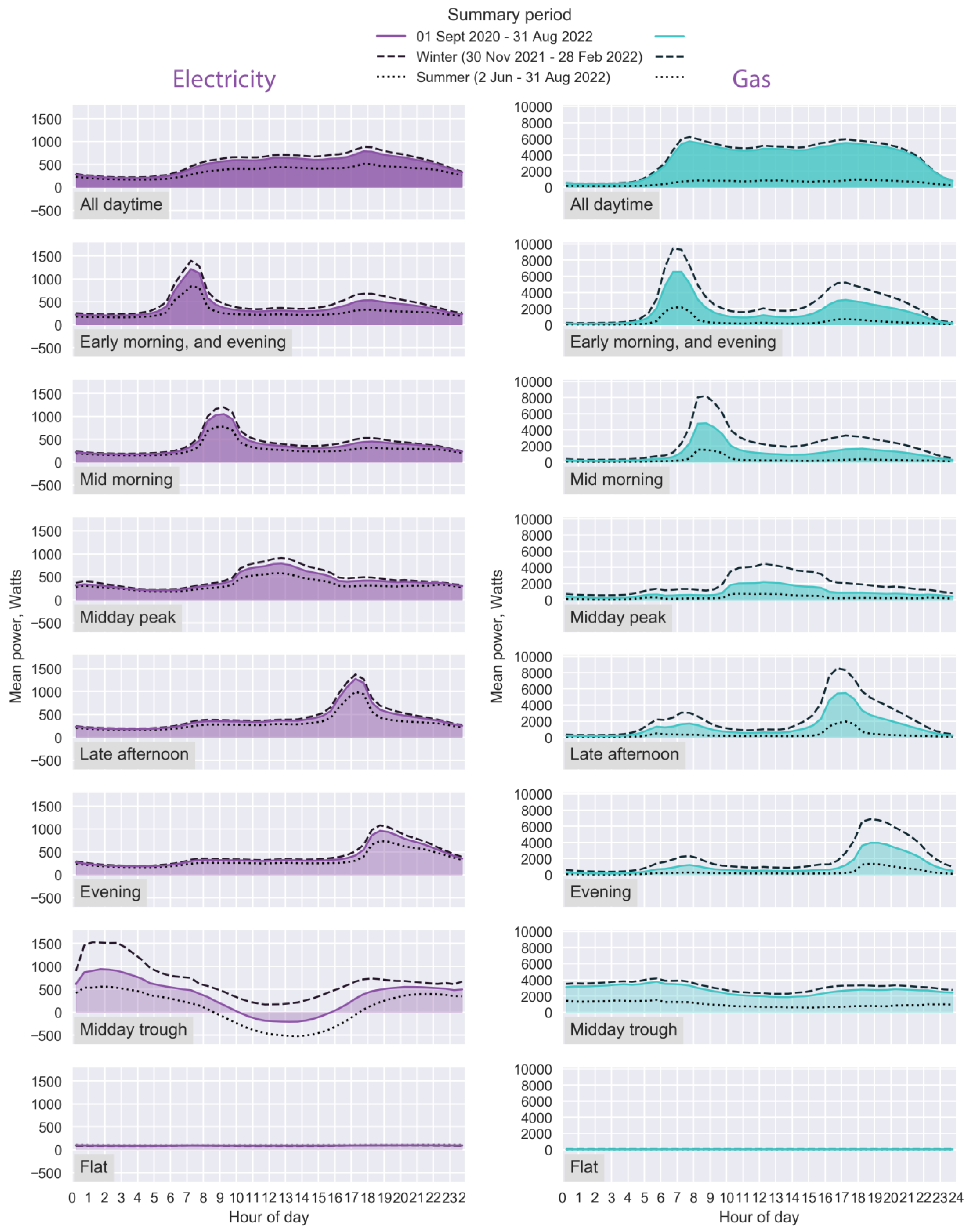
Figure 2.
Violin plot showing the percentage of days that homes change daily demand archetype in the two years ending August 2022. Presented separately for gas and electricity. Dotted line indicates 2/7th (28.6%), the value that would be expected for a notional household that changed profile twice per week on average, such as one consistently exhibiting a different weekday and weekend profile. N = 12,824 (electricity); 9,654 (gas).
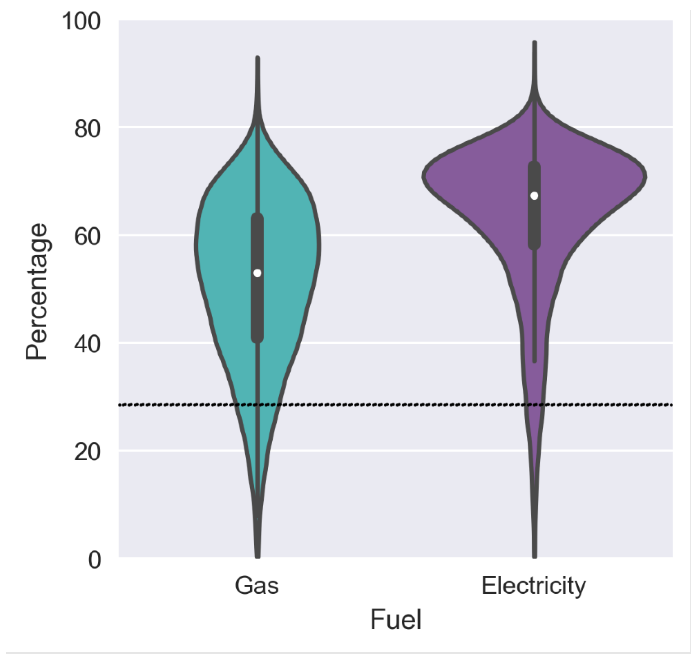
Figure 3.
Workflow to create household demand archetypes from daily demand profiles. Steps 1 to 3 were undertaken in previous work – see Pullinger et al 2024 [16] for details.*There are a few exceptions to this process due to missing data or lack of a dominant daily demand archetype – see Error! Reference source not found. for details.
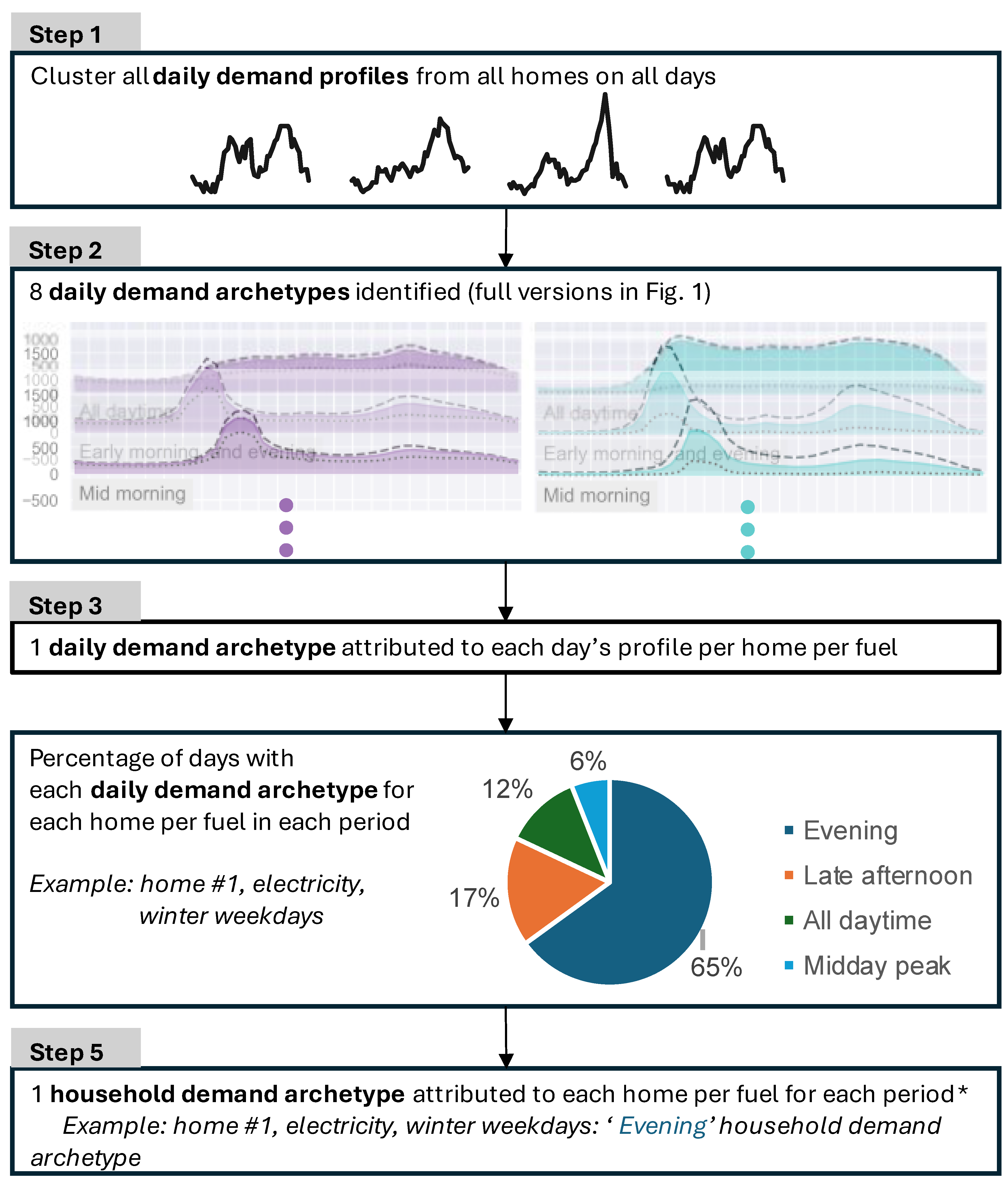

Table 1.
Definitions of each household demand archetype defined in this paper.
| Household demand archetype | Definition |
|---|---|
| ‘Missing’ | If >50% of days for the home and fuel have no allocated daily demand archetype due to missing data, then the household demand archetype is labelled as “Missing” |
|
‘All daytime’ ‘Early morning, and evening’ ‘Mid morning’ ‘Midday peak’ ‘Late afternoon’ ‘Evening’ ‘Midday trough’ ‘Flat’ |
For the given period, if >50% of non-missing days for the home and fuel exhibit the same daily demand archetype, then that is considered to be the home’s household demand archetype for that period. For example, if more than half of the days fitted the ‘All daytime’ archetype for gas use for home A for the given period, then its household gas demand archetype would also be ‘All daytime’ for that period. Figure 1 shows the typical demand profile of each of these archetypes. |
| ‘Mostly peak use’ | Of those still not labelled, if over 50% of the non-missing days belonged to a daily demand archetype for which most demand coincides with national peak times (i.e. ‘Early morning, and evening’, ‘Mid morning’, ‘Late afternoon’ and ‘Evening’), the household demand archetype was labelled ‘Mostly peak use’. |
| ‘Variable’ | Any remaining household demand archetypes were labelled as ‘Variable’ – there was no dominant daily demand archetype in the period for that fuel for that home. |
Table 2.
Winter weekday household demand archetypes per fuel, indicating number of cases (households) in each and whether a logistic regression model was fitted to them. (See Figure 1 and Table 1 for more information about these demand archetypes).
| Archetype | Electricity | Gas | ||
|---|---|---|---|---|
| N homes | Logistic regression? | N homes | Logistic regression? | |
| All daytime | 874 | Yes | 1133 | Yes |
| Early morning, and evening | 178 | No | 1760 | Yes |
| Mid morning | 105 | No | 256 | No |
| Midday peak | 241 | No | 71 | No |
| Late afternoon | 532 | Yes | 522 | Yes |
| Evening | 1091 | Yes | 251 | No |
| Midday trough | 492 | Yes | 263 | No |
| Flat | 154 | No | 173 | No |
| Peak times | 3865 | Yes | 2002 | Yes |
| Variable | 2312 | Yes | 819 | Yes |
Table 3.
Prevalence of household demand archetypes for gas and electricity for winter weekdays (2021-2022) and summer weekdays (2022). Darker shadings correspond to higher percentages.
Table 3.
Prevalence of household demand archetypes for gas and electricity for winter weekdays (2021-2022) and summer weekdays (2022). Darker shadings correspond to higher percentages.
| Fuel: | Gas | Electricity | ||
|---|---|---|---|---|
|
Period: Household demand archetype |
Winter weekdays (%) |
Summer weekdays (%) |
Winter weekdays (%) |
Summer weekdays (%) |
| All daytime | 15.4 | 0.2 | 8.7 | 3.1 |
| Early morning, and evening | 23.2 | 16.4 | 1.7 | 1.4 |
| Mid morning | 3.3 | 5.6 | 1 | 1.1 |
| Midday peak | 1 | 3.4 | 2.4 | 2.6 |
| Late afternoon | 6.9 | 4.9 | 5.3 | 3.3 |
| Evening | 3.4 | 5.5 | 10.7 | 10.2 |
| Midday trough | 3.8 | 0.1 | 5 | 7.5 |
| Flat | 2.4 | 8.2 | 1.6 | 2.5 |
| Peak times | 26.8 | 43.9 | 39.1 | 42.7 |
| Variable | 11.6 | 8.8 | 23.2 | 23.2 |
| Missing | 2.2 | 3.1 | 1.2 | 2.5 |
Counts: Gas, winter weekdays: 8815; gas, summer weekdays: 8388; electricity, winter weekdays: 11870; electricity, summer weekdays: 11441.
Table 4.
Logistic regression results showing the odds ratios of households with different characteristics exhibiting each archetype on winter weekdays 2021-2022. Electricity and gas results presented separately. Blues indicate lower odds ratios (below 1) – darker is lower; greens indicate higher odds ratios (above 1) – darker is higher. The table only presents results that are statistically significant to at least the 95% confidence interval, sorted by fuel, archetype, explanatory variable and then odds ratio. For the full set of results, see the Appendix, section 9.2.
| Archetype | Variable | Value | Reference category | Odds ratio | p value |
|---|---|---|---|---|---|
| Electricity results | |||||
| All daytime | Family status | Workers, children | No workers, no children | 0.772 | 0.015 |
| Family status | Workers, no children | No workers, no children | 0.626 | 0.000 | |
| Financial wellbeing | Low | High | 0.675 | 0.000 | |
| Presence of microgeneration | Microgen present | No microgeneration | 0.202 | 0.000 | |
| Intercept | Intercept | - | 0.138 | 0.000 | |
| Late afternoon | Family status | Workers, children | No workers, no children | 0.683 | 0.004 |
| Family status | Workers, no children | No workers, no children | 0.527 | 0.000 | |
| Heating fuel | Oil | Gas | 1.611 | 0.010 | |
| Heating fuel | Electric | Gas | 0.490 | 0.013 | |
| Presence of Electric Vehicles | 1+ EVs present | No EVs | 0.260 | 0.003 | |
| Presence of microgeneration | Microgen present | No microgeneration | 0.327 | 0.000 | |
| Intercept | Intercept | - | 0.085 | 0.000 | |
| Evening | Family status | Workers, no children | No workers, no children | 1.909 | 0.000 |
| Family status | Workers, children | No workers, no children | 1.352 | 0.003 | |
| Presence of microgeneration | Microgen present | No microgeneration | 0.200 | 0.000 | |
| Intercept | Intercept | - | 0.096 | 0.000 | |
| Midday trough | Family status | Workers, no children | No workers, no children | 0.744 | 0.012 |
| Family status | Workers, children | No workers, no children | 0.644 | 0.016 | |
| Heating fuel | Electric | Gas | 13.062 | 0.000 | |
| Heating fuel | None | Gas | 9.075 | 0.000 | |
| Presence of microgeneration | Microgen present | No microgeneration | 43.964 | 0.000 | |
| Intercept | Intercept | - | 0.017 | 0.000 | |
| Peak times | Family status | Workers, children | No workers, no children | 1.776 | 0.000 |
| Family status | No workers, children | No workers, no children | 1.544 | 0.010 | |
| Family status | Workers, no children | No workers, no children | 1.370 | 0.000 | |
| Heating fuel | Electric | Gas | 0.467 | 0.000 | |
| Heating fuel | None | Gas | 0.456 | 0.000 | |
| Presence of Electric Vehicles | 1+ EVs present | No EVs | 0.669 | 0.001 | |
| Presence of microgeneration | Microgen present | No microgeneration | 0.230 | 0.000 | |
| Intercept | Intercept | - | 0.586 | 0.000 | |
| Variable | Family status | Workers, no children | No workers, no children | 0.885 | 0.020 |
| Family status | Workers, children | No workers, no children | 0.732 | 0.000 | |
| Financial wellbeing | Low | High | 1.137 | 0.032 | |
| Heating fuel | District | Gas | 1.838 | 0.008 | |
| Presence of Electric Vehicles | 1+ EVs present | No EVs | 1.926 | 0.000 | |
| Presence of microgeneration | Microgen present | No microgeneration | 1.686 | 0.000 | |
| Heating fuel | Electric | Gas | 0.582 | 0.000 | |
| Intercept | Intercept | - | 0.312 | 0.000 | |
| Gas results | |||||
| All daytime | Family status | Workers, no children | No workers, no children | 0.520 | 0.000 |
| Family status | No workers, children | No workers, no children | 0.445 | 0.012 | |
| Family status | Workers, children | No workers, no children | 0.343 | 0.000 | |
| Financial wellbeing | Low | High | 0.699 | 0.000 | |
| Presence of Electric Vehicles | 1+ EVs present | No EVs | 1.608 | 0.002 | |
| Intercept | Intercept | - | 0.294 | 0.000 | |
| Early morning, and evening | Family status | Workers, children | No workers, no children | 1.751 | 0.000 |
| Financial wellbeing | Low | High | 0.542 | 0.000 | |
| Intercept | Intercept | - | 0.313 | 0.000 | |
| Late afternoon | Family status | Workers, no children | No workers, no children | 1.290 | 0.011 |
| Intercept | Intercept | - | 0.071 | 0.000 | |
| Peak times | Family status | Workers, children | No workers, no children | 1.442 | 0.000 |
| Family status | Workers, no children | No workers, no children | 1.426 | 0.000 | |
| Financial wellbeing | Low | High | 1.352 | 0.000 | |
| Intercept | Intercept | - | 0.291 | 0.000 | |
| Variable | Financial wellbeing | Low | High | 1.499 | 0.000 |
| Intercept | Intercept | - | 0.109 | 0.000 | |
Table 5.
Full logistic regression results for homes’ archetypes during winter weekdays (2021-2022). Electricity and gas results presented separately. In the Odds ratio column, blues indicate lower odds ratios (below 1) – darker is lower; greens indicate higher odds ratios (above 1) – darker is higher. In the p-value column, green indicates results that are statistically significant at the 5 percent level.
| Archetype | Variable | Value | Reference category | Odds ratio | p value | Esti-mate | Standard error | Stat-istic |
|---|---|---|---|---|---|---|---|---|
| Electricity | ||||||||
| All daytime | Family status | No workers, children | No workers, no children | 1.263 | 0.356 | 0.23 | 0.25 | 0.92 |
| All daytime | Family status | Workers, children | No workers, no children | 0.772 | 0.015 | -0.26 | 0.11 | -2.44 |
| All daytime | Family status | Workers, no children | No workers, no children | 0.626 | 0.000 | -0.47 | 0.08 | -5.91 |
| All daytime | Financial wellbeing | Low | High | 0.675 | 0.000 | -0.39 | 0.10 | -4.01 |
| All daytime | Heating fuel | None | Gas | 1.571 | 0.098 | 0.45 | 0.27 | 1.65 |
| All daytime | Heating fuel | Electric | Gas | 1.252 | 0.149 | 0.22 | 0.16 | 1.44 |
| All daytime | Heating fuel | Oil | Gas | 0.927 | 0.682 | -0.08 | 0.18 | -0.41 |
| All daytime | Heating fuel | District | Gas | 0.908 | 0.809 | -0.10 | 0.40 | -0.24 |
| All daytime | Heating fuel | Others | Gas | 0.859 | 0.683 | -0.15 | 0.37 | -0.41 |
| All daytime | Presence of Electric Vehicles | 1+ EVs present | No EVs | 0.628 | 0.053 | -0.47 | 0.24 | -1.94 |
| All daytime | Presence of microgeneration | Microgen present | No microgeneration | 0.202 | 0.000 | -1.60 | 0.27 | -5.85 |
| All daytime | Intercept | Intercept | - | 0.138 | 0.000 | -1.98 | 0.06 | -35.27 |
| Late afternoon | Family status | No workers, children | No workers, no children | 0.854 | 0.653 | -0.16 | 0.35 | -0.45 |
| Late afternoon | Family status | Workers, children | No workers, no children | 0.683 | 0.004 | -0.38 | 0.13 | -2.85 |
| Late afternoon | Family status | Workers, no children | No workers, no children | 0.527 | 0.000 | -0.64 | 0.10 | -6.33 |
| Late afternoon | Financial wellbeing | Low | High | 0.874 | 0.248 | -0.13 | 0.12 | -1.16 |
| Late afternoon | Heating fuel | Oil | Gas | 1.611 | 0.010 | 0.48 | 0.18 | 2.58 |
| Late afternoon | Heating fuel | Others | Gas | 1.031 | 0.942 | 0.03 | 0.43 | 0.07 |
| Late afternoon | Heating fuel | None | Gas | 1.018 | 0.963 | 0.02 | 0.39 | 0.05 |
| Late afternoon | Heating fuel | District | Gas | 0.607 | 0.399 | -0.50 | 0.59 | -0.84 |
| Late afternoon | Heating fuel | Electric | Gas | 0.490 | 0.013 | -0.71 | 0.29 | -2.49 |
| Late afternoon | Presence of Electric Vehicles | 1+ EVs present | No EVs | 0.260 | 0.003 | -1.35 | 0.45 | -2.97 |
| Late afternoon | Presence of microgeneration | Microgen present | No microgeneration | 0.327 | 0.000 | -1.12 | 0.28 | -3.92 |
| Late afternoon | Intercept | Intercept | - | 0.085 | 0.000 | -2.46 | 0.07 | -36.02 |
| Evening | Family status | Workers, no children | No workers, no children | 1.909 | 0.000 | 0.65 | 0.07 | 8.80 |
| Evening | Family status | Workers, children | No workers, no children | 1.352 | 0.003 | 0.30 | 0.10 | 2.96 |
| Evening | Family status | No workers, children | No workers, no children | 0.723 | 0.353 | -0.32 | 0.35 | -0.93 |
| Evening | Financial wellbeing | Low | High | 0.915 | 0.284 | -0.09 | 0.08 | -1.07 |
| Evening | Heating fuel | District | Gas | 1.256 | 0.471 | 0.23 | 0.32 | 0.72 |
| Evening | Heating fuel | Others | Gas | 1.164 | 0.614 | 0.15 | 0.30 | 0.50 |
| Evening | Heating fuel | Oil | Gas | 1.027 | 0.871 | 0.03 | 0.16 | 0.16 |
| Evening | Heating fuel | Electric | Gas | 0.798 | 0.176 | -0.23 | 0.17 | -1.35 |
| Evening | Heating fuel | None | Gas | 0.686 | 0.259 | -0.38 | 0.33 | -1.13 |
| Evening | Presence of Electric Vehicles | 1+ EVs present | No EVs | 0.708 | 0.092 | -0.35 | 0.21 | -1.69 |
| Evening | Presence of microgeneration | Microgen present | No microgeneration | 0.200 | 0.000 | -1.61 | 0.26 | -6.28 |
| Evening | Intercept | Intercept | - | 0.096 | 0.000 | -2.34 | 0.06 | -37.52 |
| Midday trough | Family status | Workers, no children | No workers, no children | 0.744 | 0.012 | -0.30 | 0.12 | -2.52 |
| Midday trough | Family status | Workers, children | No workers, no children | 0.644 | 0.016 | -0.44 | 0.18 | -2.40 |
| Midday trough | Family status | No workers, children | No workers, no children | 0.522 | 0.178 | -0.65 | 0.48 | -1.35 |
| Midday trough | Financial wellbeing | Low | High | 1.109 | 0.460 | 0.10 | 0.14 | 0.74 |
| Midday trough | Heating fuel | Electric | Gas | 13.062 | 0.000 | 2.57 | 0.15 | 16.68 |
| Midday trough | Heating fuel | None | Gas | 9.075 | 0.000 | 2.21 | 0.29 | 7.55 |
| Midday trough | Heating fuel | Oil | Gas | 1.290 | 0.293 | 0.25 | 0.24 | 1.05 |
| Midday trough | Heating fuel | Others | Gas | 0.850 | 0.780 | -0.16 | 0.58 | -0.28 |
| Midday trough | Heating fuel | District | Gas | 0.000 | 0.960 | -12.73 | 251.48 | -0.05 |
| Midday trough | Presence of Electric Vehicles | 1+ EVs present | No EVs | 1.494 | 0.065 | 0.40 | 0.22 | 1.85 |
| Midday trough | Presence of microgeneration | Microgen present | No microgeneration | 43.964 | 0.000 | 3.78 | 0.12 | 31.21 |
| Midday trough | Intercept | Intercept | - | 0.017 | 0.000 | -4.09 | 0.11 | -36.54 |
| Peak times | Family status | Workers, children | No workers, no children | 1.776 | 0.000 | 0.57 | 0.06 | 9.21 |
| Peak times | Family status | No workers, children | No workers, no children | 1.544 | 0.010 | 0.43 | 0.17 | 2.57 |
| Peak times | Family status | Workers, no children | No workers, no children | 1.370 | 0.000 | 0.31 | 0.05 | 6.75 |
| Peak times | Financial wellbeing | Low | High | 1.034 | 0.525 | 0.03 | 0.05 | 0.64 |
| Peak times | Heating fuel | Oil | Gas | 0.864 | 0.173 | -0.15 | 0.11 | -1.36 |
| Peak times | Heating fuel | Others | Gas | 0.707 | 0.100 | -0.35 | 0.21 | -1.64 |
| Peak times | Heating fuel | District | Gas | 0.706 | 0.137 | -0.35 | 0.23 | -1.49 |
| Peak times | Heating fuel | Electric | Gas | 0.467 | 0.000 | -0.76 | 0.11 | -6.82 |
| Peak times | Heating fuel | None | Gas | 0.456 | 0.000 | -0.79 | 0.21 | -3.70 |
| Peak times | Presence of Electric Vehicles | 1+ EVs present | No EVs | 0.669 | 0.001 | -0.40 | 0.12 | -3.29 |
| Peak times | Presence of microgeneration | Microgen present | No microgeneration | 0.230 | 0.000 | -1.47 | 0.12 | -12.41 |
| Peak times | Intercept | Intercept | - | 0.586 | 0.000 | -0.53 | 0.04 | -14.51 |
| Variable | Family status | No workers, children | No workers, no children | 0.897 | 0.580 | -0.11 | 0.20 | -0.55 |
| Variable | Family status | Workers, no children | No workers, no children | 0.885 | 0.020 | -0.12 | 0.05 | -2.33 |
| Variable | Family status | Workers, children | No workers, no children | 0.732 | 0.000 | -0.31 | 0.07 | -4.21 |
| Variable | Financial wellbeing | Low | High | 1.137 | 0.032 | 0.13 | 0.06 | 2.15 |
| Variable | Heating fuel | District | Gas | 1.838 | 0.008 | 0.61 | 0.23 | 2.65 |
| Variable | Heating fuel | None | Gas | 1.099 | 0.650 | 0.09 | 0.21 | 0.45 |
| Variable | Heating fuel | Oil | Gas | 1.083 | 0.490 | 0.08 | 0.12 | 0.69 |
| Variable | Heating fuel | Others | Gas | 1.049 | 0.833 | 0.05 | 0.23 | 0.21 |
| Variable | Presence of Electric Vehicles | 1+ EVs present | No EVs | 1.926 | 0.000 | 0.66 | 0.11 | 5.76 |
| Variable | Presence of microgeneration | Microgen present | No microgeneration | 1.686 | 0.000 | 0.52 | 0.09 | 5.98 |
| Variable | Heating fuel | Electric | Gas | 0.582 | 0.000 | -0.54 | 0.13 | -4.20 |
| Variable | Intercept | Intercept | - | 0.312 | 0.000 | -1.16 | 0.04 | -28.46 |
| Gas | ||||||||
| All daytime | Family status | Workers, no children | No workers, no children | 0.520 | 0.000 | -0.65 | 0.07 | -9.25 |
| All daytime | Family status | No workers, children | No workers, no children | 0.445 | 0.012 | -0.81 | 0.32 | -2.51 |
| All daytime | Family status | Workers, children | No workers, no children | 0.343 | 0.000 | -1.07 | 0.11 | -9.63 |
| All daytime | Financial wellbeing | Low | High | 0.699 | 0.000 | -0.36 | 0.09 | -3.91 |
| All daytime | Presence of Electric Vehicles | 1+ EVs present | No EVs | 1.608 | 0.002 | 0.48 | 0.16 | 3.04 |
| All daytime | Presence of microgeneration | Microgen present | No microgeneration | 0.953 | 0.715 | -0.05 | 0.13 | -0.36 |
| All daytime | Intercept | Intercept | - | 0.294 | 0.000 | -1.22 | 0.05 | -24.79 |
| Early morning, and evening | Family status | Workers, children | No workers, no children | 1.751 | 0.000 | 0.56 | 0.08 | 7.30 |
| Early morning, and evening | Family status | No workers, children | No workers, no children | 1.264 | 0.319 | 0.23 | 0.24 | 1.00 |
| Early morning, and evening | Family status | Workers, no children | No workers, no children | 1.039 | 0.545 | 0.04 | 0.06 | 0.61 |
| Early morning, and evening | Financial wellbeing | Low | High | 0.542 | 0.000 | -0.61 | 0.08 | -7.75 |
| Early morning, and evening | Presence of Electric Vehicles | 1+ EVs present | No EVs | 0.772 | 0.094 | -0.26 | 0.15 | -1.68 |
| Early morning, and evening | Presence of microgeneration | Microgen present | No microgeneration | 1.194 | 0.106 | 0.18 | 0.11 | 1.62 |
| Early morning, and evening | Intercept | Intercept | - | 0.313 | 0.000 | -1.16 | 0.05 | -24.22 |
| Late afternoon | Family status | Workers, no children | No workers, no children | 1.290 | 0.011 | 0.25 | 0.10 | 2.53 |
| Late afternoon | Family status | Workers, children | No workers, no children | 0.991 | 0.950 | -0.01 | 0.14 | -0.06 |
| Late afternoon | Family status | No workers, children | No workers, no children | 0.402 | 0.124 | -0.91 | 0.59 | -1.54 |
| Late afternoon | Financial wellbeing | Low | High | 0.939 | 0.600 | -0.06 | 0.12 | -0.52 |
| Late afternoon | Presence of Electric Vehicles | 1+ EVs present | No EVs | 0.830 | 0.480 | -0.19 | 0.26 | -0.71 |
| Late afternoon | Presence of microgeneration | Microgen present | No microgeneration | 0.972 | 0.881 | -0.03 | 0.19 | -0.15 |
| Late afternoon | Intercept | Intercept | - | 0.071 | 0.000 | -2.64 | 0.08 | -32.64 |
| Peak times | Family status | Workers, children | No workers, no children | 1.442 | 0.000 | 0.37 | 0.08 | 4.78 |
| Peak times | Family status | Workers, no children | No workers, no children | 1.426 | 0.000 | 0.36 | 0.06 | 5.97 |
| Peak times | Family status | No workers, children | No workers, no children | 1.109 | 0.634 | 0.10 | 0.22 | 0.48 |
| Peak times | Financial wellbeing | Low | High | 1.352 | 0.000 | 0.30 | 0.07 | 4.62 |
| Peak times | Presence of Electric Vehicles | 1+ EVs present | No EVs | 0.789 | 0.113 | -0.24 | 0.15 | -1.59 |
| Peak times | Presence of microgeneration | Microgen present | No microgeneration | 0.964 | 0.744 | -0.04 | 0.11 | -0.33 |
| Peak times | Intercept | Intercept | - | 0.291 | 0.000 | -1.24 | 0.05 | -25.93 |
| Variable | Family status | No workers, children | No workers, no children | 1.582 | 0.075 | 0.46 | 0.26 | 1.78 |
| Variable | Family status | Workers, children | No workers, no children | 1.174 | 0.134 | 0.16 | 0.11 | 1.50 |
| Variable | Family status | Workers, no children | No workers, no children | 1.115 | 0.193 | 0.11 | 0.08 | 1.30 |
| Variable | Financial wellbeing | Low | High | 1.499 | 0.000 | 0.40 | 0.09 | 4.63 |
| Variable | Presence of Electric Vehicles | 1+ EVs present | No EVs | 1.114 | 0.582 | 0.11 | 0.20 | 0.55 |
| Variable | Presence of microgeneration | Microgen present | No microgeneration | 0.711 | 0.050 | -0.34 | 0.17 | -1.96 |
| Variable | Intercept | Intercept | - | 0.109 | 0.000 | -2.22 | 0.07 | -33.33 |
| 1 | Note: neither the European Commission nor the European Centre for Medium-Range Weather Forecasts is responsible for the use in this study of the Copernicus information or data it contains. |
| 2 | An odds ratio indicates the odds of an event (in our case demand archetype) occurring in one group compared to its occurring in a reference group. Odds ratio (OR) = 1 implies equal odds in both groups, OR > 1 implies greater odds of occurrence in the current group compared to the reference group, OR < 1 indicates lower odds of occurrence. |
| 3 | Working adults and children were combined due to the high correlations between them; households with no working adults were highly likely to also have no children (as many such households consist of adults above retirement age) and children were likely to be in households with at least one working adult. |
Disclaimer/Publisher’s Note: The statements, opinions and data contained in all publications are solely those of the individual author(s) and contributor(s) and not of MDPI and/or the editor(s). MDPI and/or the editor(s) disclaim responsibility for any injury to people or property resulting from any ideas, methods, instructions or products referred to in the content. |
© 2025 by the authors. Licensee MDPI, Basel, Switzerland. This article is an open access article distributed under the terms and conditions of the Creative Commons Attribution (CC BY) license (http://creativecommons.org/licenses/by/4.0/).
Copyright: This open access article is published under a Creative Commons CC BY 4.0 license, which permit the free download, distribution, and reuse, provided that the author and preprint are cited in any reuse.


