Submitted:
01 October 2025
Posted:
02 October 2025
Read the latest preprint version here
Abstract
Energy efficiency and prolonged network lifetime remain key challenges in wireless sensor networks. Clustering, cluster head selection, and routing are central to addressing these issues since they directly affect energy consumption, data delivery, and overall network stability. In this work, we introduce PUMA-GRID, a protocol that combines the Puma Optimization Algorithm for adaptive cluster head selection with a grid-based A* inspired multi hop routing scheme. The fitness function for cluster head election incorporates intra cluster distance, distance to the base station, and residual energy, with adjustable weights that allow flexible adaptation to deployment scenarios. Simulation experiments were performed under different base station placements and weight configurations to assess the influence of each factor. The results show that the effect of the weights depends strongly on base station location, and that careful tuning is required to balance efficiency and fairness. Across all scenarios, PUMA-GRID demonstrated superior performance compared to LEACH, AEO based schemes, and other PUMA variants. It achieved longer stability periods, higher packet delivery, lower overhead, more uniform coverage, and greater residual energy preservation. These outcomes confirm that the combination of PUMA optimization with grid based routing provides an effective and scalable solution for sustainable operation of wireless sensor networks.
Keywords:
wireless sensor networks
; energy efficiency
; network lifetime
; puma optimization algorithm
; cluster head selection
; grid-based routing
; multi hop communication
; metaheuristic optimization
; base station deployment
; weighted fitness function
1. Introduction
In recent decades, computer networks—and particularly wireless communications—have undergone remarkable expansion, driven by continuous technological progress. This evolution has produced increasingly compact, efficient, and low-cost electronic circuits. Parallel advances in transducer design have enabled the development of devices capable of detecting and measuring diverse physical quantities with high accuracy. These devices are not only precise but also lightweight and inexpensive, opening new possibilities across numerous applications. One of the most notable outcomes of these innovations is the emergence of Wireless Sensor Networks (WSNs), widely regarded as a transformative technology by both researchers and industry analysts [1,2,3,4]. A WSN consists of numerous sensor nodes distributed across a geographical area, each capable of sensing, processing, and transmitting information to a central unit known as the Base Station (BS) [5]. However, transmitting large volumes of data consumes significant energy, which directly limits network lifespan [6], particularly since nodes rely on small batteries and are often deployed in hard-to-reach areas. In the Direct Transmission (DT) approach, each node sends data directly to the BS [7]. While simple, this strategy results in high energy consumption—especially for distant nodes—leading to rapid depletion and shorter network lifetime [8]. Moreover, neighboring nodes often generate redundant data, further wasting energy. As a result, energy efficiency has become a central challenge in both static and mobile WSNs. To address this, various routing strategies have been proposed, each with distinct characteristics and improvements [8]. These strategies are generally categorized into four families based on logical topology. In flat-based routing [9], all nodes share equal roles, and packets are flooded across the network to discover paths, often causing redundancy and overhead. In chain-based routing [10], nodes form a chain where each aggregates data from its predecessor, merges it with its own, and forwards it to the next until reaching the BS. This reduces transmissions but increases delay. In tree-based routing [11], a parent–child hierarchy is established, with child nodes sending data to parents, which then aggregate and forward it toward the root or BS. Finally, in cluster-based routing [12], nodes are grouped into clusters managed by a Cluster Head (CH), which collects and aggregates data from its members before forwarding it to the BS, either directly or via other CHs in a multi-hop fashion. The main challenge lies in selecting optimal CHs, forming balanced clusters, and establishing efficient communication routes [13]. Clustering thus remains central to improving energy efficiency in WSNs.
The pioneering Low-Energy Adaptive Clustering Hierarchy (LEACH) protocol [12] and its variants—LEACH-C [14], LEACH-1R [15,16], V-LEACH [17], TL-LEACH [18], and E-LEACH [19]—introduced improvements such as centralized control, fixed clustering, backup cluster heads (CHs), hierarchical communication, and energy-aware CH election. Despite these enhancements, they still suffer from unbalanced energy consumption and limited network lifetime. Machine learning-based clustering methods, including k-means [20,21] and DBSCAN [22,23], have also been investigated. However, k-means requires prior knowledge of the optimal number of clusters, while DBSCAN is highly sensitive to parameter settings. These limitations highlight the need for more adaptive and robust clustering approaches.
Since their emergence in the early 1980s, metaheuristic algorithms have advanced considerably, offering innovative strategies to enhance computational efficiency, solve complex large-scale optimization problems, and provide robust solutions. They have achieved notable success in addressing diverse combinatorial optimization tasks [24,25], with examples including Genetic Algorithm (GA), Particle Swarm Optimization (PSO), Ant Colony Optimization (ACO), Artificial Bee Colony (ABC), and Grey Wolf Optimizer (GWO). A recently proposed population-based metaheuristic, the Puma Optimizer Algorithm (PO) [26], is inspired by the hunting instincts and territorial behaviors of pumas, effectively modeling their exploration and exploitation strategies to solve optimization problems.
The major contributions of this paper are summarized as follows:
- A novel clustering protocol, PUMA-GRID, designed to optimize energy consumption and extend network lifetime.
- Exploiting the adaptive balance between exploration and exploitation: exploration identifies diverse CH candidates, while exploitation refines them into energy-efficient selections. The dynamic switching between these phases prevents premature convergence, improves robustness, and ensures high-quality clustering solutions.
- CH selection is guided by a fitness function based on three parameters: residual energy of candidate CHs, distance to the BS, and distance from each node to its CH.
- Several experiments were conducted by varying the weight values of the fitness function to evaluate their impact under three different BS placements.
- Performance was assessed using multiple metrics, including residual energy, number of packets sent to the BS, First Node Death (FND), Half Node Death (HND), Last Node Death (LND), energy consumption per round, and the coverage fairness index (measuring the impact of node deaths on coverage).
- The proposed protocol was compared against AEO, LEACH, PUMA-SH, and grid-enhanced versions such as AEO-GRID.
The remainder of this paper is organized as follows. Section 2 reviews clustering protocols that employ metaheuristics for CH selection. Section 3 presents the PUMA algorithm, while Section 4 introduces the grid-based routing technique. Section 5 describes the proposed PGR protocol, and Section 6 discusses the simulation setup along with the results and analysis. Finally, Section 7 concludes the paper.
2. Related Work
In AEOWSNC [27], a clustering protocol inspired by the Atomic Energy Optimization (AEO) algorithm [28] was introduced to extend the operational lifespan of WSNs. The protocol selects optimal CHs to minimize energy consumption while maintaining clustering efficiency. Each atom represents a candidate CH set, initialized randomly with a predefined number of CHs and assigned an energy level indicating its effectiveness. Through iterative operations such as energy transfer and dissipation, atoms evolve toward improved solutions. The objective function evaluates each solution based on the total distance from nodes to their CHs and from CHs to the BS, with the best solution yielding the lowest value. Strong solutions are preserved, while weaker ones lose energy and are replaced, ensuring a balance between exploration and exploitation. The protocol operates centrally, with CHs transmitting data directly to the BS. Simulations confirm its efficiency over other protocols. However, since the objective function considers only distance and not residual energy, CHs remain in that role until depletion, leading to unbalanced energy usage and reduced coverage. This limitation highlights the need for energy-aware optimization to further enhance performance.
The SHO-CH protocol [29] was proposed as an energy-efficient, cluster-based routing scheme for heterogeneous WSNs. Its goal is to extend network lifetime while balancing energy consumption across nodes. Inspired by the cooperative hunting strategies of spotted hyenas, the protocol balances exploration and exploitation to select CHs that are both energy-efficient and strategically positioned. CH selection is guided by a fitness function incorporating residual energy, distance between nodes and their CHs, and distance from CHs to the BS. After aggregating data from members, CHs transmit either directly to the BS or via intermediate CHs located closer to it. Simulation results demonstrate that SHO-CH improves network lifetime and achieves more equitable energy distribution compared to existing approaches.
The African Vulture Optimization Algorithm-based Energy Efficient Clustering Scheme (AVOACS) [30] applies the scavenging and foraging behaviors of vultures to optimize CH selection. Each vulture represents a candidate CH configuration, evaluated using a fitness function that considers residual energy, distance to the sink, intra-cluster distance, and a communication mode decider (CMD). After evaluation, the best two vultures guide the others, which update their positions relative to these leaders. A dynamic hunger rate controls the balance between exploration and exploitation: initially promoting wide exploration and later encouraging intensive exploitation. Two exploitation strategies are applied: refining searches via siege-fighting and spiral flight or intensifying them by averaging around leaders or making aggressive jumps. This adaptive mechanism ensures a smooth transition from global search to local refinement, preventing premature convergence. Results show that AVOACS distributes energy more evenly, improves stability, and extends network lifetime compared to conventional protocols.
The EEM-LEACH-ABC protocol [31] combines LEACH with the Artificial Bee Colony (ABC) algorithm for energy-efficient clustering and routing. Initially, each node computes a fitness score based on residual energy and distance to the BS to determine its suitability as a CH. Only high-fitness nodes are considered candidates. The ABC algorithm then refines CH selection, with worker, onlooker, and scout bees exploring and introducing new candidates to avoid local optima. To reduce the transmission cost of distant CHs, a multi-hop relay mechanism is applied. Selected CHs are ordered by weight to form a hierarchical relay tree. Each CH broadcasts advertisements, allowing nearby nodes to join its cluster, and generates a TDMA schedule for organized transmissions. During operation, CHs aggregate data and forward it either to the BS or through relay CHs. This adaptive clustering and routing approach significantly delays the First Node Death (FND) and extends overall network lifetime.
The Binary Dragonfly Algorithm (BDA)-based protocol [32] introduces a four-phase clustering process. First, after deployment, each node sends a hello message to the BS containing its ID, location, and residual energy. Second, CHs are selected using the Dragonfly Algorithm, with candidate solutions evaluated by a fitness function integrating residual energy, distance to the BS, and neighborhood degree (number of nearby nodes). Continuous solutions are mapped to binary values using transfer functions. Third, cluster formation is performed through a fuzzy inference system considering residual energy, distance to CHs, and neighborhood degree. Finally, data transmission is achieved through path discovery, where nodes identify shortest routes to the CH, and CHs forward aggregated data to the BS either directly or via other CHs in multi-hop fashion. This protocol extends network lifetime by balancing energy usage, though reliance on fuzzy logic and multi-hop forwarding through normal nodes can increase energy burden on some nodes, potentially affecting long-term performance.
A hybrid protocol combining K-means and Ant Colony Optimization (ACO) [33] was also proposed. Initially, K-means forms clusters based on spatial proximity, after which ACO selects CHs and determines optimal routing paths. Decisions are guided by residual lifetime and energy efficiency (energy consumed in transmission). This hybridization exploits the strengths of K-means in forming compact clusters and ACO in optimizing routing. However, K-means alone is less effective in WSNs since it emphasizes Euclidean distance to centroids, overlooking irregular node distributions and resulting in imbalanced clusters and suboptimal energy usage.
Another hybrid approach combining K-means, Particle Swarm Optimization (PSO), and fuzzy logic [34] was introduced. K-means first generates initial clusters, and its result is used as one particle in PSO, while the others are generated randomly. After optimization, the best particle defines the final clusters. CHs are then elected using fuzzy logic: Primary CHs are selected based on residual energy, distance to the BS, and distance to the centroid; Secondary CHs are chosen considering residual energy, distance to the centroid, and distance to the Primary CH. While this multi-layered selection improves clustering efficiency, executing fuzzy logic at every node increases computational overhead and accelerates energy depletion.
Table 1 summarizes the reviewed protocols in terms of CH selection methods, considered variables (residual energy, distance to BS, intra-cluster communication), and routing strategies. Overall, energy minimization in WSNs is achieved not only through metaheuristic-based CH selections, such as evolutionary and swarm-intelligence algorithms, but also via classical clustering, adaptive thresholding, and energy-aware multi-hop routing. These complementary approaches balance network load, prolong node lifetime, and reduce communication overhead, leading to more sustainable WSN deployments.
3. Puma Optimizer (PO)
The Puma Optimizer (PO) is inspired by the natural predatory strategies of pumas, which combine learning, exploration, and exploitation behaviors to maximize hunting success [35]. The algorithm emulates the gradual transition of pumas from inexperienced hunters to skilled predators through a series of distinct but interconnected phases. Together, these phases provide PO with a dynamic and adaptive balance between global search and local refinement, enabling efficient navigation of complex, multimodal optimization landscapes. This design ensures both diversity in the search process and intensification around promising solutions, preventing premature convergence while accelerating progress toward optimal regions.
3.1. Unexperienced Phase
At the start of the optimization, pumas are considered inexperienced hunters. This phase, typically lasting only a few iterations, activates both exploration and exploitation simultaneously. By combining wide roaming of the search space with initial local improvements, the algorithm mimics the trial-and-error learning of young pumas. This balance provides an initial diversity of solutions before specialization begins.
3.2. Experienced Phase
After the unexperienced stage, the algorithm assumes that pumas have gained hunting experience. In this phase, the decision to favor exploration or exploitation is made adaptively, based on their relative effectiveness in previous iterations. This adaptive behavior is governed by two reinforcement counters: and . If exploration has yielded better improvements, the algorithm emphasizes global roaming; otherwise, it prioritizes local exploitation. This mechanism reflects the natural ability of experienced pumas to choose the most effective hunting strategy.
3.3. Exploration Phase
Exploration represents the roaming of pumas over wide territories in search of prey. In the algorithm, candidate solutions are perturbed around the global best and other agents, modulated by trigonometric functions such as cosine. This introduces nonlinear trajectories that expand the search space, helping avoid stagnation and maintain diversity across the population.
3.4. Exploitation Phase
Exploitation simulates the stalking and chasing of prey once it has been detected. Here, agents are drawn toward elite and neighboring solutions using sine-based functions, narrowing the search to promising local regions. By reducing randomness and refining solution quality, exploitation accelerates convergence while ensuring the final solutions are highly optimized.
3.5. Parameter Definitions
The PO algorithm relies on several key parameters and functions:
- : Exploration Function, which governs roaming behavior:where are random numbers, and is the elite solution.
- : Exploitation Function, which models local pursuit around promising solutions:where are random numbers, and are random solutions.
- (Adaptive Balancing Term): A time-varying coefficient that gradually decreases exploration strength while increasing exploitation with iterations.
- and : Reinforcement counters that track the relative success of each phase. If exploration produces improvements, is incremented; otherwise, exploitation is rewarded. Phase selection is determined by comparing the two scores.
- : Population size.
- : Lower and upper bounds of the search space.
- : Maximum number of iterations.
The choice of cosine and sine functions in equations (1) and (2) is intentional and reflects the different objectives of the two phases. In the exploration phase, cosine provides a push–pull oscillatory effect with larger displacements, allowing agents to roam widely and escape local minima. In contrast, the exploitation phase uses sine, which generates smaller, smoother oscillations around zero, enabling precise local adjustments. This asymmetric design ensures that exploration remains disruptive and diverse, while exploitation is fine-grained and convergent.
3.6. PO Pseudocodes
The operational flow of the PO can be summarized in the following pseudocodes:
Algorithm 1: Puma Optimizer (PO)
|
|
Algorithm 2: Exploration Phase
|
|
Algorithm 3: Exploitation Phase
|
|
It is important to note that the global best solution is explicitly updated at the end of the exploitation phase (Algorithm 3) but not during exploration (Algorithm 2). This design reflects the different goals of the two phases: exploration aims to diversify the population by generating wide, trial solutions, while exploitation focuses on refining and improving the elite solution. Updating during exploration could prematurely bias the search toward unstable exploratory candidates, whereas updating it during exploitation ensures that only robust, locally improved solutions influence the global best.
4. Grid Based Clustering
Grid-based clustering is a powerful unsupervised learning technique that partitions the data space into a finite number of cells (grids) and then identifies dense regions that correspond to clusters. Unlike partitioning or density-based approaches, grid-based clustering decouples clustering performance from the size of the dataset, since complexity primarily depends on the number of grids. This makes it highly efficient for large-scale and high-dimensional data while maintaining robustness in noisy environments. Moreover, grid-based approaches have found important applications in Wireless Sensor Networks (WSNs), spatial data mining, and pattern recognition.
4.1. Fundamentals of Grid-Based Clustering
In grid-based clustering, the data space is quantized into a grid structure, where each cell represents a portion of the data domain. The main steps typically involve: (i) grid space construction, (ii) density or boundary estimation for each cell, and (iii) cluster formation by merging adjacent dense cells. Early algorithms such as GRIDCLUS and STING introduced hierarchical grid structures to improve efficiency but often suffered from low accuracy in arbitrarily shaped clusters. Later developments such as WaveCluster and CLIQUE leveraged wavelet transforms or subspace projections to better handle high-dimensional data [36].
The advantages of grid-based clustering include:
- Scalability: processing time depends on grid cells rather than the number of data points.
- Flexibility: can be combined with density- or boundary-based mechanisms.
- Noise resistance: empty or sparse cells naturally filter out noise.
However, challenges remain, especially in handling overlapping clusters, varying densities, and parameter tuning (e.g., density thresholds).
4.2. Adjacent Grid Searching (CAGS)
Li et al. [37] proposed a Clustering based on Adjacent Grid Searching (CAGS) to enhance robustness in large-scale and high-dimensional datasets. The method introduces an adaptive multidimensional grid construction strategy that avoids exponential growth in grid cells, a typical problem known as the curse of dimensionality. Each non-empty grid cell stores three attributes—location, members, and density—and clustering proceeds in two stages:
- Core Cell Traversal: Starting from the densest unlabeled cell, clusters are iteratively expanded by including adjacent dense cells.
- Peripheral Cell Assignment: Sparse cells are assigned to clusters based on nearest adjacency, or declared as new clusters if isolated.
CAGS automatically identifies the number of clusters and handles datasets with noise, arbitrary shapes, or overlapping classes. Extensive experiments demonstrated that it outperformed state-of-the-art clustering methods across diverse test cases [36].
4.3. Boundary Detection in Grid Clustering (GCBD)
Du and Wu [36] introduced Grid-Based Clustering using Boundary Detection (GCBD), which addresses two persistent challenges: parameter sensitivity and poor handling of varying densities. GCBD first estimates density at grid nodes, then iteratively distinguishes core nodes from boundary nodes. The algorithm employs a hybrid strategy:
- Merging step: Core nodes are connected using a DBSCAN-inspired reachability mechanism.
- Assignment step: Boundary nodes are assigned to clusters following a DPC-inspired rule, where each is linked to the nearest higher-density neighbor.
This iterative boundary detection strategy enables GCBD to adaptively refine clusters in complex datasets, improving accuracy in boundary regions and heterogeneous density distributions. Tests on 18 datasets confirmed that GCBD consistently outperformed six competing grid-based algorithms.
4.4. Applications in Wireless Sensor Networks
Wang et al. [38] applied grid-based clustering to energy-efficient data aggregation in WSNs. Their protocol, GB-PEDAP (Grid-Based Power Efficient Data Aggregation Protocol), divides the sensing field into uniform grid cells. In each cell, the sensor with the highest residual energy becomes the cell head, responsible for collecting data from other sensors. At the outer layer, these cell heads are connected through a tree structure that transmits aggregated data to the base station.
Simulation results showed that GB-PEDAP significantly prolongs network lifetime by evenly distributing energy consumption and reducing redundant transmissions. Compared with classical schemes such as TBEEP, GSTEB, and PEDAP, GB-PEDAP extended the time to first node death by up to 120%. This demonstrates the strength of grid-based clustering for energy conservation and load balancing in WSN applications.
5. The PUMA-GRID Protocol: Clustering with Grid-Based Multi Hop Routing
The proposed protocol, PUMA-GRID, introduces an advanced clustering and routing framework to address the critical challenge of energy efficiency in WSNs. It leverages the Puma Optimizer, a metaheuristic known for its adaptive balance between exploration and exploitation, to dynamically optimize CH selection across the network. By navigating the complex combinatorial space of possible CH assignments, PUMA explores diverse clustering configurations during the early search stages and gradually intensifies its focus on promising regions of the solution space. This adaptive tuning enables efficient convergence toward high-quality, energy-aware clustering solutions.
To complement clustering, the approach incorporates a grid-based, machine-learning-inspired multi-hop routing mechanism in which the network is divided into regular grid cells. Each CH selects its next-hop relay from adjacent cells using a heuristic similar to the A* algorithm. This grid-based logic mimics intelligent path learning, allowing the system to optimize data forwarding dynamically while minimizing long-range transmissions. The objective function guiding the optimization integrates intra-cluster communication costs, inter-cluster forwarding distances, residual node energy, and penalties for excessive or insufficient CHs. By combining PUMA with A*-inspired grid routing, the method achieves adaptability, scalability, and energy awareness, making it well-suited for real-world WSN deployments where network lifetime and load balancing are critical.
5.1. Initialization
In the initialization phase, the clustering process is prepared by setting up candidate solutions for CH selection. After random deployment of nodes in the target area, each node transmits its position information to the BS, which then begins executing the PUMA algorithm. A population of individuals (candidate solutions) is generated, where each individual is represented as an -length binary vector. In this encoding, a value of 1 denotes that the node is selected as a Cluster Head (CH), while 0 indicates a regular sensor node. The desired number of CHs is specified as a user-defined percentage of the total nodes. This binary representation, consistent with classical metaheuristic clustering approaches, enables flexible exploration of CH configurations and establishes a solid foundation for the optimization process.
5.2. PUMA-Based Clustering and Fitness Evaluation
PUMA balances exploration and exploitation through adaptive control mechanisms embedded in its search dynamics. During the exploration phase, candidate solutions undergo wide, randomized position adjustments that preserve diversity and help the algorithm avoid premature convergence. As optimization progresses, PUMA transitions into the exploitation phase, where updates become more focused, favoring local improvements around the current best solution. The number of CHs is not strictly enforced during this process, allowing the search to flexibly explore a broader range of configurations. This hyper-heuristic switching mechanism, as demonstrated in recent applications of the Puma Optimizer, dynamically adjusts the exploration–exploitation ratio according to the optimization context, enabling progressive refinement of clustering results while avoiding local optima.
The fitness function in PUMA-GRID integrates three key metrics: (1) the total distance between each regular node and its nearest CH, (2) the distance from each CH to the base station (BS), and (3) the residual energy of the selected CHs. These components are combined using weighted coefficients , , and , all in the range [0-1].
Additionally, a penalty term is introduced to discourage solutions where the number of CHs deviates significantly from the desired count. This mechanism ensures a balance between flexibility in exploration and compliance with user-defined network constraints. The objective function is therefore formulated as follows:
where:
- is the Euclidean distance between node and its associated CH .
- is the Euclidean distance between CH and the base station.
- is the residual energy of CH .
- is the number of CHs in the current solution.
- is the desired number of CHs.
After evaluating all candidate solutions in the PUMA population using the objective function, the individual with the minimum cost value is chosen as the best solution. This puma represents the most energy-efficient clustering configuration for the current round, achieving the optimal trade-off among intra-cluster communication, CH-to-BS transmission, residual energy, and the cluster count penalty. Algorithm 2 illustrates how PUMA operates in selecting CHs.
| Algorithm 4: Binary Puma Optimization Algorithm for WSN Clustering |
|
5.3. Grid-Based Multi-Hop Routing via A*-Inspired Logic
After clustering, PUMA-GRID proceeds with a grid-based routing phase that employs a machine-learning-style decision mechanism. The network field is divided into uniform grid cells of user-defined size, with each CH residing in a specific cell. When forwarding aggregated data, a CH selects its next-hop relay from an adjacent grid cell that lies closer to the BS. The forwarding rule works like this: a CH will only choose another CH as a relay if going through it makes the total path to the BS shorter than sending data directly. In short, if the detour is shorter, the CH forwards through the relay. This heuristic emulates intelligent path selection, progressively routing data through energy-efficient multi-hop corridors while avoiding unnecessary long-range transmissions. Figure 1 illustrates how the next CH is elected, and the detailed mechanism is provided in Algorithm 3.
5.4. Adaptive Operation and Steady-State Execution
Once the best individual (lowest-cost solution) is identified, PUMA-GRID organizes clusters by enabling CHs to broadcast advertisements. Ordinary nodes then join their nearest CH, and a time-division schedule is established. During the steady-state phase, regular nodes sense data and transmit it to their CH, which aggregates the data and forwards it through the grid-based multi-hop path toward the BS. Re-clustering is triggered when the residual energy of CHs falls below defined thresholds or when load imbalance occurs, thereby maintaining sustained energy-aware operation.
| Algorithm 5: Grid-Based Cluster Head Routing |
|
6. Experimental Procedure, Results, and Discussion
In the simulation study, we employed the first-order radio model for energy consumption as presented in [39]. In this model, a radio transmits an -bit data packet to a receiver at distance meters by dissipating an energy amount . Similarly, a sensor node’s radio consumes energy to receive an -bit message.
The free-space channel () is applied when , while the multi-path channel () is applied when . Equation (3) expresses the energy required to transmit a packet of -bit across a distance .
where: is the energy needed to transfer a single bit over meters, both ways. The threshold distance at which the amplification factors begin to shift is known as :
For the receiver to receive a packet of bits, energy must be consumed as follows:
The simulations were conducted in MATLAB using a network model to evaluate sensor node performance. Energy consumption was analyzed both at the node level and across the entire network using a standard radio energy model. A set of sensor nodes was randomly deployed within the monitored area, where they continuously gathered and exchanged data before transmitting it to the BS after aggregation by the CHs. The CHs forwarded the data either directly to the BS or through other CHs using multi-hop transmission. Table 2 summarizes the simulation characteristics and the different BS positions.
6.1. Choosing the Optimal Weights for the Fitness Function
To improve the energy efficiency of the proposed PUMA-GRID protocol, a multi-objective fitness function was employed, combining three key factors with associated weights: the distance from sensor nodes to their respective , the distance from to the , and the residual energy of the . An additional penalty term with a fixed coefficient is applied to penalize deviations from the optimal number of CHs. The fitness function is minimized, and the PUMA solution with the lowest cost is considered the optimal configuration for that iteration.
To identify the most suitable weight combinations, extensive simulations were conducted under three BS deployment scenarios:
- 1)
- Located at the center of the sensor field,
- 2)
- Situated outside the network boundary.
Although a full factorial exploration would involve 36 weight combinations, only a representative subset is reported here to avoid redundancy, while all possible combinations were simulated and analyzed. Each configuration was evaluated using the following performance indicators:
, ,
- 1)
- the rounds when the first, half, and last nodes die, used to estimate network lifetime and stability;
- 2)
- Live Nodes per Round — tracking the network’s vitality throughout the simulation;
- 3)
- Number of Packets Sent to the — reflecting data delivery capability;
- 4)
-
Coverage Fairness Index (CFI) — defined aswhich measures the fraction of grid cells containing at least one live node, where indicates perfect spatial fairness and values near reflect poor distribution; and
- 5)
- Residual Energy per Round — quantifying the energy dissipated by the entire network in each round.
6.2. Impact of Weight Combinations on Different metrics (BS inside the Network)
Figure 2 illustrates the FND, HND, and LND of the same network under different weight combinations when the BS is located inside the network. A higher value of directs the optimization process to prioritize assigning nodes to nearby CHs. This reduces transmission energy, balances load distribution, and delays the first node death (FND), thereby prolonging the initial operational phase of the network. In contrast, a low neglects proximity, forcing some nodes to transmit over longer distances, consume more energy, and die earlier.
The influence of on FND, HND, and LND is relatively minor when the BS is located at the center of the network. Since the CH-to-BS distance remains short across all configurations, variations in do not significantly affect energy consumption or network lifetime. Thus, minimizing CH-to-BS distance is less critical in this deployment scenario.
A lower , which reduces emphasis on CH residual energy, generally results in a longer LND. This is because CH selection becomes more diversified and less biased toward high-energy nodes, enabling more nodes to remain active over time. Conversely, a high favors repeated selection of energy-rich nodes, which may initially appear beneficial but eventually accelerates their depletion due to overuse, thereby reducing LND.
When and differ significantly, even a high can still produce an extended LND. This demonstrates that the interaction among weights plays a decisive role, and certain imbalanced combinations can nevertheless enhance overall energy efficiency.
Figure 3 shows the number of packets sent to the BS under different weight combinations when the BS is located inside the network. The analysis reveals that the choice of weights has a significant effect on the volume of data successfully delivered. A higher value of substantially increases the number of packets, emphasizing the importance of prioritizing intra-cluster distance in CH selection. This improves local communication efficiency and ensures more reliable data forwarding.
In contrast, lower values of are associated with higher packet counts. This indicates that giving excessive weight to the distance between CHs and the BS can reduce throughput, particularly when the BS is located within the network where CH-to-BS distances are already short. Thus, minimizing the emphasis on in such scenarios helps preserve higher packet delivery rates.
The role of is also evident: lower values, which reduce the influence of residual energy in CH selection, tend to yield more packets. This outcome suggests that excessive reliance on energy-rich nodes can lead to their overuse, while a moderate level of randomness or fairness in CH rotation distributes the forwarding load more evenly and supports sustained throughput.
Figure 4 illustrates the effect of different weight combinations on three performance metrics when the BS is located inside the network: (a) number of live nodes, (b) residual energy, and (c) the CFI.
A higher value of generally extends the number of live nodes and preserves residual energy for longer rounds. This is because prioritizing the distance between nodes and their CHs reduces transmission costs, balances energy consumption across nodes, and delays early depletion. Consequently, higher values also correlate with improved coverage fairness, as nodes remain distributed and active for longer. In contrast, a lower accelerates node death and energy dissipation due to longer communication distances, which results in uneven coverage and reduced fairness over time.
The effect of is comparatively limited in this scenario since the BS is centrally located, and CH-to-BS distances are already short across all configurations. As a result, increasing does not significantly alter node survival, energy consumption, or fairness. Nonetheless, excessive emphasis on can slightly reduce throughput and energy efficiency by constraining CH selection unnecessarily.
For , the results show that a moderate value contributes to more balanced performance across all three metrics. A lower , which reduces emphasis on CH residual energy, helps sustain node activity and fairness by diversifying CH selection, but it can accelerate overall energy depletion. Conversely, a very high biases the algorithm toward repeatedly selecting energy-rich nodes, which may appear beneficial initially but leads to concentrated energy usage, faster depletion of those nodes, and lower fairness.
6.3. Impact of Weight Combinations on Different metrics (BS outside the Network)
Figure 5 presents the effect of different weight combinations on FND, HND, and LND when the BS is located outside the network. The results highlight that the placement of the BS substantially changes how the weights influence network lifetime.
A higher value of continues to delay FND by emphasizing proximity between nodes and their CHs. This reduces intra-cluster energy costs and prevents early depletion of distant nodes. However, the improvement in HND and LND is less pronounced compared with the BS-inside scenario, since a larger proportion of energy is consumed in long-range CH-to-BS transmissions, regardless of efficient clustering.
The role of becomes more significant when the BS is external. Higher values extend both HND and LND, as prioritizing shorter CH-to-BS distances helps reduce the energy cost of long-range transmissions. In contrast, very low values degrade overall performance because CHs are sometimes selected without regard for their distance to the BS, leading to higher energy consumption and earlier node death.
The influence of remains consistent with earlier findings: moderate values provide balanced performance, while very high values lead to repeated use of energy-rich nodes, causing faster depletion and reduced LND. Conversely, very low improves fairness in CH rotation but may accelerate energy consumption across the network.
Figure 6 presents the effect of different weight combinations on the number of packets delivered to the BS when the BS is located outside the network. The results show that the role of weights shifts compared with the BS-inside scenario, reflecting the higher energy cost of long-range CH-to-BS communication.
A higher value of significantly improves packet delivery, as prioritizing intra-cluster distance reduces energy consumption during local transmissions and leaves more residual energy available for forwarding data to the distant BS. This effect is particularly evident for combinations where dominates, leading to the highest packet counts.
The influence of becomes more pronounced with the BS outside the network. Lower values of often correspond to higher packet counts, indicating that assigning excessive weight to CH-to-BS distance can restrict CH selection without substantially reducing long-range transmission costs. Conversely, when is kept moderate, it contributes positively by preventing inefficient CH placements.
The effect of is more nuanced. Lower to moderate values support higher packet delivery rates by diversifying CH selection and preventing the repeated overuse of energy-rich nodes. In contrast, very high values limit CH rotation, concentrating energy demands on a few nodes and reducing the overall number of packets delivered.
Figure 7 shows the effect of different weight combinations on (a) the number of live nodes, (b) residual energy, and (c) the CFI when the BS is located outside the network. The results emphasize how weight selection affects network longevity and energy balance under the more demanding external BS setting.
A higher value of supports longer node survival by prioritizing intra-cluster proximity. As seen in Figure 7(a), configurations with high maintain a greater number of live nodes over time, which translates into slower residual energy depletion in Figure 7(b). In contrast, lower values accelerate node deaths due to increased transmission distances, leading to earlier energy exhaustion and a faster decline in fairness.
The role of is more critical when the BS is external. Configurations with moderate to high exhibit extended residual energy and a slower decline in live nodes, as prioritizing CH-to-BS distance mitigates the cost of long-range transmissions. Figure 7(c) confirms this, where higher values sustain higher CFI levels for longer periods, ensuring more balanced spatial coverage.
The influence of is evident in fairness outcomes. Moderate values help diversify CH selection and balance the workload, contributing to extended CFI stability. However, very high risks over-relying on energy-rich nodes, which may initially improve residual energy but ultimately accelerate fairness degradation as these nodes deplete more quickly.
6.4. Discussion
The analysis of weight combinations under both deployment scenarios—BS inside and BS outside the network—provides important insights into the role of , , and in optimizing network lifetime, energy efficiency, and fairness.
When the BS is located inside the network, a higher emphasis on consistently improves performance across most metrics. Prioritizing intra-cluster distance minimizes transmission costs, delays FND, and sustains a larger number of live nodes, ultimately extending LND. In this scenario, the effect of is minimal, as the distance between CHs and the BS is already short and does not significantly impact energy consumption or throughput. Meanwhile, moderate values of prove beneficial by balancing the reuse of high-energy nodes with fairness in CH rotation, thereby supporting longer coverage and stable CFI.
In contrast, when the BS is outside the network, the influence of becomes critical. Long-range CH-to-BS transmissions dominate energy consumption and assigning higher weight to helps select CHs closer to the BS, reducing transmission costs and improving HND, LND, and residual energy utilization. While remains important for sustaining intra-cluster efficiency and supporting high packet delivery, its relative dominance is reduced compared with the BS-inside case. As before, moderate values of yield more balanced performance by preventing overuse of energy-rich nodes and maintaining fairness in coverage.
Across both scenarios, packet delivery results confirm that the highest throughput is achieved when is high, is kept low to moderate, and remains moderate. However, fairness metrics such as CFI suggest that purely maximizing throughput may compromise spatial coverage unless residual energy is also considered. Thus, configurations with overly low improve packet counts but reduce coverage balance over time, while excessively high shorten LND by exhausting selected nodes prematurely.
Synthesizing these findings, the best overall weight configuration emerges as a combination where is high (0.5–0.7), is low to moderate (0.1–0.3 when the BS is inside, and 0.2–0.4 when the BS is outside), and is moderate (0.2–0.3). This setup ensures efficient intra-cluster communication, controlled CH-to-BS distance, and fair utilization of residual energy, resulting in extended network lifetime, sustained packet delivery, and improved coverage fairness across both deployment scenarios.
6.5. Comparison of Different Routing Protocols
To validate the effectiveness of the proposed PUMA-GRID protocol, its performance was evaluated against several well-established clustering and routing schemes, including LEACH, AEO-based variants, and different implementations of PUMA (single-hop, multi-hop, and grid-based). The comparison considered a range of performance metrics that collectively capture both network longevity and efficiency: the stability period expressed through the rounds of first, half, and last node deaths; the total number of packets successfully delivered to the base station; the evolution of live nodes over time; the residual energy trends; the overhead in terms of control packets exchanged; and the coverage fairness index, which reflects the spatial distribution of active nodes. Simulations were conducted under two deployment scenarios, with the base station placed either inside or outside the sensor field, to assess protocol behavior under varying communication constraints.
For the simulation parameters (Table 3), we extended the network to , and increased the initial energy of each node to 0.5 joules. In addition, parameters values are set for grid size, , , and .
In Figure 8(a), where the base station is located inside the network, LEACH and MR-LEACH show the weakest results. Both suffer from extremely early FND and a rapid progression to HND, which indicates highly unbalanced energy consumption. Their LND values are also much shorter than those achieved by optimization-based methods, confirming that their probabilistic cluster-head selection does not provide adequate energy distribution, even under the relatively favorable condition of a centrally placed BS.
The AEO-based protocols offer a noticeable improvement over LEACH and MR-LEACH, extending the HND and LND considerably. Between the two, AEO-GRID performs slightly better, benefiting from its structured multi-hop forwarding, which helps to alleviate the energy burden of long transmissions. Nevertheless, both variants still experience relatively early FND compared with PUMA-based methods, limiting their stability phase in the initial part of the network’s lifetime.
PUMA-SH and PUMA-GRID achieve the best overall performance in the BS-inside scenario. PUMA-SH delays FND significantly while maintaining a strong stability period, and PUMA-GRID further extends LND, achieving the longest lifetime among all protocols. This outcome demonstrates the benefit of combining PUMA’s adaptive clustering with grid-based routing, which balances traffic loads and prevents energy hotspots. As a result, PUMA-GRID delivers the most balanced and long-lasting operation when the BS is positioned inside the sensor field.
In Figure 8(b), where the base station is located outside the monitored area, the performance trends change noticeably. LEACH and MR-LEACH degrade further, with extremely short lifetimes and minimal stability. Nodes in these protocols consume excessive energy when transmitting to the distant BS, leading to very early network collapse.
Interestingly, under this more challenging deployment, the AEO-based protocols outperform all others. AEO-SH and particularly AEO-GRID achieve the longest HND and LND, clearly showing their strength in distributing energy fairly when longer communication distances are involved. The fitness-driven clustering of AEO, combined with grid-based routing, enables the network to adapt effectively to the harsher conditions, sustaining activity longer than both PUMA-based and classical approaches.
The PUMA protocols still maintain competitive results, especially in terms of delaying FND, but their lifetimes are shorter than those of the AEO-based methods in this scenario. PUMA-SH provides moderate stability, while PUMA-GRID achieves a balanced performance but cannot match the endurance of AEO-GRID. This indicates that while PUMA excels under central BS placement, AEO is better suited for external BS deployments, where its clustering and routing strategies better handle the additional communication overhead.
In Figure 9(a), where the base station is located inside the network, LEACH and MR LEACH achieve the lowest packet delivery, reflecting their limitations in balancing energy and sustaining communication. The probabilistic cluster head election of LEACH and the multi hop variation of MR LEACH result in nodes depleting their energy too early, which reduces the overall throughput. AEO-SH and AEO-GRID perform better, with noticeable gains in packet delivery compared to LEACH, but their performance remains moderate and unable to match the more advanced designs. In contrast, the PUMA based approaches clearly dominate. Both PUMA-SH and PUMA-GRID deliver more than twice the number of packets compared to AEO and LEACH, with PUMA-GRID producing the highest values among all protocols. This emphasizes the advantage of combining PUMA’s adaptive cluster head election with grid based multi hop routing, which reduces energy consumption and ensures more balanced utilization of resources.
In Figure 9(b), when the base station is placed outside the network, packet delivery declines across all protocols because of the higher transmission energy required for long distance communication. LEACH and MR-LEACH remain the weakest performers, again highlighting their inability to adapt to challenging deployment conditions. AEO-SH and AEO-GRID manage to sustain a moderate level of throughput, but their improvement is still limited. The PUMA based protocols once again provide the best results, with PUMA-GRID achieving the highest number of packets followed closely by PUMA-SH. This consistent superiority across both scenarios highlights the robustness of the PUMA design, which successfully integrates residual energy awareness, node proximity, and efficient data forwarding mechanisms to maintain reliable communication even under more demanding conditions.
In Figure 10(a), which shows the results with the base station located inside the network, the LEACH and MR-LEACH protocols exhibit very short lifetimes, with both the first and last nodes dying much earlier than in other protocols. This outcome is consistent with their limited energy-awareness and reliance on probabilistic cluster head selection. In contrast, the AEO protocols (both single hop and grid-based) extend the network lifetime considerably, with the last node surviving much longer than in LEACH and MR-LEACH. However, while AEO demonstrates strong stability and balanced performance, the PUMA-based protocols, particularly PUMA-GRID, show the best performance overall. PUMA-GRID maintains live nodes for the longest duration, indicating that the combination of adaptive cluster head selection and grid-based routing significantly reduces energy imbalance and delays node deaths. PUMA-SH also performs strongly, maintaining a higher number of live nodes than AEO protocols, though it falls slightly behind PUMA-GRID in sustaining the final rounds of operation.
In Figure 10(b), when the base station is positioned outside the network, the performance differences between protocols become more pronounced. LEACH and MR-LEACH again show the shortest lifetime, confirming their inability to cope with the higher communication burden imposed by longer distances to the base station. AEO-SH and AEO-GRID perform considerably better, demonstrating resilience in maintaining active nodes for a longer time compared to LEACH. However, the PUMA protocols remain superior under this scenario. PUMA-SH shows the longest stability period, maintaining the largest number of live nodes until the later rounds, while PUMA-GRID also achieves a significantly extended lifetime compared to AEO. These results confirm that PUMA’s optimization-driven cluster head election, combined with efficient routing, ensures more balanced energy consumption, making it the most effective approach for sustaining network operations regardless of the base station placement.
In Figure 11(a), where the base station is located inside the network, the residual energy trends highlight clear differences between the protocols. LEACH and MR-LEACH deplete their energy rapidly, confirming their limited capacity to distribute communication loads evenly across the network. Both protocols reach near-zero energy in significantly fewer rounds, reflecting their vulnerability to hotspot issues and lack of energy-aware clustering. In contrast, AEO-SH and AEO-GRID extend energy sustainability further, with nodes maintaining moderate reserves across more rounds. This outcome is consistent with their energy-oriented cluster formation, which postpones full depletion. However, the best performance is observed in PUMA-based protocols, especially PUMA-GRID and PUMA-SH, which conserve energy most effectively. The balanced incorporation of residual energy, intra-cluster distance, and grid-based routing mechanisms enables slower depletion, maintaining higher energy levels through later rounds. This indicates that PUMA’s design succeeds in spreading energy consumption evenly while preventing premature exhaustion of cluster heads.
When the base station is placed outside the network, as shown in Figure 11(b), the disparities become more pronounced. LEACH and MR-LEACH remain the weakest performers, exhausting energy reserves very early, which underscores their inability to handle the longer transmission distances imposed by external base station placement. AEO-SH and AEO-GRID perform better, especially AEO-GRID, which manages to conserve energy longer due to its grid-based structure. Nonetheless, PUMA again demonstrates superior performance. PUMA-GRID shows the most stable and gradual decline in residual energy, with PUMA-SH following closely. These results reveal that PUMA’s adaptive strategies are resilient under harsher transmission conditions, ensuring that energy dissipation is minimized and reserves last significantly longer than in competing protocols.
In Figure 12, the number of control packets highlights the overhead introduced by each routing protocol. LEACH consistently shows the lowest control overhead in both scenarios, with BS inside and outside the network, since it relies on simple probabilistic clustering without frequent energy-aware adjustments or sophisticated routing mechanisms. MR-LEACH increases the overhead slightly due to its multi-hop extension, which requires additional control messaging for route setup.
In contrast, the PUMA-based protocols generate a considerably higher number of control packets compared to LEACH and MR-LEACH. This overhead stems from the energy-aware cluster head selection and adaptive routing strategies that require additional coordination between nodes. While this increases control packet exchange, it directly contributes to improved energy balance and longer network lifetime, as observed in earlier figures. Between the two, PUMA-GRID typically introduces slightly more overhead than PUMA-SH, owing to the additional routing logic used in grid-based forwarding.
The AEO-based protocols exhibit the highest overhead across both scenarios. Their complex optimization-driven clustering demands intensive control messaging to exchange node state information and maintain optimal configurations. This ensures strong energy distribution but comes at the cost of higher overhead. Notably, AEO-GRID further increases the number of control packets compared to AEO-SH, reflecting the added cost of maintaining grid-based routing paths.
In Figure 13(a), with the base station placed inside the network, PUMA-GRID consistently outperforms AEO-GRID in maintaining higher coverage fairness over longer periods. At high CFI thresholds such as eighty and sixty percent, PUMA-GRID achieves a larger number of rounds before the fairness level drops, demonstrating its ability to sustain widespread spatial coverage across the grid. As the fairness requirement becomes less strict, both protocols extend their network lifetimes, yet PUMA-GRID maintains a steady advantage, confirming its strength in balancing energy consumption while ensuring even node distribution.
In Figure 13(b), where the base station is located outside the monitored area, the trend is reversed. AEO-GRID shows better resilience in sustaining higher CFI levels for longer rounds compared to PUMA-GRID. This is particularly evident at stricter thresholds such as eighty and sixty percent, where AEO-GRID achieves later last-round values. At lower fairness thresholds, such as twenty and ten percent, AEO-GRID still maintains its advantage, highlighting its efficiency in scenarios where longer-distance transmissions dominate.
6.6. General Discussion
The comparative analysis across Figure 8, Figure 9, Figure 10, Figure 11, Figure 12 and Figure 13 highlights not only which protocols perform better but also why these differences emerge, offering deeper insights into energy-aware routing for wireless sensor networks. The results confirm that network lifetime extension depends strongly on how effectively protocols balance energy among nodes. LEACH and MR-LEACH, with their probabilistic or static cluster head assignments, suffer from severe imbalance: some nodes deplete energy very early, leading to short stability periods. By contrast, optimization-based protocols such as PUMA and AEO explicitly consider residual energy and distances in their objective functions, which directly improves stability. PUMA-GRID achieves the best trade-off when the base station is located inside the network by integrating residual energy with adaptive cluster head rotation and grid-based forwarding, which reduces long transmissions. When the base station is outside the network, AEO-GRID exhibits greater resilience because its clustering mechanism distributes the higher communication load more evenly, thereby delaying node deaths. This suggests that the more demanding the communication distance, the more important it becomes to explicitly optimize load distribution rather than rely only on adaptive exploration.
Throughput analysis provides further evidence of these differences. The number of packets delivered to the base station reflects both stability and how well a protocol manages congestion and redundancy. LEACH and MR-LEACH deliver very few packets because many nodes die early and surviving nodes face high transmission costs. AEO protocols improve throughput but remain limited by their sensitivity to initial cluster head assignments. PUMA protocols, especially PUMA-GRID, achieve the highest throughput in both scenarios, confirming that adaptive exploration–exploitation and efficient forwarding maximize sustained delivery. The improvement in PUMA-GRID is not only quantitative but also qualitative: by maintaining diverse cluster head distributions and structured forwarding paths, the network avoids congestion around central nodes, ensuring that throughput is steady rather than collapsing rapidly after a short period.
The live node and residual energy trends provide complementary insights. LEACH and MR-LEACH show sharp drops in both metrics, which reveals two main shortcomings: poor energy balancing and lack of residual energy consideration. AEO protocols distribute energy more effectively, reflected in smoother declines, but they still concentrate some load on selected cluster heads, leading to earlier depletion than PUMA. PUMA’s balance between exploration and exploitation ensures that cluster head roles rotate across different candidates, which distributes energy use more evenly and prevents premature exhaustion of high-energy nodes. Grid-based routing amplifies this effect by minimizing long direct transmissions, reducing the steep decline seen in other methods. These findings also show that the metric of residual energy alone can be misleading: although AEO maintains relatively high reserves at certain points, its coverage and fairness degrade earlier, indicating that spatial distribution of energy is as important as total reserves.
The analysis of control packet overhead reveals another trade-off. LEACH achieves low overhead but at the expense of stability and fairness, showing that minimal control traffic is not useful when it results in early collapse. AEO incurs the highest overhead because of frequent information exchange for clustering and routing optimization. PUMA strikes a middle ground, requiring more control packets than LEACH but significantly fewer than AEO, while still achieving superior lifetime and fairness. This demonstrates that optimal protocol design is not about minimizing overhead but about maximizing utility per control packet. PUMA achieves this by linking its overhead directly to measurable lifetime gains, while AEO sometimes introduces overhead that outweighs the benefits, particularly when the base station is inside the field.
Coverage fairness adds another dimension to the evaluation. A network that survives longer but collapses coverage in large regions may be unsuitable for applications such as environmental monitoring or surveillance. The Coverage Fairness Index results show that PUMA-GRID sustains higher fairness levels for longer when the base station is inside the network, reflecting its ability to spread cluster heads evenly and avoid clustering bias. Conversely, when the base station is outside, AEO-GRID maintains fairness for longer, indicating that its clustering strategy is more robust under asymmetric energy demands. This suggests that protocol suitability depends on deployment context and application requirements: for dense monitoring tasks where coverage uniformity is critical, PUMA is more effective with central base stations, whereas AEO is better suited for external placements where energy burdens are unevenly distributed.
Taken together, the findings show that PUMA-GRID provides the most consistent improvement across metrics when the base station is inside the network, combining high throughput, extended stability, balanced energy consumption, and strong fairness. When the base station is outside, AEO-GRID performs competitively and often surpasses PUMA in fairness and energy distribution, although PUMA remains stronger in throughput. LEACH and MR-LEACH remain consistently weak across all scenarios, underscoring the necessity of energy-aware and adaptive clustering strategies. The results highlight that effective protocol design requires not only extending lifetime but also balancing energy, maintaining fairness, and managing overhead, with the choice of protocol ultimately depending on the deployment environment and application objectives.
7. Conclusions
This paper presented PUMA-GRID, a new clustering and routing protocol for wireless sensor networks that combines the Puma Optimization Algorithm with a grid-based A* inspired multi hop routing method. The proposed framework was designed to address two main challenges in WSNs: extending network lifetime and ensuring balanced energy consumption among sensor nodes. By using the adaptive exploration and exploitation balance of the Puma Optimizer, PUMA-GRID achieved more effective cluster head selection compared to traditional and peer protocols. At the same time, the grid-based routing strategy reduced long distance transmissions by selecting intermediate relays in an intelligent manner, which lowered communication overhead and limited the hotspot problem.
Extensive simulations with the base station placed both inside and outside the monitored field demonstrated the strength of PUMA-GRID across different performance metrics. The protocol consistently delayed the rounds of first, half, and last node death, showing improved stability and longer lifetime. It also increased packet delivery, maintained more live nodes, preserved residual energy more efficiently, and reduced the number of control packets compared to LEACH and AEO based protocols. In addition, the Coverage Fairness Index analysis showed that PUMA-GRID ensured more uniform spatial coverage, which is essential for real world applications such as environmental monitoring and disaster detection. The study of weight combinations confirmed that the balance between intra cluster distance, distance to the base station, and residual energy must be adapted to deployment conditions for the best outcome.
Although the results are promising, more work is required to bring the protocol closer to practical use. Future directions include extending PUMA-GRID to mobile sensor networks where mobility of nodes and the base station introduce further challenges in cluster stability and routing. Another important step is to integrate adaptive methods, such as learning based models, that can adjust fitness function weights automatically as the network changes. Further improvements may also be achieved by cross layer optimization that considers routing, medium access scheduling, and duty cycling together to reduce energy use.
Author Contributions
Conceptualization, F.H. and M.O.; methodology, F.H. and M.O.; software, F.H. and M.O.; validation, F.H. and M.O.; formal analysis, F.H.; investigation, F.H., M.O. and M.K.; resources, F.H.; data curation, F.H., M.K. and M.O.; writing—original draft preparation, F.H.; writing—review and editing, M.O., M.K., K.S. and A.A.; visualization, F.H. and M.O.; supervision, M.O. and M.K.; project administration, M.O.; funding acquisition, M.O., K.S. and A.A. All authors have read and agreed to the published version of the manuscript.
Funding
This research was funded by the Algerian National Agency of Research and Development (DRGSDT) Algeria. The APC was partially funded by the American University of Ras Al Khaimah, UAE.
Institutional Review Board Statement
Not applicable.
Informed Consent Statement
Not applicable.
Data Availability Statement
All simulation results are presented in this paper.
Acknowledgments
During the preparation of this manuscript, the authors used ChatGPT (GPT-5, OpenAI, 2025) for assistance in generating text, improving clarity and consistency. The authors have carefully reviewed and edited all outputs and take full responsibility for the content of this publication.
Conflicts of Interest
The authors declare no conflicts of interest.
Abbreviations
The following abbreviations are used in this manuscript:
| ABC | Artificial Bee Colony |
| ACO | Ant Colony Optimization |
| AEO | Atomic Energy Optimization |
| AEO-GRID | AEO with Grid based Routing |
| AEO-SH | AEO Single Hop |
| AEOWSNC | Atomic Energy Optimization for Wireless Sensor Network Clustering |
| AVOACS | African Vulture Optimization Algorithm based Clustering Scheme |
| BDA | Binary Dragonfly Algorithm |
| BS | Base Station |
| CFI | Coverage Fairness Index |
| CH | Cluster Head |
| DT | Direct Transmission |
| EEM-LEACH-ABC | Energy Efficient Multi hop LEACH with Artificial Bee Colony |
| FND | First Node Dead |
| GA | Genetic Algorithm |
| GWO | Grey Wolf Optimizer |
| HND | Half Node Dead |
| KPSOFL | K-means + Particle Swarm Optimization + Fuzzy Logic |
| LEACH | Low Energy Adaptive Clustering Hierarchy |
| LND | Last Node Dead |
| PO | Puma Optimizer |
| PSO | Particle Swarm Optimization |
| PUMA-GRID | Puma Optimizer with Grid based Routing |
| PUMA-SH | Puma Optimizer Single Hop |
| SHO-CH | Spotted Hyena Optimizer for Cluster Head selection |
| WSN | Wireless Sensor Network |
References
- Lin, T.; Rivano, H.; Le Mouel, F. A Survey of Smart Parking Solutions. IEEE Trans. Intell. Transp. Syst. 2017, 18, 3229–3253. [Google Scholar] [CrossRef]
- Carvajal, R.; Ramirez-Angulo, J.; Lopez-Martin, A.; Torralba, A.; Galan, J.; Carlosena, A.; Chavero, F. The flipped voltage follower: a useful cell for low-voltage low-power circuit design. IEEE Trans. Circuits Syst. I: Regul. Pap. 2005, 52, 1276–1291. [Google Scholar] [CrossRef]
- Jubair, A.M.; Hassan, R.; Aman, A.H.M.; Sallehudin, H.; Al-Mekhlafi, Z.G.; Mohammed, B.A.; Alsaffar, M.S. Optimization of Clustering in Wireless Sensor Networks: Techniques and Protocols. Appl. Sci. 2021, 11, 11448. [Google Scholar] [CrossRef]
- Baranidharan, B.; Santhi, B. DUCF: Distributed load balancing Unequal Clustering in wireless sensor networks using Fuzzy approach. Appl. Soft Comput. 2016, 40, 495–506. [Google Scholar] [CrossRef]
- Jafari, H.; Nazari, M.; Shamshirband, S. Optimization of energy consumption in wireless sensor networks using density-based clustering algorithm. Int. J. Comput. Appl. 2018, 43, 1–10. [Google Scholar] [CrossRef]
- Yousif, Z.; Hussain, I.; Djahel, S.; Hadjadj-Aoul, Y. A Novel Energy-Efficient Clustering Algorithm for More Sustainable Wireless Sensor Networks Enabled Smart Cities Applications. J. Sens. Actuator Networks 2021, 10, 50. [Google Scholar] [CrossRef]
- Noh, K.M.; Park, J.H.; Park, J.S. Data Transmission Direction Based Routing Algorithm for Improving Network Performance of IoT Systems. Appl. Sci. 2020, 10, 3784. [Google Scholar] [CrossRef]
- Lorincz, J.; Capone, A.; Wu, J. Greener, Energy-Efficient and Sustainable Networks: State-Of-The-Art and New Trends. Sensors 2019, 19, 4864. [Google Scholar] [CrossRef]
- Zagrouba, R.; Kardi, A. Comparative Study of Energy Efficient Routing Techniques in Wireless Sensor Networks. Information 2021, 12, 42. [Google Scholar] [CrossRef]
- Alfawaz, O.; Khedr, A.M.; Alwasel, B.; Osamy, W. Reliability Evaluation for Chain Routing Protocols in Wireless Sensor Networks Using Reliability Block Diagram. J. Sens. Actuator Networks 2023, 12, 34. [Google Scholar] [CrossRef]
- Osamy, W.; Khedr, A.M.; Aziz, A.; El-Sawy, A.A.; Salim, A. Cluster-Tree Routing Based Entropy Scheme for Data Gathering in Wireless Sensor Networks. IEEE Access 2018, 6, 77372–77387. [Google Scholar] [CrossRef]
- Heinzelman, W.; Chandrakasan, A.; Balakrishnan, H. An application-specific protocol architecture for wireless microsensor networks. IEEE Trans. Wirel. Commun. 2002, 1, 660–670. [Google Scholar] [CrossRef]
- Sabor, N.; Abo-Zahhad, M.; Sasaki, S.; Ahmed, S.M. An Unequal Multi-hop Balanced Immune Clustering protocol for wireless sensor networks. Appl. Soft Comput. 2016, 43, 372–389. [Google Scholar] [CrossRef]
- Xinhua, W.; Sheng, W. Performance comparison of LEACH and LEACH-C protocols by NS2. In Proceedings of the 2010 Ninth International Symposium on Distributed Computing and Applications to Business, Engineering and Science, IEEE, 2010; pp. 254–258. [Google Scholar]
- Omari, M.; Laroui, S. Simulation, comparison and analysis of Wireless Sensor Networks protocols: LEACH, LEACH-C, LEACH-1R, and HEED. In Proceedings of the 2015 4th International Conference on Electrical Engineering (ICEE); IEEE, 2015; pp. 1–5. [Google Scholar]
- Omari, M. LEACH-IR: Enhancing the LEACH protocol using the first round clusters. International Journal of Computer and Information Technology 2014, 3, 1403–1408. [Google Scholar]
- Mehmood, A.; Mauri, J.L.; Noman, M.; Song, H. Improvement of the wireless sensor network lifetime using LEACH with vice-cluster head. ” Ad Hoc Sens. Wirel. Networks 2015, 28, 1–17. [Google Scholar]
- Loscri, V.; Morabito, G.; Marano, S. A two-levels hierarchy for low-energy adaptive clustering hierarchy (TL-LEACH). VTC-2005-Fall. 2005 IEEE 62nd Vehicular Technology Conference, 2005. IEEE vehicular technology conference 2005, 62, 1809–1813. [Google Scholar]
- Patel, H.B.; Jinwala, D.C. E-LEACH: Improving the LEACH protocol for privacy preservation in secure data aggregation in Wireless Sensor Networks. In 2014 9th International Conference on Industrial and Information Systems (ICIIS), pp. 1-5. IEEE, 2014.
- Angadi, B.M.; Kakkasageri, M.S. K-Means and Fuzzy based Hybrid Clustering Algorithm for WSN. Int. J. Electron. Telecommun. 2023, 69, 793–801. [Google Scholar] [CrossRef]
- Yang, X.; Liu, T.; Deng, D. Inter-cluster multi-hop routing algorithm based on K-means. In 2018 IEEE 4th Information Technology and Mechatronics Engineering Conference (ITOEC), pp. 1296-1301. IEEE, 2018.
- Kotary, D.K.; Nanda, S.J. A Distributed Neighbourhood DBSCAN Algorithm for Effective Data Clustering in Wireless Sensor Networks. Wirel. Pers. Commun. 2021, 121, 2545–2568. [Google Scholar] [CrossRef]
- Raju, M.N.; Sunil, G.; Almoussawi, Z.A.; Varma, P.R.K.; Chakraborty, S. Improved Whale Optimization Algorithm Based Energy Efficient Secure Routing in Mobile Wireless Sensor Networks. In International Conference on 6G Communications Networking and Signal Processing; Singapore: Springer Nature Singapore, 2023; pp. 49–59. [Google Scholar]
- Kmich, M.; El Ghouate, N.; Bencharqui, A.; Karmouni, H.; Sayyouri, M.; Askar, S.; Abouhawwash, M. Chaotic Puma Optimizer Algorithm for controlling wheeled mobile robots. Eng. Sci. Technol. Int. J. 2025, 63. [Google Scholar] [CrossRef]
- Osman, I.H.; Kelly, J.P. Meta-heuristics: an overview. Meta-heuristics: Theory and applications 1996, 1–21. [Google Scholar]
- Abdollahzadeh, B.; Khodadadi, N.; Barshandeh, S.; Trojovský, P.; Gharehchopogh, F.S.; El-Kenawy, E.-S.M.; Abualigah, L.; Mirjalili, S. Puma optimizer (PO): a novel metaheuristic optimization algorithm and its application in machine learning. Clust. Comput. 2024, 27, 5235–5283. [Google Scholar] [CrossRef]
- Benhadji, M.; Kaddi, M.; Omari, M. Atomic Energy Optimization for Wireless Sensor Network Clustering (AEOWSNC) Protocol for Energy-Efficient Wireless Sensor Networks. Eng. Technol. Appl. Sci. Res. 2025, 15, 22802–22810. [Google Scholar] [CrossRef]
- Omari, M.; Kaddi, M.; Salameh, K.; Alnoman, A.; Benhadji, M. Atomic Energy Optimization: A Novel Meta-Heuristic Inspired by Energy Dynamics and Dissipation. IEEE Access 2024, 13, 2801–2828. [Google Scholar] [CrossRef]
- Prakash, S.; Yoganandan, M.; Moses, J. Novel drying techniques. In Conductive Hydro Drying of Foods; Academic Press, 2025; pp. 1–24. [Google Scholar]
- Kumar, M.; Kumar, A.; Kumar, S.; Chauhan, P.; Selvarajan, S. An African vulture optimization algorithm based energy efficient clustering scheme in wireless sensor networks. Sci. Rep. 2024, 14, 31412. [Google Scholar] [CrossRef]
- Zhang, S.; Liu, X.; Trik, M. Energy efficient multi hop clustering using Artificial Bee Colony metaheuristic in WSN. Sci. Rep. 2025, 15, 26803. [Google Scholar] [CrossRef]
- Behzadi, M.; Motameni, H.; Mohamadi, H.; Barzegar, B. Multi-Objective Energy-Efficient Clustering Protocol for Wireless Sensor Networks: An Approach Based on Metaheuristic Algorithms. IET Wirel. Sens. Syst. 2025, 15. [Google Scholar] [CrossRef]
- Al-Khayyat, A.T.A.; Ibrahim, A. Energy Optimization In Wsn Routing By Using The K-Means Clustering Algorithm And Ant Colony Algorithm. In Proceedings of the 2020 4th International Symposium on Multidisciplinary Studies and Innovative Technologies (ISMSIT); IEEE, 2020; pp. 1–4. [Google Scholar]
- Gamal, M.; Mekky, N.E.; Soliman, H.H.; Hikal, N.A. Enhancing the Lifetime of Wireless Sensor Networks Using Fuzzy Logic LEACH Technique-Based Particle Swarm Optimization. IEEE Access 2022, 10, 36935–36948. [Google Scholar] [CrossRef]
- Abdollahzadeh, B.; Khodadadi, N.; Barshandeh, S.; Trojovský, P.; Gharehchopogh, F.S.; El-Kenawy, E.-S.M.; Abualigah, L.; Mirjalili, S. Puma optimizer (PO): a novel metaheuristic optimization algorithm and its application in machine learning. Clust. Comput. 2024, 27, 5235–5283. [Google Scholar] [CrossRef]
- Du, M.; Wu, F. Grid-Based Clustering Using Boundary Detection. Entropy 2022, 24, 1606. [Google Scholar] [CrossRef] [PubMed]
- Li, Z.; Zhong, W.; Liao, W.; Zhao, J.; Yu, M.; He, G. A Novel Clustering Method Based on Adjacent Grids Searching. Entropy 2023, 25, 1342. [Google Scholar] [CrossRef]
- Wang, N.-C.; Chen, Y.-L.; Huang, Y.-F.; Chen, C.-M.; Lin, W.-C.; Lee, C.-Y. An Energy Aware Grid-Based Clustering Power Efficient Data Aggregation Protocol for Wireless Sensor Networks. Appl. Sci. 2022, 12, 9877. [Google Scholar] [CrossRef]
- Yu, S.; Liu, X.; Liu, A.; Xiong, N.; Cai, Z.; Wang, T. An Adaption Broadcast Radius-Based Code Dissemination Scheme for Low Energy Wireless Sensor Networks. Sensors 2018, 18, 1509. [Google Scholar] [CrossRef] [PubMed]
Figure 1.
Grid-based routing.
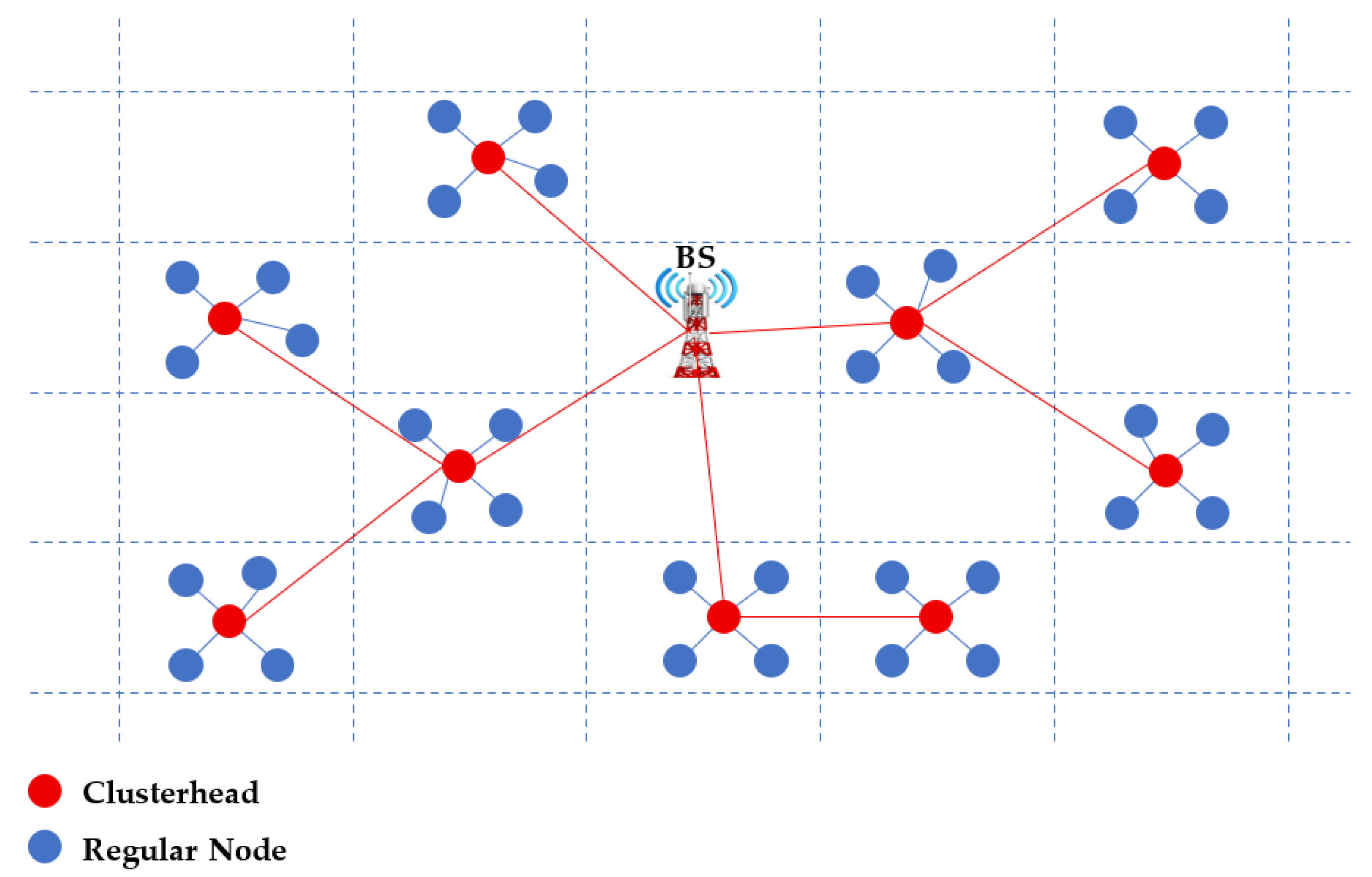
Figure 2.
Effect of weight combinations on FND, HND and LND with BS inside the network.
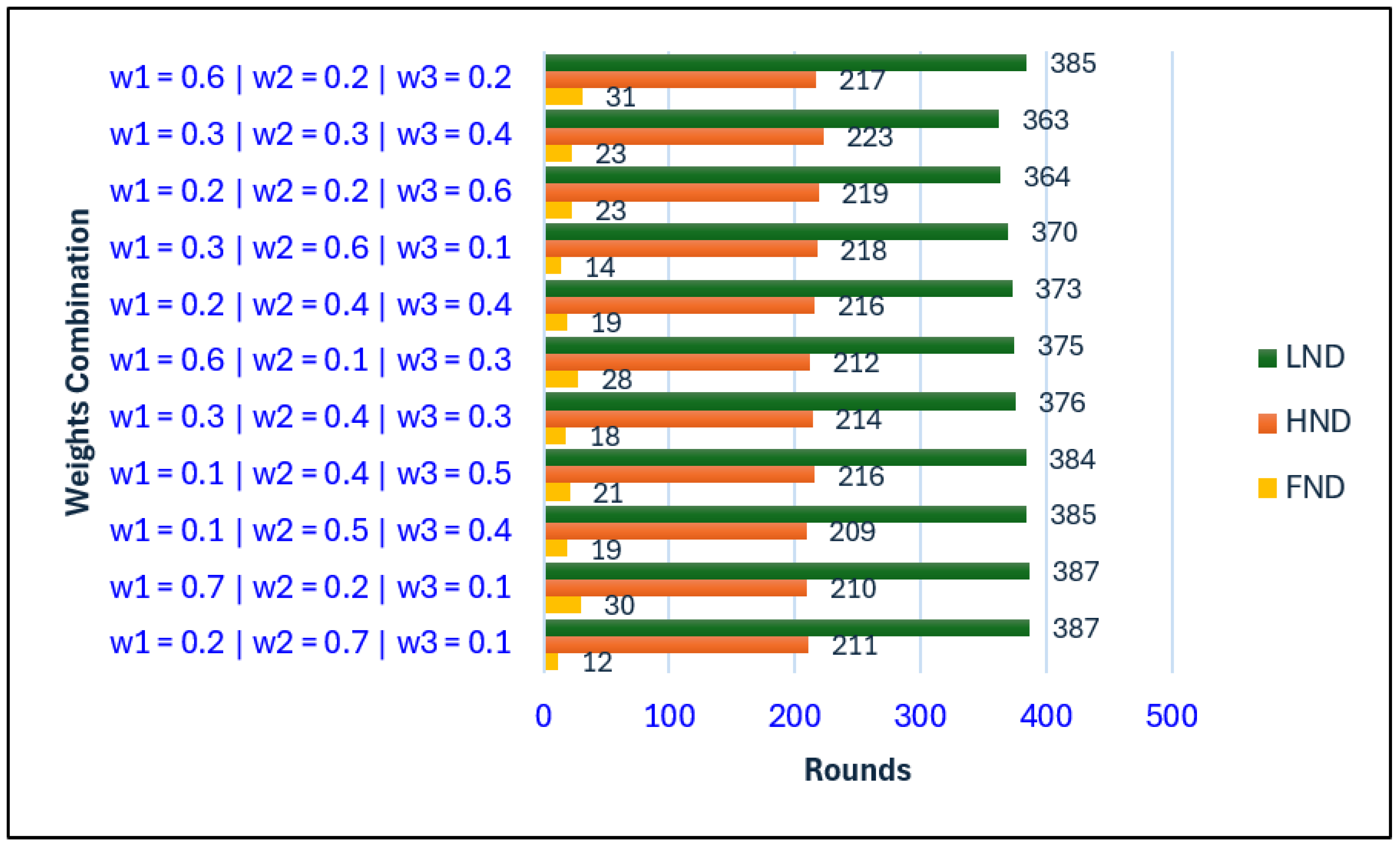
Figure 3.
Effect of weight combinations on data delivery with BS inside the network.
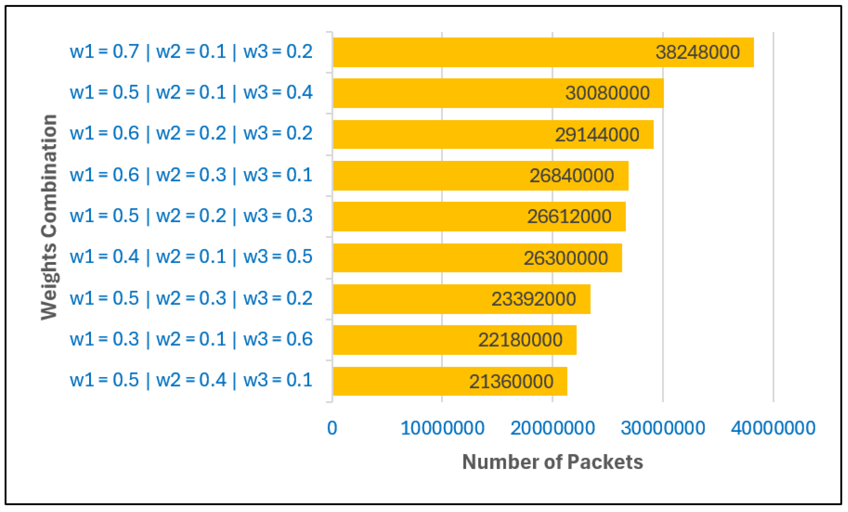
Figure 4.
Effect of weight combinations on live nodes (a), residual energy (b), and CFI (c) with BS inside the network.
Figure 4.
Effect of weight combinations on live nodes (a), residual energy (b), and CFI (c) with BS inside the network.
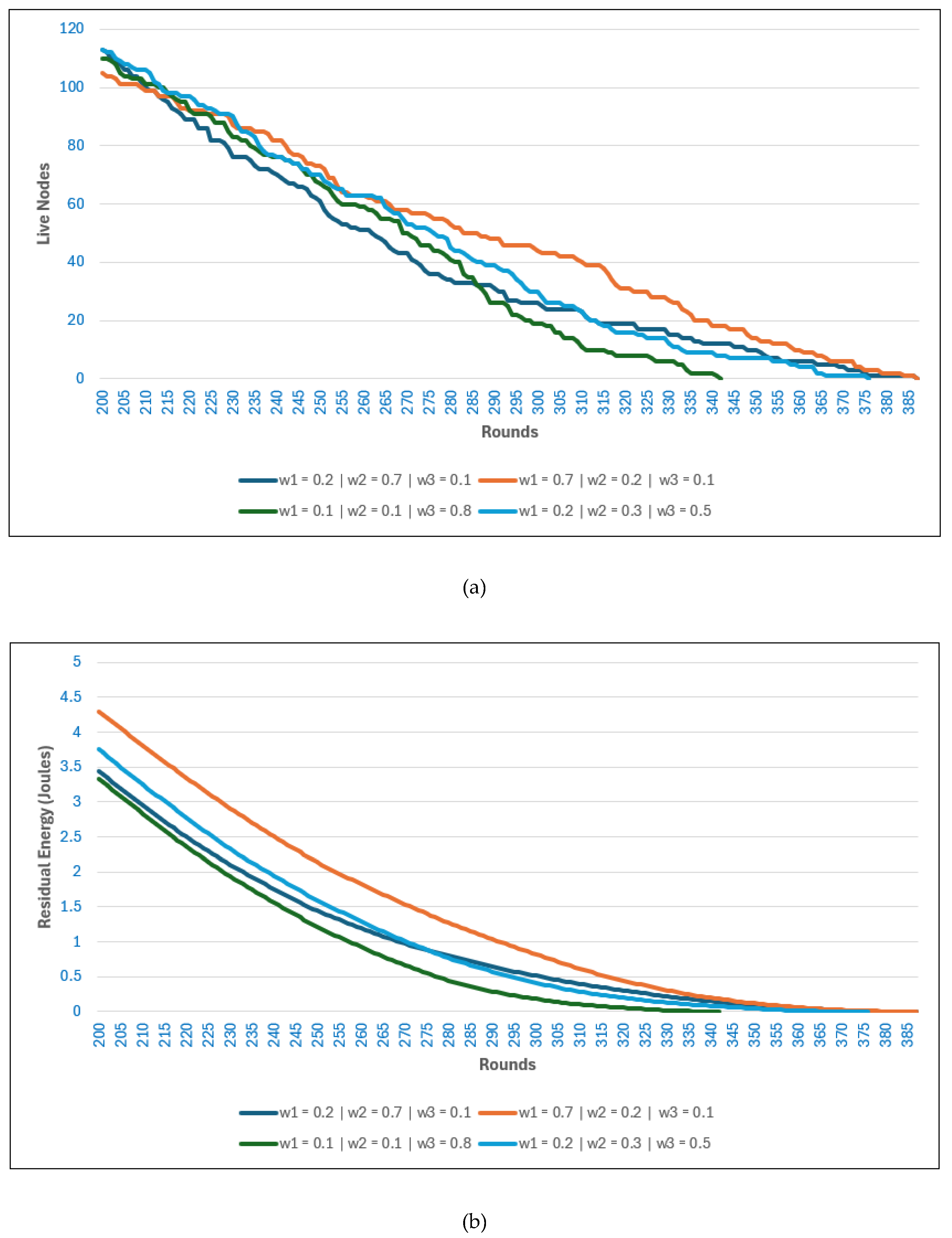
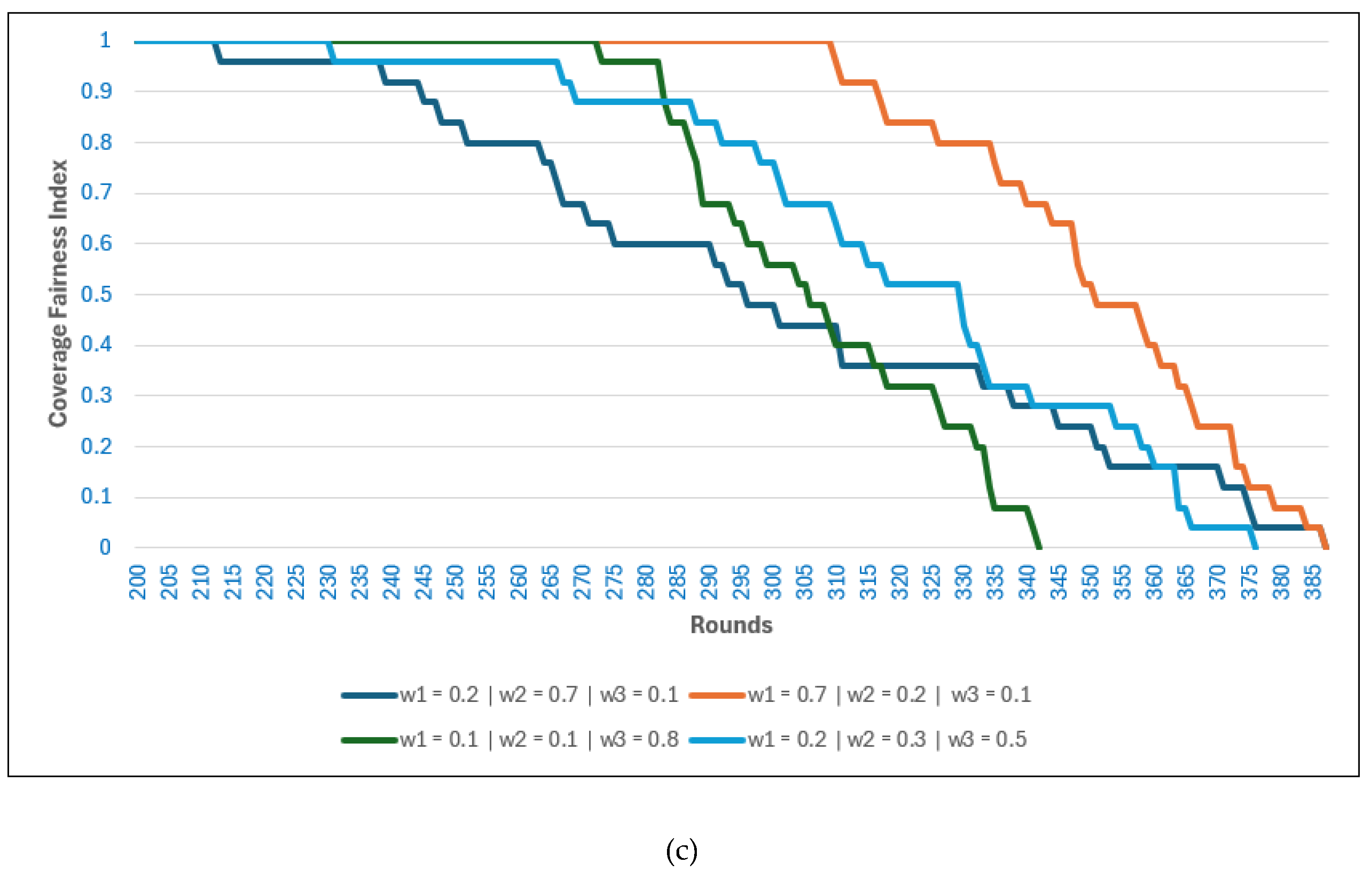
Figure 5.
Effect of weight combinations on FND, HND and LND with BS outside the network.
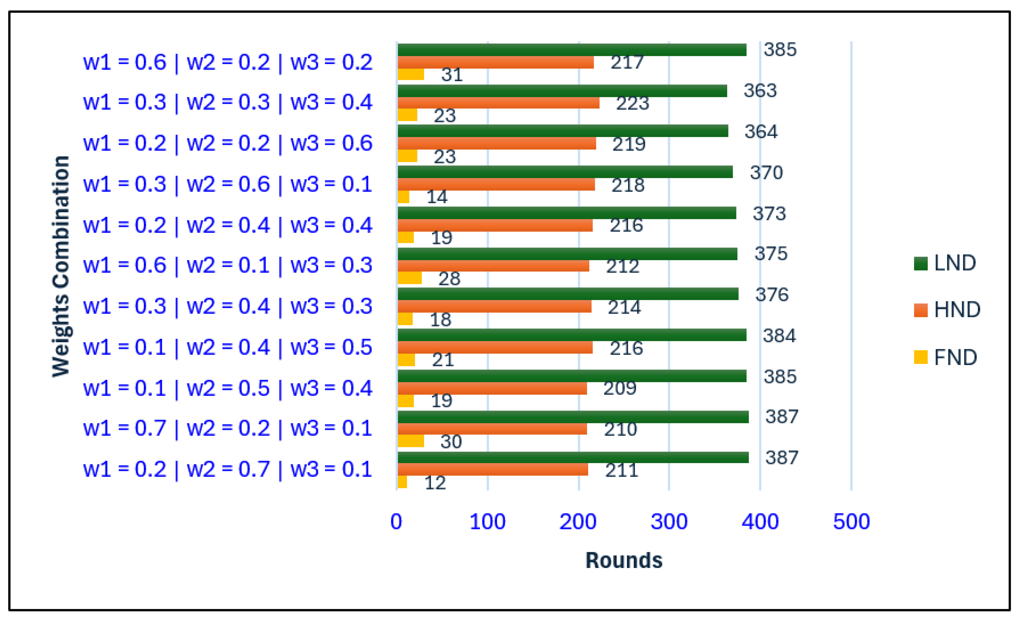
Figure 6.
Effect of weight combinations on data delivery with BS outside the network.
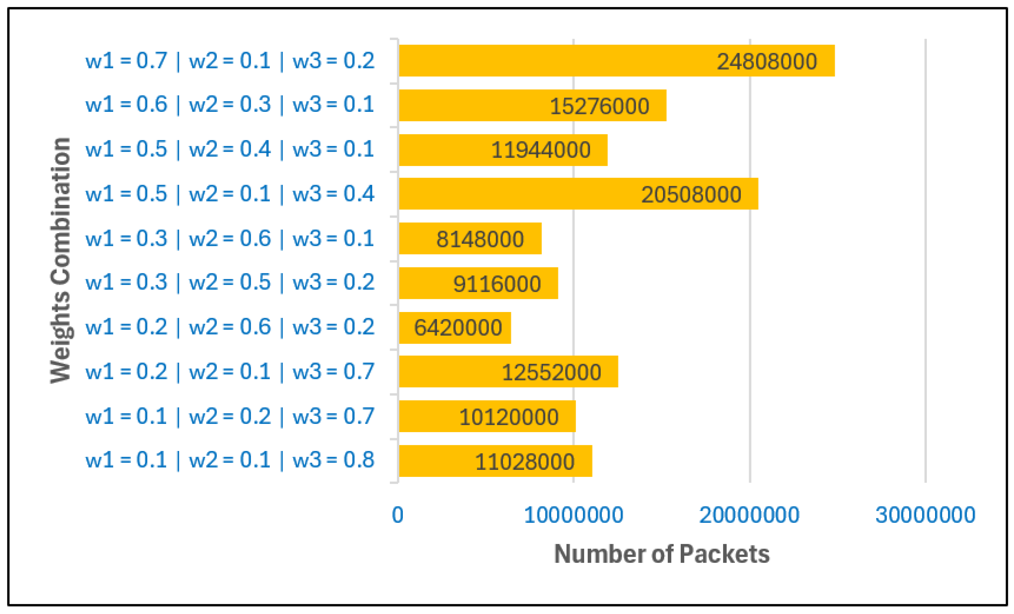
Figure 7.
Effect of weight combinations on live nodes (a), residual energy (b), and CFI (c) with BS outside the network.
Figure 7.
Effect of weight combinations on live nodes (a), residual energy (b), and CFI (c) with BS outside the network.
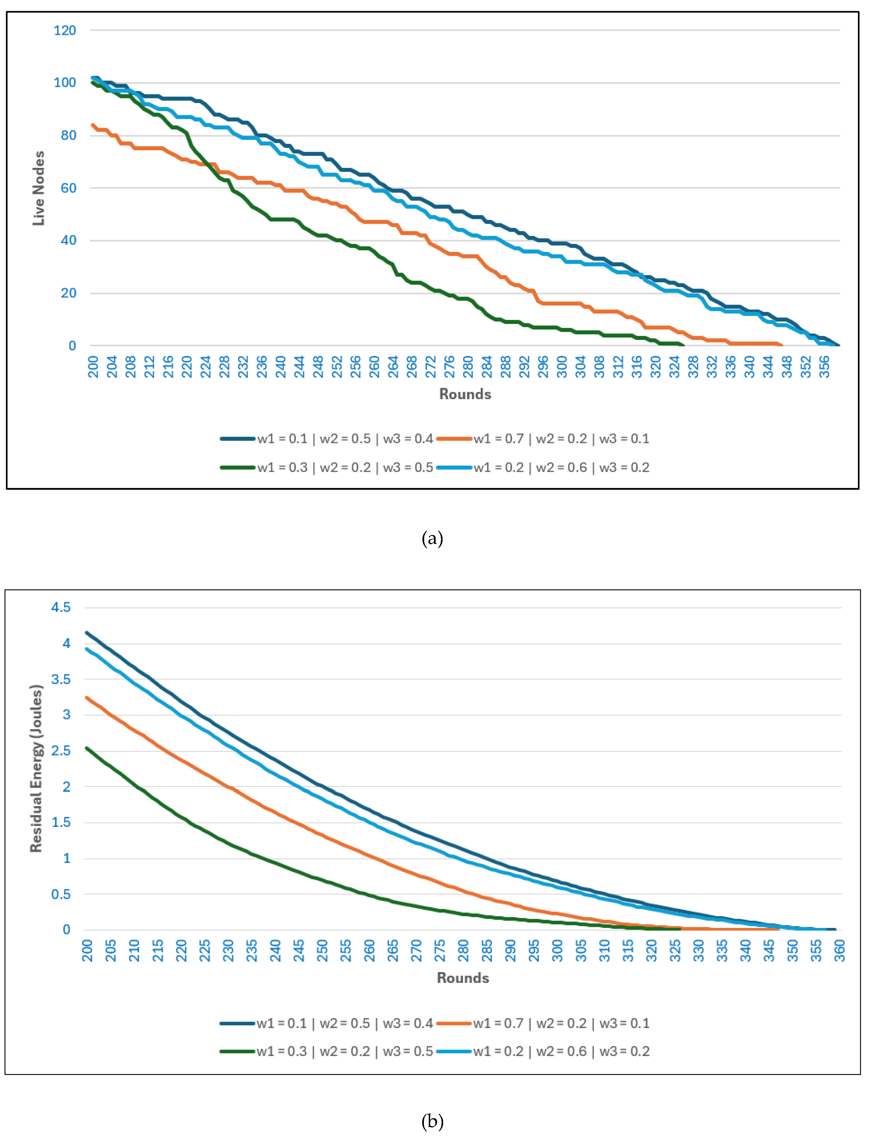
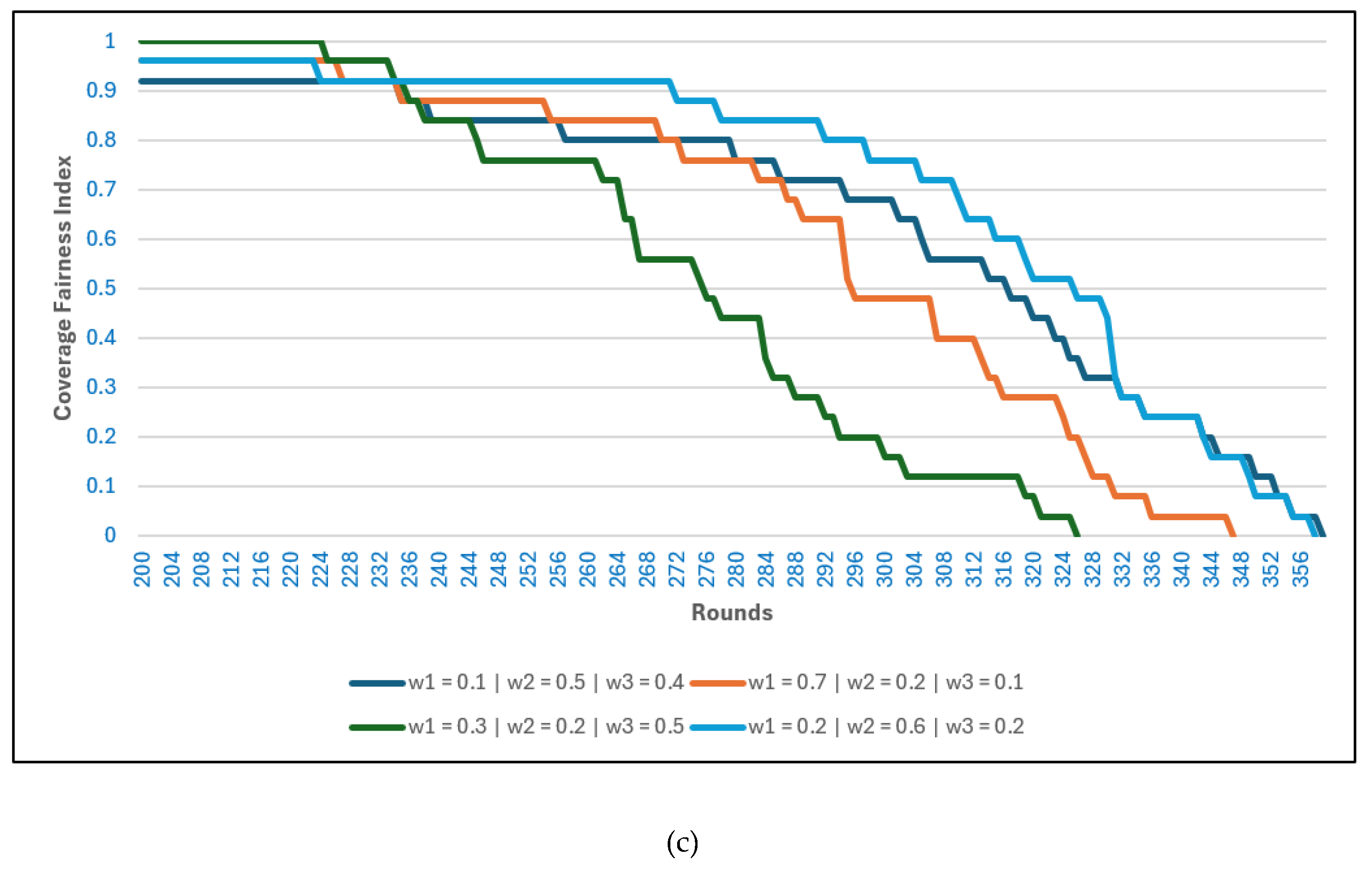
Figure 8.
Comparison of FND, HND, and LND across different routing protocols with BS inside (a) and outside (b) the network.
Figure 8.
Comparison of FND, HND, and LND across different routing protocols with BS inside (a) and outside (b) the network.
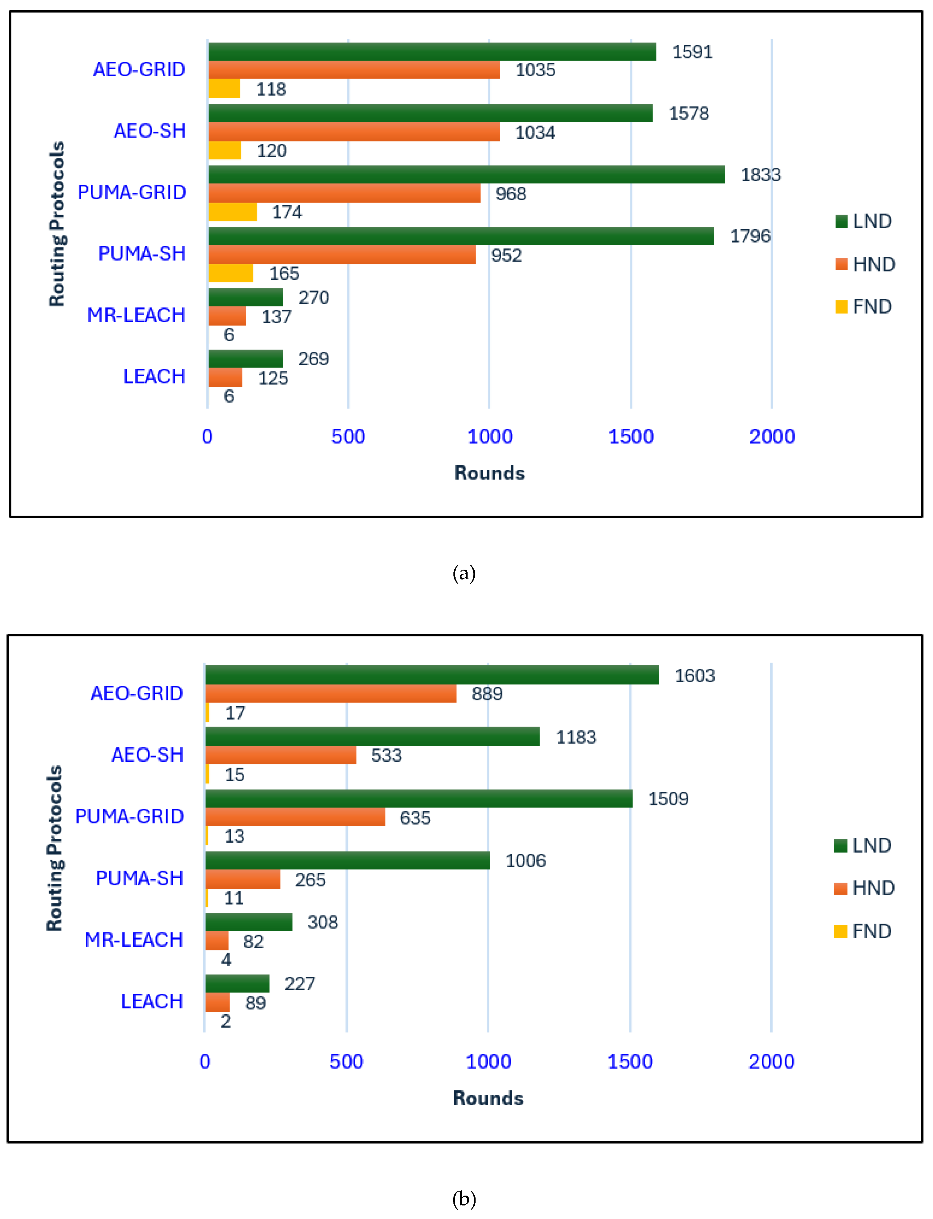
Figure 9.
Comparison of the number of packets delivered to the base station across different routing protocols with BS inside (a) and outside (b) the network.
Figure 9.
Comparison of the number of packets delivered to the base station across different routing protocols with BS inside (a) and outside (b) the network.
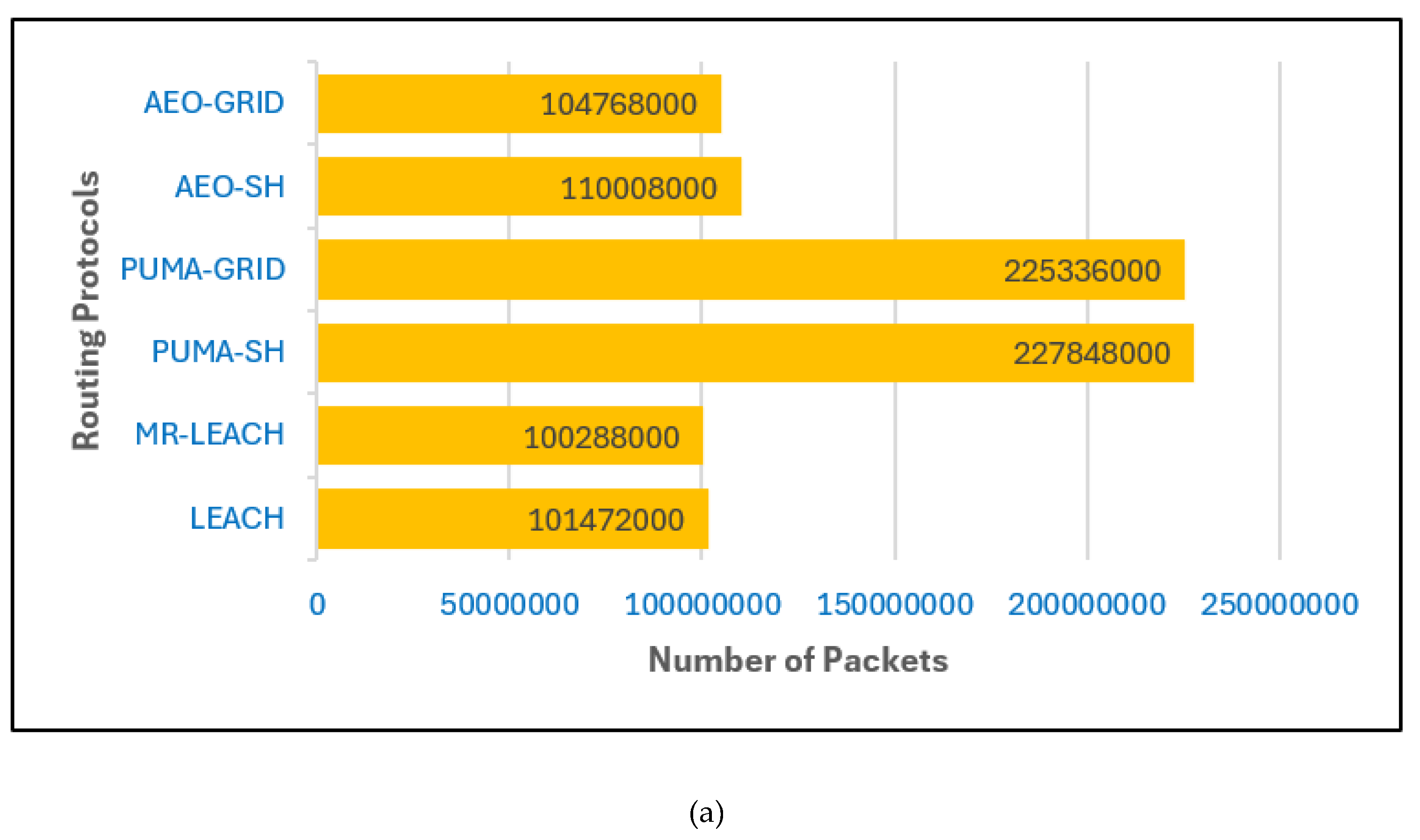

Figure 10.
Comparison of the number of live nodes across different routing protocols with BS inside (a) and outside (b) the network.
Figure 10.
Comparison of the number of live nodes across different routing protocols with BS inside (a) and outside (b) the network.
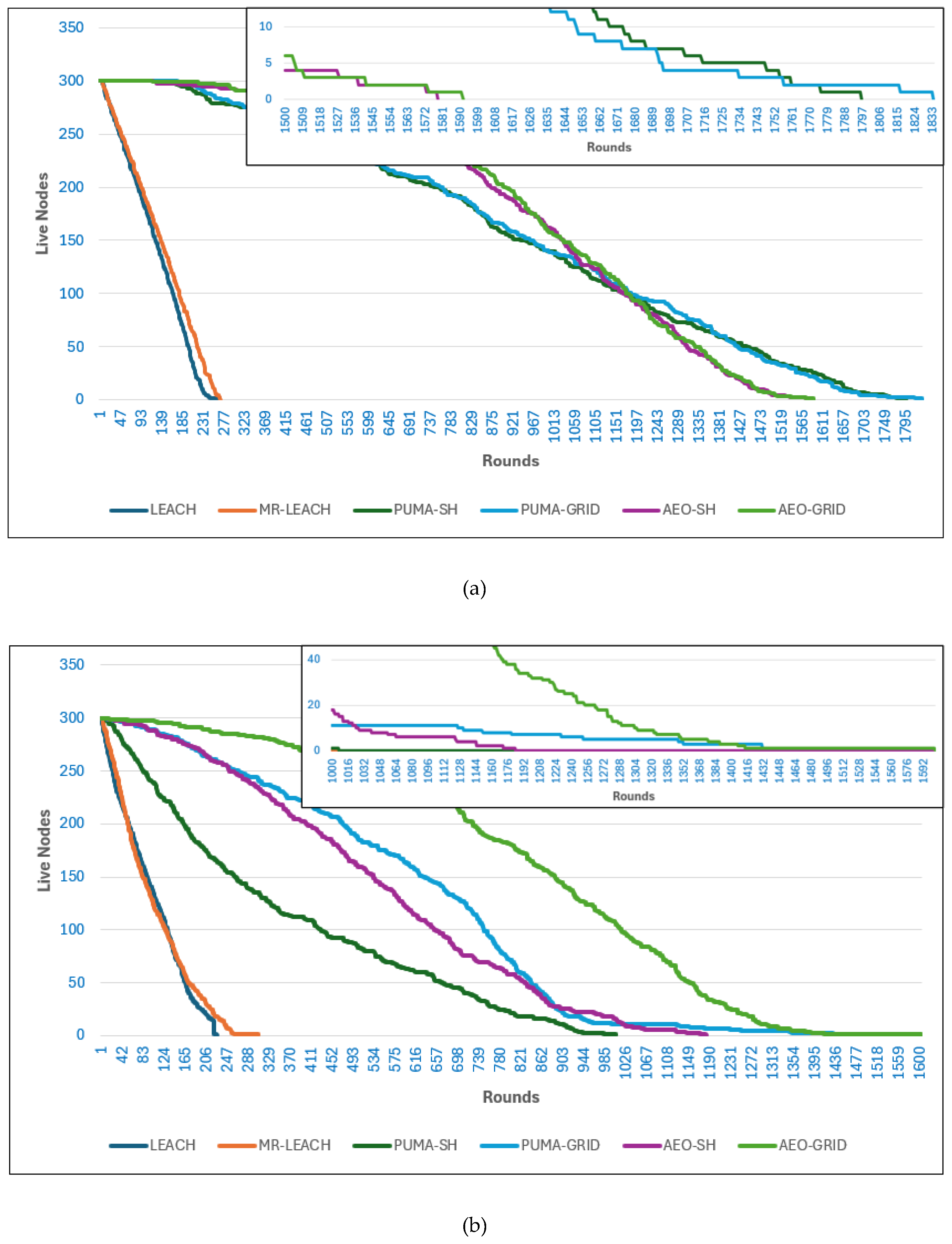
Figure 11.
Residual energy comparison across different routing protocols with BS inside (a) and outside (b) the network.
Figure 11.
Residual energy comparison across different routing protocols with BS inside (a) and outside (b) the network.
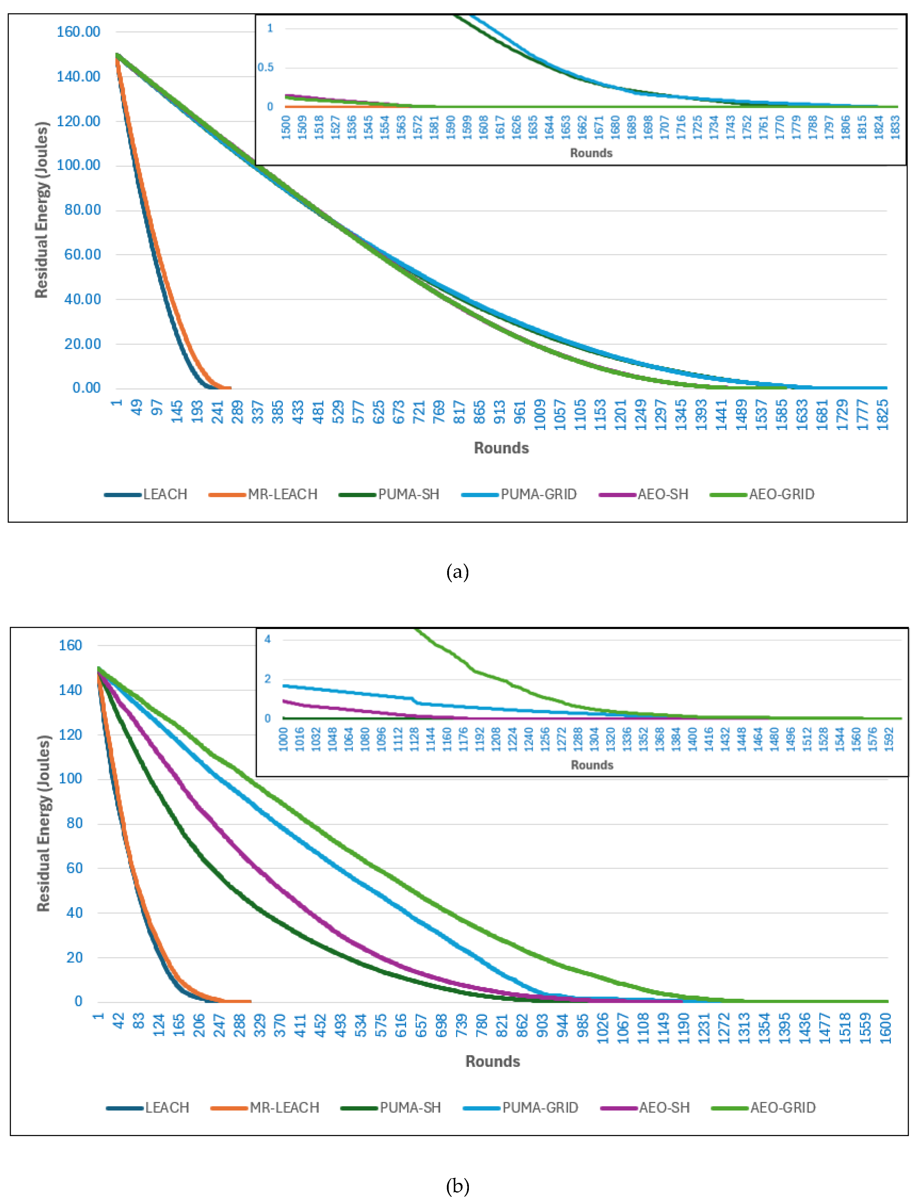
Figure 12.
Comparison of control packet overhead across different routing protocols with BS inside (a) and outside (b) the network.
Figure 12.
Comparison of control packet overhead across different routing protocols with BS inside (a) and outside (b) the network.
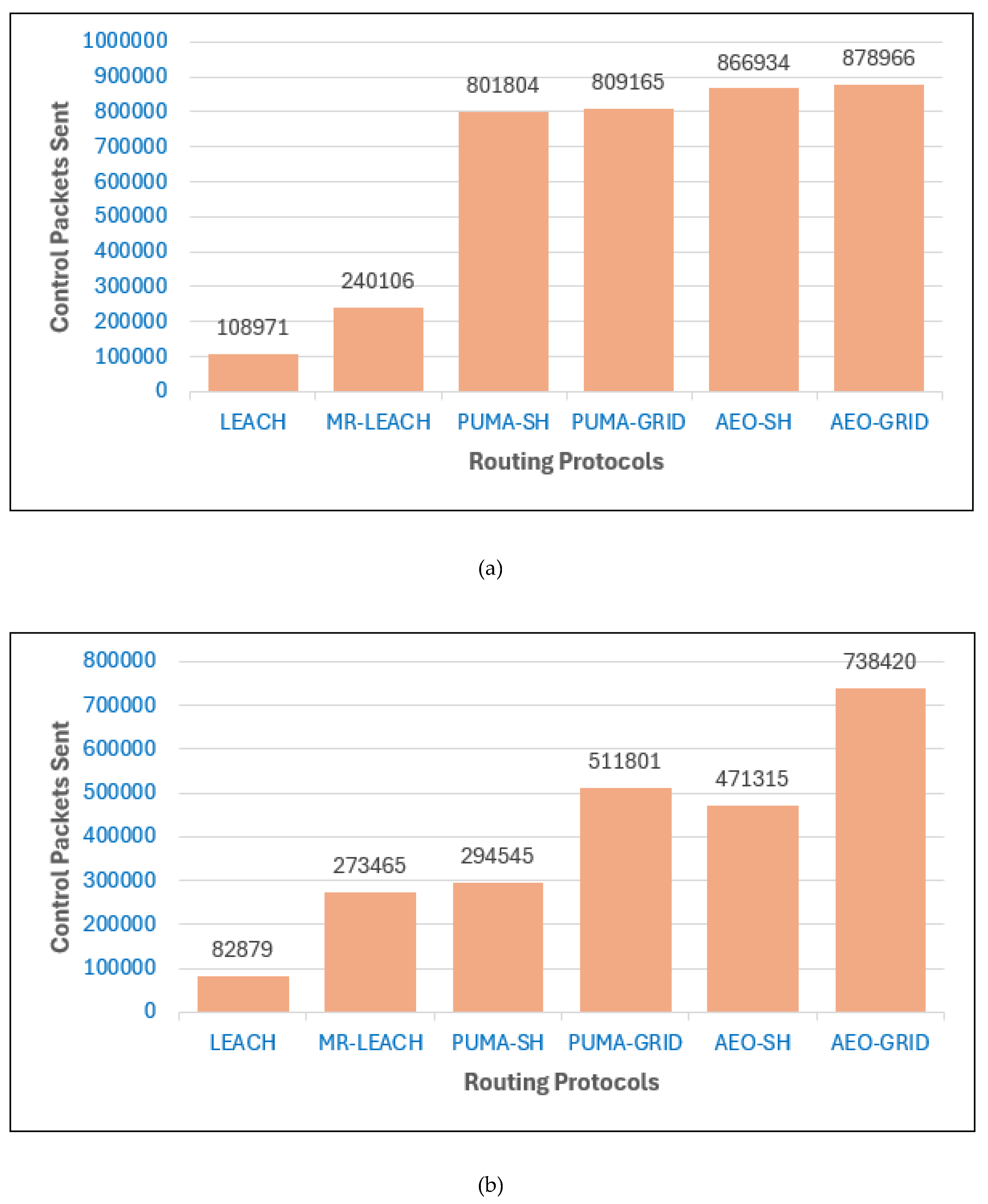
Figure 13.
Network lifetime in terms of the last round sustaining different Coverage Fairness Index (CFI) thresholds for PUMA-GRID and AEO-GRID, with BS inside (a) and outside (b) the network.
Figure 13.
Network lifetime in terms of the last round sustaining different Coverage Fairness Index (CFI) thresholds for PUMA-GRID and AEO-GRID, with BS inside (a) and outside (b) the network.
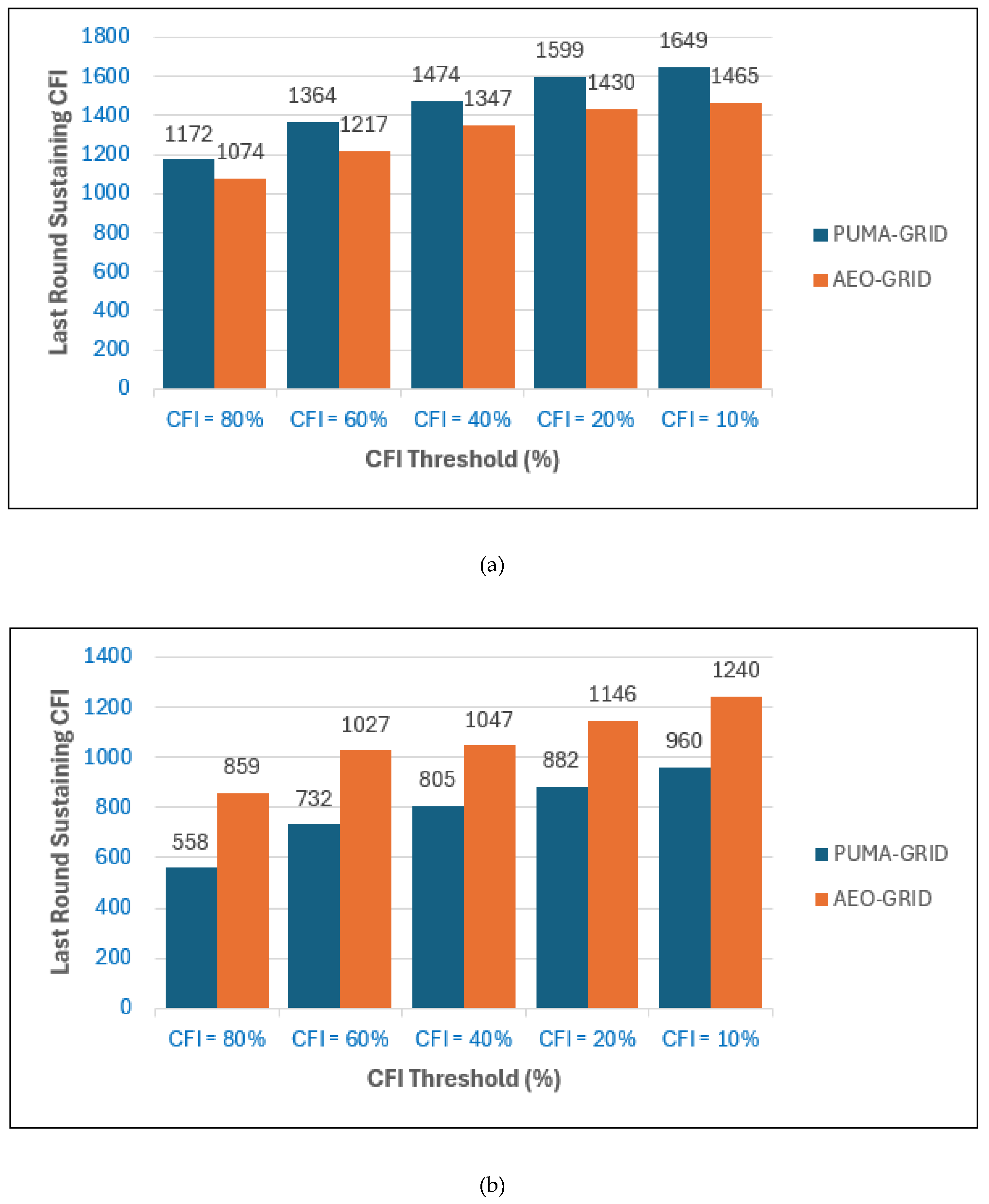

Table 1.
Comparison of clustering protocols in WSNs.
| Protocol | CH Selection method | Parameters Considered |
Routing Type |
|---|---|---|---|
| AEOWSNC | AEO | Distance node → CH; Distance CH → BS | Single-hop |
| SHO-CH | Hyenas | Residual energy; Distance node → CH; Distance CH → BS |
Multi-hop Single-hop |
| AVOACS | African Vulture | Residual energy; Distance node → CH; Distance CH → BS; Communication Mode Decider |
Single-hop |
| EEM-LEACH-ABC | ABC | Residual energy; Distance → BS |
Multi-hop Single-hop |
| BDA | Dragonfly | Residual energy; Distance → BS; Neighborhood degree |
Multi-hop Single-hop |
| KPSOFL | K-means + PSO | Residual energy; Distance → BS; Distance to centroid |
Single-hop |
Table 2.
Simulation parameters for optimal PUMA-GRID weight selection.
| Simulation Parameters | Values/Ranges |
|---|---|
| Network Size | |
| BS Position | (0, 0), (50, 50) |
| Number of Nodes | |
| Node’s Initial Energy | |
| Percentage of Clusterheads | |
| Packet Size | |
| ) | |
| Grid Size |
Table 3.
Simulation parameters for comparing routing protocols.
| Simulation Parameters | Values/Ranges |
|---|---|
| Network Size | |
| BS Position | (0, 0), (100, 100) |
| Number of Nodes | |
| Node’s Initial Energy | |
| Percentage of Clusterheads | |
| Packet Size | |
| ) | |
| Grid Size | |
| 0.5–0.7 | |
| 0.1–0.3 | |
| 0.2–0.3 |
Disclaimer/Publisher’s Note: The statements, opinions and data contained in all publications are solely those of the individual author(s) and contributor(s) and not of MDPI and/or the editor(s). MDPI and/or the editor(s) disclaim responsibility for any injury to people or property resulting from any ideas, methods, instructions or products referred to in the content. |
© 2025 by the authors. Licensee MDPI, Basel, Switzerland. This article is an open access article distributed under the terms and conditions of the Creative Commons Attribution (CC BY) license (http://creativecommons.org/licenses/by/4.0/).
Copyright: This open access article is published under a Creative Commons CC BY 4.0 license, which permit the free download, distribution, and reuse, provided that the author and preprint are cited in any reuse.


