Latin Grid Generation Algorithm, Exact Counting Framework, Isomorphic Polyn-Omial Determination Algorithm, and Exact Solution Algorithm for Pending Filling

1. Introduction

The Latin grid was introduced by Euler in a 1782 paper [1], and its generation and counting have remained long- standing problems in combinatorial mathematics. Valiant’s groundbreaking work proved that the product and summation of 0-1 matrices are #P-complete [2], while subsequent proofs showed that precise counting of Latin grids is also #P-complete [3], indicating their extreme difficulty. Most researchers use Monte Carlo sampling methods [4] to approximate the number of Latin grids. The inability to achieve precise counting primarily stems from limitations in generation algorithms, including random generation, swapping method, recursive construction, and group-theoretic construction [3], which can only produce specific types like cyclic Latin grids or generate duplicates due to inherent uncertainty in generation strategies. Due to these algorithmic constraints, the maximum order of Latin grids calculated so far is n=11 [5]. BD McKay and colleagues compiled precise counts for various orders and classifications of Latin grids [6]. This paper’s algorithm leverages the algebraic structural property of square grids where row-column swaps remain invariant, enabling generation of all N×N Latin grids without repetition. Benefiting from this unique generative characteristic, we further propose a framework for precise counting of Latin grids. The specific counting formula is still under derivation and may be presented in future versions.

An n-order Latin square is an n×n matrix where each row and column contains exactly n symbols, with each symbol appearing exactly once. In the multiplication table of an n-order quasi-group (Q, °), the element at position (a, b) represents the product a ° b. If we define L= mab where mab = a ° b, then the resulting array L forms an n- order Latin square. Conversely, any binary operation derived from such a Latin square constitutes a quasi-group on the set Q. Thus, Latin squares and quasi-groups are mathematically equivalent in structure. In the paper by NA Collins et al., it is explicitly stated that Latin grid isomorphism is equivalent to group homomorphism [7].Marty J. Wolf categorized Latin grid isomorphism (group homomorphism) into $NNC\left(\mathrm{polylog}\right)$, where NNC represents a new non-deterministic complexity class introduced by them as a quantifiable resource for non-deterministic computations. This classification uses a finite number of non-deterministic gates to derive $NNC\left(\mathrm{polylog}\right)$ from NC circuits, serving as a candidate to separate NC and NP. It also demonstrates that $NNC\left(\mathrm{polylog}\right)\subseteq \mathrm{DSPACE}\left(\mathrm{polylog}\right)$[8].NA Collins et al. advanced this classification by showing that group homomorphism $\in {\exists }^{{log}^{2}n}{\mathrm{AC}}^0(DTISP(polylog\left(n\right),logn))$, and demonstrated that group homomorphism, Steiner triple system isomorphism, pseudo-Steiner triple system graph isomorphism, Latin grid graph isomorphism, and Steiner $(t,t+1)$ designs share the same upper bound. They also improved the previous upper bound for isomorphism problems: ${\exists }^{{log}^{2}n}\mathrm{L}\cap {\exists }^{{log}^{2}n}\mathrm{FOLL}\subseteq \mathrm{quasiFOLL}$ [7].

Many isomorphism problems, including Latin Grid Isomorphism, Quasi-Group Isomorphism, Group Isomorphism, Graph Isomorphism, and Steiner’s Design Isomorphism Test, are considered candidates for the intermediate zone between P-problems and NP-complete problems. A Chattopadhyay et al. demonstrated that graph isomorphism cannot be $\mathrm{Not}{\mathrm{AC}}^0-\mathrm{Reducible}$ to quasi-group isomorphism and group isomorphism. Graph isomorphism is more challenging than quasi-group and group isomorphism unless all three can be solved in polynomial time [9]. Subsequently, M. Levet extended this result to Latin Grid Isomorphism [10], while Gary L. Miller [11] adapted Tarjan’s technique to Latin Grid Isomorphism and Quasi-Group Isomorphism, enabling determination of isomorphism between two n-order quasi-groups within $n^{logn}$ steps. Latin Grid Isomorphism, Quasi-Group Isomorphism, and Group Isomorphism have been studied for decades due to their close connections with computational complexity theory, cryptography, computational group theory, and algebraic complexity theory [12,13]. The following section presents a polynomial-time algorithm for Latin Grid Isomorphism.

The Latin Square Filling Problem (LPFP) is a classic NP-complete problem [14]. Since its introduction, it has become one of the most significant challenges in theoretical computer science, attracting extensive research from mathematicians and yielding numerous algorithms. The classical solutions for LPFP include backtracking algorithms and dance chain algorithms. This paper presents a novel generation-based algorithm for efficient and accurate solution computation. Unlike conventional approaches, our algorithm not only guarantees all possible solutions but also demonstrates computational efficiency. Furthermore, the algorithm remains continuously optimized for enhanced performance, with new versions to be released subsequently.

2. Basic Terminology

Quadrilateral: In any N×N Latin square L, select two pairs of symbols located on opposite diagonals and equidistant from each other, denoted as (a, b) and (c, d). Here, a and b lie on one diagonal, while c and d reside on the opposite diagonal. The ordered pair formed by these numbers ((a, b), (c, d)) is called a quadrilateral. When performing arbitrary row-column swaps on a Latin square L to obtain a new square L’, the diagonal structure remains unchanged. This means the quadrilateral serves as an invariant under row-column operations in Latin squares. These four types of quadrilaterals maintain their identity under row-column swaps, making them algebraic invariants equivalent to mathematical operations involving such transformations.

Diagonal Symmetry: In the four-square grid ((a, b), (c, d)), where a and b lie on one diagonal while c and d form another, the diagonal distance between a and b equals that between c and d. This ensures that any symbol in the grid aligns with its adjacent symbols either horizontally or vertically. When symbol a undergoes transposition to symbol b, symbol c will symmetrically correspond to symbol d. From this, we derive four types of four-square grids: Type I ((a, b), (c, d)), Type II ((a, b), (d, c)), Type III ((a, a), (c, c)), and Type IV ((a, a), (c, d)).

Square grid element: The basic element that constitutes a square grid, namely two pairs of symbols located on the opposite diagonals and at equal distances from each other. Each square grid has and only one Four square quanta.

Main and Secondary Lines: In any $N\times N$ Latin square, there are two diagonals of the longest geometric length $n\sqrt{2}$ (where n is the side length of the Latin square). One is called the main line if all symbols are the same, and the other is called the secondary line.

Mainline Normative Type: Let L be an N×N Latin square (where each row and column in L is a permutation of the set 1, 2,..., N). If there exists a row-column swapping transformation T (a combination of row and column transformations) such that the transformed Latin square L’ = T(L) satisfies the following conditions:

1. The elements on the main diagonal are L’ i, i = N, for all i = 1,2,..., N;

2. If each row and column are still permutations of 1,2,..., N, then L’ is called a line-oriented regular Latin grid.

For the fourth type of square grid under the main-line specification framework in N×N Latin squares, a primary line is selected (where all symbols on the main diagonal are identical, denoted as K). Two symbols x and y positioned symmetrically on both sides of this main line form a pair (x: y). All pairs must satisfy the following properties.

• The total number of groups is $(N-1)+(N-2)+\dots +2+1={\displaystyle \frac{N(N-1)}{2}}$;
• Number of symbol occurrences: in all pairs, the total number of symbols is N;
• Invariance: the group is invariant under the exchange of Latin square rows and columns.

Pair structure: If two pairs can be obtained by symbol substitution, then the pair structures are identical. There are only two pair structures (a: a) and (a: b).

Collection of pairs: the collection formed by all pairs of groups in which any symbol is the main line (the same symbol on the diagonal).

Pairing set structure: If the pairing set of two Latin squares can be obtained from each other by symbol substitution, and the number of partition parts of the pairing is the same, and the symbol composition of each part is completely identical, then they are said to have the same pairing set structure.

Group elements: Two symbols that are symmetric about the main line are the basic elements that make up the group.

Group: Set two pairs of groups. If their pairs are located in the same row or column, they are called pairs of groups, that is, they are in the same row and column.${\displaystyle \frac{4(N-2)}{2}}$ (or simplified as $2(N-2)$, where $N\ge 4$)

External group: If two pairs of groups are not located in the same row or column, they are called external groups, that is, their positions in the row and column. There is no specific correspondence. In any N × N Latin square, the number of groups is:$\left(N-3\right)+\left(N-4\right)+\cdots +4+3+2+1(N\ge 4)$

Origin: There are four vertices in the Latin square, two of which are located on the main line, and the other two vertices are located in the region called the origin.

Construction zone: The outermost two rows and two columns of the Latin square, with four vertices at the ends of these two rows and two columns, are called the construction zone, which does not include the outermost two rows and two columns.

Closing area: The two outermost rows and columns of the Latin grid, but not including the starting area.

Start symbol: A number located in the start area is called a start symbol. If symbol a is located in the start area, all symbols a are called start symbols. If both symbol a and b are located in the start area, all symbols a and b are called start symbols.

Non-starting symbol: All symbols that are not located in the starting area are called non-starting symbols.

3. Generating Algorithm

3.1. All N×N Latin Squares Are Generated so That the Rows and Columns Do Not Repeat, and the Generation Is a Unique Latin Square Algorithm

This section gives an algorithm designed based on the invariant property of the exchange structure of the four- dimensional square matrix. Using this algorithm, all N × N Latin squares can be generated, and the exchange of the matrix is not repeated. The generation is a unique Latin square algorithm, and there is no need to check for duplication.

The Latin square is defined as: Let n be a positive integer, and the set S = 1,2,...,n. A N × N matrix L = (Li,j) satisfies:

• For any $i\in \{1,2,\dots ,n\}$, the set $\{L_{i1},L_{i2},\dots ,L_{in}\}=S$ (that is, each row element forms a permutation of S);
• For any $j\in \{1,2,\dots ,n\}$, the set $\{L_{1j},L_{2j},\dots ,L_{nj}\}=S$ (where each column of elements forms a permutation of S) is called the Latin square matrix L of order $N\times N$.

Therefore, we conclude that $L=\left(L_{i,j}\right)$ forms an $N\times N$ Latin square, where $L_{i,j}$ denotes the element at position $i,j$ in the matrix ($i,j\in \{1,2,\dots ,N\}$). For any $k\in \{1,2,\dots ,N\}$, there exist row permutation $\pi$ (a permutation of $\{1,2,\dots ,N\}$) and column permutation $\delta$ (also from $\{1,2,\dots ,N\}$) such that the transformed Latin square $L^{\prime }=\left(L_{i,j}^{\prime }\right)$ satisfies: For all $i\in \{1,2,\dots ,N\}$, it holds that $L_{i,i}^{\prime }=k$. In this case, $L^{\prime }$ is called a "k-line Latin square" – meaning through these permutation operations, all diagonal elements become k. The term "k-line" specifically denotes the canonical form where all diagonal elements are k.

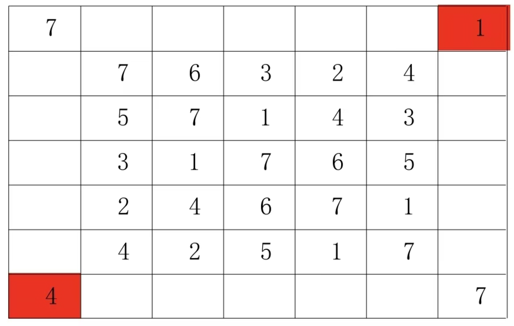
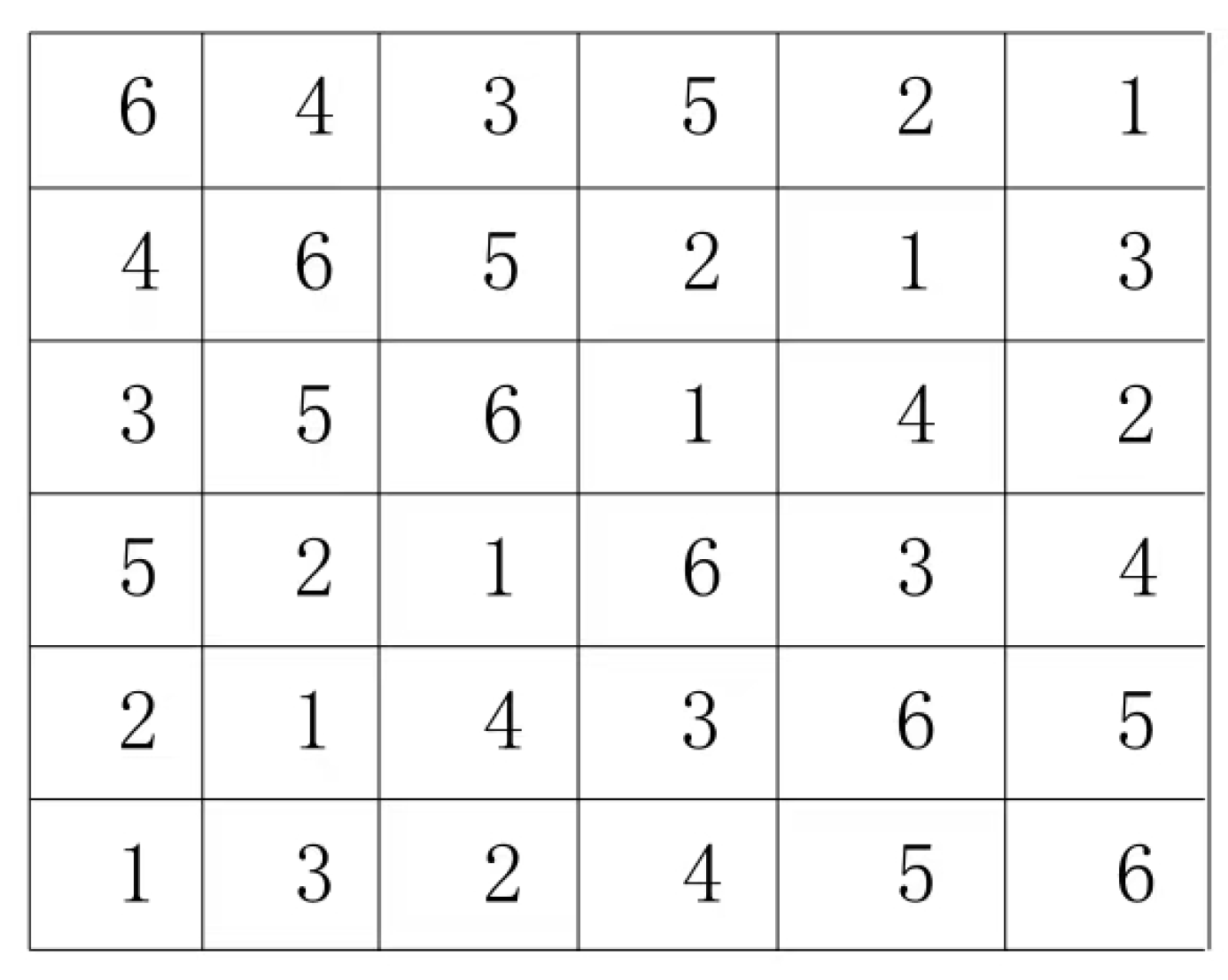
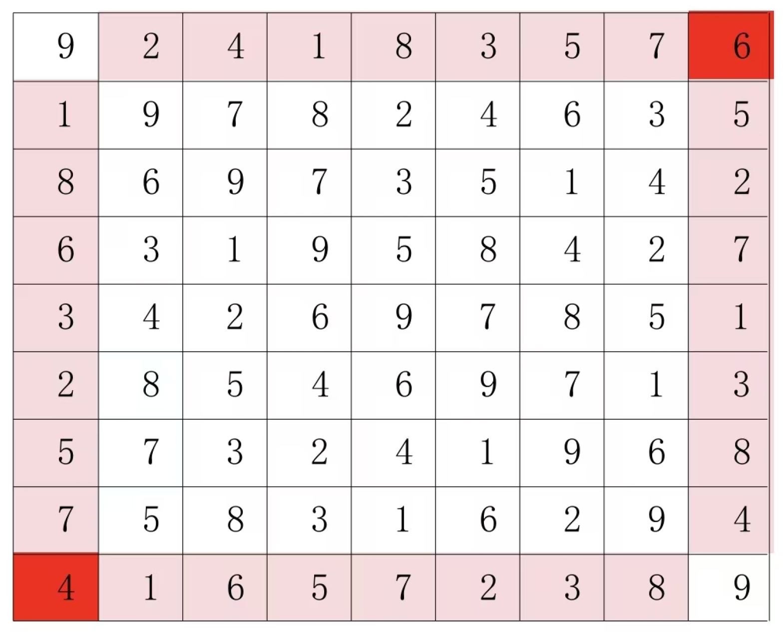
Usually the line with the largest number is taken as the main line. The following example uses a 5 by 5 Latin square.

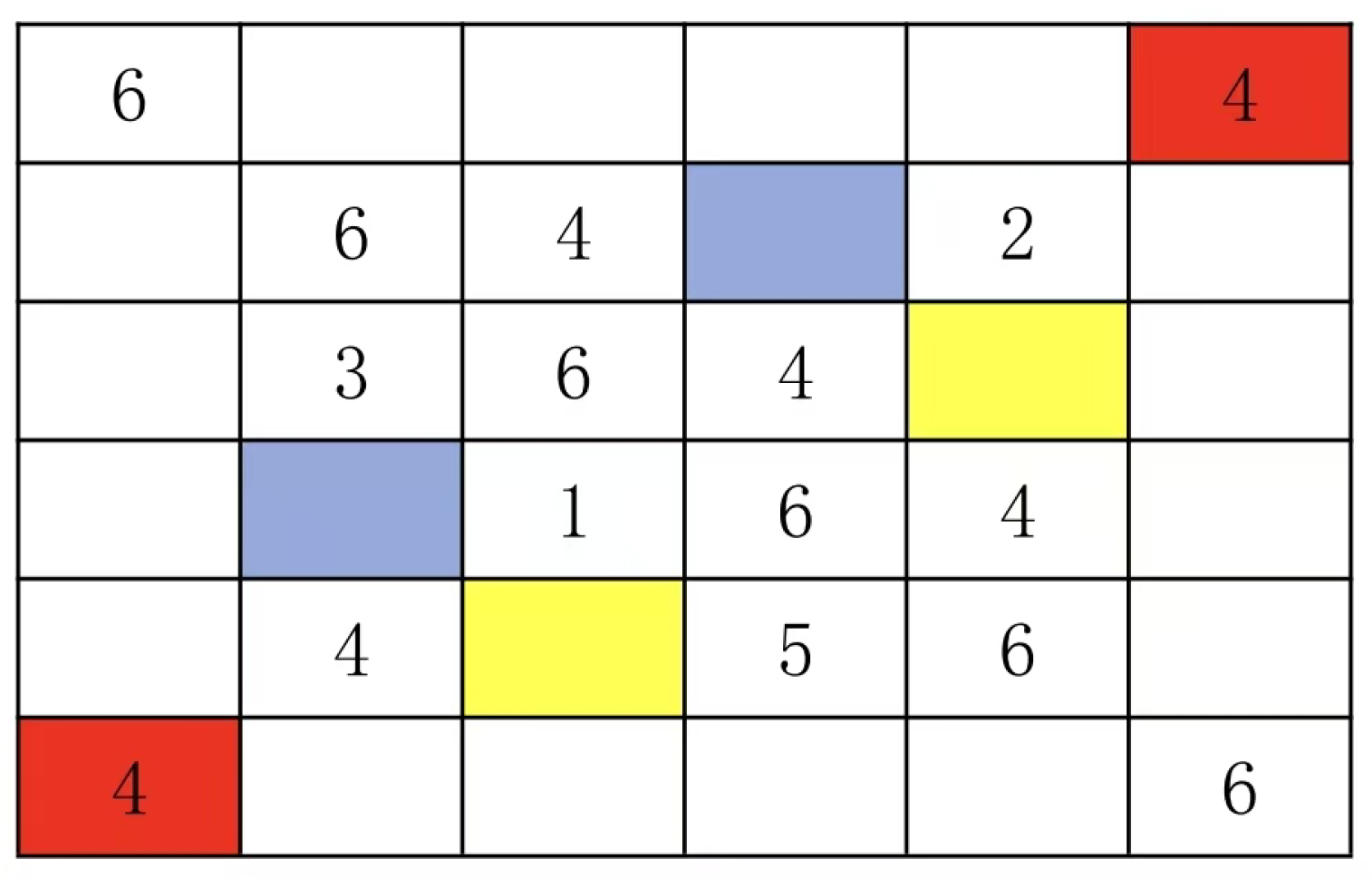
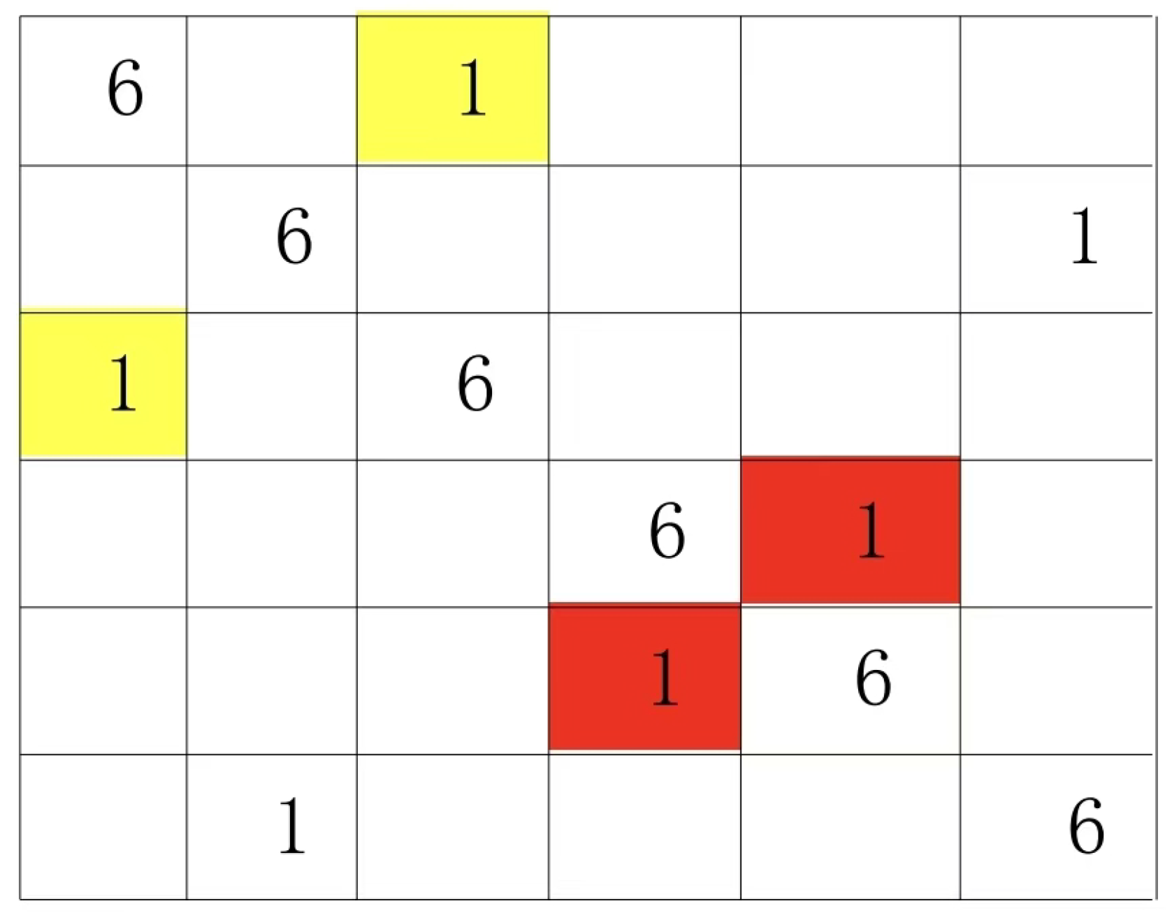
This type of Latin grid, referred to as the mainline specification type in this paper, features paired groups on both sides of its mainline. For example, this Latin grid contains N=5, with a total of 10 paired groups (4+3+2+1= 10). The group configurations are as follows: yellow (1:4), red (4:1), blue (2:3), cyan (2:3), and others include (1:4), (2:3), (1:4), (3:2), (2:3), (4:1), (1:4), (3:2), (2:3), and (1:4). Based on the definition of Latin grids and the mainline specification type, we can derive the following properties of paired groups, which are also known as constraint conditions.

• In all the $N\times N$ Latin squares, the total number of groups is $(N-1)+(N-2)+\cdots +2+1$.
• The total number of all the numbers in the group adds up to N.

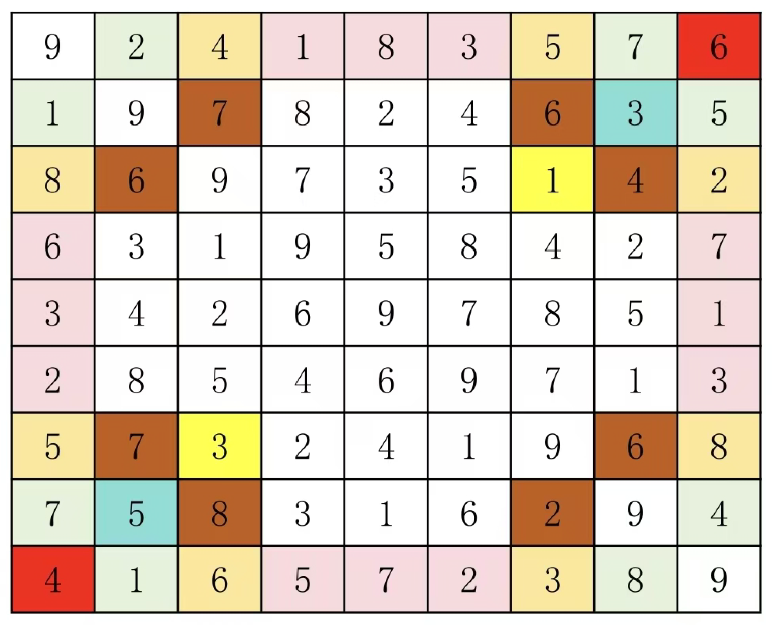
In this context, a pair group essentially represents the fourth type of square grid. Specifically, it refers to a pair within square grids where all numbers in the pair are identical. For instance, in the 5×5 Latin grid shown above, the pair group (1:4) corresponds to the square grid (4, 1) and (5,5). This principle holds true for all N×N Latin grids. Since square grids maintain their mathematical structure under column-row permutation, the pair group retains its structural integrity even after such transformations.

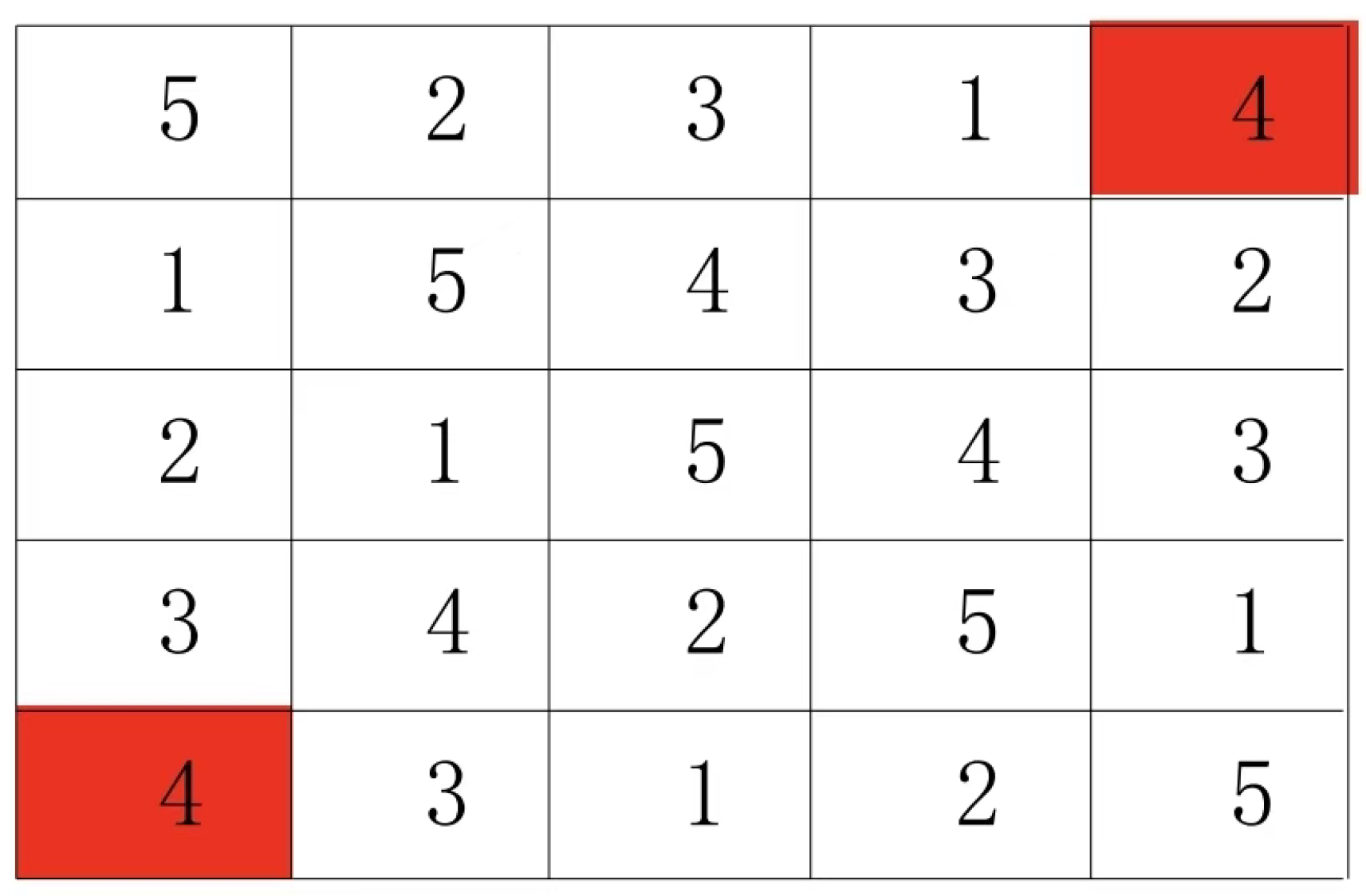
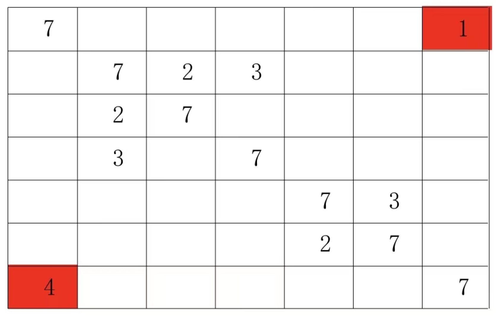
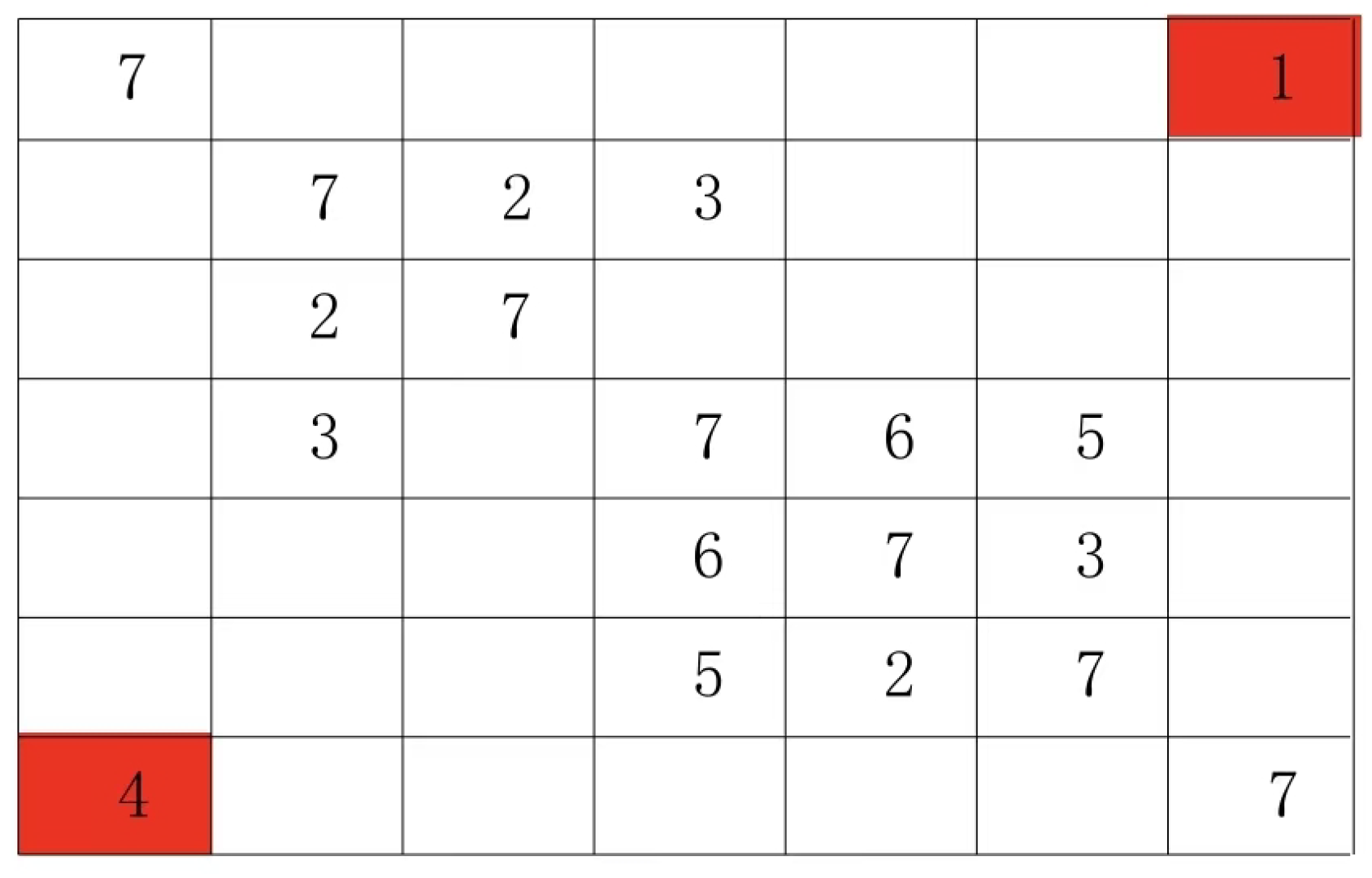
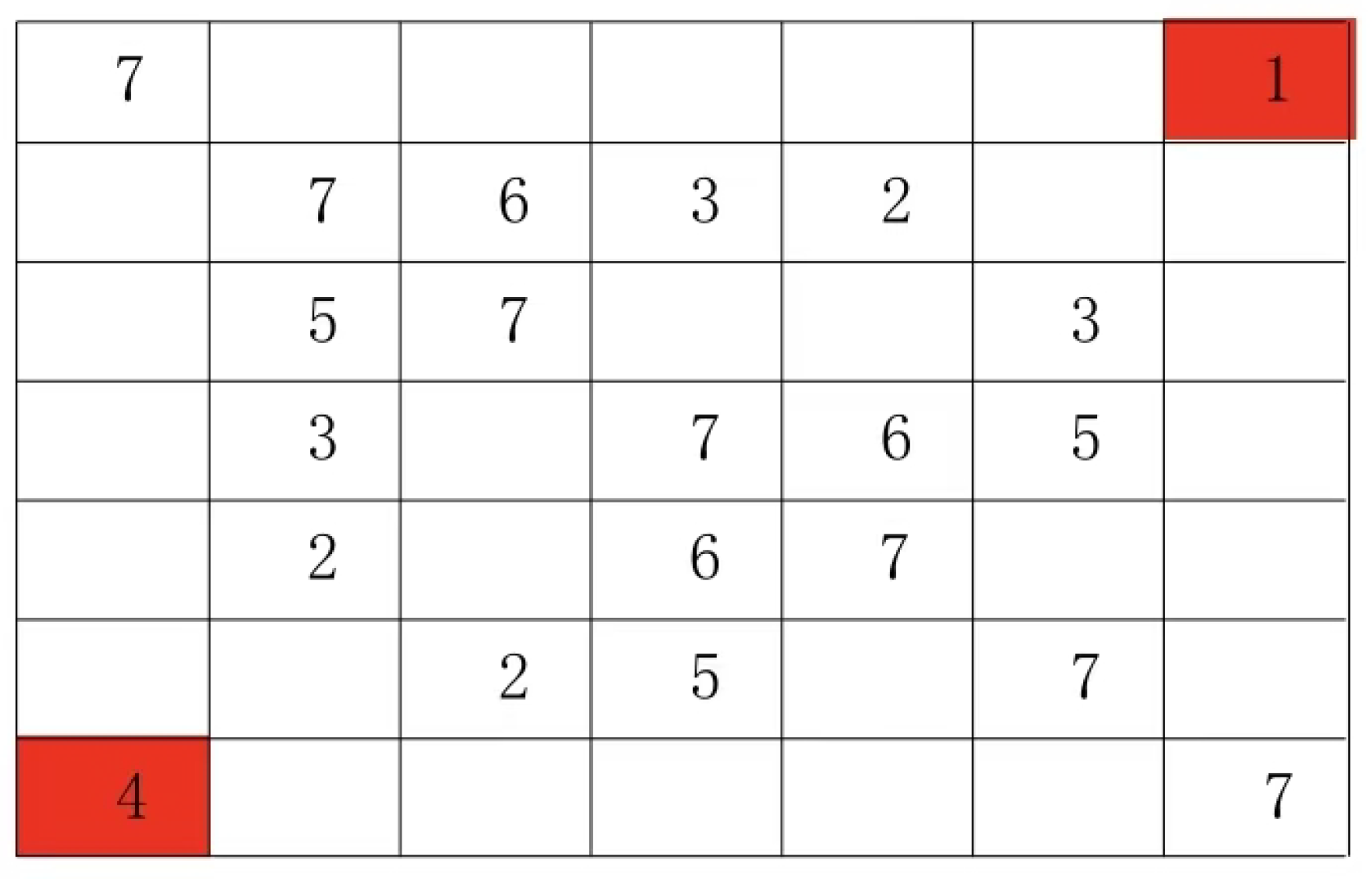
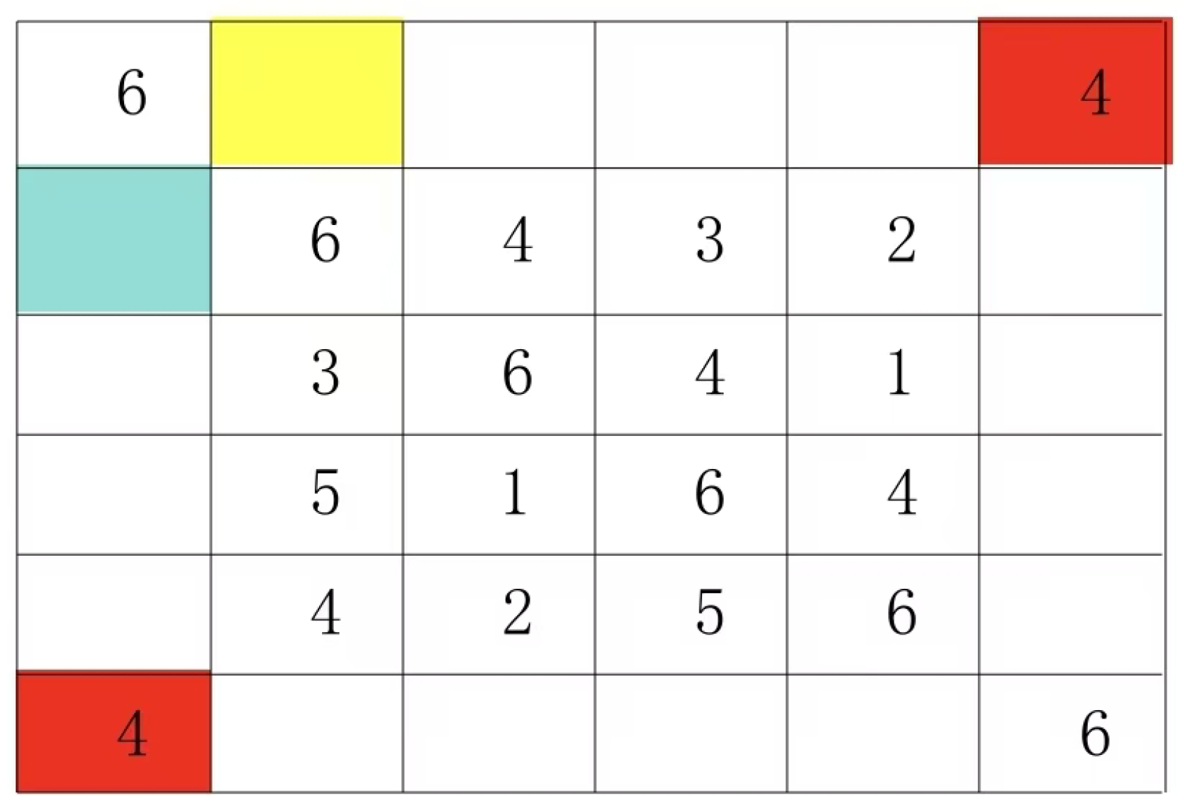
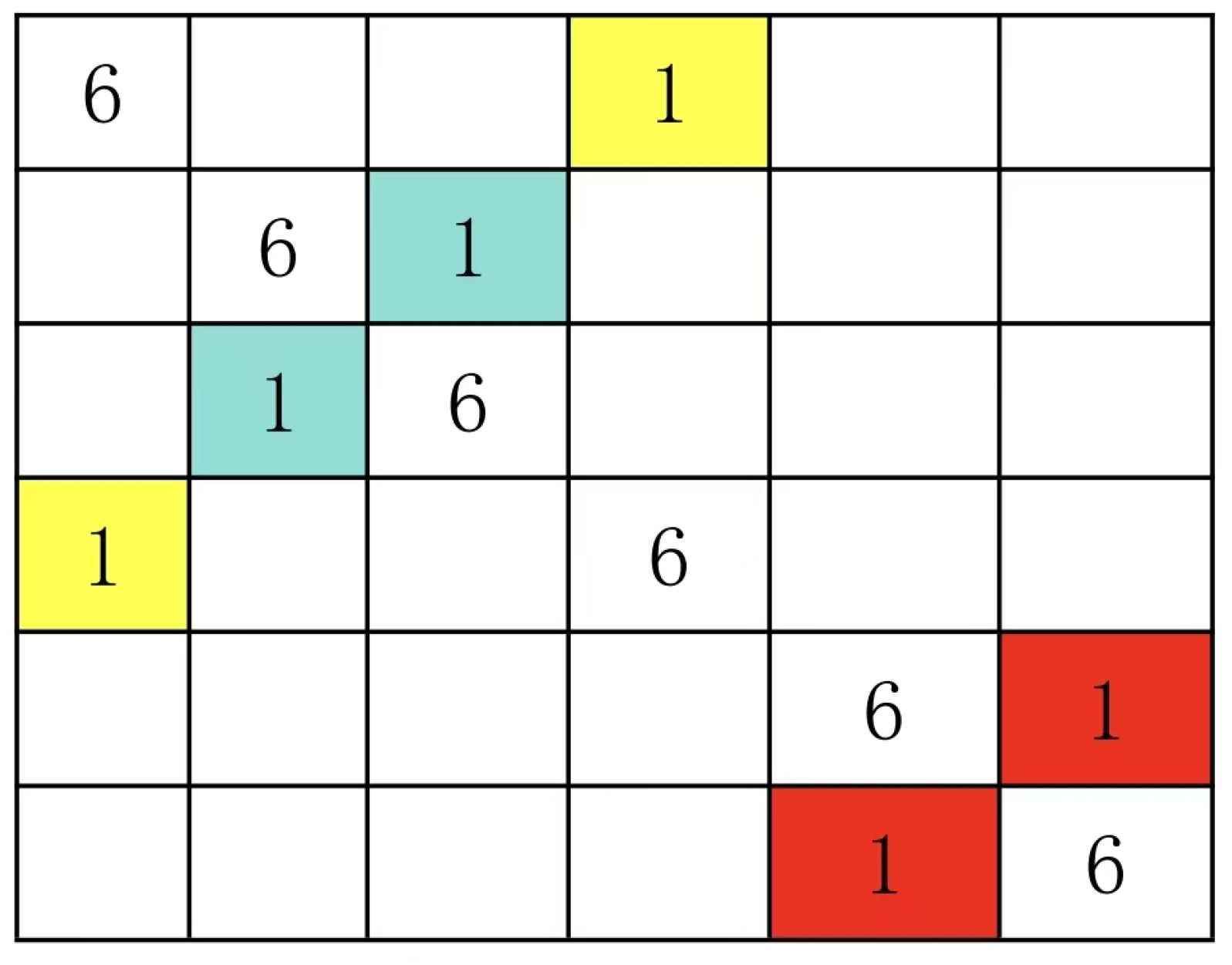
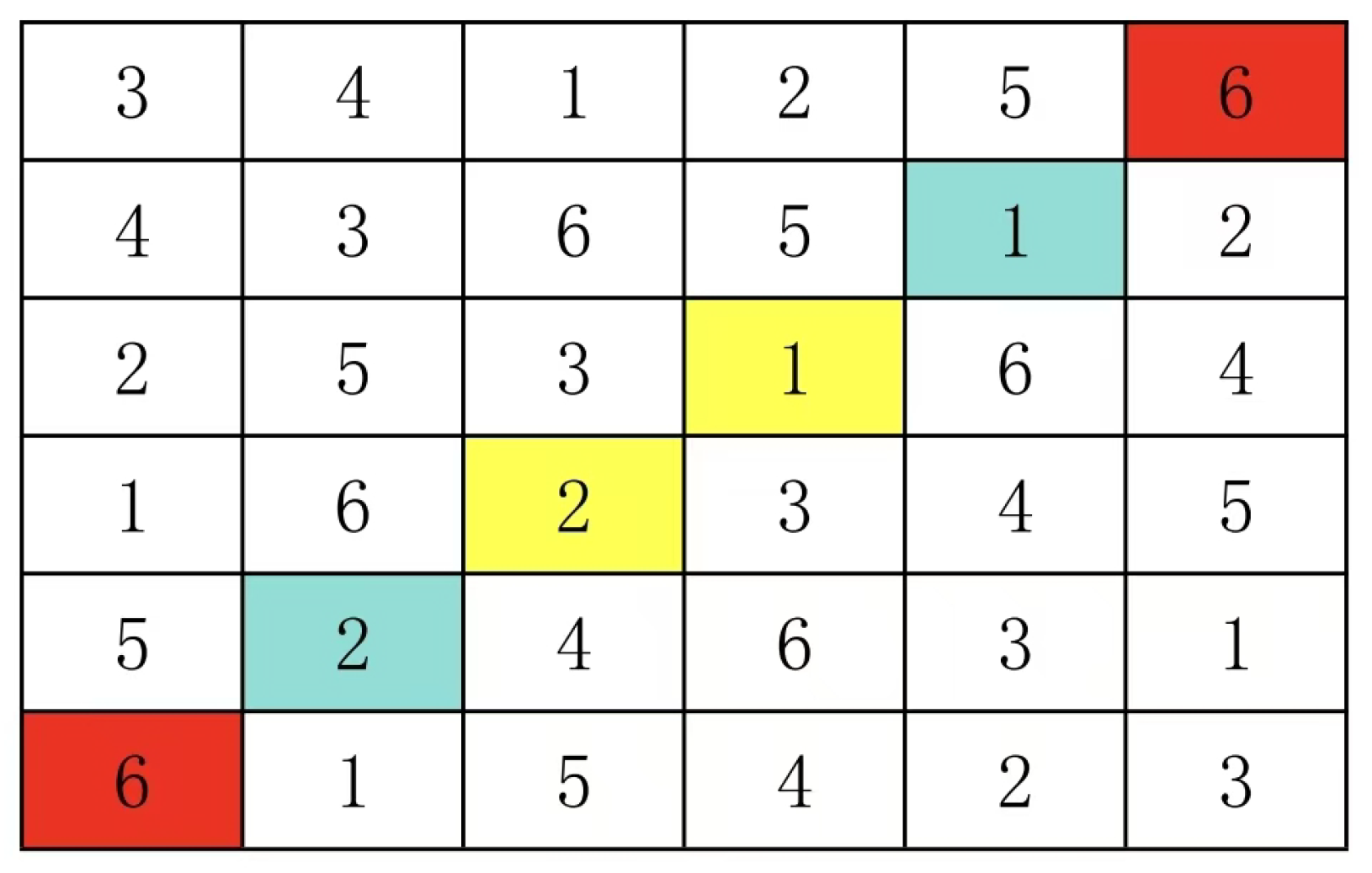
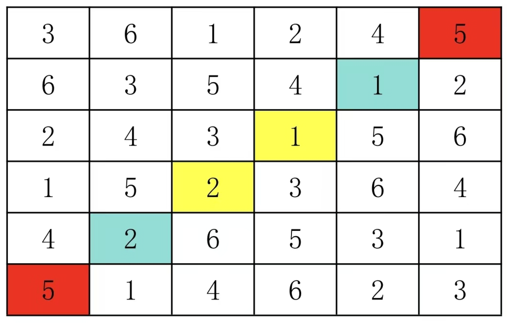
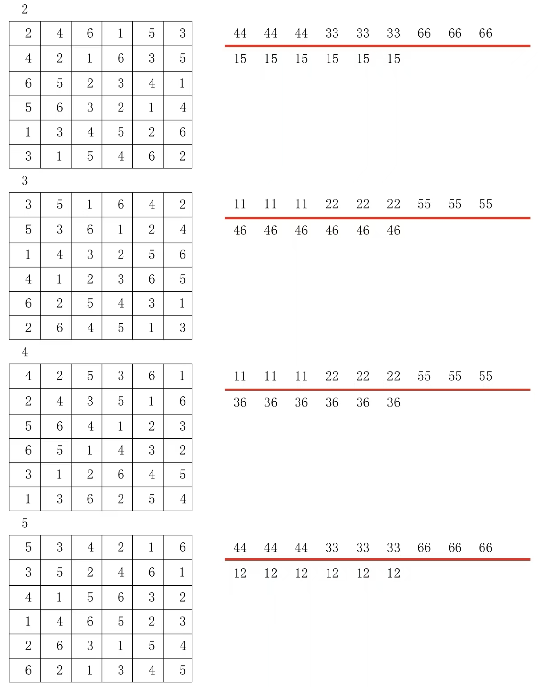
Look at the following 5 by 5 Latin square.

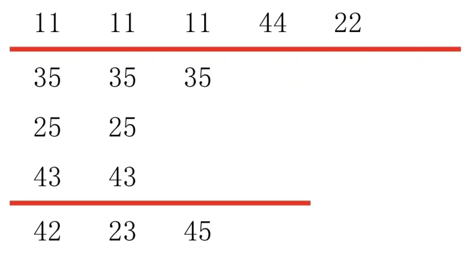
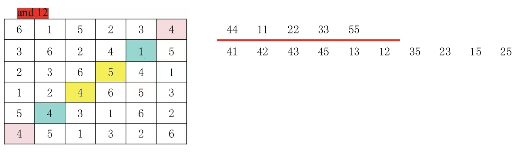
The 5x5 Latin grid pair sets in Figure 2 are (4:4), (4:1), (4:2), (4:3), (1:2), (1:2), (1:3), (1:3), (2:3), and (2:3).

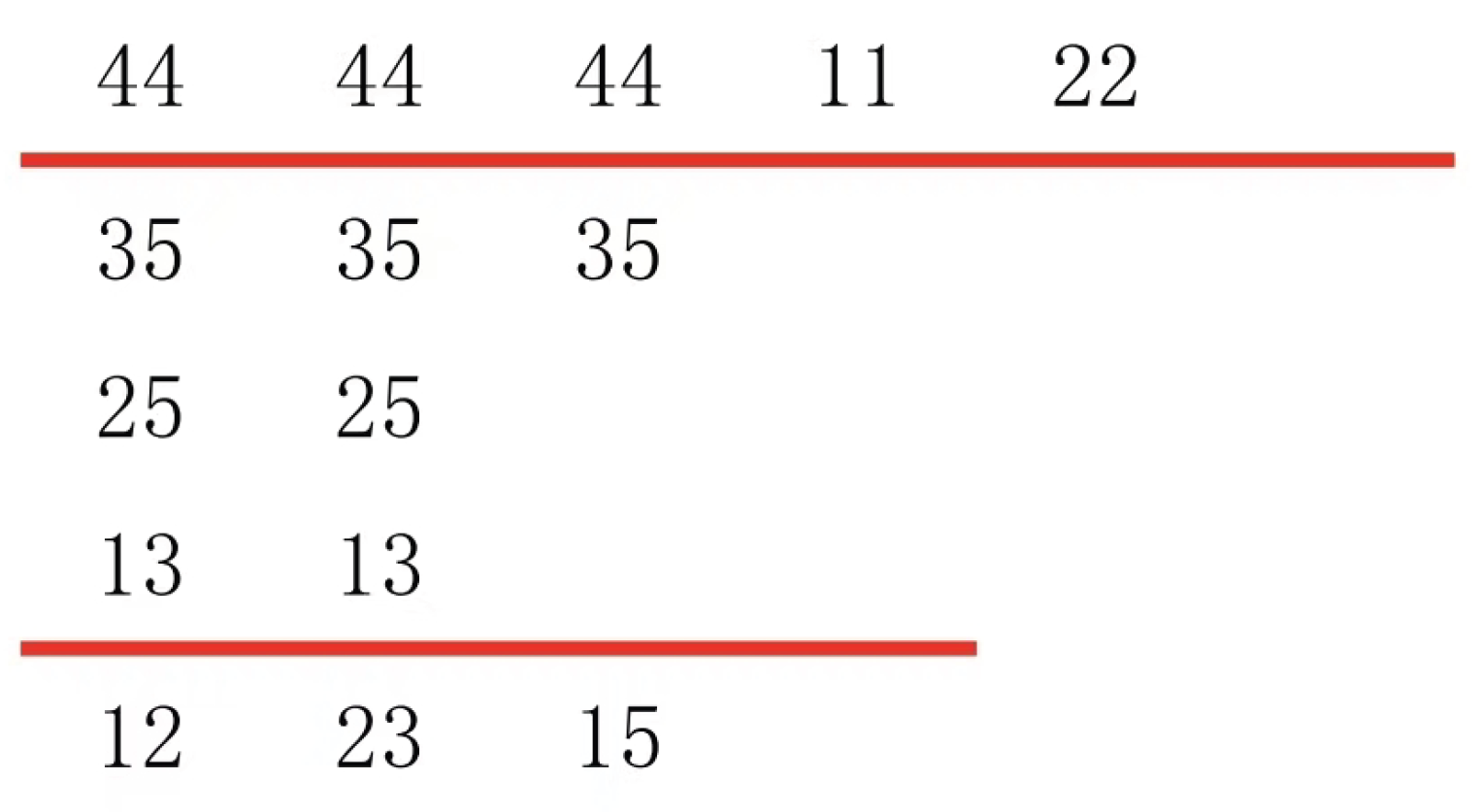
The 5x5 Latin grid pair sets in Figure 1 are (1:4), (1:4), (1:4), (1:4), (1:4), (2:3), (2:3), (2:3), (2:3), and (2:3).

Figure 1 and Figure 2 are different Latin square pair sets. Therefore, the Latin square in Figure 1 cannot be transformed into the Latin square in Figure 2 by row and column replacement.

Figure 1. Graph 1

Figure 1. Graph 1

Figure 2. Graph 2

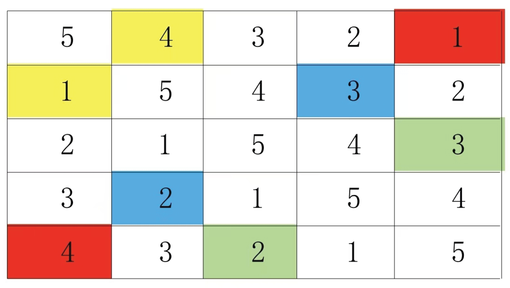
Figure 2. Graph 2

The constraints strictly cover all possible Latin square pairs and ensure non-repetitive permutation of rows and columns in generated configurations. By applying these two constraint rules, we can systematically generate all N× N Latin squares with unique permutation patterns. However, this approach results in an excessively large collection of potential square pairs, making the generation process computationally intensive and inefficient.If multiple cannot form a Latin square, the speed of the generation algorithm will be greatly reduced. Therefore, the following section gives a method to directly obtain the set of pairs that can form a Latin square.

3.2. Generate All N ×N Latin Squares so That the Rows and Columns Do Not Exchange Repeatedly. The Generation Is a Unique Latin Square Algorithm Optimization

All pair groups can be rearranged into the initial region, thus allowing us to derive properties of various pair groups in different regions of the Latin grid or even stronger constraints. When the structure of the initial region pair group is (a: a), the following properties or constraints can be obtained:

• The total number of initial symbols in the structure zone is $N-2$.
• The total number of non-starting symbols in the structure zone is $N-4$.
• Each non-starting symbol in the closing area has four on a 2 by 2 line.
• The number of groups in the structure zone is $(N-3)+(N-4)+\cdots +4+3+2+1$.

If the group structure of the starting region is (a: b), then the following properties or constraints can also be obtained:

1.

The total number of initial symbols in the construct zone is $N-3$.

2.

There are two start symbols in the closing section.

3.

The total number of non-starting symbols in the structure zone is $N-4$.

4.

Each non-starting symbol in the closing area has four positions on a 2-row, 2-column grid.

5.

The number of groups in the structure zone is $(N-3)+(N-4)+\cdots +4+3+2+1$.

Given these properties or constraints, we can generate sets of pairs that could form Latin squares. However, even the minimal set of such pairs generated by this method cannot actually form a Latin square. This problem is clearly an NP problem, though it remains unclear whether it is a NP-complete problem. Interestingly, it appears to be solvable in polynomial time. During my generation process, I observed that if certain pair sets fail to form Latin squares, this becomes evident without requiring exhaustive testing. Through continuous verification, I have confirmed that all 7×7 Latin squares satisfy this condition, though I haven’t yet formally proven it. This conjecture is detailed in the specific steps of the following generation algorithm.

When generating Latin squares, there are two types. The first type contains only pairs with the (a:a) structure within the group set, which exists exclusively in 2N × 2N Latin squares and can be uniquely identified through a very fast generation algorithm to be introduced later. The second type includes Latin squares containing (a:b) pair structures within the group set.

The specific algorithm steps are as follows:

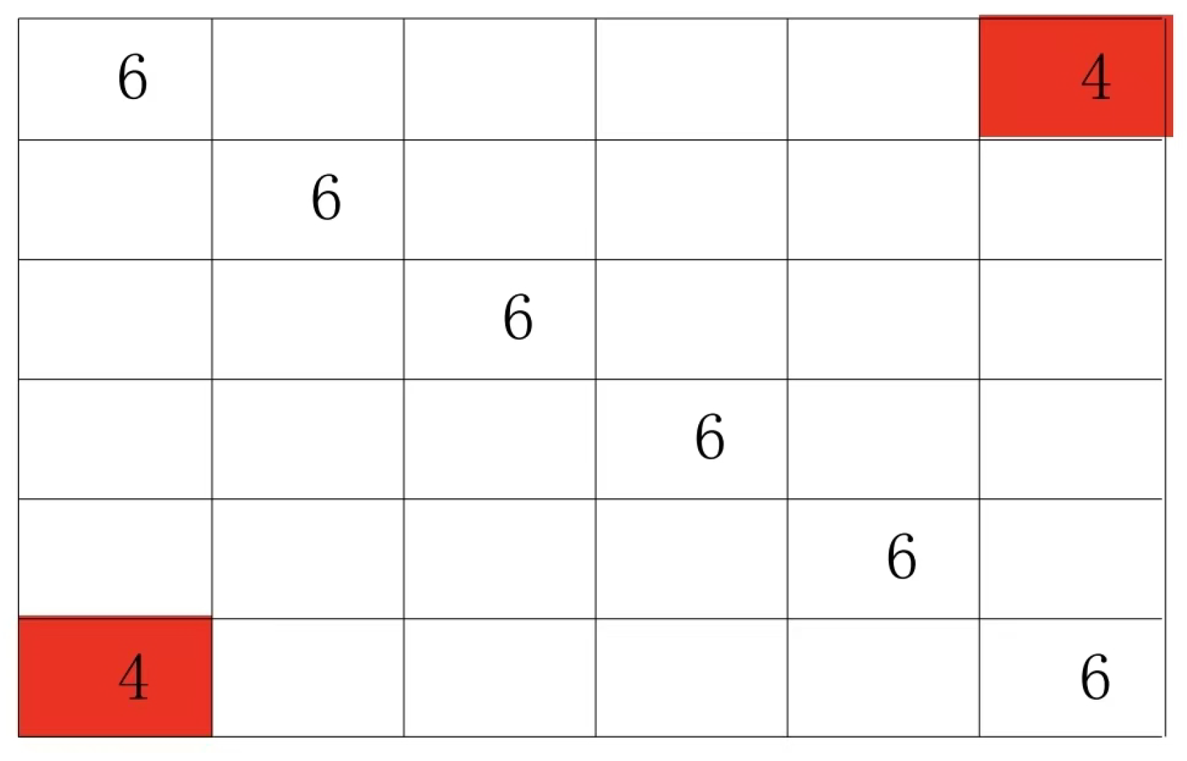
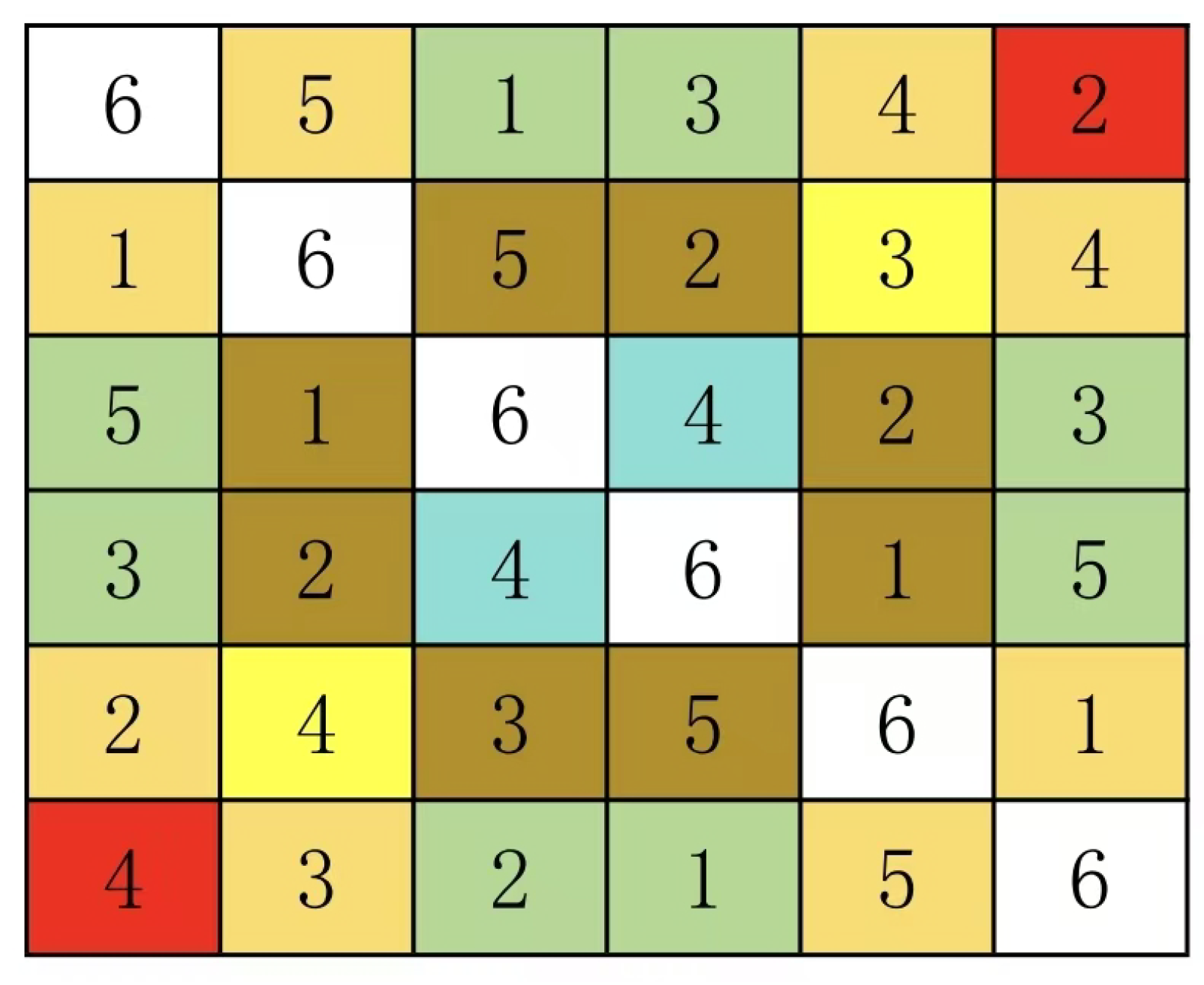
The details are detailed in a 6 by 6 Latin square

1.

Enter the pair group at the starting area (enter (a: a) here to show more details):

Figure 3.

Figure 3.

The set of constraint-conditioned region pairs is (three typical sets are given):

① (4:1) (4:2) (4:3) (4:5) (1:2) (3:5)

② (4:1) (4:2) (4:3) (4:5) (1:3) (2:5)

③ (4:1) (4:2) (4:3) (4:5) (1:5) (2:3)

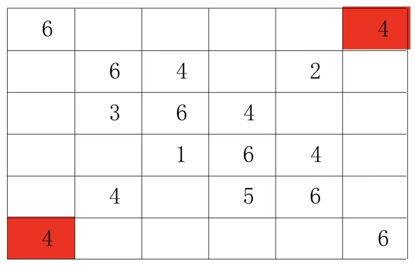
2.

Eliminate the set of groups that satisfy the constraints but do not form a minimal part of the Latin square

Figure 4.

Figure 4.

First, place the pair groups containing start symbols into the construction zone. Interestingly, once these start- symbol pairs are placed, the remaining pair groups can be filled into the construction zone. Once the construction zone is fully populated, the finishing zone will automatically comply with the rules and directly produce a set of pair groups that satisfy the Latin grid requirements. This is my hypothesis as mentioned earlier, which I am currently working to prove.

3.

Construction area group filling techniques

Figure 5. Graph3

Figure 5. Graph3

As shown in Figure 3, the outer group of (4:1) corresponds to (4:2), while groups within the same pair are (4:3) and (4:5). The blue and yellow sections should be filled with (1:2), (3:5), (1:3), (2:5), or (1:5)(2:3). Through trial and error, only (1:2) and (3:5) fit these patterns, while the other pairs violate the rules. The next step involves adjusting relationships between groups: For example, adjust the outer group of (4:1) to (4:5), and the inner pair to (4:2) and (4:3). By systematically testing these combinations, we can complete the construction zone. Latin squares present such inter-group relationships, which remain the biggest challenge in solving their filling algorithm. Although group pairings can be quickly identified, understanding inter-group connections remains an ongoing exploration - this constitutes the primary bottleneck for algorithm speed. While current knowledge lacks clarity about inter-group relationships (e.g., how outer/inner pairings should correspond) or group pairings, efficient filling methods still exist. The core optimization principle allows a group to pair with another either as outer or inner (this generalizes to cases like (a:a) containing symbol a, though this isn’t generalized here). However, when multiple groups combine, their interconnections become fixed. This phenomenon actually reflects a fundamental characteristic of NP-complete problems. In puzzle games, small pieces require complex time complexity to assemble into complete structures. However, when these pieces can be reconstructed using only a few large components, the required combinatorial numbers become significantly fewer. Consequently, certain combinations here essentially have a single solution. The process involves first filling these specific configurations into the construction area, then integrating the remaining elements into the final assembly.

For example, in a 7×7 Latin grid, there are such paired groups (2:2), (3:3), (2:3), (5:5), (6:6), (5:6), (4:4), (4:4), (1:1), and (1:1). Therefore, among the three paired group combinations (2:2), (3:3), and (2:3), only one relationship exists: (2:2) is grouped with (3:3), while (2:3) is grouped with both (2:2) and (3:3). Similarly, the paired group combinations (5:5), (6:6), and (5:6) follow this pattern. As shown in Figure 4, we first fill in the (2:2), (3:3), and (2:3) groups.

Figure 6. Graph4

Figure 6. Graph4

Then fill in (5:5), (6:6), (5:6)

Figure 7. Graph5

Figure 7. Graph5

It can be found that group (5:6) cannot be filled in, because the areas of the outer group corresponding to group (5:5) and (6:6) are exactly the areas of group (2:2). At this time, adjustments are made as shown in Graph 6

Figure 8. Graph6

Figure 8. Graph6

You can actually start by filling in (5:6) and then fill in (5:5) (6:6), which means using the smaller number to lock down the larger one. Fill in the remaining numbers to get

Figure 9.

Figure 9.

Another crucial consideration is to avoid grouping components into external groups whenever possible. While this principle generally holds, exceptions may exist. Each component pair maintains a unique relationship, and there are numerous such combinations. The examples I’ve provided illustrate the algorithm’s operational logic, though it’s unclear whether these pairs are fixed or become less interconnected as more components are added. For instance, the three (1:2) (1:2) (1:2) pairs could form either external or internal groups. However, adding additional (2:2) or (1:2) pairs would reduce their interconnections. While I’ve made some progress in this area, my research remains ongoing and will not be elaborated here.

For this type of pair group set with only one relationship in the construction area, the minimum number increases with N. The minimum number rule is obvious: $2N\times 2N$ and $(2N+1)\times (2N+1)$. The minimum pair group number is N, where $N\ge 3$.

4.

Finally, the finishing area is completed according to the rules

Figure 10. Graph7

Figure 10. Graph7

To complete the Latin grid, I select specific areas in Figure 7 for filling with valid symbols. The blue sections allow numbers 1 and 5, while the yellow sections permit numbers 1 and 2. This creates four possible combinations: 11, 12,51, and 52. Following the established rules, these configurations collectively form the complete Latin grid.

3.3. Algorithm for Generating All N×N Equivalent Class Latin Squares Quickly

Equivalent Latin squares refer to two Latin squares that can be transformed into each other through row permutation, column permutation, or symbol permutation. These two Latin squares are considered isomorphic and belong to the same equivalence class, which some literature also refers to as a homotopy class. Therefore, when generating equivalent Latin squares, it’s crucial to avoid creating new Latin squares that can be transformed into previously generated ones through row permutation, column permutation, or symbol permutation. Since symbol permutation must be avoided, only all distinct pair group structures (specifically the pair group structure of the construction zone) should be generated during the formation of paired groups. Existing structures from previously generated construction zone pairs must be avoided. For example, when generating all 6×6 equivalent Latin squares with a starting zone pair (4:1), the following types of construction zone pair group structures may appear in the 6× 6 Latin square.

① (4:4) (4:1) (1:1) (2:2) (3:3) (5:5) ② (4:4) (4:1) (1:1) (2:3) (2:3) (5:5)

③(4:4) (4:1) (1:1) (2:3) (2:5) (3:5) ④(4:4) (4:2) (1:1) (1:2) (3:3) (5:5)

⑤ (4:4) (4:2) (1:1) (1:2) (3:5) (3:5) ⑥ (4:4) (4:2) (1:1) (1:5) (2:5) (3:3)

⑦ (4:4) (4:2) (1:1) (1:3) (2:5) (3:5) ⑧ (4:4) (4:1) (1:2) (1:2) (3:3) (5:5)

⑨ (4:4) (4:2) (1:3) (1:3) (1:2) (5:5) ⑩ (4:4) (4:1) (1:2) (1:2) (3:5) (3:5)

⑪ (4:4) (4:1) (1:2) (1:3) (2:5) (3:5) ⑫ (4:4) (4:2) (1:2) (1:3) (1:5) (3:5)

⑬ (4:4) (4:2) (1:3) (1:3) (2:5) (1:5) ⑭ (4:2) (4:3) (4:5) (1:2) (1:3) (1:5)

⑮ (4:2) (4:2) (4:3) (1:3) (1:5) (1:5) ⑯ (4:1) (4:1) (4:1) (2:5) (2:5) (3:3)

⑰ (4:1) (4:1) (4:1) (2:2) (5:5) (3:3) ⑱ (4:1) (4:1) (4:1) (2:5) (2:3) (3:5)

⑲ (4:1) (4:1) (1:2) (4:2) (3:5) (3:5) ⑳ (4:1) (4:1) (1:2) (4:2) (3:3) (5:5)

㉑ (4:1) (4:1) (1:2) (4:3) (2:3) (5:5) ㉒ (4:1) (4:1) (1:2) (4:3) (2:5) (3:5)

㉓ (4:1) (1:2) (1:2) (4:3) (4:3) (5:5) ㉔ (4:1) (1:2) (1:3) (4:3) (4:2) (5:5)

㉕ (4:1) (1:2) (1:5) (4:3) (4:3) (2:5) ㉖ (4:1) (1:2) (1:5) (4:3) (4:3) (3:5)

The initial group is (1:1) and the constructed group set structure is

㉗ (5:5) (2:2) (1:1) (1:1) (4:4) (3:3)

There are 27 groups in total. Among them, the first three pairs (1, 2, and 3) containing initial symbols cannot be filled into the construction area. Therefore, these three pairs are excluded. The remaining groups can generate all 6 ×6 equivalent-class Latin squares using the previous algorithm steps. However, some processing is required due to the involvement of the Latin Square Isomorphism Polynomial Algorithm, which I will address later. This section will not continue discussing this treatment as it requires specialized knowledge from the algorithm. After explaining the Latin Square Isomorphism Polynomial Algorithm, the necessary processing techniques will become clear. The algorithm is highly efficient - I manually generated all 22 equivalent-class Latin squares within just a few days.

After obtaining all 6×6 equivalent-class Latin squares, I discovered that generating complete sets of constructive pair group structures wasn’t necessary. Each Latin square inherently contains multiple such group structures. Through processing all 6×6 equivalent-class Latin square transformations, I found only the following 9 groups of constructive pair group structures were required - in fact, fewer might be needed. This led me to focus on just these 9 groups during my analysis.

① (4:4) (1:1) (4:2) (1:5) (2:5) (3:3) ② (4:4) (4:1) (1:2) (1:3) (2:3) (5:5)

③ (4:4) (4:5) (1:3) (1:3) (1:2) (2:5) ④ (4:1) (4:1) (4:1) (2:2) (3:3) (5:5)

⑤ (4:1) (4:1) (4:1) (2:5) (2:5) (3:3) ⑥ (4:1) (4:1) (4:1) (2:3) (2:5) (3:5)

⑦ (4:1) (4:1) (4:3) (1:5) (3:5) (2:2) ⑧ (4:1) (4:2) (4:5) (1:2) (1:5) (3:3)

⑨ (4:1) (4:1) (1:5) (4:3) (2:5) (2:3)

Obviously, it is not necessary to generate all the N × N equivalent class Latin squares by generating all the structures of the pair group set, but it is not clear how to generate the required pair group set, which may be difficult.

3.4. All Main Class Latin Squares Without 2×2 Latin Sub Squares Are Generated Quickly

The main-class Latin grid refers to the extension of equivalence-class Latin grids that allows permutations of three roles: rows, columns, and symbols (for example, a symbol s in row r and column c can be transformed into a symbol r in row c and column s). This transformation is a constant multiple of six. When converting equivalence- class Latin grids to main-class Latin grids, no processing is required. Therefore, the core idea for rapidly generating all main-class Latin grids without 2×2 subgrids is to modify the existing algorithm for generating N×N equivalence-class Latin grids, ensuring the resulting grids contain no 2×2 subgrids. In fact, these 2×2 subgrids specifically refer to the four quadrilateral structures ((a,a)) and ((c,c)), which correspond to the (a:a) pair structure within the group. Thus, the key lies in avoiding such (a:a) pair structures during generation. When constructing the pair structure set, we directly exclude (a:a) pairs to achieve this goal.

Taking the 6×6 Latin grid as an example, the initial pair group is (4:1), and the constructed area pair group structure is

⑭ (4:2) (4:3) (4:5) (1:2) (1:3) (1:5) ⑮ (4:2) (4:2) (4:3) (1:3) (1:5) (1:5)

⑱ (4:1) (4:1) (4:1) (2:5) (2:3) (3:5) ⑲ (4:1) (4:1) (1:2) (4:2) (3:5) (3:5)

㉒ (4:1) (4:1) (1:2) (4:3) (2:5) (3:5) ㉕ (4:1) (1:2) (1:5) (4:3) (4:3) (2:5)

㉖ (4:1) (1:2) (1:5) (4:3) (4:3) (3:5)

The remaining steps are the same as the fast generation of all N × N equivalent class Latin squares and will not be written here.

4. Latin Square Exact Counting Formula Framework

The Latin grid generation algorithm reveals that Latin grids fall into two categories: those containing (a: b) pairs, and those containing only (a: a) pairs. The mathematical description is as follows: Basic definitions and symbols

Consider an N×N Latin square L with a set of numbers S=1,2,...,N. The main line is defined as the diagonal running from the top-left to bottom-right corners (denoted as L(i,i)). The set P consists of binary pairs formed by symmetrically positioned elements along this main line, satisfying the following condition:

The total number of groups is $P={\sum }_{k=1}^{n-1}k={\displaystyle \frac{(N-1)N}{2}}$

Digital total constraint: For any number $a\in S$, the total number of times it appears in all pairs is N

First type of Latin square: (only contains the pair (a: a) groups)

A Latin square L is classified as a non-odd pair Latin square (Category I) if all pairs in it are composed of identical symbols, meaning for any pair $(x,y)\in P$, we have $x=y$. In this case, the pair can be represented as $\{(a,a)\mid a\in S^{\prime }\}$ where $S^{\prime }\subseteq S\setminus \left\{\mathrm{main}\mathrm{line}\mathrm{numbers}\right\}$. Each number a corresponds to a pair that appears exactly N times in total.

Type II Latin grid: (contains pairs of (a: b))

In the set of paired groups within an $N\times N$ Latin square, consider the paired group T. If there exist two distinct numbers y and z ($y\ne z$) such that $\forall e\in T$, $e=y$ or $e=z$, and y and z ... A pair group is classified as the second type when its occurrence count satisfies the constraint on the total number of digits within the group (where all digits in each pair group sum to N), while T also fulfills the constraint on the total number of pairs $(N-1)+(N-2)+\cdots +2+1$. The second type of pair groups represents typical pair group structures.

Latin square exact count = type 1 Latin square + Type 2 Latin square

First class Latin grid generation algorithm

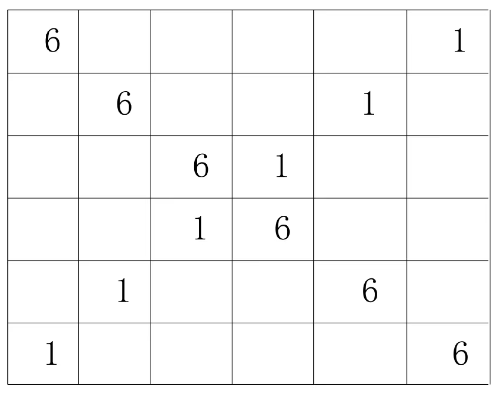
As can be seen from the definition of the first type of Latin square group, this type of Latin square group is very clear and can know all the outer groups of the square group, so there is a very efficient generation algorithm. Take the 6×6 Latin square with 6 as the main line as an example

6 × 6 Latin squares satisfying the first category of pairs are (1:1) (1:1) (1:1) (2:2) (2:2) (2:2) (3:3) (3:3) (3:3) (4:4) (4:4) (4:4) (5:5) (5:5) (5:5)

The outer group of (1:1) is (1:1) as follows

Figure 11.

Figure 11.

(1:1) (1:1) (1:1) are equivalent to other pair groups. Therefore, by swapping rows and columns, we avoid the already existing pair group positions in the diagram. Subsequent pairs also avoid previously existing pair group positions. The row-column swapping operation that avoids positions in the diagram is one of

Figure 12.

Figure 12.

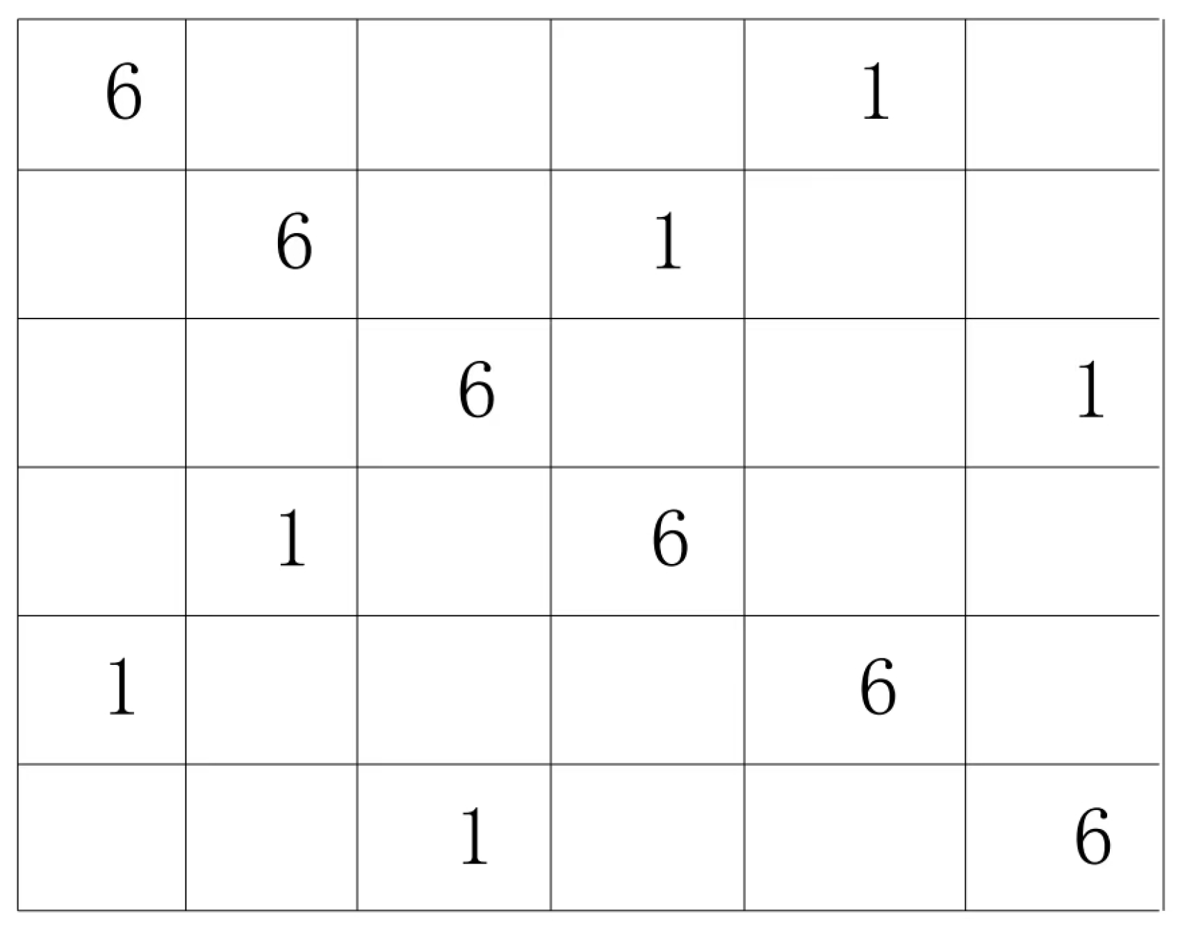
Instead of the previous two row swaps between groups that already exist

Figure 13.

Figure 13.

[H]

Instead of the previous three row-to-column swaps that already exist

Avoid the first four existing row-to-column swaps as

Figure 14.

Figure 14.

Figure 15.

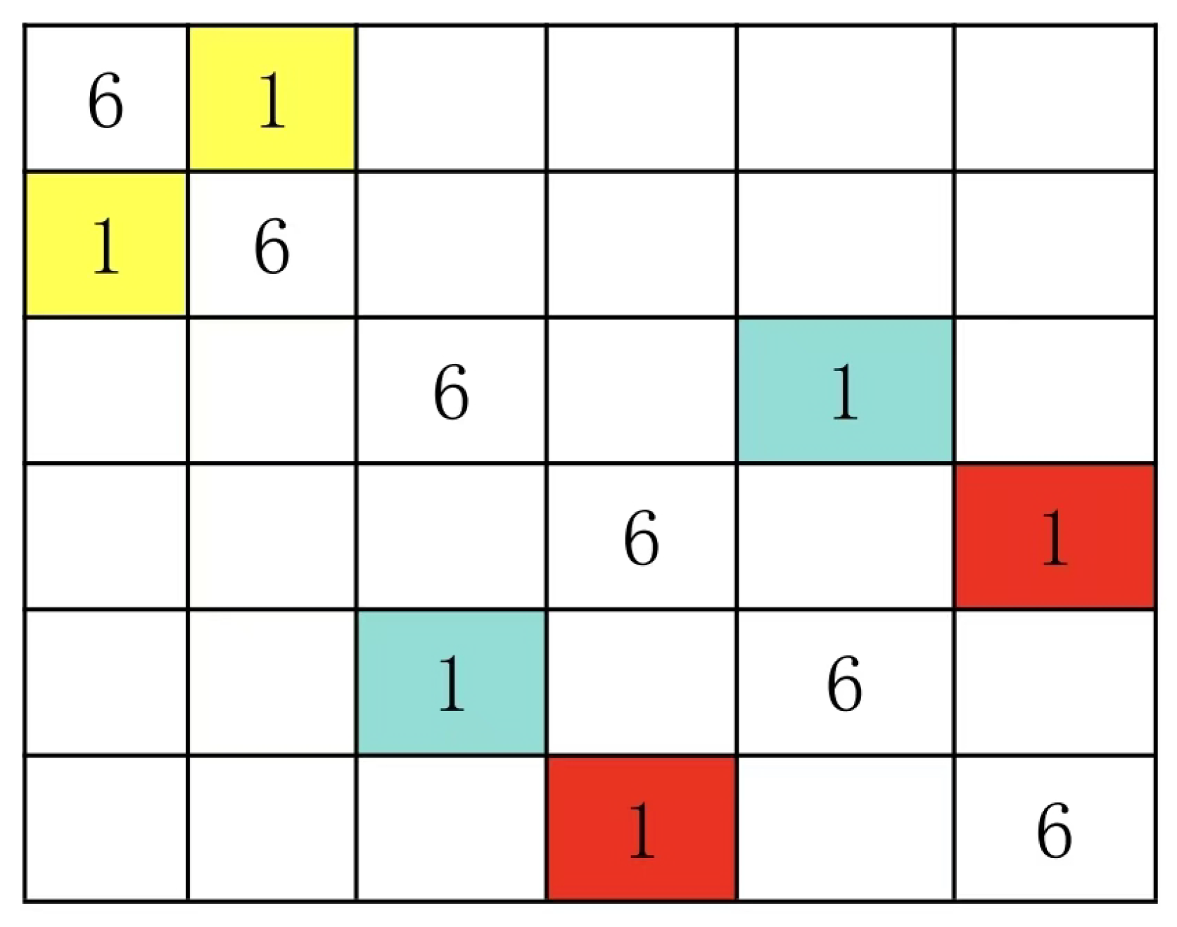
Figure 15.

By replacing the first five positions with 1, 2, 3, 4, and 5 respectively, it is easy to obtain this type of Latin square for pairs. The 6x6 Latin square that satisfies the first type of pairs is

Figure 16.

Figure 16.

As long as we know the group, the outer group can be used to quickly generate the Latin square with the above algorithm, so the key to the generation algorithm and the solution algorithm is to solve the relationship between the group.

The first type of Latin square exists only in a 2N by 2N space, and there is only one.

The second type of Latin square generation algorithm

The second category of Latin squares can be classified as containing complete sets of pairs. For instance, in a 5×5 Latin square centered around 5, all possible pair combinations (essentially every possible pairing of two symbols) are 12, 13,41,23,42, and 43. A 5×5 Latin square with a pair set containing (4:4), (4:2), (4:1), (4:3), (1:2), (1:2), (1:3), (1:3), (2:3), and (2:3) exemplifies this complete set, as every possible pairing exists within it. Another scenario involves partial pair sets. Consider a 5×5 Latin square with pairs (1:4), (1:4), (1:4), (1:4), (1:4), (2:3), (2:3), (2:3), (2:3), and (2:3). While it lacks the complete pair set (1:2), (1:3), (4:2), and (4:3), it still contains at least one type II pair set.

The mathematical description is

Full combination type II Latin square:

If the permutation pair set $P^{\prime }\subseteq P$ of type II Latin squares L contains all possible numerical combinations in set C (i. e., for any $(x,y)\in C$, there exists at least one permutation pair $(x,y)$ or $(y,x)$), then L is termed a full permutation type II Latin square. In this case, the permutation pair set satisfies $C\subseteq \{(x,y)\mid (x,y)\in P^{\prime }\mathrm{or}(y,x)\in P^{\prime }\}$. Example: When $N=5$ and the main line number is 5, $C=\left\{\right(1,2),(1,3),(1,4),(2,3),(2,4),(3,4\left)\right\}$. If the permutation pair set contains all six combinations mentioned above (allowing repetitions), it belongs to the full permutation category.

Some combinations are in the second category: Latin squares:

If the odd pair group set $P^{\prime }$ of the second type Latin square L only contains some digital combinations in C (that is, there are $(x,y)\in C$ such that both $(x,y)$ and $(y,x)$ are not in P), but at least contains one odd pair group, it is called the second type Latin square of partial combination L.

Example: When N=5, a Latin square pair group consists of five groups (1,4) and five groups (2,3), which only contain two combinations in C, belonging to the partial combination class. The rigor of classification is shown

Exclusivity: The first and second types of Latin squares have no intersection, because the former group is the same number, the latter contains at least one odd group; in the second type, all combinations and partial combinations are also exclusive, because the former contains all combinations, the latter only contains part.

Completeness: Any N × N Latin square belongs to either category 1 or category 2 (completely combined or partially combined).

Equivalence and Derivation Basis: Since permutations (x, y) and (y, x) are structurally equivalent under matrix permutation swaps (as evidenced by interchangeable row-column exchanges), these pairs can be treated as identical combinations when formulating counting formulas, thereby simplifying combinatorial analysis of set C. This classification establishes a structured theoretical framework for precise counting algorithms. By processing combination counts across distinct scenarios through recursive or divide-and-conquer approaches, we ultimately derive the total number of Latin squares.

The counting method I’ve adopted above is intuitive and easy to understand, but its practical derivation isn’t ideal. This is mainly because some combinations in the second type of Latin squares require full transformations into the second type. Additionally, groups with identical Latin square structures might actually be two completely different Latin squares (which seems solvable here). I also considered directly counting equivalent Latin square groups, but faced similar challenges due to varying group structure configurations when using different symbol layouts as main lines. Another difficulty lies in constructing group structures that can not form Latin squares. During formula derivation, I kept exploring whether these non-formatted group structures actually represent a category and their potential connections. This led me to propose my conjecture, which shifted my research direction. My initial focus was solving precise counting for arbitrary N×N Latin squares. These are the difficulties and approaches I encountered, hoping they’ll help you. Although no particularly useful formulas have been written yet (as they’re not fully accurate), you could adopt alternative methods. The generation algorithm I provided earlier allows for other classification approaches for counting.

5. Algorithm for Latin Square Isomorphic Polynomial

Two Latin squares are isomorphic if they can be transformed into each other through row permutation, column permutation, or sign permutation. To determine their isomorphism in polynomial time, four theorems are required. These theorems are derived from the definitions of Latin squares, group properties, outer group properties, and homogroup properties.

Theorem 1: If all the pairs of Latin squares in two Latin squares are the same in group or outer group, then the set of pairs of Latin squares must be the same.

Theorem 2: Pairings that are mutually external can be transformed to sub-axes by row-column swapping in polynomial time.

Theorem 3: Two Latin squares are identical under subline transformations in the main line canonical form if they can be mutually transformed through row and column permutations without symbolic substitution. This means these Latin squares can be identified as mutual pairs for subline operations within polynomial time, thereby making them completely identical.

Theorem 4: In a Latin square, if swapping positions of symbols a and b results in positions c and d also being swapped, then the swap of symbols a and b is equivalent to swapping symbols c and d. This means that after swapping symbols a and b, symbols c and d are also swapped. Therefore, the Latin square remains unchanged, as swapping symbols a and b again swaps both c and d. Note that multiple swaps may be equivalent because swapping positions of symbols a and b sometimes involves more than one pair of symbols. As long as positions are swapped, their symbol swaps are considered equivalent. Theorem 3 can be easily derived from Theorem 1 and Theorem 2, while Theorem 3 provides a simple proof and Theorem 4 offers a concrete interpretation.

Give a 9 by 9 Latin square and a 6 by 6 Latin square to illustrate

Figure 17.

Figure 17.

Any permutation of the (4:6) group on the initial region transforms the group into the light red area in the diagram. The outer group of any (4:6) group(5:3) The row-column permutation is transformed to the secondary main line in blue in the figure. At this time, the same group of group (4:6) and group (5:3) is shown in the cyan part of Figure 8.

Figure 18. Graph8

Figure 18. Graph8

Figure 19. Graph9

Figure 19. Graph9

The paired group (3:1) is the outer group of the paired group (4:6) and the paired group (5:3). The paired group (3:1) and the paired group (4:6) are shown in the light orange section of Figure 9. The paired group (3:1) and the paired group The same group (5:3) is shown in the brown part of Figure 9, so as above, the outer group also corresponds to the corresponding position.

Figure 20. Graph10

Figure 20. Graph10

Figure 21. Graph11

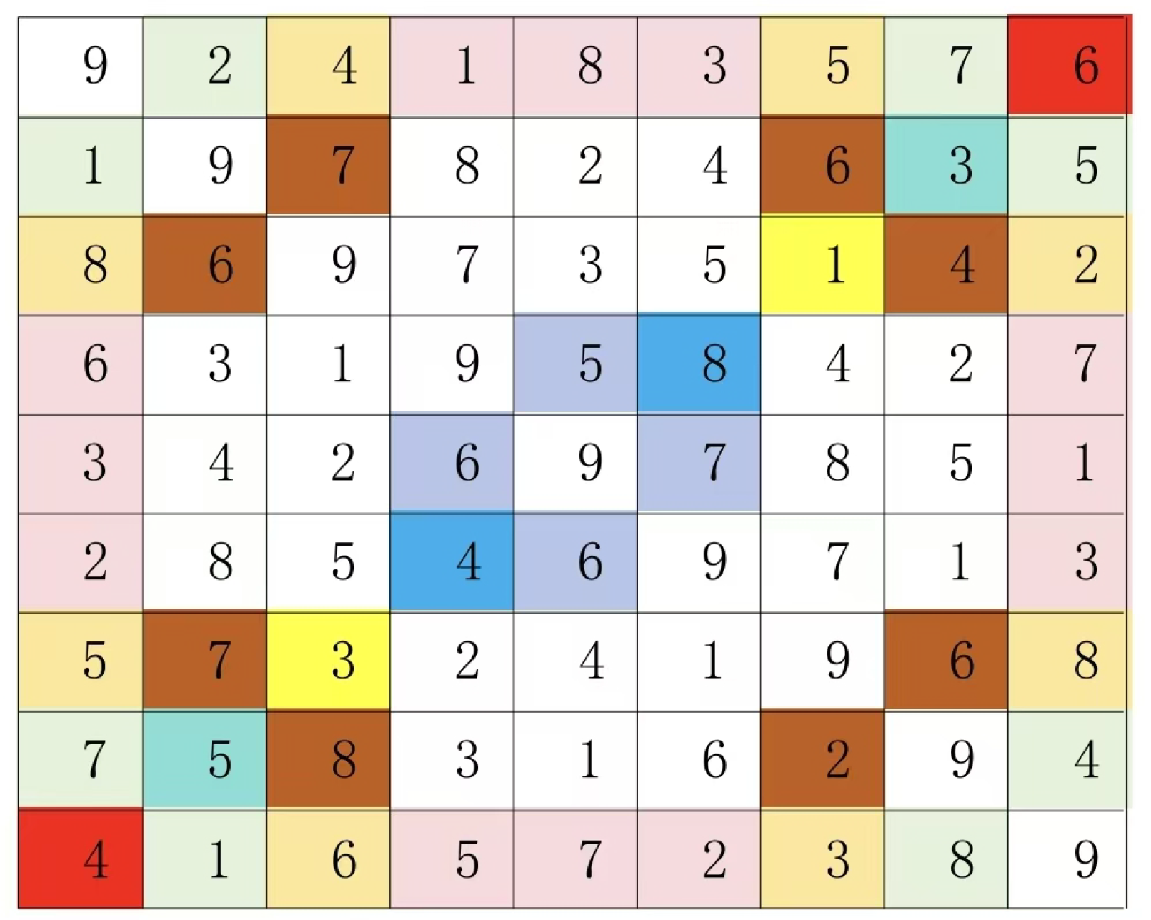
Figure 21. Graph11

When paired groups on the secondary mainline are mutually external, their corresponding positions remain fixed. However, in odd-order Latin squares, there exists a portion that does not correspond to either the blue or light blue sections shown in Figure 10. This specific area can be uniquely identified by any single paired group within it.

The following is a specific explanation of Theorem 4 using the 6×6 Latin square as an example

Figure 22. Graph12

Figure 22. Graph12

The Latin square in Figure 13 is obtained by swapping the positions of group (1:2) in Figure 12

Figure 23. Graph13

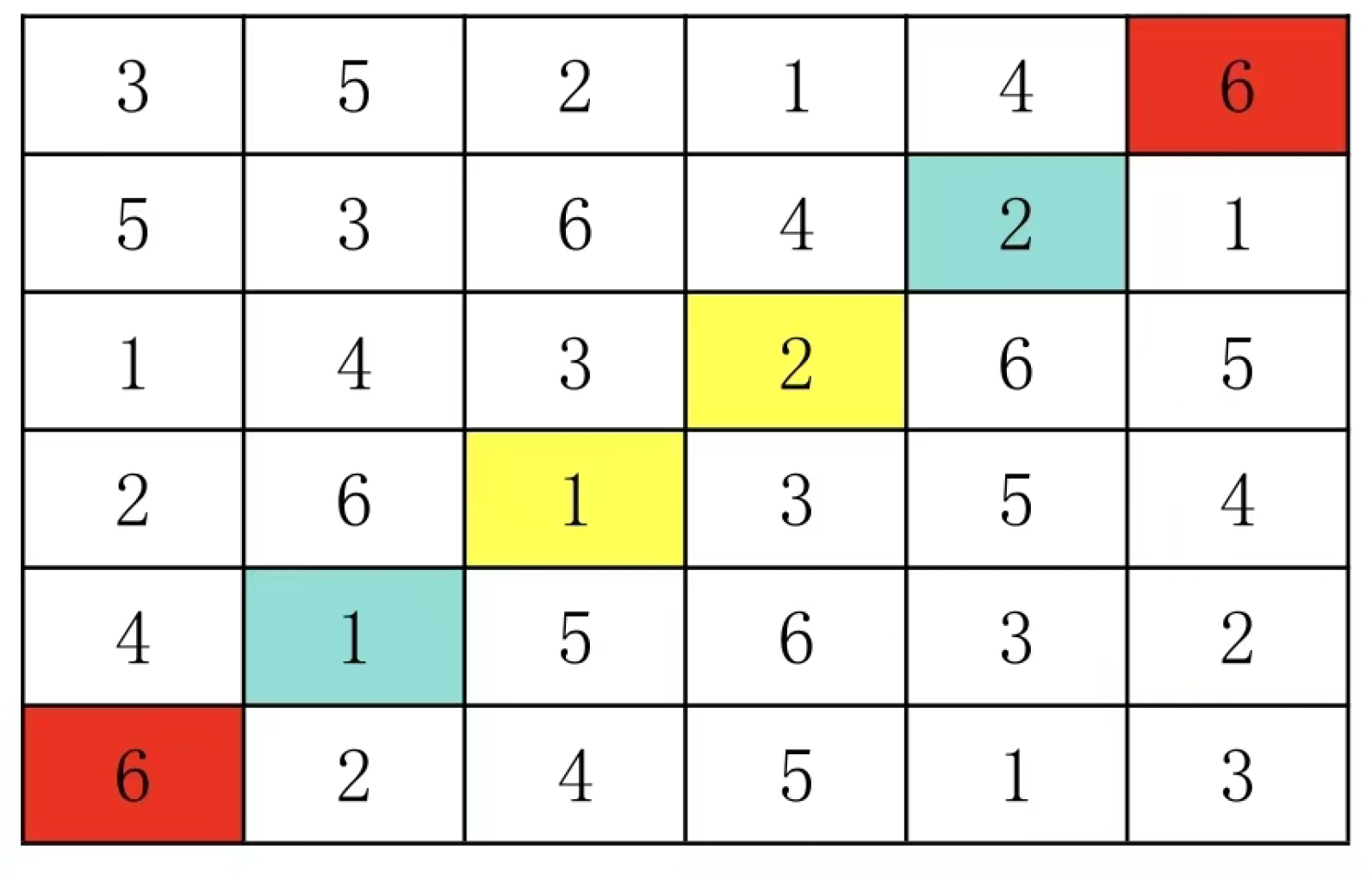
Figure 23. Graph13

It can be observed that after the positions of numbers 1 and 2 are swapped, the positions of numbers 4 and 5 also swap. In fact, not only do numbers 4 and 5 swap positions, but numbers 5 and 6 also swap positions, as shown in Figure 14.

Figure 24. Graph14

Figure 24. Graph14

Now I’m going to use the 6 by 6 Latin square to show you how to do the Latin square isomorphic polynomial algorithm

1. First, compare the group structure of all numbers (symbols) as the main line. Look at the 4 A Latin grid and the 18A Latin grid.The group structure of numbers (symbols) as the main line in the 4A Latin grid is

Figure 25.

Figure 25.

Figure 26.

Figure 26.

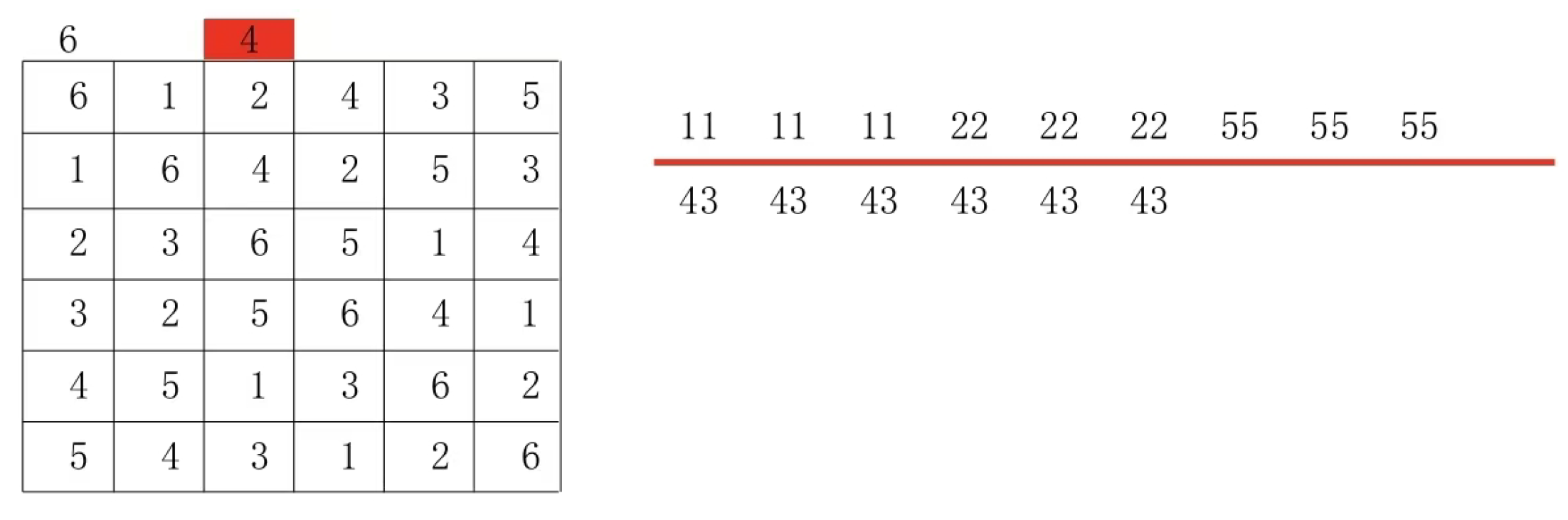
Figure 27.

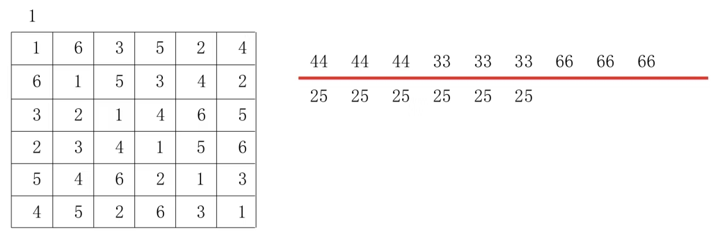
Figure 27.

18A Latin square numbers (symbols) as the main line group structure are respectively

Figure 28.

Figure 28.

Figure 29.

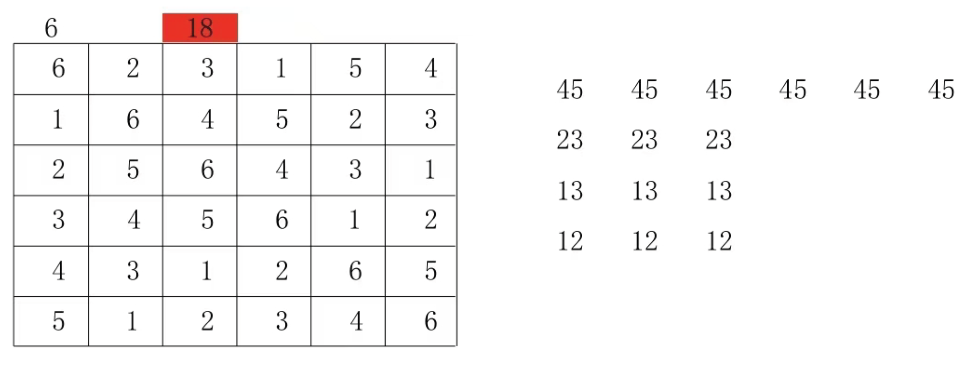
Figure 29.

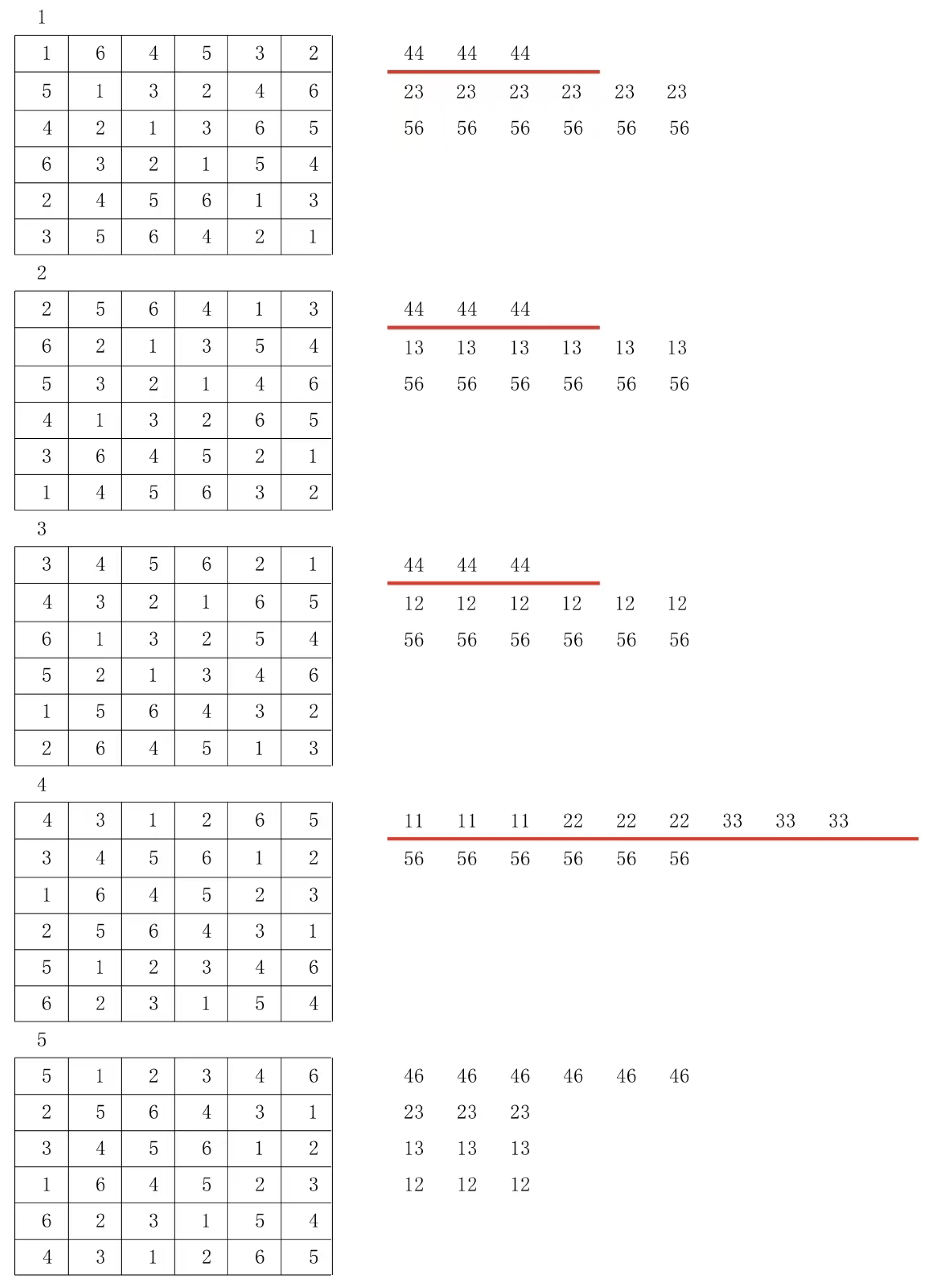
It can be immediately observed that the group structure of 4A Latin Grid using all numbers as main lines differs entirely from that of 18A Latin Grid. This directly proves that 4A and 18A Latin Grids are not isomorphic, with a time complexity of $2n^3$, as the differing group structures cannot be resolved through numerical substitution. The group structure of 4A Latin Grid using all symbols as main lines remains identical. Such Latin Grids may possess unexpected algebraic properties due to their exquisite symmetry, which I will further investigate in subsequent studies.

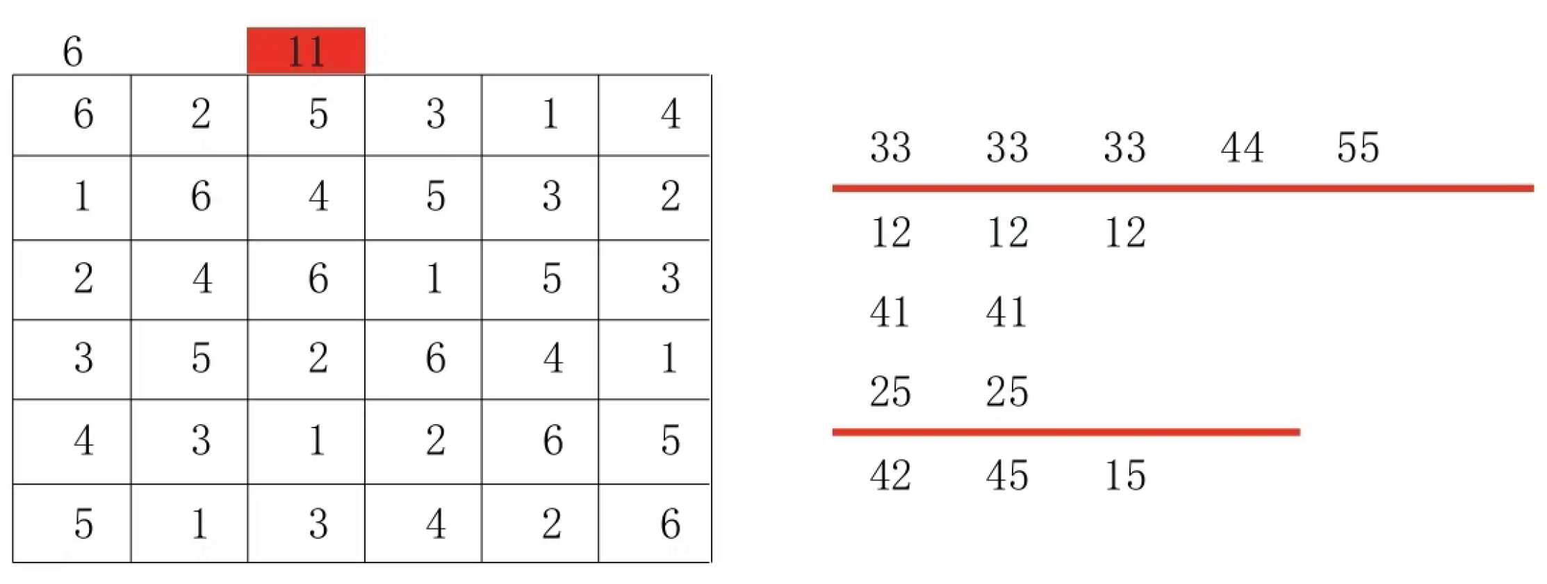
2.The Latin grid structure with all symbols forms the same main line grouping structure such as the 9A Latin grid and the 11A Latin grid. The 9A Latin grid maintains identical main line grouping structures for all numbers.

Figure 30.

Figure 30.

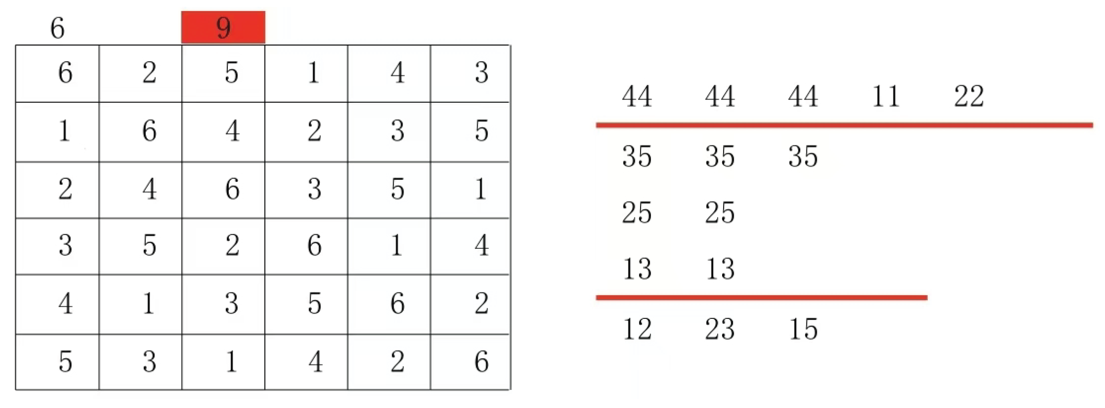
11A The Latin grid has all the numbers as the main line and the group structure is also the same

Figure 31.

Figure 31.

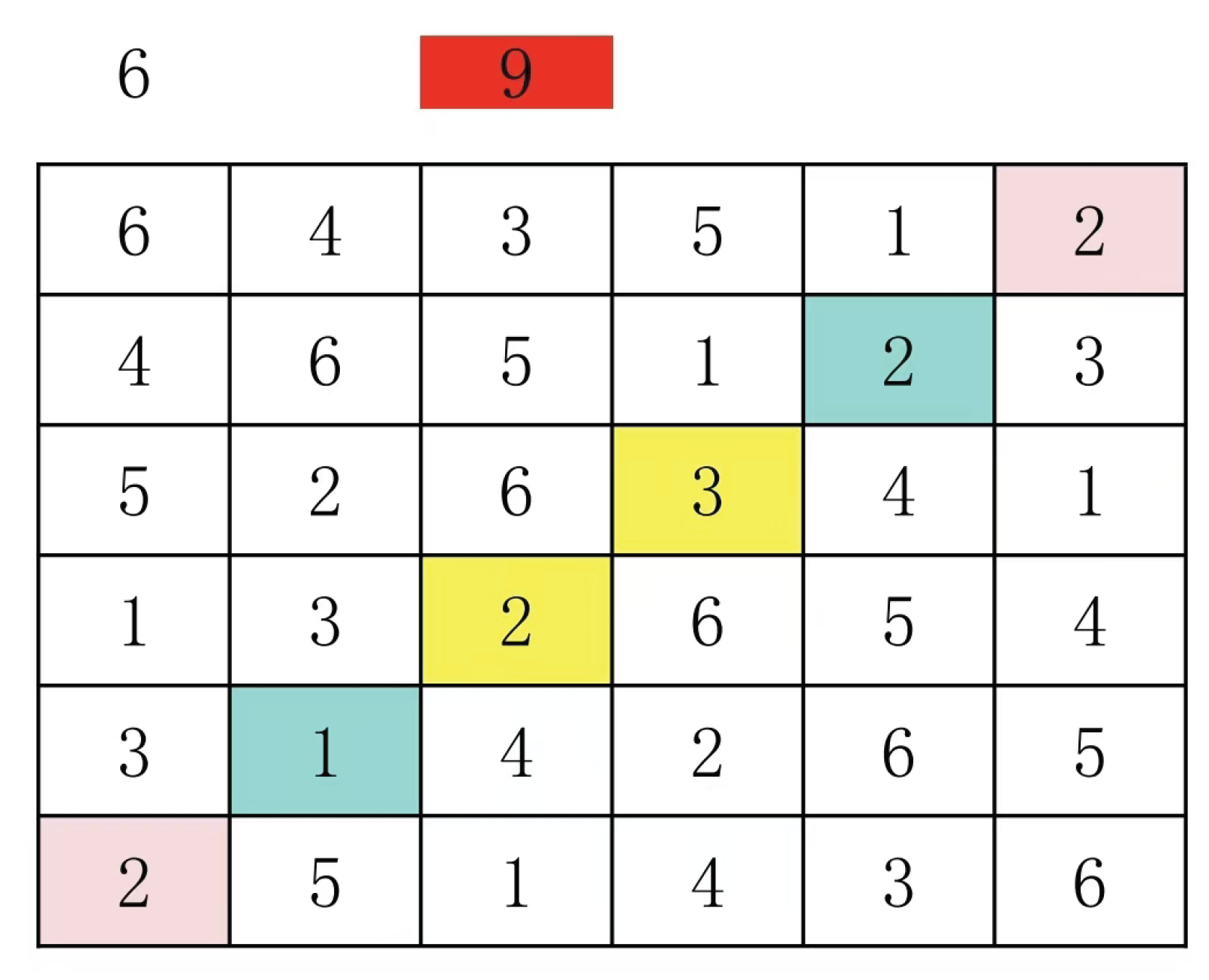
Next, align the 9A Latin Grid with the 11A Latin Grid by matching their paired sets, then select identical outer groups for the secondary mainline. In the 11A Latin Grid: swap positions 4 and 3, then swap positions 3 and 1 (note that this is the swapped version of 3), followed by swapping positions 2 and 5. This alignment ensures the 9A and 11A Latin Grids share identical paired sets.

9A Latin square

Figure 32.

Figure 32.

11A Latin square

Figure 33.

Figure 33.

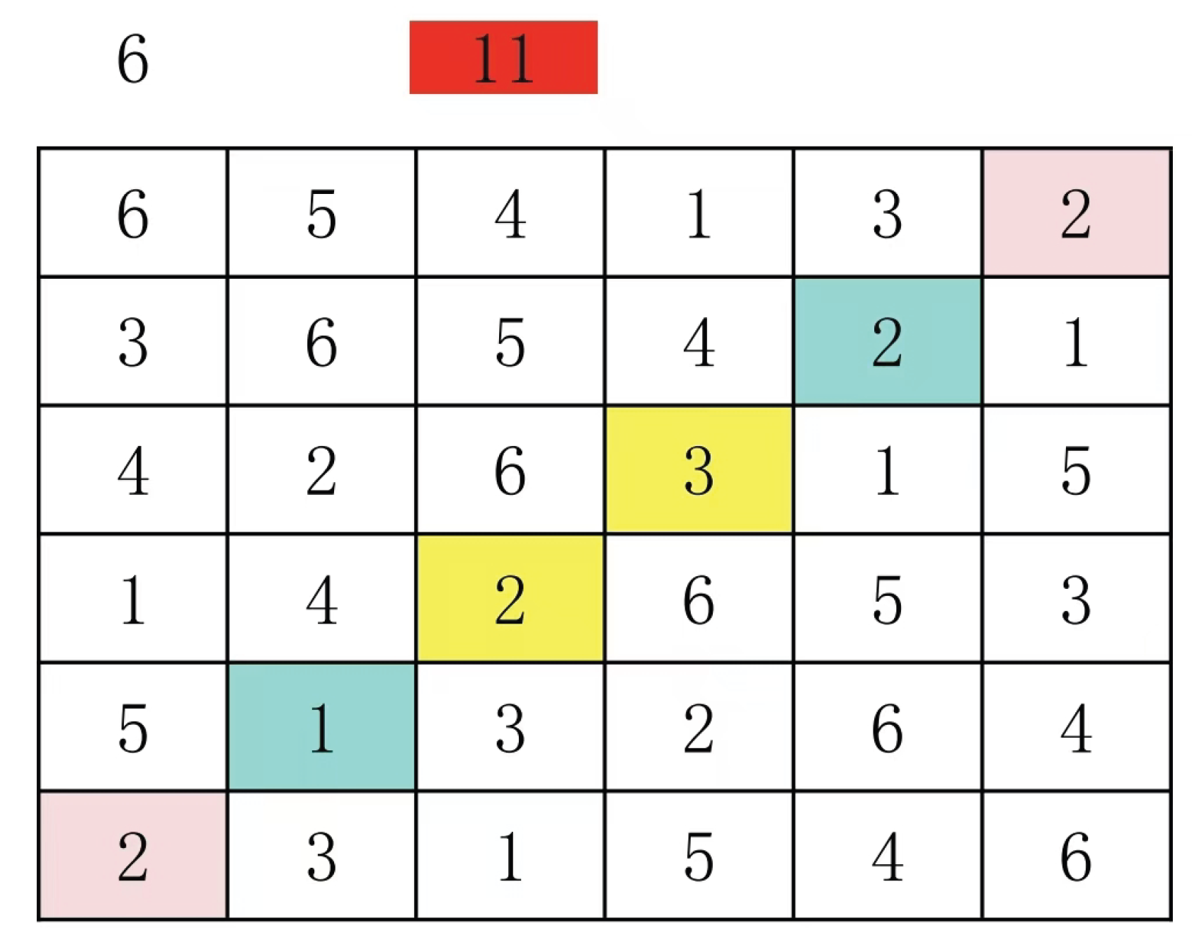
It has been observed that all pair groups in these two Latin squares exhibit symmetry about the secondary axis. Let me propose a hypothesis: If the primary axis group structure of all symbols in both Latin squares is identical, then their pair groups would also be symmetrical about the secondary axis. However, for configurations like 9A and 11 A Latin squares, such symmetry through the secondary axis would result in mirror images. While my digitally transformed version of 9A maintains the same primary axis group structure, its pair groups are not symmetric about the secondary axis. This phenomenon holds true for other Latin squares. The symmetry’s inherent beauty compels me to persistently seek proof, with potential complete documentation of this hypothesis in future versions. Subsequent testing will verify whether digital transformations alter the pair group structures.

The set of pairs is

Figure 34.

Figure 34.

For example, 4 and 1 are replaced to get

Figure 35.

Figure 35.

The structure of the group set remains unchanged as long as the main line configuration stays consistent. Therefore, the 9A and 11A Latin squares cannot undergo numerical substitution. As the number of rows increases, the proportion of these Latin squares grows significantly. My random sampling tests on 9×9 Latin squares consistently revealed this pattern, which is evident in their group set structures. Numerical substitution does alter the group structure, and according to Theorem 3, 9A and 11A Latin squares are not isomorphic. However, some configurations can be transformed through row-column permutations, provided no numerical substitution occurs. Theorem 3 remains applicable in such cases.

3.All symbols in the two Latin squares are grouped together with the same main line structure, and the group structure of the number replacement group is also unchanged. For example, 6A Latin square and 12A Latin square

Figure 36.

Figure 36.

Figure 37.

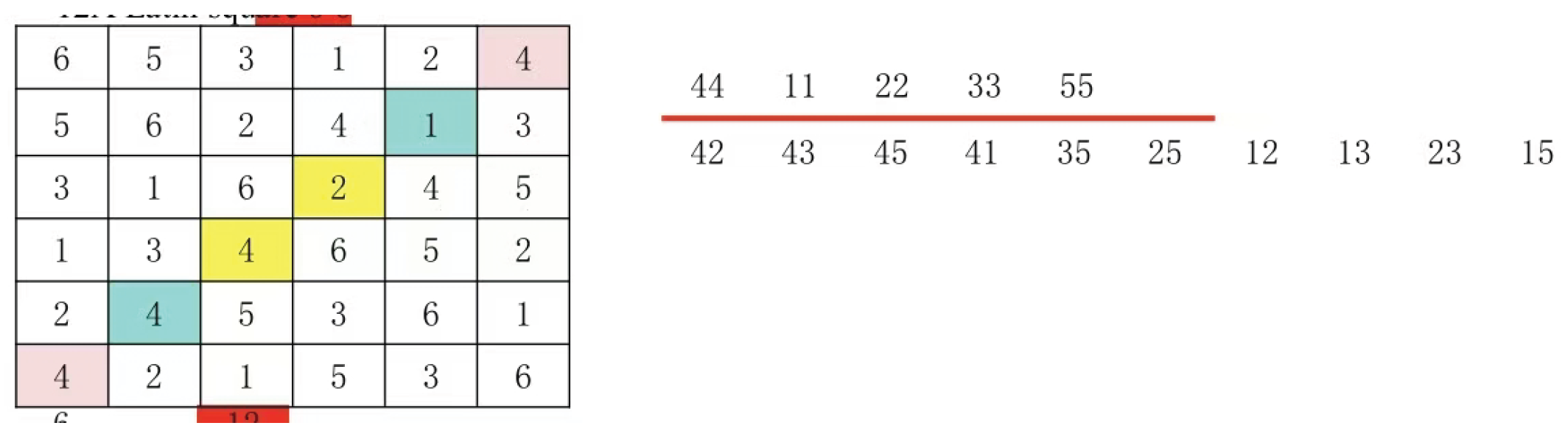
Figure 37.

Through numerical substitution analysis, we observed that swapping numbers between 4 and 1, 4 and 2, 4 and 3, 4 and 5, 1 and 2, 1 and 3, 1 and 5, 2 and 3, 2 and 5, and 3 and 5 does not alter the group composition. However, this substitution modifies the relationships between outer groups and within groups. When the symbolic relationships between outer and within groups are aligned, they become isomorphic if the secondary main lines match; otherwise, they are not.

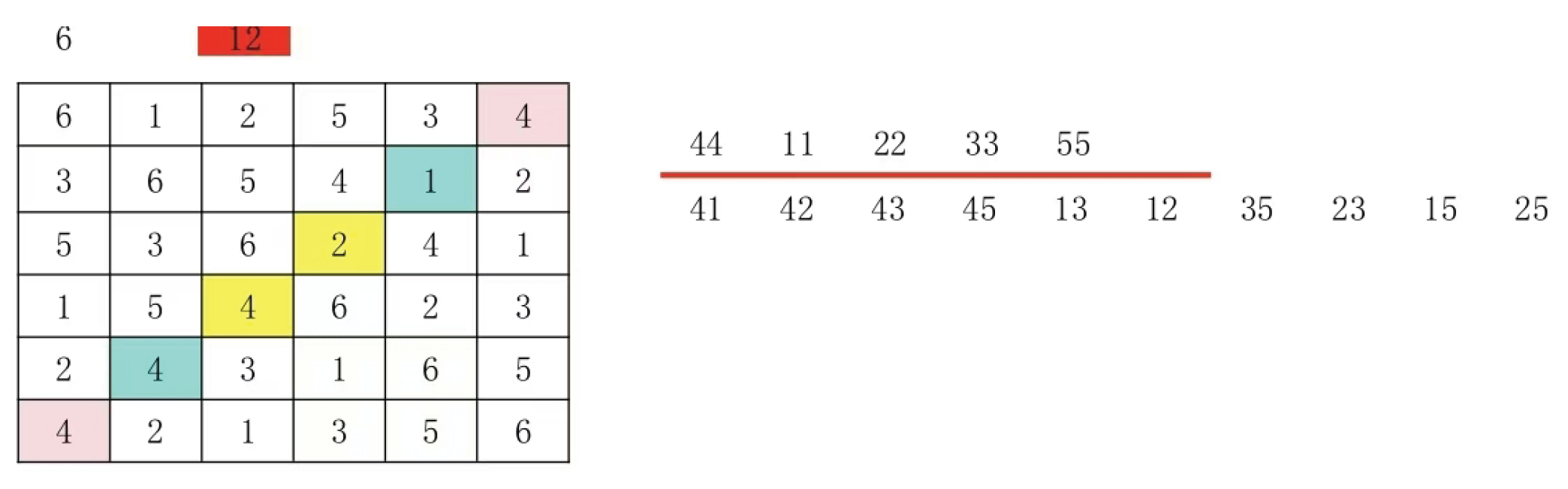
For example,2 and 5 replace

Figure 38.

Figure 38.

At this point, the same group of pair groups (4:1) becomes a pair group (4:2), or you can compare all the outer groups and all the same groups of the pair groups by sorting them out. The relationship between the outer groups and the same groups of all the pair groups can be made the same through symbolic replacement in polynomial time, which is also an operation in polynomial time.

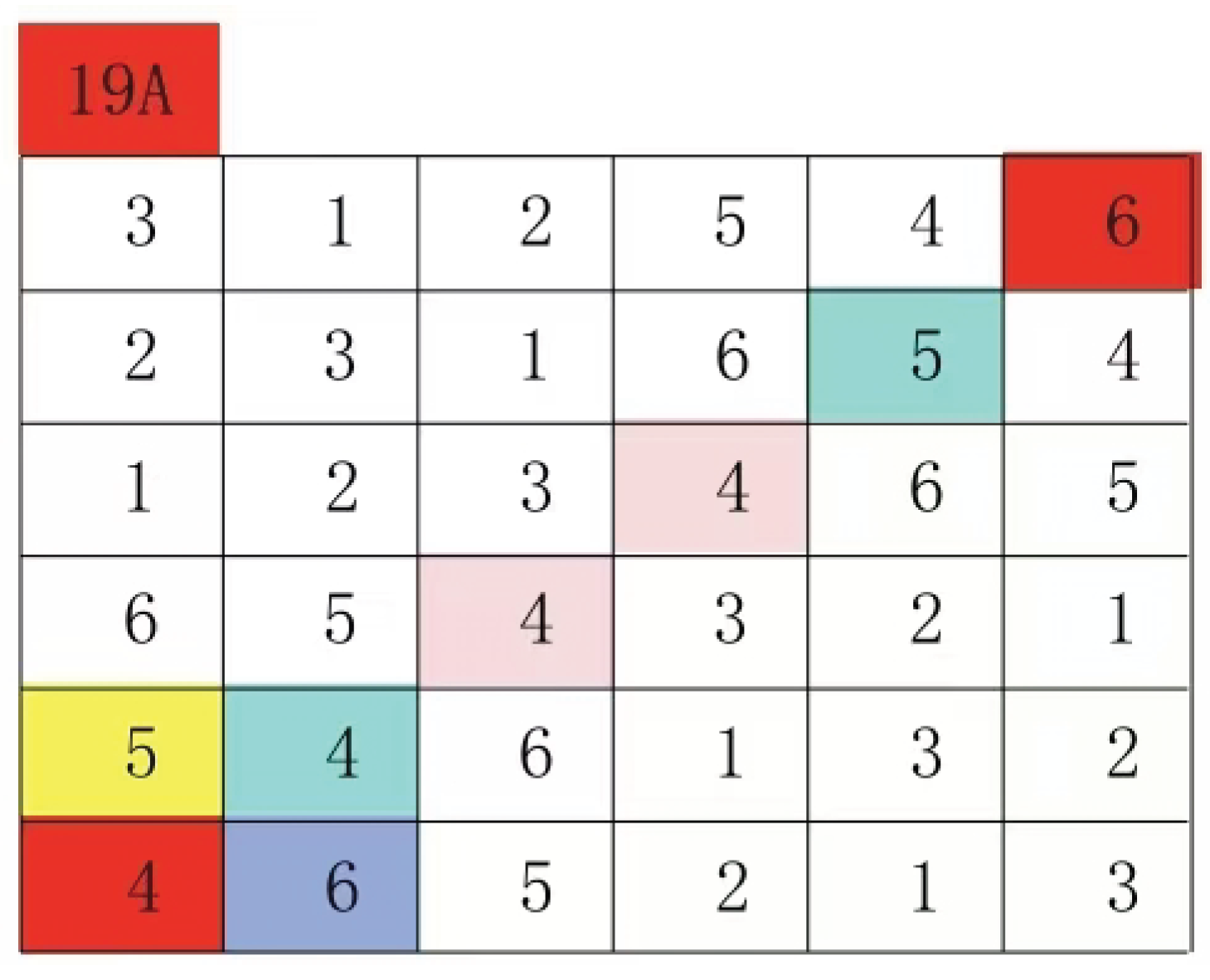
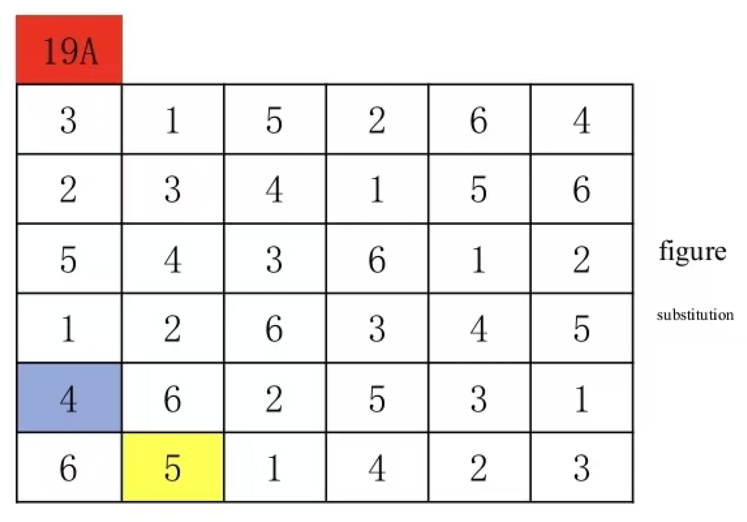
4.Both Latin squares share identical group structures for their main line operations. The group structure remains unchanged under number permutation, and neither external nor internal group relationships between them are altered. According to Theorem 3, we can determine whether two Latin squares are isomorphic within polynomial time by examining sub-line transformations that exclude number permutation operations. For instance, when comparing Latin square 19A and 22A, it’s crucial to avoid applying sub-line transformations during number permutation processes.

Figure 39.

Figure 39.

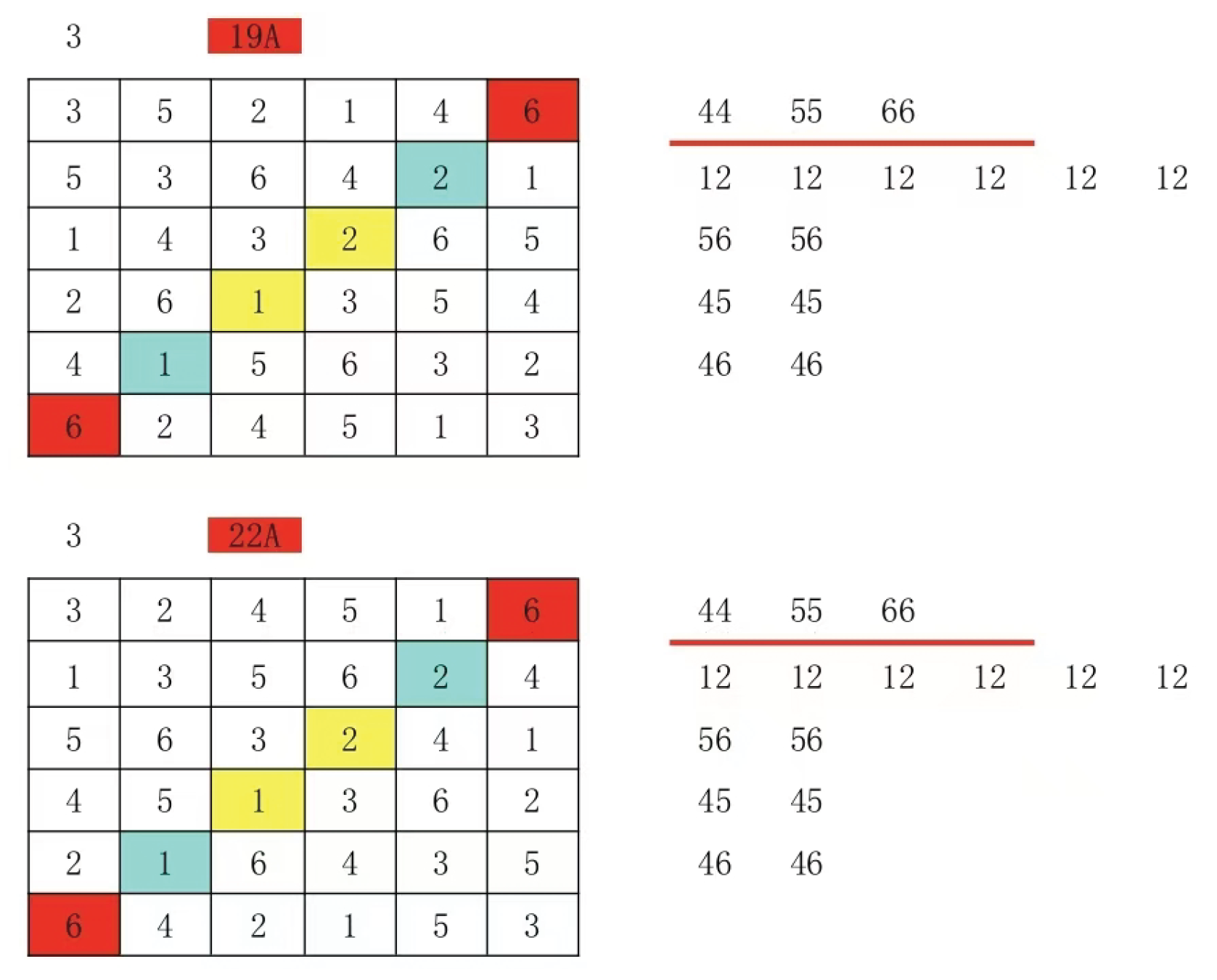
The secondary mainline does not contain the numbers 4 and 5 in the group. Therefore, these two numbers are swapped to check if they can be rearranged. If not, it indicates that these two Latin squares are not isomorphic. Note that in this step, only number combinations are excluded, meaning the total number of combinations is (n²-n)/ 2.

If the secondary line in the group contains numbers to be replaced, it may transition to the primary line. However, the secondary line pair in the Latin grid must consist of replacement numbers, meaning each secondary line should contain exactly one number to be replaced. The secondary lines must not contain two replacement numbers simultaneously. For example, 10A Latin grid.

Figure 40.

Figure 40.

Figure 41.

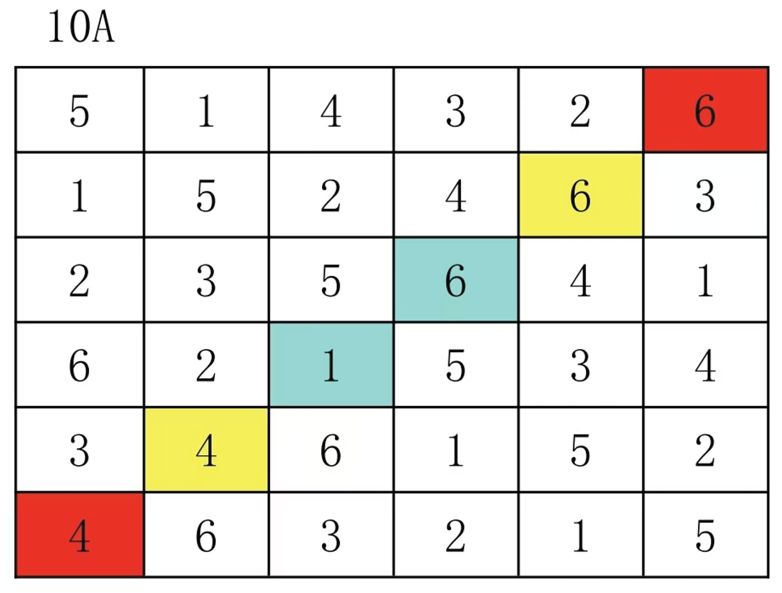
Figure 41.

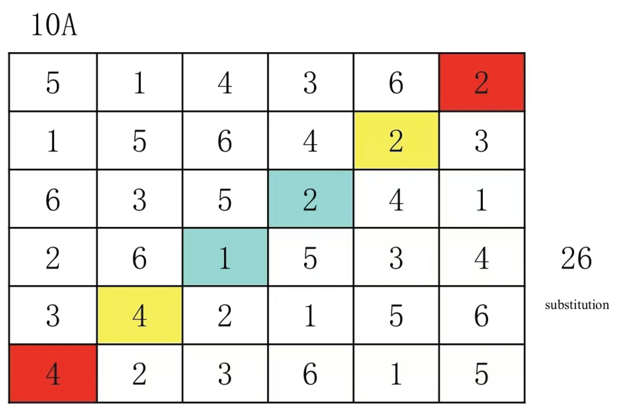
At this stage, I have tested that even 6×6 Latin squares can be processed in polynomial time. However, since there’ s no guarantee that sub-rows will follow the aforementioned patterns, nor can we ensure that all two-number permutation tests will complete without being mapped to another, these two Latin squares remain isomorphic. As I haven’t provided proof of this, it might already be possible to solve Latin square isomorphism within polynomial time at this point. Nevertheless, I didn’t stop there and instead presented a polynomial-time algorithm for Latin square isomorphism that resolves all the aforementioned scenarios.

5.To solve the Latin Grid isomorphism problem in polynomial time, Theorem III serves as the cornerstone. While the secondary mainline structure of Latin Grid numbers undergoes transformation after digit replacement, its underlying modulo form remains unchanged. The key lies in identifying the corresponding secondary mainline modulo form within polynomial time. In the 19A Latin Grid framework, any digit replacement initially preserves its modulo form structure. This preservation mechanism is crucial for understanding the secondary mainline modulo form’s behavior.

Figure 42. Graph15

Figure 42. Graph15

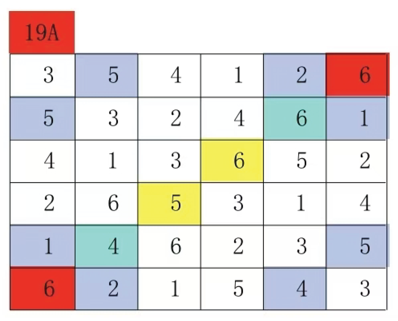
Make a secondary main line for any group, then swap the numbers 6 and 5

Figure 43. Graph16

Figure 43. Graph16

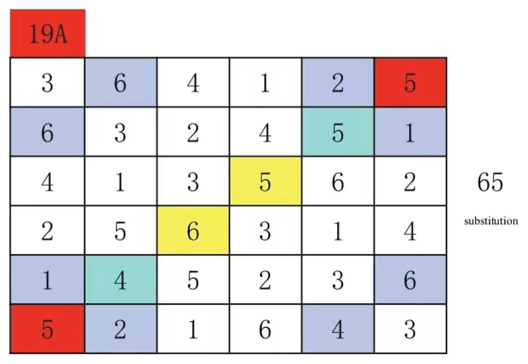
As deduced from Theorem 3, the submainline modulo form remains invariant. In Figures 15 and 16, the steel-blue sections represent positions of group (6:6) and group (4:6) within their respective groups, as well as positions of group (5:5) and group (4:5) within their respective groups. Each steel-blue section position corresponds one-to-one with its corresponding permutation in both groups. Similarly, positions of group pairs on the submainline also maintain this one-to-one correspondence. Therefore, directly searching for the submainline modulo form enables solving Latin grid isomorphism problems within polynomial time. Below we detail the algorithmic steps using the 19A Latin grid as an illustration.

Figure 44. Graph17

Figure 44. Graph17

Figure 45. Graph18

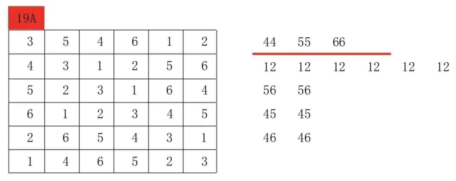
Figure 45. Graph18

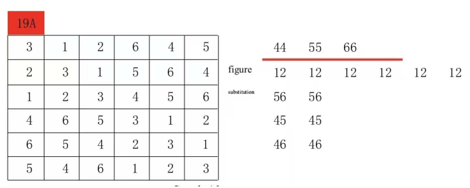
Figure 18 After digital replacement of the Latin grid, the submainline group selection in Figure 17 is (4:6), (4:5), and (4:4). Generally, the submainline group containing more identical numbers is selected, but it can also be randomly selected without affecting the result. However, this selection is convenient for processing and more intuitive

Figure 46. Graph19

Figure 46. Graph19

Next, select any replaceable number (the previously mentioned number substitution does not alter the group set) for corresponding purposes. Of course, structural correspondence is also required. Group (1:2) cannot correspond to Group (5:6) because these two groups have different quantities. Here, I choose numbers 4 and 6 to correspond. Therefore, the red pair group (4:6) in Figure 19 corresponds to the pair group (6:4), and the blue pair group (4:5) in Figure 19 corresponds to the pair group (6:5)

Figure 47. Graph20

Figure 47. Graph20

It is evident that the secondary mainline patterns in Figure 19 and Figure 20 differ significantly. Specifically, the yellow number 5 in Figure 20 should correspond to the steel-blue position, while the steel-blue number 4 should occupy the yellow position. Furthermore, the same group positions in Group (4:6) and Group (4:5) of Figure 19 are paired as (2:1) (1:2), whereas in Figure 20, the corresponding group positions of Group (6:4) and (6:5) are (2:1) (2:1). If the secondary mainline patterns were identical, the number 2 would correspond to the number 1. Therefore, we must switch the positions accordingly.

Figure 48. Graph21

Figure 48. Graph21

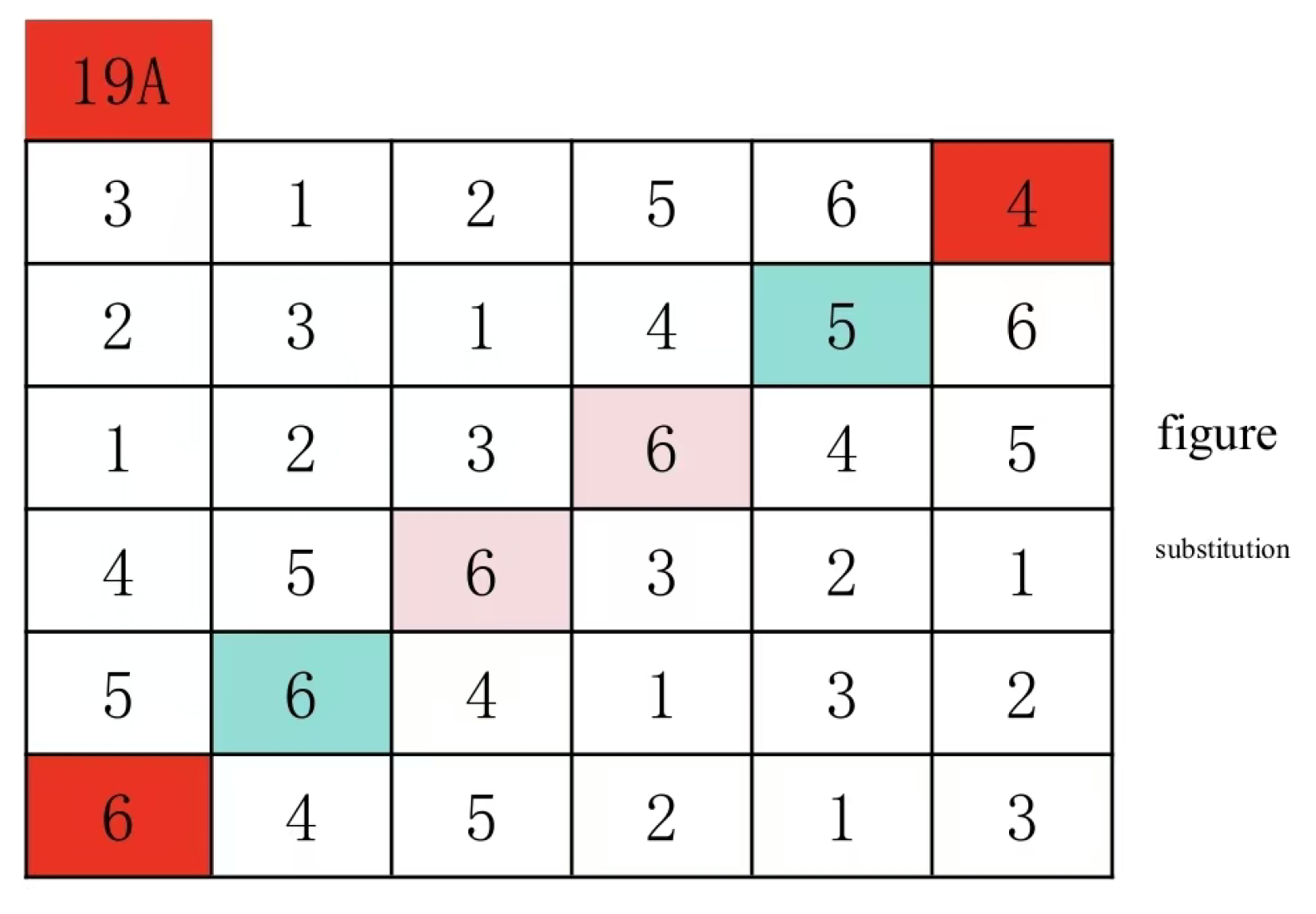
Figure 21 shows the correspondence between paired groups (6:4) and (6:5) in Latin squares, while Figure 19 illustrates the same relationship for paired groups (4:6) and (4:5). This correspondence establishes that numbers 4 correspond to number 6, 1 to number 1, 2 to number 2, and 5 to number 5. By continuing this process with subsequent paired groups along the secondary mainline until all pairs are completed, we can align the modulo forms of the secondary mainlines in both Latin squares. This entire process can be completed within polynomial time, with a time complexity of $5/16(n^5-2n^4-n^3+2n^2)+2n^3$

While this step is standard practice (as most would recognize), I’ll still outline the original algorithm since it boasts lower time complexity. The core mechanism remains unchanged: when processing symbols in two Latin squares, the primary alignment group structure stays consistent, while the numerical permutation groups remain stable. However, the relationship between outer and inner groups within the same group structure becomes problematic. Although previously noted as inherently unstable, this scenario appears manageable. Through practical implementation, I discovered that aligning secondary alignment patterns across Latin squares proves effective. When secondary alignment patterns differ in modulo form, simply switch to another matching pattern. This approach directly identifies congruent secondary alignment patterns between Latin squares, likely due to their inherent properties. This discovery has fueled my ongoing exploration of deeper structural characteristics within Latin square systems. The proof process remains incomplete and will not be elaborated here.

6. A Fast and Accurate Algorithm for Filling the Square Grid

Given a Latin grid to be filled, it can be transformed into a line specification type. This approach enables the creation of N distinct group structures corresponding to N different group configurations. The system can efficiently generate group configurations satisfied by a symbol as the main line.However, the number of such group configurations depends on the quantity of given symbols. Given that N symbols form the main line configuration, these group structures should exhibit interconnections within the Latin grid. What are the relationships between external and internal connections among these group structures? I am currently conducting research by unfolding the Latin grid for analysis.These two challenges constitute the primary obstacles in solving the algorithm: 1. Uncertainty about which specific group configuration exists in the Latin grid to be filled; 2. Understanding the intergroup relationships (both external and internal) between groups. Solving this problem requires polynomial-time computation, as detailed in the first category of Latin grid generation algorithms within the precise counting framework. This demonstrates the connection between #P-complete and NP-complete problems, as both represent fundamental barriers in the counting domain. Therefore, I believe the key to resolving NP-complete issues lies precisely here.

While the two connections mentioned above remain unknown, I have developed alternative approaches. Since these constitute the primary barriers, we should focus on addressing them. To efficiently identify permutation sets, we generate all N×N Latin squares with non-repetitive row-column exchanges. The optimized generation algorithm strategy involves initially placing known permutation sets into the initial phase, then proceeding through similar algorithmic steps. As previously noted, there’s no need to fully construct all permutation set structures in the construction area. Identifying the minimal set of permutation structures would significantly accelerate the algorithm. Regarding inter-group and intra-group relationships, we employ the construction area filling techniques from earlier algorithms to speed up computations. Since the solution algorithm and generation algorithm are mutually reinforcing, their mechanisms won’t be elaborated here. The time complexity will remain undisclosed as potential optimizations may emerge if these connections are identified.

7. Summary and Description

While some conjectures in this paper remain unresolved, they do not affect the conclusions. Their resolution would be ideal, which will constitute one of my future research priorities. My main focus will continue to be deriving precise counting formulas for Latin squares and optimizing algorithms for rapid solving of pending Latin square problems - essentially seeking connections between these areas. These challenges persist due to their immense computational demands and limited applicable conclusions, often requiring me to tackle them alone. The text incorporates numerous novel terms and concepts, avoiding standard academic jargon to maintain clarity. To mitigate potential information loss during machine translation, I have included diagrams and detailed algorithmic steps, ensuring both human comprehension and accuracy in machine-translated outputs.

The algorithm proposed in this paper may be submitted for patent protection in the future. To avoid potential adverse impacts, academic use, dissemination, and exchange of this algorithm, as well as its fair use in compliance with relevant norms, are fully permitted. If there are any deficiencies in this paper, they will be further revised and improved in subsequent research. Furthermore, academic breakthroughs require overcoming unimaginable pressures and difficulties, and are also inseparable from the protection and support of all parties. It is earnestly requested that all sectors respect my research work.

References

- Euler, L. Recherches sur un nouvelle espéce de quarrés magiques. Verhandelingen uitgegeven door het zeeuwsch Genootschap der Wetenschappen te Vlissingen 1782, 85–239. [Google Scholar]
- Valiant, L.G. The complexity of computing the permanent. Theoretical computer science 1979, 8, 189–201. [Google Scholar] [CrossRef]
- Keedwell, A.D.; Dénes, J. Latin Squares and Their Applications: Latin Squares and Their Applications; Elsevier, 2015. [Google Scholar]
- Jerrum, M.; Sinclair, A. Fast uniform generation of regular graphs. Theoretical Computer Science 1990, 73, 91–100. [Google Scholar] [CrossRef]
- Hulpke, A.; Kaski, P.; Östergård, P. The number of Latin squares of order 11. Mathematics of computation 2011, 80, 1197–1219. [Google Scholar] [CrossRef]
- McKay, B.D.; Meynert, A.; Myrvold, W. Small Latin squares, quasigroups, and loops. Journal of Combinatorial Designs 2007, 15, 98–119. [Google Scholar] [CrossRef]
- Collins, N.A.; Grochow, J.A.; Levet, M.; Weiß, A. Constant depth circuit complexity for generating quasigroups. In Proceedings of the Proceedings of the 2024 International Symposium on Symbolic and Algebraic Computation; 2024; pp. 198–207. [Google Scholar]
- Wolf, M.J. Nondeterministic circuits, space complexity and quasigroups. Theoretical Computer Science 1994, 125, 295–313. [Google Scholar] [CrossRef]
- Chattopadhyay, A.; Torán, J.; Wagner, F. Graph isomorphism is not AC0-reducible to group isomorphism. ACM Transactions on Computation Theory (TOCT) 2013, 5, 1–13. [Google Scholar] [CrossRef]
- Levet, M. On the complexity of identifying strongly regular graphs. arXiv 2022, arXiv:2207.05930. [Google Scholar]
- Miller, G.L. On the nlog n isomorphism technique (a preliminary report). In Proceedings of the Proceedings of the tenth annual ACM symposium on theory of computing; 1978; pp. 51–58. [Google Scholar]
- Ivanyos, G.; Qiao, Y. Algorithms based on*-algebras, and their applications to isomorphism of polynomials with one secret, group isomorphism, and polynomial identity testing. SIAM Journal on Computing 2019, 48, 926–963. [Google Scholar] [CrossRef]
- Grochow, J.; Qiao, Y. On the complexity of isomorphism problems for tensors, groups, and polynomials I: tensor isomorphism-completeness. SIAM Journal on Computing 2023, 52, 568–617. [Google Scholar] [CrossRef]
- Colbourn, C.J. The complexity of completing partial latin squares. Discrete Applied Mathematics 1984, 8, 25–30. [Google Scholar] [CrossRef]
Disclaimer/Publisher’s Note: The statements, opinions and data contained in all publications are solely those of the individual author(s) and contributor(s) and not of MDPI and/or the editor(s). MDPI and/or the editor(s) disclaim responsibility for any injury to people or property resulting from any ideas, methods, instructions or products referred to in the content. |
© 2025 by the authors. Licensee MDPI, Basel, Switzerland. This article is an open access article distributed under the terms and conditions of the Creative Commons Attribution (CC BY) license (http://creativecommons.org/licenses/by/4.0/).
Copyright: This open access article is published under a Creative Commons CC BY 4.0 license, which permit the free download, distribution, and reuse, provided that the author and preprint are cited in any reuse.