Submitted:
01 October 2025
Posted:
01 October 2025
You are already at the latest version
Abstract
In a cellular maritime communication system, ocean buoys are essential to enable environmental monitoring, offshore platform management, and disaster response. Therefore, energy efficient transmission from the buoys is a key requirement to prolong their operational time. A fixed uplink beamforming can be considered to save energy by leveraging its beam gain while managing the target link reliability. However, the dynamic condition of ocean waves causes buoy’s random orientation, leading to frequent misalignment of its predefined beam direction aimed at the base station which degrades both the link reliability and energy efficiency. To address this challenge, we propose a wave-adaptive beamforming framework to satisfy data-rate demands within limited power budgets. This strategy targets scenarios where sea state information is unavailable, such as in network-assisted systems.We propose a Two-Dimensional Thompson Sampling (2DTS) scheme that jointly selects beamwidth and transmit power to satisfy the target-rate constraint with minimal power consumption and thus achieve maximal energy efficiency. This adaptive learning approach effectively balances exploration and exploitation, enabling efficient operation in uncertain and changing sea conditions. The simulation results demonstrate that the strategy enhances energy efficiency, confirming its practicality for maritime communication systems constrained by limited power budgets.
Keywords:
maritime communication
; 2DTS
; beam management
; energy efficiency
1. Introduction
The growing demand for advanced maritime applications, such as surveillance, environmental monitoring, offshore platform management, and disaster response services, requires buoy-based ocean communication networks [1,2]. In particular, lighthouses and maritime buoy now play a critical role, going beyond simple signaling to transmitting real-time environmental and situational data including wave height, surrounding visibility, and environmental video feeds. These high data rate requirements necessitate more efficient wireless transmission strategies than the low-rate, omnidirectional links traditionally used for basic telemetry (e.g., wave height, air temperature).
Unlike terrestrial networks, maritime communication systems must deal with a highly dynamic ocean environment. Waves, wind and currents induce buoy motions that tilt, heave and rotate, increasing the probability of outage and the increase of energy consumption [3]. Although these effects are governed by the sea state, real time sea state information is often unavailable. As a result, static power allocation schemes often result in inefficiencies in spectral and energy resources [4]. To address this, recent studies have explored adaptive techniques such as beamforming and multi-hop relaying to strengthen maritime links [5,6]. While directional beamforming can focus energy toward the intended receiver [7], most existing methods presume prior knowledge of sea conditions at the buoys, limiting their utility in the use cases when the sea conditions or channel state information are not available [8,9]. A key limitation of these schemes is that buoys typically have only limited knowledge of the prevailing sea state for uplink beamforming, whereas the BS can infer sea-state dynamics more reliably from satellite-based, wide-area forecasts. Moreover, it is noted that the instantaneous beamforming that adopts to changing orientation of the buoy requires the channel state information feedback from the base station, where cellular maritime communication such as LTE-M lacks of MIMO framework.
To address this challenge with respect to the uncertainty of the sea state and its related feedback channel unavailability in the current marine cellular system, we propose an adaptive beam and power control method based on Thompson sampling (TS) based reinforcement learning [10] without knowledge on the sea state directly from the base station. Because the base station cannot have knowledge on the sea state directly, we exploit the feedback information to implicitly infer the current sea state. To optimize beamwidth and power allocation under uncertain conditions, we employ Thompson Sampling (TS) framework, a Bayesian algorithm widely used in multi-armed bandit (MAB) problems [11,12,13]. TS is known that efficiently balances exploration and exploitation by sampling from the posterior belief distributions of each action. Especially, the posterior is updated based on binary feedback success or failure, while allowing the algorithm to gradually converge to the most promising actions. TS has been successfully applied in areas such as online advertising, recommendation systems, and clinical trials. In communication systems, it has been used for channel selection, interference management, and power control, including underwater acoustic communications and dynamic spectrum access [13,14].
Unfortunately, most of the above mentioned applications focus on maximizing performance metrics like throughput or reliability, with limited attention to energy efficiency [15]. Unlike these existing applications, in our scenario, beamforming performance is highly sensitive to sea state conditions, where dynamic wave motion causes variations in signal alignment and channel quality. Alongside strict power constraints at buoys, this creates a multi-dimensional optimization problem involving both beamwidth and transmit power, which makes standard TS not suitable for our problem. To overcome these limitations, we develop novel Two-Dimensional Thompson Sampling (2DTS). The goal of 2DTS is to jointly select the optimal beamwidth and the minimum transmission power required to meet a predefined target data rate. This is achieved by updating the shape parameters and of the posterior beta distribution for each beamwidth and power pair selection actions, using binary feedback from the base station indicating whether the target rate was successfully achieved. This approach enables adaptive learning that accounts for underlying sea state variations while minimizing power consumption. By integrating 2DTS into our framework, we provide an efficient solution that balances exploration and exploitation, ensuring reliable and energy-efficient communication in dynamic and uncertain maritime environments.
The paper is organized as follows. Section II models wave-induced fluctuations in the uplink transmit beam gain by incorporating buoy motion and sea-surface dynamics. Section III presents the Two-Dimensional Thompson Sampling (2DTS) algorithm, which jointly selects beamwidth and transmit power to meet the target-rate constraint with minimal power, thereby maximizing energy efficiency. Section IV reports simulation results that validate the modeling and quantify the gains of the proposed approach. Finally, Section V concludes the paper.
2. System Model
As illustrated in Figure 1, we consider an uplink maritime communication scenario where a buoy equipped with N transmit antennas communicates with a single-antenna base station (BS). The buoy’s location and orientation are assumed known, so the buoy employs predefined fixed transmit beamforming aiming at the base station without dynamic adjustments. The buoy transmits the scalar information symbol to the BS through a linear beamforming vector . Accordingly, the received signal vector, denoted as at the BS is represented as
where is the channel between the buoy and BS, and follows an additive white Gaussian noise (AWGN) distribution. For simplicity, is chosen from a predefined vertical beam vector set , where they are the arrays steering to BS with different vertical beamwidths. It is assumed that the uplink beam vectors are designed to be horizontally isotropic and vertically directional because it can frequently be rotating due to the ocean current. indicates the beamforming vector with beamwidth , and subsequent beamwidths are progressively halved, given by
corresponding to and . For modeling the channel , following [16], we assume
where and represent the Line-of-Sight (LoS) and the Non Line-of-Sight (NLoS) components of the channel, respectively. For the NLoS component, we assume that each element in is drawn from . This part captures the scattered multipath components. The Rician factor K represents the ratio of the power in the LoS component to the power in the NLoS component. The LoS component, , reflects the deterministic nature of the direct transmission path, which is particularly dominant in the maritime environment due to the lack of obstacles between the BS and the buoy [17]. Although the buoy is placed at known locations, the sea surface moves dynamically and causes the buoy orientation changes, resulting in misalignment of the direction of the transmit array of the buoy and degradation of the gain at BS [18].
2.1. Statistical Modeling of Ocean Beam Channel
Incorporating the dynamic ocean environment into the channel model, the modified channel is expressed as
where
where is the angle of departure at buoy and is derived from the buoy’s angular displacement caused by ocean wave dynamics modeled via the ISSC spectrum [3]. To account for the impact of the beamwidth on the overall channel performance, the effective channel gain is defined as the projection of the channel vector onto the beamforming vector. Specifically, the effective channel gain is expressed as:
where denotes the effective channel gain after considering the effects of the dynamic ocean environment, and represents the beamforming vector corresponding to a specific beamwidth. In high sea states, large wave heights induce substantial angular variations of the buoy, thereby increasing the probability of steering misalignment, particularly when employing narrower transmit beams. While a narrower beam can provide larger array gain, its susceptibility to misalignment may severely degrade system performance under adverse conditions. Consequently, the buoy must adapt its beam vector to preserve robustness against wave-induced motion in the current sea state. The optimal beamwidths and the corresponding minimum transmit powers required to meet the target across different sea states are summarized in Table 1.
3. Joint Beamwidth and Power Selection Using 2DTS
This section introduces a joint beamwidth and power selection strategy for maritime communication using 2DTS. In scenarios where the sea state information is known at the buoy, effective adaptation is crucial. Unlike the Upper Confidence Bound(UCB) algorithm,which struggles under dynamic conditions due to its reliance on confidence intervals,TS achieves a better balance between exploration and exploitation through probabilistic sampling. The proposed approach extends standard TS by jointly selecting the best beamwidth and minimum transmit power. enabling network-assisted real-time adaptation to varying maritime environments. Simulation shows that 2DTS outperforms standard TS, leading to lower power consumption, higher reliability, and robust operation under dynamic and uncertain sea states.
3.1. Standard Thompson Sampling
Thompson Sampling (TS) is a popular Bayesian decision-making algorithm tailored for uncertain environments, particularly effective in MAB problems. The fundamental objective in a MAB setting is to maximize cumulative rewards by choosing among K possible actions (or arms), each with an unknown reward distribution. TS accomplishes this by sampling from posterior distributions of the reward means and updating these distributions as new data (rewards) are observed. Over time, it allocates resources to actions believed to yield higher returns while still periodically exploring other actions to gather new information. Below, we provide an expanded description of TS, emphasizing the Bayesian structure and adaptive update rules.
3.1.1. Bayesian Multi-Armed Bandit Formulation
Consider a MAB with K arms, where each arm is associated with an unknown reward distribution. Let denote the (unknown) mean reward of arm k. The agent, or decision-maker, seeks to maximize the cumulative reward obtained by sequentially selecting arms over T rounds. At each round t, the agent selects an arm , observes a reward drawn from the distribution with mean , and subsequently updates its posterior belief about based on the observed reward. The central challenge lies in balancing exploration of insufficiently understood arms with exploitation of arms already identified as yielding high rewards.
3.1.2. Bayesian Perspective and Thompson Sampling Logic
From a Bayesian standpoint, each mean reward is modeled with a prior distribution that reflects initial uncertainty. As rewards are observed, Bayes’ rule is applied to update this belief, yielding a posterior distribution . Thompson Sampling exploits this posterior by sampling a candidate value of for each arm and selecting the arm with the highest sampled value. This naturally balances exploration and exploitation, as arms with uncertain but potentially high means can still be chosen. The procedure can be described step by step as follows.
- 1)
- Initialization.
Define a prior distribution for each arm . The choice of prior depends on the reward type:
- For Bernoulli rewards (i.e., rewards are either 0 or 1), a beta distribution is typically selected:where and are positive hyperparameters. This is because the beta distribution is the conjugate prior for the Bernoulli likelihood, ensuring a simple form of posterior updates.
- For Gaussian rewards, a normal prior is often chosen:where is the initial mean, and is the initial variance. The normal distribution is a conjugate prior for the Gaussian likelihood, which keeps posterior updates tractable.
These priors capture the agent’s initial beliefs about the reward means before any data is observed.
- 2)
- Sampling.
In each round t, for each arm , sample a reward estimate from the posterior distribution . This posterior reflects the agent’s updated knowledge after previous selections. Concretely:
-
Bernoulli rewards (Beta prior):where is the total number of observed “successes” (reward = 1) and the total number of observed “failures” (reward = 0) for arm k. Each time arm k is played, the parameters are updated accordingly.
-
Gaussian rewards (Normal prior):Here, is the sum of all rewards observed from arm k, is the number of times arm k has been selected, and is the known variance of the underlying reward distribution.
By drawing a sample from each posterior, TS naturally incorporates both the estimated mean and associated uncertainty.
- 3)
- Action Selection.
After sampling one candidate for each arm k, the algorithm chooses the arm
Thus, the selected arm is the one that this particular sample indicates has the largest mean reward. Over many rounds, arms with higher posterior means or lower uncertainty will be chosen more often, but less-known arms still have a chance to be sampled if their posterior draws occasionally exceed those of well-explored arms.
- 4)
- Update.
The chosen arm is played, and the resulting reward is observed. The posterior for is then updated according to Bayesian rules:
- Bernoulli rewards: If , update
- Gaussian rewards: Update the mean and variance parameters of the normal posterior using standard Gaussian conjugate updating formulas, incorporating the new data point .
This feedback loop is repeated in each subsequent round, enabling the algorithm to progressively refine its understanding of each arm’s reward potential.
3.2. Problem Formulation
In this paper, the objective is to select the beamwidth and the transmit power level so that the achieved rate meets or exceeds a predefined threshold while minimizing the power used. To achieve this, we utilized 2DTS to select the best beamwidth and minimum power level.
Let denote the available beamwidth options, where , and denote the available power levels, where . The objective is to maximize the cumulative number of successful transmissions over multiple trials while minimizing energy consumption.
3.3. Thompson Sampling with Joint Beamwidth and Power Selection
We apply 2DTS to jointly select the beamwidth and the power level in each trial to find the beamwidth and the minimum power that meet a given rate threshold r. The algorithm operates as follows:
- Initialize the parameters and for the beta distribution for each beamwidth i and each power level j, with , , , and for all i and j.
-
For each trial t:
- -
- Sample from for each beamwidth i.
- -
- Select the beamwidth with the highest sampled value:
- -
-
For the selected beamwidth , the power value corresponding to the maximum sampled probability from the beta distribution from for each power level j, then select the power level with the highest sampled value:The algorithm selects the power level aiming to minimize power usage by choosing the lowest possible power level that still satisfies the target threshold r. Here, denotes the instantaneous channel capacity, while the threshold r is set strictly below this maximum capacity to represent the actual transmission rate. Thus, the algorithm checks whether the achievable rate exceeds r, treating r as the success criterion for transmission.
- -
- Calculate the SNR for the selected beamwidth and power level:where is the effective channel gain associated with beamwidth and N is the noise power. Using this SNR, compute the rate as:
- -
- Determine the reward based on whether the achievable rate meets or exceeds the target threshold r:
- -
-
Update the beta distribution parameters for the selected beamwidth and power level based on the observed reward:
- *
- For the selected beamwidth :
- *
-
For the selected power level of the selected beamwidth :
- .
- If , it means success (the rate threshold is met or exceeded), increase for the selected power level and the level immediately below it (if it exists). This update encourages the selection of lower power levels that can meet the threshold, improving power efficiency:
- .
- If , it means fail (the rate threshold is not met), increase for the selected power level and all power levels below it. This penalizes lower power levels that fail to meet the threshold, encouraging the selection of higher power levels when necessary:
In this approach, 2DTS iteratively updates its estimates of the success probabilities for each power level, allowing it to identify the minimum power level that achieves the required rate with high confidence. Adjusting and for each beamwidth and power level based on observed rate, the algorithm efficiently balances exploration and exploitation, focusing on power levels that maximize energy efficiency while meeting the communication threshold.
| Algorithm 1: 2DTS for Beamwidth and Power selection |
|
3.4. Energy Efficiency
We confirmed the proposed 2DTS joint beamwidth–power selection over T trials. At each trial t, 2DTS samples a beam and a power. The cumulative number of successful transmissions at trial t is
where denotes the binary reward at round t.. The cumulative power used over T trials is
Accordingly, the overall energy efficiency after T trials is
Equivalently, 2DTS seeks to maximize over the sequence :
The results indicate that the algorithm successfully converges to the optimal beamwidth and power level, achieving reliable communication with minimum energy consumption.
4. Simulation Results
In this section, we present simulation results that quantitatively demonstrate the effectiveness of the proposed 2DTS algorithm in selecting the optimal beamwidth and transmit power under varying sea states. Performance is measured in terms of cumulative energy efficiency () in iterative rounds. Figure 2 and Figure 3 show the energy efficiency achieved by four schemes: (i) an ideal case that assumes perfect prior knowledge of the optimal beamwidth and power at each round, (ii) the proposed 2DTS algorithm, (iii) a modified TS with a dedicated exploration phase, and (iv) a conventional TS that independently selects beamwidth and power using standard TS. Figure 2, under moderate sea state (sea state 4), the proposed 2DTS achieves an energy efficiency of approximately (r/p) at round 600, which is 73.5% of the ideal case performance ( (r/p)). This result clearly outperforms both the exploration-based variant () and the conventional TS (), indicating relative gains of 96.9% and 447.8% over the exploration-based and conventional TS baselines, respectively. Figure 3, for a harsh sea state (sea state 9), the performance gap narrows further. In round 600, 2DTS achieves , corresponding to 85.6% of the ideal case (), while exploration TS and conventional TS reach and , respectively. This translates to a performance gain of 84.0% over conventional TS, again highlighting the robustness of the 2DTS framework in dynamically fluctuating maritime environments. The superior performance of 2DTS arises from its joint optimization structure. Unlike standard TS, which treats each parameter selection problem independently, our 2DTS algorithm simultaneously selects the optimal beamwidth and power pair through a joint posterior update that incorporates both the directional gain dynamics (affected by beamwidth) and power efficiency trade-offs. This structure is specifically tailored for maritime systems where beam misalignment and power constraints are tightly coupled due to wave-induced platform motion.
Especially, to the best of our knowledge, no existing TS-based algorithm directly addresses the joint selection of beamwidth and power levels under unknown and dynamic sea-state conditions. Although advanced variants of TS (e.g., contextual or neural TS) have been proposed in other domains, they are generally not suitable for the maritime scenario considered in this work. In our setting, the decision space is discrete and multidimensional, and it is tightly coupled with physical constraints like beam misalignment and energy efficiency. Therefore, our approach constitutes a novel formulation of TS tailored to this setting, offering a practical solution in the absence of sea-state information. In summary, 2DTS achieves up to 85.6% of ideal energy efficiency in varying sea states, while significantly outperforming baseline methods, demonstrating its suitability for energy-constrained maritime communication environments.
5. Conclusion
In this work, we proposed an adaptive approach for buoy-embedded maritime communication systems, focusing on the selection of beamforming and power control under dynamic sea conditions. For unknown sea states, we developed a novel 2DTS algorithm that simultaneously adjusts beamwidth and transmission power, achieving robust communication even without direct sea state information. This adaptive framework balances exploration and exploitation to optimize communication parameters over time, closely approximating ideal performance, and ensuring energy-efficient operation. Our simulation results validate the effectiveness of this method, demonstrating significant improvements in energy efficiency and reliability in dynamic maritime environments. Our approach advances the field of maritime communications by providing a robust, energy-efficient strategy for dynamic and unpredictable sea conditions.
Author Contributions
Conceptualization, K.J.L. (KyeongJea Lee) and D.K.K.; methodology, K.J.L. (KyeongJea Lee); software, K.J.L. (KyeongJea Lee); validation, J.-H.J. and D.K.K.; writing—original draft, K.J.L. (KyeongJea Lee); writing—review and editing, J.-H.J., S.C., K.-W.K., and D.K.K.; supervision, D.K.K.
Funding
This research was supported by Korea Institute of Marine Science and Technology Promotion(KIMST), funded by the Ministry of Oceans and Fisheries, grant number RS-2021-KS211516.
Institutional Review Board Statement
Not applicable.
Informed Consent Statement
Not applicable.
Data Availability Statement
Data supporting the findings of this study are available from the corresponding author upon reasonable request.
Acknowledgments
This research was supported in part by Korea Institute of Marine Science and Technology Promotion (KIMST) grant funded by the Ministry of Oceans and Fisheries under Grant RS-2021-KS211516 and RS-2023-00238653.
Conflicts of Interest
The authors declare no conflict of interest.
References
- Palma, D. Enabling the Maritime Internet of Things: CoAP and 6LoWPAN Performance Over VHF Links. IEEE Internet of Things J. 2018, 5, 5205–5212. [Google Scholar] [CrossRef]
- Yang, T.; Zheng, Z.; Liang, H.; Deng, R.; Cheng, N.; Shen, X. Green Energy and Content-Aware Data Transmissions in Maritime Wireless Communication Networks. IEEE Trans. Intell. Transp. Syst. 2015, 16, 751–762. [Google Scholar] [CrossRef]
- Huo, Y.; Dong, X.; Beatty, S. Cellular Communications in Ocean Waves for Maritime Internet of Things. IEEE Internet of Things J. 2020, 7, 9965–9979. [Google Scholar] [CrossRef]
- Zhou, Z.; Ge, N.; Wang, Z. Two-Timescale Beam Selection and Power Allocation for Maritime Offshore Communications. IEEE Commun. Lett. 2021, 25, 3060–3064. [Google Scholar] [CrossRef]
- Guan, S.; Wang, J.; Jiang, C.; Duan, R.; Ren, Y.; Quek, T.Q.S. MagicNet: The Maritime Giant Cellular Network. IEEE Commun. Mag. 2021, 59, 117–123. [Google Scholar] [CrossRef]
- Kim, H.J.; Tiwari, S.V.; Chung, Y.H. Multi-hop relay-based maritime visible light communication. Chin. Opt. Lett. 2016, 14, 050607. [Google Scholar] [CrossRef]
- Wang, W.; Gill, E.W. Evaluation of Beamforming and Direction Finding for a Phased Array HF Ocean Current Radar. J. Atmos. Ocean. Technol. 2016, 33, 2599–2613. [Google Scholar] [CrossRef]
- Romdhane, I.; Kaddoum, G. A Reinforcement-Learning-Based Beam Adaptation for Underwater Optical Wireless Communications. IEEE Internet of Things J. 2022, 9, 20270–20281. [Google Scholar] [CrossRef]
- Jo, S.W.; Shim, W.S. LTE-Maritime: High-Speed Maritime Wireless Communication Based on LTE Technology. IEEE Access. 2019, 7, 53172–53181. [Google Scholar] [CrossRef]
- Ibrahim, S.; Mostafa, M.; Jnadi, A.; Salloum, H.; Osinenko, P. Comprehensive Overview of Reward Engineering and Shaping in Advancing Reinforcement Learning Applications. IEEE Access. 2024, 12, 175473–175500. [Google Scholar] [CrossRef]
- Russo, D.J.; Roy, B.V.; Kazerouni, A.; Osband, I.; Wen, Z. A Tutorial on Thompson Sampling. Foundations and Trends in Machine Learning. 2018, 11, 1–96. [Google Scholar] [CrossRef]
- Chapelle, O.; Li, L. An Empirical Evaluation of Thompson Sampling. In Proceedings of the Advances in Neural Information Processing Systems; Shawe-Taylor, J.; Zemel, R.; Bartlett, P.; Pereira, F.; Weinberger, K., Eds. Curran Associates, Inc., 2011, Vol. 24. [CrossRef].
- Deng, W.; Kamiya, S.; Yamamoto, K.; Nishio, T.; Morikura, M. Thompson Sampling-Based Channel Selection Through Density Estimation Aided by Stochastic Geometry. IEEE Access. 2020, 8, 14841–14850. [Google Scholar] [CrossRef]
- Tong, J.; Fu, L.; Wang, Y.; Han, Z. Model-Based Thompson Sampling for Frequency and Rate Selection in Underwater Acoustic Communications. IEEE Trans. Wireless Commun. 2023, 22, 6946–6961. [Google Scholar] [CrossRef]
- Komiyama, J.; Honda, J.; Nakagawa, H. Optimal Regret Analysis of Thompson Sampling in Stochastic Multi-armed Bandit Problem with Multiple Plays 2015. 37, 1152–1161. [CrossRef].
- Duan, R.; Wang, J.; Zhang, H.; Ren, Y.; Hanzo, L. Joint Multicast Beamforming and Relay Design for Maritime Communication Systems. IEEE Trans. Green Commun. Netw. 2020, 4, 139–151. [Google Scholar] [CrossRef]
- Wang, J.; Zhou, H.; Li, Y.; Sun, Q.; Wu, Y.; Jin, S.; Quek, T.Q.S.; Xu, C. Wireless Channel Models for Maritime Communications. IEEE Access. 2018, 6, 68070–68088. [Google Scholar] [CrossRef]
- Yau, K.L.A.; Syed, A.R.; Hashim, W.; Qadir, J.; Wu, C.; Hassan, N. Maritime Networking: Bringing Internet to the Sea. IEEE Access. 2019, 7, 48236–48255. [Google Scholar] [CrossRef]
Figure 1.
The system model.
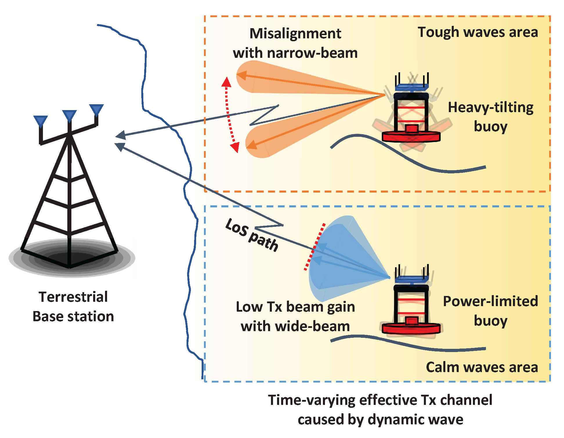
Figure 2.
Energy efficiency over rounds (sea state 4).
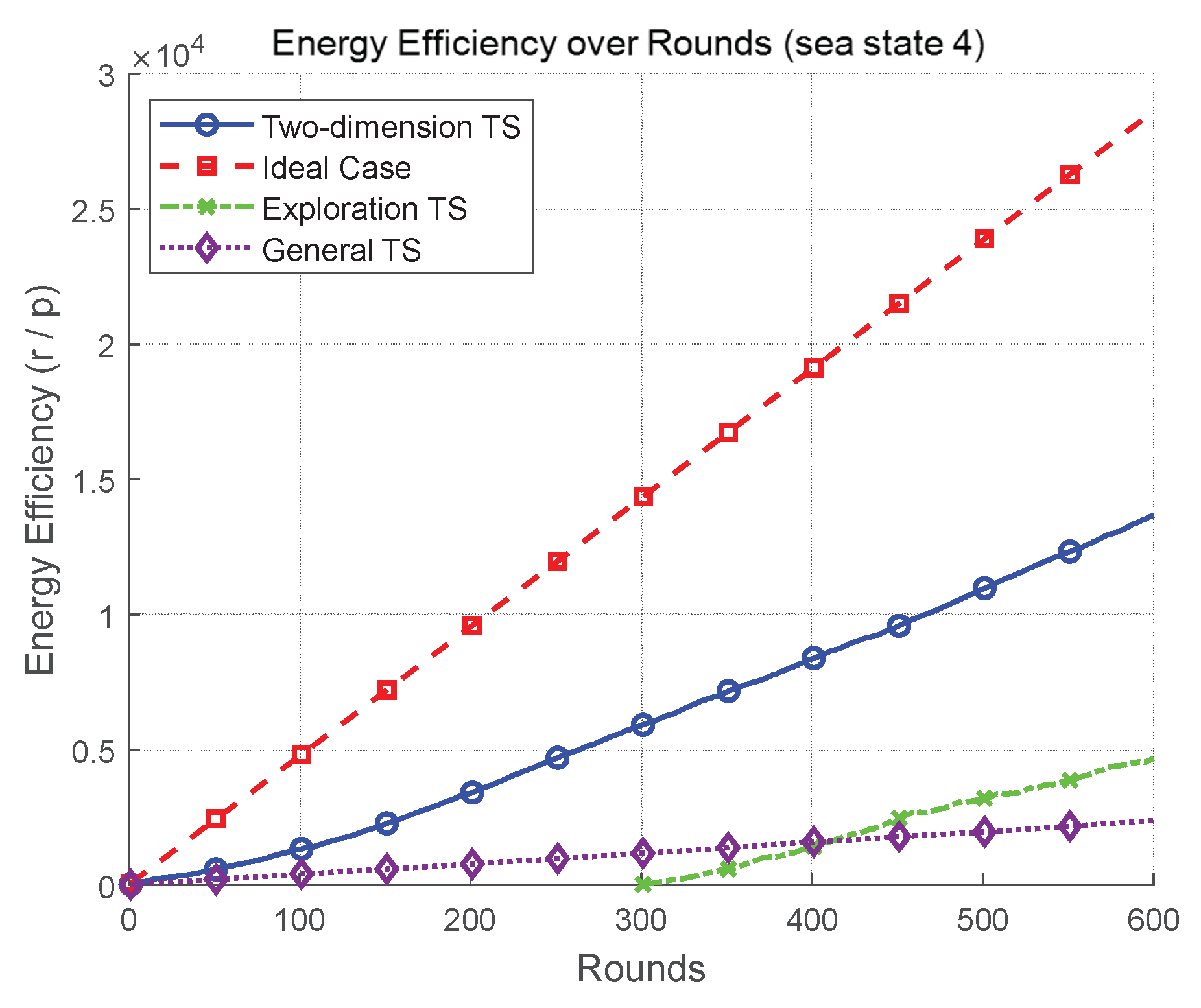
Figure 3.
Energy efficiency over rounds (sea state 9).
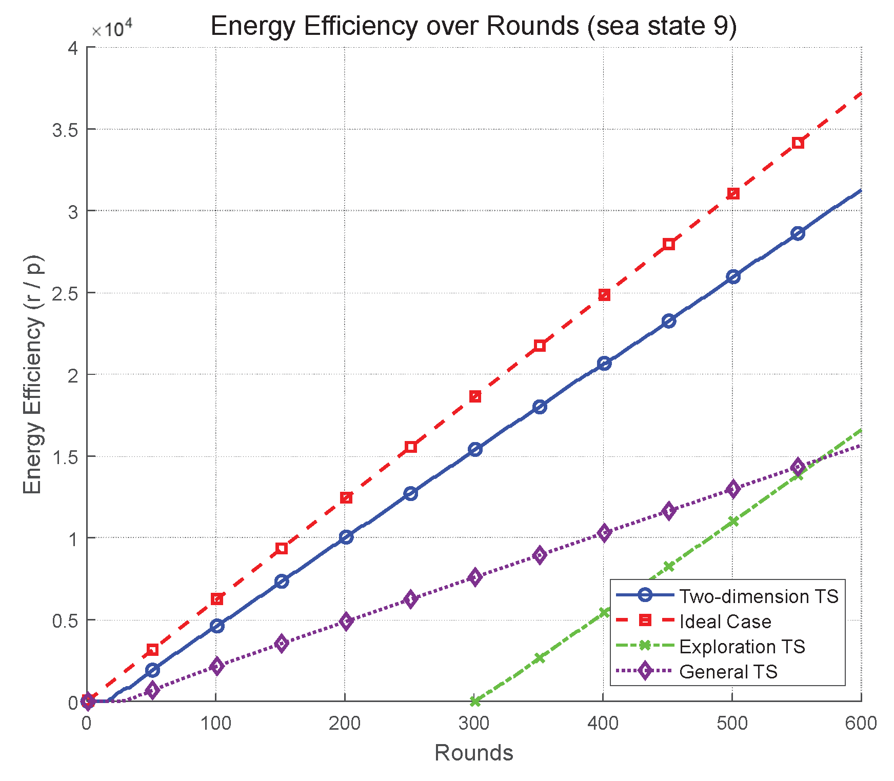

Table 1.
Optimal Beamwidth and Minimum Power Required per Sea State.
| Sea State | Optimal Beamwidth (°) | Minimum Power (W) |
|---|---|---|
| 1 | 2.81 | 0.0013 |
| 2 | 5.62 | 0.0031 |
| 3 | 11.25 | 0.0106 |
| 4 | 11.25 | 0.0304 |
| 5 | 22.50 | 0.0416 |
| 6 | 22.50 | 0.0563 |
| 7 | 22.50 | 0.0779 |
| 8 | 45.00 | 0.1373 |
| 9 | 45.00 | 0.1625 |
Note: Values are computed for a target rate of 6 bps/Hz.
Disclaimer/Publisher’s Note: The statements, opinions and data contained in all publications are solely those of the individual author(s) and contributor(s) and not of MDPI and/or the editor(s). MDPI and/or the editor(s) disclaim responsibility for any injury to people or property resulting from any ideas, methods, instructions or products referred to in the content. |
© 2025 by the authors. Licensee MDPI, Basel, Switzerland. This article is an open access article distributed under the terms and conditions of the Creative Commons Attribution (CC BY) license (http://creativecommons.org/licenses/by/4.0/).
Copyright: This open access article is published under a Creative Commons CC BY 4.0 license, which permit the free download, distribution, and reuse, provided that the author and preprint are cited in any reuse.


