
Submitted:
29 September 2025
Posted:
30 September 2025
You are already at the latest version
Abstract
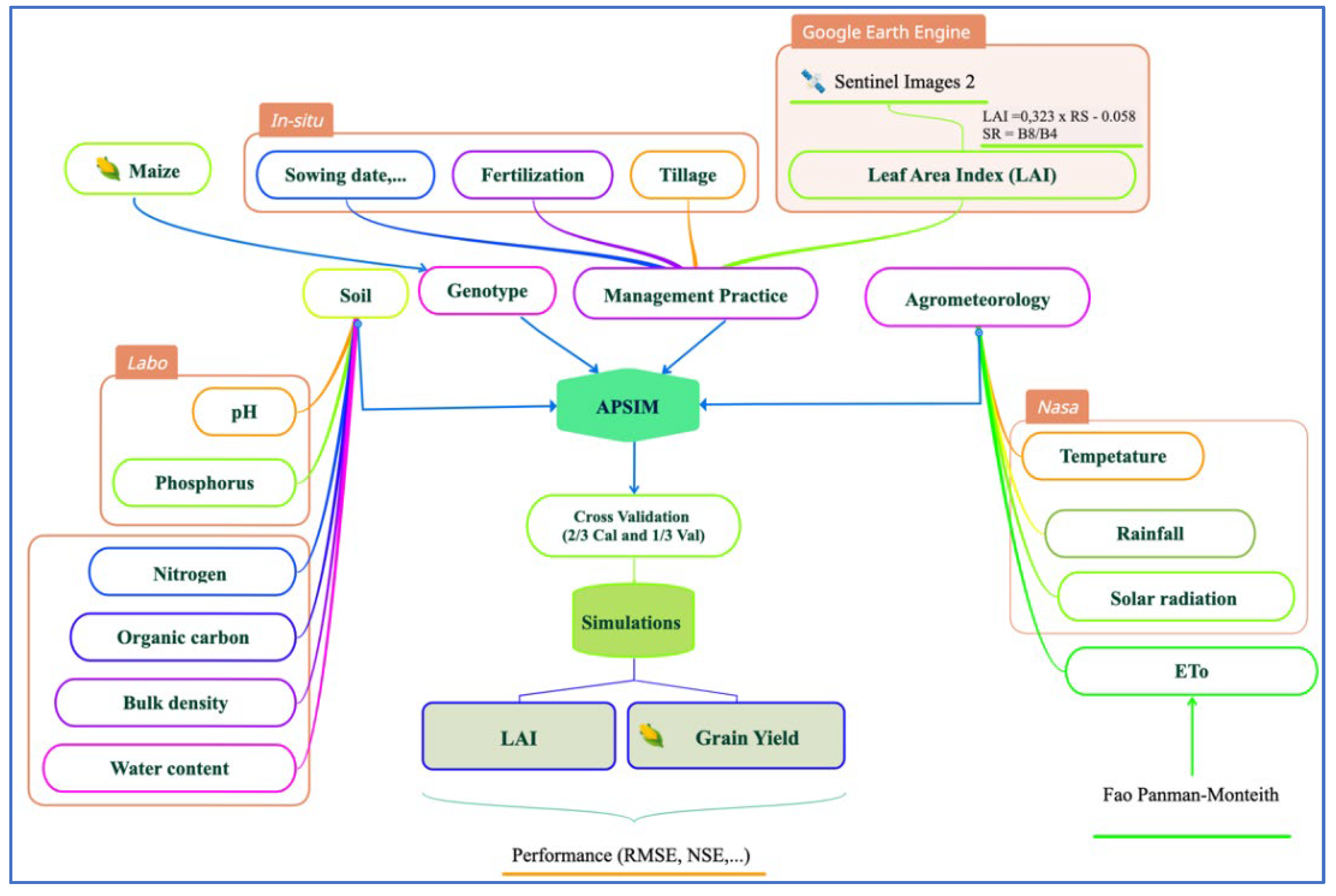
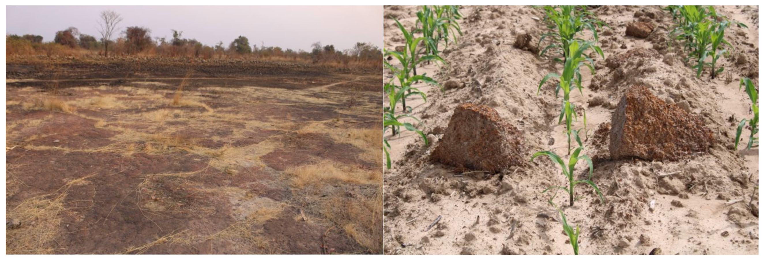
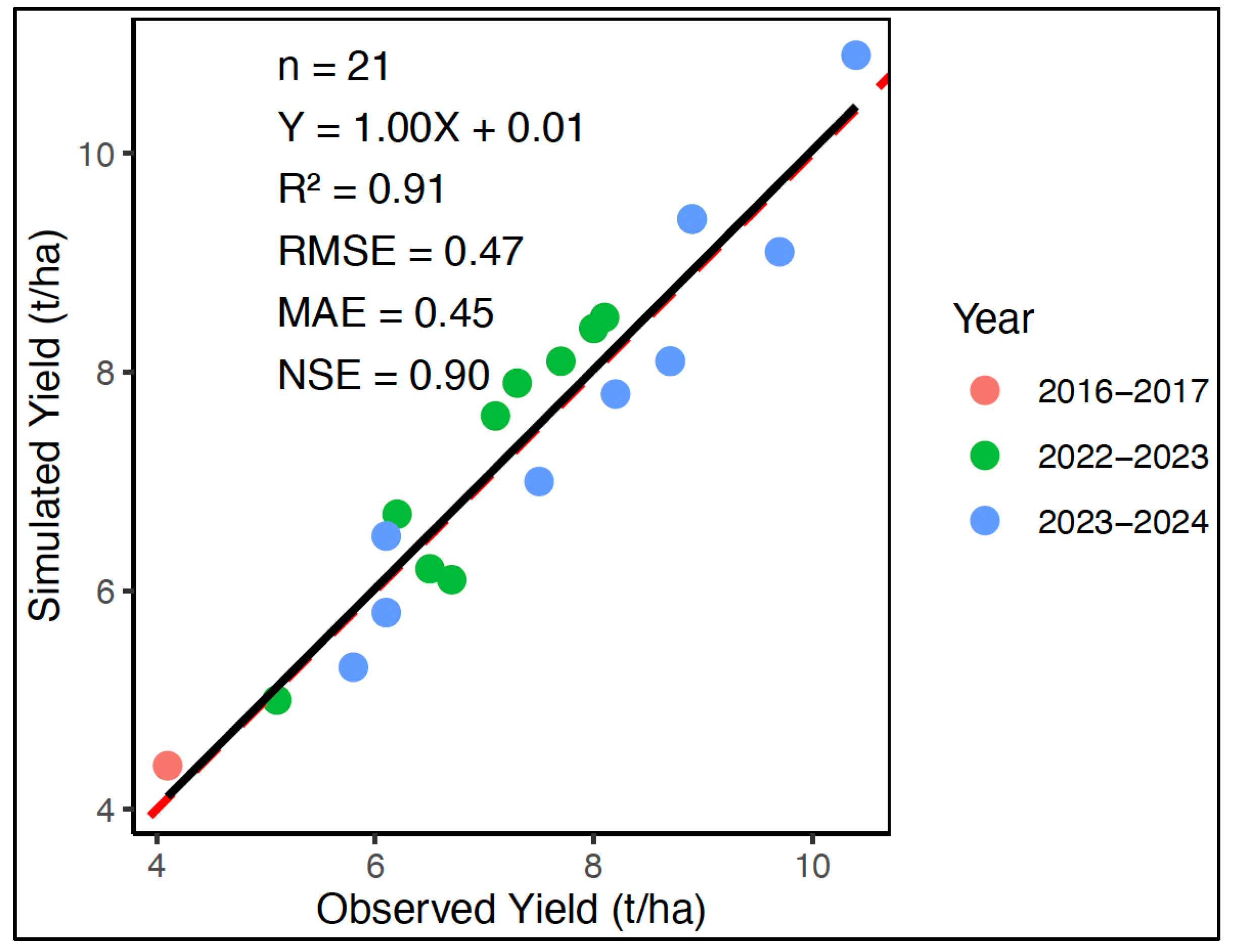
The low fertility of plinthosols is a major constraint on agricultural production, largely due to the presence of plinthite, which restricts availability of water and nutrients. This study aimed to simulate the growth and yield of grain maize on a loosened plinthosol amended with termite mound (Macrotermes falciger) material in the Lubumbashi region. A 660-hectare perimeter was established, subdivided into ten maize blocks (B1-B10) and a control block (B0), which received the same management practices as the other blocks except for subsoiling and termite-mound amendment. The APSIM model was used for simulations. The leaf area index (LAI) was estimated from Sentinel-2 imagery via Google Earth Engine, using the Simple Ratio (SR) spectral index, and integrated into APSIM alongside agro-environmental variables. Model performance was assessed using cross-validation (2/3 calibration, 1/3 validation) based on the coefficient of determination (R²), Nash–Sutcliffe efficiency (NSE), and root mean square error (RMSE). Results revealed a temporal LAI dynamic consistent with maize phenology. Simulated LAI matched observations closely (R2= 0.85-0.93; NSE = 0.50-0.77; RMSE = 0.29-0.40 m2 m-2). Grain yield was also well predicted (R2= 0.91; NSE > 0.80 ; RMSE <0.50 t ha-1). Simulated yields reproduced the observed contrast between treated and control blocks: 10.4 t ha-1 (B4, 2023–2024) versus 4.1 t ha-1 (B0). These findings highlight the usefulness of combining remote sensing and biophysical modelling to optimize soil management and improve crop productivity under limiting conditions.
Keywords:
1. Introduction
2. Materials and Methods
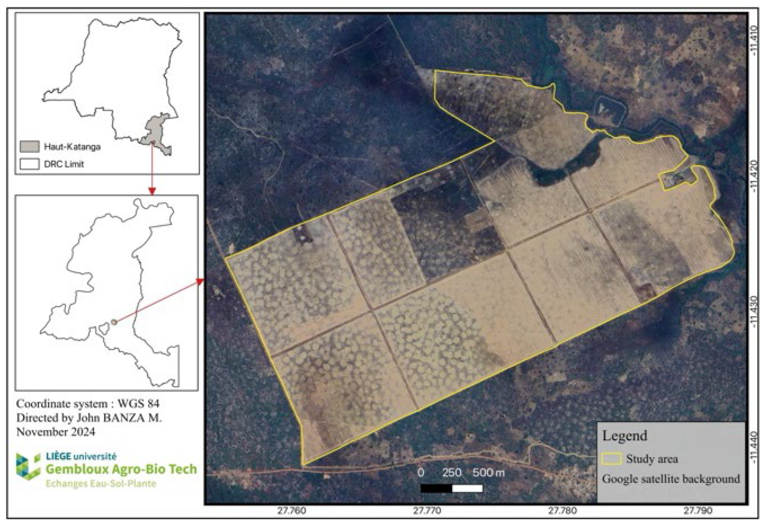
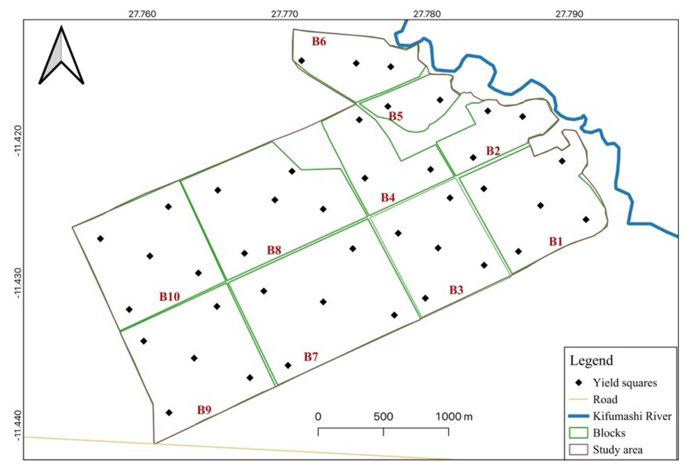
2.1. Study Sites
2.2. APSIM Model Description
2.3. Parametrization and Calibration
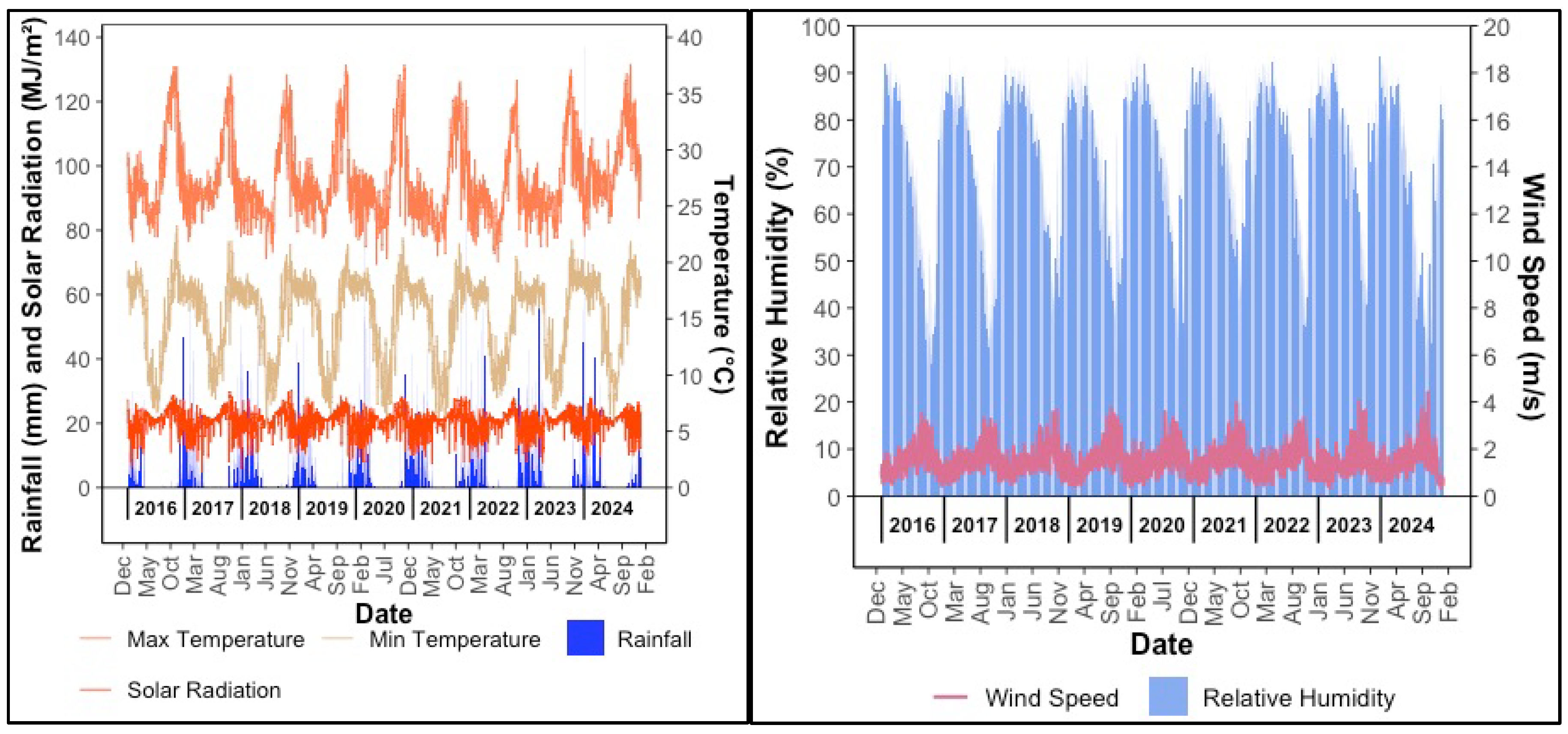
2.3.1. Climate Data
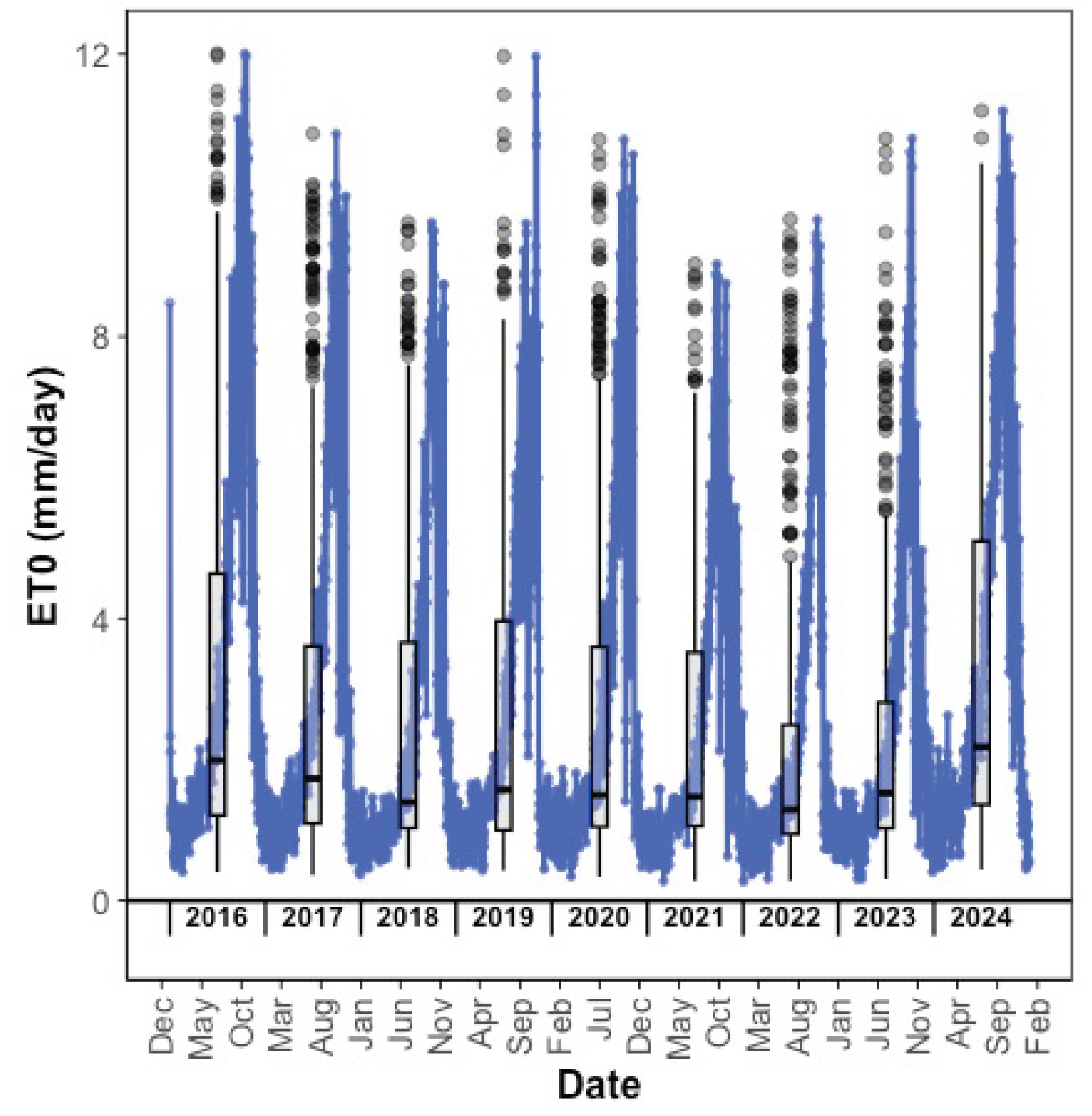
2.3.2. Reference Evapotranspiration
2.3.3. Maize Grain Yield
2.3.4. Soil Properties
2.3.5. Leaf Area Index
2.3.6. Crop Parameters and LAI Calibration
2.4. Cross-Validation
- -
- Coefficient of determination (R2), which measures the proportion of variance explained by the model (R2; Equation (3)). A value close to 1 indicates good performance.
- -
- RMSE (Root Mean Square Error), quantifying the average standard deviation between simulated and observed yields (RMSE; Equation (4)). The lower the RMSE, the more accurate the model.
- -
- NSE (Nash-Sutcliffe Efficiency), which evaluates the accuracy of the model by comparing it to the average of the observations (NSE; Equation (5)). When NSE is close to 1, the model performs well, and when it is less than 0, the model performs less well than the average of the measured yields.
- -
- MAE (Mean Absolute Error) estimates the average of the absolute differences between simulated and observed values, providing an assessment that is less sensitive to extreme errors (MAE; Equation (6)).
2.5. Simulation Runs
2.6. Data Analysis
3. Results
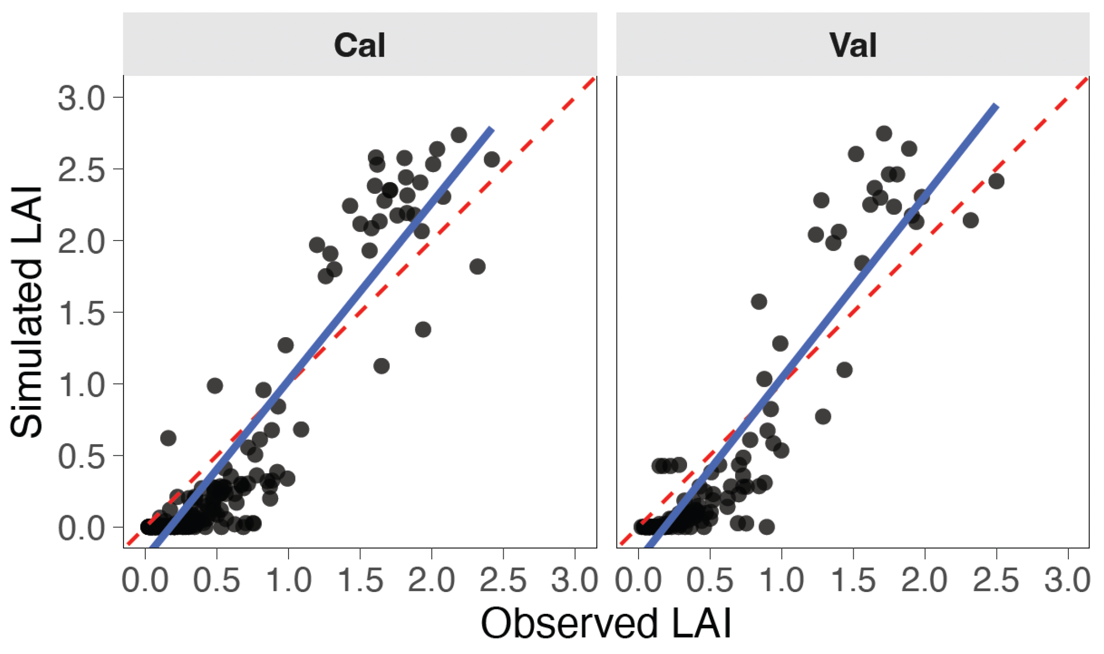
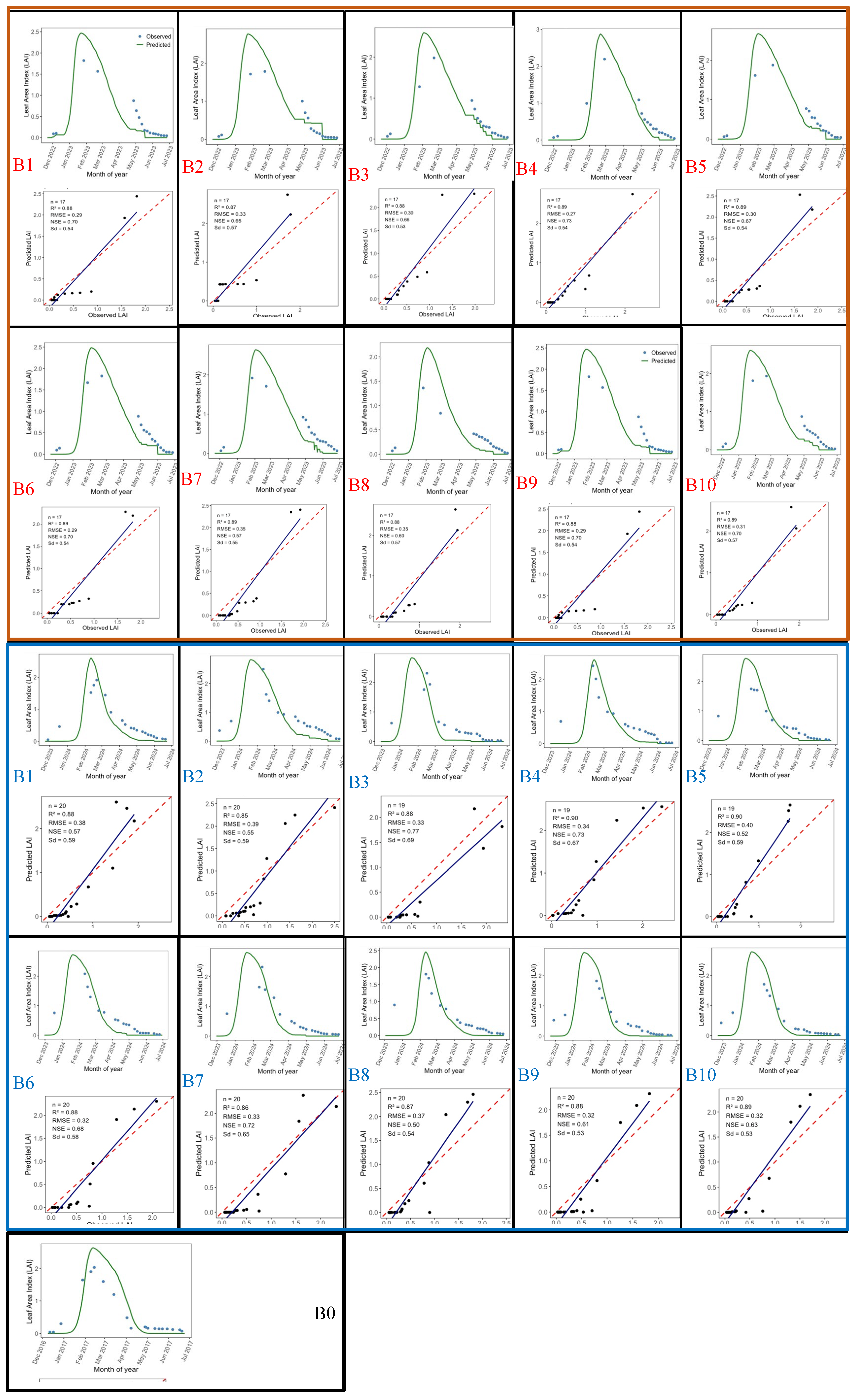
3.1. Performance of the APSIM Model for LAI Simulation
3.2. Evaluation of APSIM Model Performance in Cross-Validation of Grain Yield
3.3. Performance of the APSIM Model in Predicting Yields
4. Discussion
4.1. Evaluation of the Accuracy of LAI Derived from Sentinel-2 and Its Simulation with APSIM
4.2. Evaluation of the Performance of the APSIM Model for Simulating Maize Grain Yields
5. Conclusions
Author Contributions
Funding
Data Availability Statement
Acknowledgments
Conflicts of Interest
References
- ISS Africa RD Congo: Special Report. futures.issafrica.org, 2024. 25p, https://futures.issafrica.org/special-reports/country/drc-french.
- Mulumeoderhwa, M.F.; Maniriho, A.; Ciza, A.N.; Iyoto, E.B.; Lukeba, F.N.; Ngerizabona, S.V.; Mirindi, G.F.; Namegabe, J.L.M.; Lebailly, P. Characterization of small-scale farming as an engine of agricultural development in Mountainous South Kivu, Democratic Republic of Congo. Asian Journal of Agriculture and Rural Development 2022, 12, 123–129. [Google Scholar] [CrossRef]
- Mulume, B.S.; Dontsop, N.P.M.; Nyamugira, B.A.; Jean-Jacques, M.S.; Manyong, V.; Bamba, Z. Farmers’ credit access in the Democratic Republic of Congo: Empirical evidence from youth tomato farmers in Ruzizi Plain in South Kivu. Cogent Economics and Finance 2022, 10. [Google Scholar] [CrossRef]
- Ciza, A.N.; Mubasi, C.C.; Barhumana, R.A.; Balyahamwabo, D.K.; Mastaki, J.L.N.; Lebailly, P. Impact of non-agricultural activities on food security in Mountainous South Kivu. Tropicultura 2021, 39, 1–20. [Google Scholar] [CrossRef]
- Mushagalusa, B.A.; Nkulu, M.F.J. Potential threats to agricultural food production and farmers’ coping strategies in the Marshlands of Kabare in the Democratic Republic of Congo. Cogent Food Agric 2021, 7. [Google Scholar] [CrossRef]
- Badibanga, T.; Ulimwengu, J. Optimal investment for agricultural growth and poverty reduction in the democratic republic of congo a two-sector economic growth model. Appl Econ 2020, 52, 135–155. [Google Scholar] [CrossRef]
- Doocy, S.; Cohen, S.; Emerson, J.; Menakuntuala, J.; Rocha, J.S.; Klemm, R.; Stron, J.; Brye, L.; Funna, S.; Nzanzu, J.P.; et al. Food security and nutrition outcomes of farmer field schools in Eastern Democratic Republic of the Congo. Glob Health Sci Pract 2017, 5, 630–643. [Google Scholar] [CrossRef]
- Ochieng, J.; Ouma, E.; Birachi, E. Gender participation and decision making in crop management in Great Lakes Region of Central Africa. Gend Technol Dev 2014, 18, 341–362. [Google Scholar] [CrossRef]
- Tambwe, N.; Rudolph, M.; Greenstein, R. “Instead of Begging, i farm to feed my children”: Urban agriculture - an alternative to copper and cobalt in Lubumbashi. Africa 2011, 81, 391–412. [Google Scholar] [CrossRef]
- Mulimbi, W.; Nalley, L.; Dixon, B.; Snell, H.; Huang, Q. Factors influencing adoption of conservation agriculture in the Democratic Republic of the Congo. Journal of Agricultural and Applied Economics 2019, 51, 622–645. [Google Scholar] [CrossRef]
- Mulimbi, W.; Nalley, L.; Nayga, R.M.; Gaduh, A. Are consumers willing to pay for conservation agriculture? the case of white maize in the Democratic Republic of the Congo. Nat Resour Forum 2023, 47, 22–41. [Google Scholar] [CrossRef]
- Tabu, H.I.; Tshiabukole, J.P.K.; Kankolongo, A.M.; Lubobo, A.K.; Kimuni, L.N. Yield stability and agronomic performances of provitamin a maize (Zea mays L.) genotypes in South-East of DR Congo. Open Agric 2023, 8, 1–12. [Google Scholar] [CrossRef]
- Tabu, H.I.; Kankolongo, A.M.; Lubobo, A.K.; Kimuni, L.N. Maize yield and fall armyworm damage responses to genotype and sowing date-associated variations in weather conditions. European Journal of Agronomy 2024, 161, 127334. [Google Scholar] [CrossRef]
- Kasongo, L.M.E.; Banza, M.J.; Meta, T.M.; Mukoke, T.H.; Kanyenga, F.; Mayamba, M.G.; Mwamba, K.F.; Mazinga, K.M. Sensibilité de la culture pluviale du maïs ( zea mays l.) aux effets des épisodes secs sur un ferralsol sous amendement humifère à Lubumbashi. J Appl Biosci 2019, 140, 14316–14326. [Google Scholar]
- Kasongo, L.M.E. Evaluation des terres à multiples échelles pour la détermination de l’ impact de la gestion agricole sur la sécurité alimentaire au Katanga, R.D. Congo, Université de Gent, 2008.
- Useni, S.Y.; Ilunga, G.M.; Mulembo, T.M.; Ntumba, B.; Longanza, L.B. Amélioration de la qualité des sols acides de Lubumbashi ( Katanga, RD Congo ) par l ’ application de différents niveaux de compost de fumiers de poules. J Appl Biosci 2014, 77, 6523–6533. [Google Scholar]
- Banza, M.J.; Mwamba, K.F.; Esoma, E.B.; Meta, T.M.; Mayamba, M.G.; Kasongo, L.M.E. Evaluation de la réponse du maïs (Zea Mays L.) installé entre les haies de tithonia diversifolia à Lubumbashi, R.D. Congo. J Appl Biosci 2019, 134, 13643. [Google Scholar] [CrossRef]
- N’tambwe Nghonda, D. donné; Muteya, H.K.; Kashiki, B.K.W.N.; Sambiéni, K.R.; Malaisse, F.; Sikuzani, Y.U.; Kalenga, W.M.; Bogaert, J. Towards an inclusive approach to forest management: highlight of the perception and participation of local communities in the management of Miombo Woodlands Around Lubumbashi (Haut-Katanga, D.R. Congo). Forests 2023, 14. [Google Scholar] [CrossRef]
- Mujinya, B.B.; Adam, M.; Mees, F.; Bogaert, J.; Vranken, I.; Erens, H.; Baert, G.; Ngongo, M.; Ranst, E. Van. Spatial patterns and morphology of termite ( macrotermes falciger ) mounds in the Upper Katanga, D.R. Congo. Catena (Amst) 2014, 114, 97–106. [Google Scholar] [CrossRef]
- Adhikary, N.; Erens, H.; Weemaels, L.; Deweer, E.; Mees, F.; Mujinya, B.B.; Baert, G.; Boeckx, P.; Van Ranst, E. Effects of spreading out termite mound material on ferralsol fertility, Katanga, D.R. Congo. Commun Soil Sci Plant Anal 2016, 47, 1089–1100. [Google Scholar] [CrossRef]
- Legros, J.-P. Latérites et autres sols des régions intertropicales. Bulletin 2013, 12, 369–382. [Google Scholar]
- Sanchez, P.A. Properties and management of soils in the Tropics; JWiley.; New York, 2018; ISBN 9788578110796.
- Liu, X.N.; Hseu, Z.Y.; Chen, Z.S. Correcting the classification of plinthic ultisols on aged alluvial terraces in Taiwan. Soil Sci Plant Nutr 2020, 66, 458–468. [Google Scholar] [CrossRef]
- Yaro, D.T.; Kparmwang, T.; Raji, B.A.; Chude, V.O. The extent and properties of plinthite in a landscape at Zaria, Nigeria. International Journal of Soil Science 2006, 1, 171–183. [Google Scholar] [CrossRef]
- De Moraes, J.M.; Schuler, A.E.; Dunne, T.; Figueiredo, R. de O.; Victoria, R.L. Water storage and runoff processes in plinthic soils under forest. Hydrol. Process. 20, 2006, 20, 2509–2526. [Google Scholar] [CrossRef]
- Sarkar, A.; Bandyopadhyay, P.K. Effect of incubation duration of incorporated organics on saturated hydraulic conductivity, aggregate stability and sorptivity of alluvial and red-laterite soils. Journal of the Indian Society of Soil Science 2018, 66, 370–380. [Google Scholar] [CrossRef]
- Baumgartner, S.; Bauters, M.; Barthel, M.; Drake, T.W.; Ntaboba, L.C.; Bazirake, B.M.; Six, J.; Boeckx, P.; Van Oost, K. Stable isotope signatures of soil nitrogen on an environmental-geomorphic gradient within the Congo Basin. Soil 2021, 7, 83–94. [Google Scholar] [CrossRef]
- de Lima, S.S.; Pereira, M.G.; Pereira, R.N.; DE Pontes, R.M.; Rossi, C.Q. Termite mounds effects on soil properties in the atlantic forest biome. Rev Bras Cienc Solo 2018, 42, 1–14. [Google Scholar] [CrossRef]
- Enagbonma, B.J.; Babalola, O.O. Potentials of termite mound soil bacteria in ecosystem engineering for sustainable agriculture. Ann Microbiol 2019, 69, 211–219. [Google Scholar] [CrossRef]
- Eze, P.N.; Kokwe, A.; Eze, J.U. Advances in nanoscale study of organomineral complexes of termite mounds and associated soils : a systematic review. 2020, 2020.
- Jouquet, P.; Guilleux, N.; Ramesh, R. Influence of soil type on the properties of termite mound nests in Southern India. Applied Soil Ecology 2015, 96, 282–287. [Google Scholar] [CrossRef]
- Kaschuk, G.; Santos, J.C.P.; Almeida, J.A.; Sinhorati, D.C.; Berton, J.F. Termite activity in relation to natural grassland soil attributes. Sci Agric 2006, 63, 583–588. [Google Scholar] [CrossRef]
- Mujinya, B.B.; Mees, F.; Erens, H.; Dumon, M.; Baert, G.; Boeckx, P.; Ngongo, M.; Van Ranst, E. Clay composition and properties in termite mounds of the Lubumbashi area, D.R. Congo. Geoderma 2013, 192, 304–315. [Google Scholar] [CrossRef]
- Padonou, E.A.; Djagoun, C.A.M.S.; Akakpo, A.B.; Ahlinvi, S.; Lykke, A.M.; Schmidt, M.; Assogbadjo, A.; Sinsin, B. Role of termites in the restoration of soils and plant richness on Bowé in West Africa. Afr J Ecol 2020, 58, 828–835. [Google Scholar] [CrossRef]
- Rajeev, V.; Sanjeev, A. Impact of termite activity and its effect on soil composition. Tanzania Journal of Natural and Applied Sciences 2011, 2, 399–404. [Google Scholar]
- Seymour, C.L.; Milewski, A. V; Mills, A.J.; Joseph, G.S.; Cumming, G.S.; Cumming, D.H.M.; Mahlangu, Z. Soil biology & biochemistry do the large termite mounds of macrotermes concentrate micronutrients in addition to macronutrients in nutrient-poor African Savannas ? Soil Biol Biochem 2014, 68, 95–105. [Google Scholar] [CrossRef]
- Holzworth, D.P.; Huth, N.I.; deVoil, P.G.; Zurcher, E.J.; Herrmann, N.I.; McLean, G.; Chenu, K.; van Oosterom, E.J.; Snow, V.; Murphy, C.; et al. APSIM - evolution towards a new generation of agricultural systems simulation. Environmental Modelling and Software 2014, 62, 327–350. [Google Scholar] [CrossRef]
- Holzworth, D.; Huth, N.I.; Fainges, J.; Brown, H.; Zurcher, E.; Cichota, R.; Verrall, S.; Herrmann, N.I.; Zheng, B.; Snow, V. APSIM Next Generation: overcoming challenges in modernising a farming systems model. Environmental Modelling and Software 2018, 103, 43–51. [Google Scholar] [CrossRef]
- Harrison, M.T.; Roggero, P.P.; Zavattaro, L. Simple, efficient and robust techniques for automatic multi-objective function parameterisation: Case Studies of Local and Global Optimisation Using APSIM. Environmental Modelling and Software 2019, 117, 109–133. [Google Scholar] [CrossRef]
- Chimonyo, V.G.P.; Modi, A.T.; Mabhaudhi, T. Simulating yield and water use of a sorghum–cowpea intercrop using APSIM. Agric Water Manag 2016, 177, 317–328. [Google Scholar] [CrossRef]
- Chen, C.; Lawes, R.; Fletcher, A.; Oliver, Y.; Robertson, M.; Bell, M.; Wang, E. How well can APSIM simulate nitrogen uptake and nitrogen fixation of legume crops? Field Crops Res 2016, 187, 35–48. [Google Scholar] [CrossRef]
- Ebrahimi-Mollabashi, E.; Huth, N.I.; Holzwoth, D.P.; Ordóñez, R.A.; Hatfield, J.L.; Huber, I.; Castellano, M.J.; Archontoulis, S. V. Enhancing APSIM to simulate excessive moisture effects on root growth. Field Crops Res 2019, 236, 58–67. [Google Scholar] [CrossRef]
- Yang, X.; Li, Z.; Cui, S.; Cao, Q.; Deng, J.; Lai, X.; Shen, Y. Cropping system productivity and evapotranspiration in the semiarid loess plateau of China under future temperature and precipitation changes: An APSIM-Based analysis of rotational vs. continuous systems. Agric Water Manag 2020, 229, 105959. [Google Scholar] [CrossRef]
- Correndo, A.A.; Hefley, T.J.; Holzworth, D.P.; Ciampitti, I.A. Revisiting linear regression to test agreement in continuous predicted-observed datasets. Agric Syst 2021, 192, 103194. [Google Scholar] [CrossRef]
- Wu, Y.; He, D.; Wang, E.; Liu, X.; Huth, N.I.; Zhao, Z.; Gong, W.; Yang, F.; Wang, X.; Yong, T.; et al. Modelling soybean and maize growth and grain yield in strip intercropping systems with different row configurations. Field Crops Res 2021, 265. [Google Scholar] [CrossRef]
- Mohanty, M.; Probert, M.E.; Reddy, K.S.; Dalal, R.C.; Mishra, A.K.; Subba Rao, A.; Singh, M.; Menzies, N.W. Simulating soybean-wheat cropping system: APSIM Model parameterization and validation. Agric Ecosyst Environ 2012, 152, 68–78. [Google Scholar] [CrossRef]
- Chauhan, Y.S.; Solomon, K.F.; Rodriguez, D. Characterization of North-Eastern Australian environments using APSIM for increasing rainfed maize production. Field Crops Res 2013, 144, 245–255. [Google Scholar] [CrossRef]
- Adam, M.; MacCarthy, D.S.; Traoré, P.C.S.; Nenkam, A.; Freduah, B.S.; Ly, M.; Adiku, S.G.K. Which is more important to sorghum production systems in the Sudano-Sahelian Zone of West Africa: Climate Change or Improved Management Practices? Agric Syst 2020, 185, 102920. [Google Scholar] [CrossRef]
- Mohanty, M.; Sinha, N.K.; Somasundaram, J.; McDermid, S.S.; Patra, A.K.; Singh, M.; Dwivedi, A.K.; Reddy, K.S.; Rao, C.S.; Prabhakar, M.; et al. Soil carbon sequestration potential in a vertisol in Central India- results from a 43-year long-term experiment and APSIM Modeling. Agric Syst 2020, 184, 102906. [Google Scholar] [CrossRef]
- Li, X.; Wang, R.; Lou, F.; Ji, P.; Wang, J.; Dong, W.; Tao, P.; Zhang, Y. Subsoiling combine with layered nitrogen application optimizes root distribution and improve grain yield and N efficiency of summer maize. Agronomy 2024, 14. [Google Scholar] [CrossRef]
- He, D.; Li, G.; Luo, Z.; Wang, E. Effects of long-term fertiliser application on cropland soil carbon dynamics mediated by potential shifts in microbial carbon use efficiency. Soil Tillage Res 2025, 248. [Google Scholar] [CrossRef]
- Vogeler, I.; Carrick, S.; Cichota, R.; Lilburne, L. Estimation of soil subsurface hydraulic conductivity based on inverse modelling and soil morphology. J Hydrol (Amst) 2019, 574, 373–382. [Google Scholar] [CrossRef]
- Vogeler, I.; Carrick, S.; Lilburne, L.; Cichota, R.; Pollacco, J.; Fernández-Gálvez, J. How important is the description of soil unsaturated hydraulic conductivity values for simulating soil saturation level, drainage and pasture yield? J Hydrol (Amst) 2021, 598. [Google Scholar] [CrossRef]
- WRB-IUSS World Reference Base for Soil Resources 2014, Update 2015 International Soil Classification System for Naming Soils and Creating Legends for Soil Maps.; FAO, Ed.; Rome, 2015; ISBN 9789251083697.
- Assani, A.A. Analyse de la variabilité temporelle des précipitations (1916-1996) à lubumbashi (congo-kinshasa) en relation avec certains indicateurs de la circulation atmosphériques (Oscillation Austral) et Océaniques (El Niño/La Niña). Sécheresse 1999, 10, 245–252. [Google Scholar]
- Malaisse, F. how to live and survive in Zambezian open forest (Miombo Ecoregion). Les Presses Agronomiques de Gembloux (Belgique) 2011, 23, 91–97. [Google Scholar] [CrossRef]
- Keating, B.A.; Carberry, P.S.; Hammer, G.L.; Probert, M.E.; Robertson, M.J.; Holzworth, D.; Huth, N.I.; Hargreaves, J.N.G.; Meinke, H.; Hochman, Z.; et al. An overview of APSIM, a model designed for farming systems simulation. European Journal of Agronomy 2003, 18, 267–288. [Google Scholar] [CrossRef]
- Wilson, D.R.; Muchow, R.C.; Murgatroyd, C.J. Model analysis of temperature and solar radiation limitations to maize potential productivity in a cool climate. Field Crops Res 1995, 43, 1–18. [Google Scholar] [CrossRef]
- White, J.W.; Hoogenboom, G.; Stackhouse, P.W.; Hoell, J.M. Evaluation of NASA Satellite- and Assimilation Model-Derived Long-Term Daily Temperature Data over the Continental US. Agric For Meteorol 2008, 148, 1574–1584. [Google Scholar] [CrossRef]
- Mourtzinis, S.; Rattalino Edreira, J.I.; Conley, S.P.; Grassini, P. From grid to field: assessing quality of gridded weather data for agricultural applications. European Journal of Agronomy 2017, 82, 163–172. [Google Scholar] [CrossRef]
- Negm, A.; Minacapilli, M.; Provenzano, G. Downscaling of American National Aeronautics and Space Administration (NASA) daily air temperature in Sicily, Italy, and effects on crop reference evapotranspiration. Agric Water Manag 2018, 209, 151–162. [Google Scholar] [CrossRef]
- Khatibi, A.; Krauter, S. Validation and Performance of Satellite Meteorological Dataset Merra-2 for Solar and Wind Applications. Energies (Basel) 2021, 14. [Google Scholar] [CrossRef]
- Allen, R.G.; Pereira, L.S.; Dirk, R.; Martin, S. Crop evapotranspiration - guidelines for computing crop water requirements -; Nations, F.-F. and A.O. of the U., Ed.; 1998; ISBN 9251042195.
- Gong, L.; Xu, C. yu; Chen, D.; Halldin, S.; Chen, Y.D. Sensitivity of the penman-monteith reference evapotranspiration to key climatic variables in the Changjiang (Yangtze River) Basin. J Hydrol (Amst) 2006, 329, 620–629. [Google Scholar] [CrossRef]
- Estévez, J.; Gavilan, P.; Berengena, J. Sensitivity analysis of a penman–monteith type equation to estimate reference evapotranspiration in Southern Spain. YHDROLOGICAL PROCESSES 2009, 23, 3342–3353. [Google Scholar] [CrossRef]
- Sharifi, A.; Dinpashoh, Y. Sensitivity analysis of the penman-monteith reference crop evapotranspiration to climatic variables in Iran. Water Resources Management 2014, 28, 5465–5476. [Google Scholar] [CrossRef]
- Jerszurki, D.; de Souza, J.L.M.; Silva, L. de C.R. Sensitivity of ASCE-Penman–Monteith reference evapotranspiration under different climate types in Brazil. Clim Dyn 2019, 53, 943–956. [Google Scholar] [CrossRef]
- WRB, I.W.G. World Reference Base for Soil Resources. International Soil Classification System for Naming Soils and Creating Legends for Soil Maps; 4th ed.; International Union of Soil Sciences (IUSS): Vienna, Austria, 2022; ISBN 9798986245119. [Google Scholar]
- Saxton, K.E.; Rawls, W.J. Soil Water characteristic estimates by texture and organic matter for hydrologic solutions. Soil Science Society of America Journal 2006, 70, 1569–1578. [Google Scholar] [CrossRef]
- Turner, D.P.; Cohen, W.B.; Kennedy, R.E.; Fassnacht, K.S.; Briggs, J.M. Relationships between leaf area index and landsat tm spectral vegetation indices across three temperate zone sites. Remote Sens Environ 1999, 70, 52–68. [Google Scholar] [CrossRef]
- Gitelson, A.A.; Vina, A.; Arkebauer, T.J.; Rundquist, D.C.; Keydan, G.; Leavitt, B. Remote estimation of leaf area index and green leaf biomass in maize canopies. Geophys Res Lett 2003, 30, 4–7. [Google Scholar] [CrossRef]
- Cohrs, C.W.; Cook, R.L.; Gray, J.M.; Albaugh, T.J. Sentinel-2 leaf area index estimation for pine plantations in the Southeastern United States. Remote Sens (Basel) 2020, 12, 1–16. [Google Scholar] [CrossRef]
- White, Joseph. ; Running, S.W.; Nemani, R.; Keane, R.E.; Ryan, K.C. Measurement and remote sensing of LAI in Rocky Mountain Montane Ecosystems. Canadian Journal of Forest Research 1997, 27, 1714–1727. [Google Scholar] [CrossRef]
- Jiang, J. Leaf Area Index retrieval based on canopy reflectance and vegetation index in Eastern China. Journal of Geographical Sciences 2005, 15, 247. [Google Scholar] [CrossRef]
- Deng, F.; Chen, J.M.; Plummer, S.; Chen, M.; Pisek, J. Algorithm for global leaf area index retrieval using satellite imagery. IEEE Transactions on Geoscience and Remote Sensing 2006, 44, 2219–2229. [Google Scholar] [CrossRef]
- Blinn, C.E.; House, M.N.; Wynne, R.H.; Thomas, V.A.; Fox, T.R.; Sumnall, M. Landsat 8 based leaf area index estimation in Loblolly pine plantations. Forests 2019, 10, 1–18. [Google Scholar] [CrossRef]
- Mountrakis, G.; Im, J.; Ogole, C. Support vector machines in remote sensing: a review. ISPRS Journal of Photogrammetry and Remote Sensing 2011, 66, 247–259. [Google Scholar] [CrossRef]
- Nguy-Robertson, A.; Gitelson, A.; Peng, Y.; Viña, A.; Arkebauer, T.; Rundquist, D. Green leaf area index estimation in maize and soybean: combining vegetation indices to achieve maximal sensitivity. Agron J 2012, 104, 1336–1347. [Google Scholar] [CrossRef]
- Levitan, N.; Gross, B. Utilizing collocated crop growth model simulations to train agronomic satellite retrieval algorithms. Remote Sens (Basel) 2018, 10. [Google Scholar] [CrossRef]
- Kganyago, M.; Mhangara, P.; Alexandridis, T.; Laneve, G.; Ovakoglou, G.; Mashiyi, N. Validation of sentinel-2 leaf area index (LAI) product derived from snap toolbox and its comparison with global lai products in an African Semi-Arid agricultural landscape. Remote Sensing Letters 2020, 11, 883–892. [Google Scholar] [CrossRef]
- Harmse, C.J.; Gerber, H.; Van Niekerk, A. Evaluating several vegetation indices derived from sentinel-2 imagery for quantifying localized overgrazing in a Semi-Arid Region of South Africa. Remote Sens (Basel) 2022, 14. [Google Scholar] [CrossRef]
- D. N. Moriasi; J. G. Arnold; M. W. Van Liew; R. L. Bingner; R. D. Harmel; T. L. Veith model evaluation guidelines for systematic quantification of accuracy in watershed simulations. Trans ASABE 2007, 50, 885–900. [Google Scholar] [CrossRef]
- Song, Y.; Birch, C.; Qu, S.; Doherty, A.; Hanan, J. Analysis and modelling of the effects of water stress on maize growth and yield in Dryland conditions. Plant Prod Sci 2010, 13, 199–208. [Google Scholar] [CrossRef]
- Jin, Z.; Prasad, R.; Shriver, J.; Zhuang, Q. Crop model- and satellite imagery-based recommendation tool for variable rate N fertilizer application for the US Corn System. Precis Agric 2017, 18, 779–800. [Google Scholar] [CrossRef]
- Chauhdary, J.N.; Li, H.; Pan, X.; Zaman, M.; Anjum, S.A.; Yang, F.; Akbar, N.; Azamat, U. Modeling effects of climate change on crop phenology and yield of wheat–maize cropping system and exploring sustainable solutions. J Sci Food Agric 2025. [Google Scholar] [CrossRef]
- Santos, M.V.C.; de Carvalho, A.L.; de Souza, J.L.; da Silva, M.B.P.; Medeiros, R.P.; Junior, R.A.F.; Lyra, G.B.; Teodoro, I.; Lyra, G.B.; Lemes, M.A.M. A Modelling assessment of the maize crop growth, yield and soil water dynamics in the Northeast of Brazil. Aust J Crop Sci 2020, 14, 897–904. [Google Scholar] [CrossRef]
- Beah, A.; Kamara, A.Y.; Jibrin, J.M.; Akinseye, F.M.; Tofa, A.I.; Ademulegun, T.D. Simulation of the optimum planting windows for early and intermediate-maturing maize varieties in the Nigerian Savannas using the APSIM model. Front Sustain Food Syst 2021, 5, 1–18. [Google Scholar] [CrossRef]
- Dilla, A.; Smethurst, P.J.; Barry, K.; Parsons, D.; Denboba, M. Potential of the APSIM model to simulate impacts of shading on maize productivity. Agroforestry Systems 2018, 92, 1699–1709. [Google Scholar] [CrossRef]
- Prudnikova, E.; Savin, I.; Vindeker, G.; Grubina, P.; Shishkonakova, E.; Sharychev, D. Influence of soil background on spectral reflectance of winter wheat crop canopy. Remote Sens (Basel) 2019, 11. [Google Scholar] [CrossRef]
- Robertson, M.J.; Sakala, W.; Benson, T.; Shamudzarira, Z. Simulating response of maize to previous velvet bean (Mucuna Pruriens) crop and nitrogen fertiliser in Malawi. Field Crops Res 2005, 91, 91–105. [Google Scholar] [CrossRef]
- Peake, A.S.; Huth, N.I.; Kelly, A.M.; Bell, K.L. variation in water extraction with maize plant density and its impact on model application. Field Crops Res 2013, 146, 31–37. [Google Scholar] [CrossRef]
- Balboa, G.R.; Archontoulis, S. V.; Salvagiotti, F.; Garcia, F.O.; Stewart, W.M.; Francisco, E.; Prasad, P.V.V.; Ciampitti, I.A. A systems-level yield gap assessment of maize-soybean rotation under high- and low-management inputs in the Western US Corn Belt Using APSIM. Agric Syst 2019, 174, 145–154. [Google Scholar] [CrossRef]
- Marcillo, G.S.; Carlson, S.; Filbert, M.; Kaspar, T.; Plastina, A.; Miguez, F.E. Maize system impacts of cover crop management decisions: a simulation analysis of rye biomass response to planting populations in Iowa, U.S.A. Agric Syst 2019, 176, 102651. [Google Scholar] [CrossRef]
- Sheng, M.; Liu, J.; Zhu, A.X.; Rossiter, D.G.; Liu, H.; Liu, Z.; Zhu, L. Comparison of glue and dream for the estimation of cultivar parameters in the APSIM-Maize model. Agric For Meteorol 2019, 278, 107659. [Google Scholar] [CrossRef]
- Wang, Y.; Lv, J.; Wang, Y.; Sun, H.; Hannaford, J.; Su, Z.; Barker, L.J.; Qu, Y. Drought risk assessment of spring maize based on APSIM crop model in Liaoning Province, China. International Journal of Disaster Risk Reduction 2020, 45, 101483. [Google Scholar] [CrossRef]
- Liu, H.; Su, B.; Liu, R.; Wang, J.; Wang, T.; Lian, Y.; Lu, Z.; Yuan, X.; Song, Z.; Li, R. Conservation tillage mitigates soil organic carbon losses while maintaining maize yield stability under future climate change scenarios in northeast china: a simulation of the agricultural production systems simulator model. Agronomy 2025, 15, 1–15. [Google Scholar] [CrossRef]
- Zhao, Z.; Li, Z.; Li, Y.; Yu, L.; Gu, X.; Cai, H. Optimization of water and nitrogen measures for maize-soybean intercropping under climate change conditions based on the APSIM model in the Guanzhong Plain, China. Agric Syst 2025, 224, 104236. [Google Scholar] [CrossRef]
- Chauhdary, J.N.; Li, H.; Akbar, N.; Javaid, M.; Rizwan, M.; Akhlaq, M. Evaluating corn production under different plant spacings through integrated modeling approach and simulating its future response under climate change scenarios. Agric Water Manag 2024, 293, 108691. [Google Scholar] [CrossRef]
- Kawakita, S.; Takahashi, H.; Moriya, K. Prediction and parameter uncertainty for winter wheat phenology models depend on model and parameterization method differences. Agric For Meteorol 2020, 290, 107998. [Google Scholar] [CrossRef]
- Akhavizadegan, F.; Ansarifar, J.; Wang, L.; Huber, I.; Archontoulis, S. V. A time-dependent parameter estimation framework for crop modeling. sci rep 2021, 11, 1–15. [Google Scholar] [CrossRef]
- Fosu-Mensah, B.Y.; Manchadi, A.; Vlek, P.L.G. Impacts of climate change and climate variability on maize yield under rainfed conditions in the Sub-Humid Zone of Ghana: A Scenario Analysis Using APSIM. West African Journal of Applied Ecology 2019, 27, 108–126. [Google Scholar]
- Hoffmann, M.P.; Swanepoel, C.M.; Nelson, W.C.D.; Beukes, D.J.; van der Laan, M.; Hargreaves, J.N.G.; Rötter, R.P. Simulating medium-term effects of cropping system diversification on soil fertility and crop productivity in Southern Africa. European Journal of Agronomy 2020, 119. [Google Scholar] [CrossRef]
- Danquah, E.O.; Beletse, Y.; Stirzaker, R.; Smith, C.; Yeboah, S.; Oteng-Darko, P.; Frimpong, F.; Ennin, S.A. Monitoring and modelling analysis of maize (Zea Mays L.) yield gap in smallholder farming in Ghana. Agriculture (Switzerland) 2020, 10, 1–21. [Google Scholar] [CrossRef]
- De Azevedo, J.R.; Bueno, C.R.P. Potencialidades e limitações agrícolas de solos em assentamento de reforma agrária no município de Chapadinha-Ma. Sci Agrar 2017, 17, 1. [Google Scholar] [CrossRef]
- Dos Anjos, J.C.R.; De Andrade, A.S.; Bastos, E.A.; Da Silva, E.M. Changes in temperature of a plinthosol cultivated with sugarcane under straw levels. Comunicata Scientiae 2019, 10, 213–217. [Google Scholar] [CrossRef]
- Lohse, K.A.; Dietrich, W.E. Contrasting effects of soil development on hydrological properties and flow paths. Water Resour Res 2005, 41, 1–17. [Google Scholar] [CrossRef]
- Martins, A.P.; Glenio, G.S.; Virlei, Á.O.; Deyvid, D.C.; Leonardo, S.C. Reversibility of the hardening process of plinthite and petroplinthite in soils of the Araguaia River floodplain under different treatments. Rev Bras Cienc Solo 2018, 42, 1–13. [Google Scholar] [CrossRef]
- Rellini, I.; Trombino, L.; Carbone, C.; Firpo, M. Petroplinthite formation in a pedosedimentary sequence along a Northern Mediterranean Coast: from micromorphology to landscape evolution. J Soils Sediments 2015, 15, 1311–1328. [Google Scholar] [CrossRef]
- Wildemeersch, J.C.J.; Garba, M.; Sabiou, M.; Sleutel, S.; Cornelis, W. The effect of Water and Soil Conservation (WSC) on the soil chemical, Biological, and Physical Quality of a Plinthosol in Niger. Land Degrad Dev 2015, 26, 773–783. [Google Scholar] [CrossRef]
- Yaro, D.T.; Kparmwang, T.; Raji, B.A.; Chude, V.O. Extractable micronutrients status of soils in a plinthitic landscape at Zaria, Nigeria. Commun Soil Sci Plant Anal 2008, 39, 2484–2499. [Google Scholar] [CrossRef]
- Ramadhan, M.N.; Alfaris, M.A.A. Soil properties and maize growth as affected by subsoiling and traffic-induced compaction. IOP Conf Ser Earth Environ Sci 2023, 1225. [Google Scholar] [CrossRef]
- Wang, L.; Yu, X.; Gao, J.; Ma, D.; He, T.; Hu, S. Effect of subsoiling on the nutritional quality of grains of maize hybrids of different eras. Plants 2024, 13, 1900. [Google Scholar] [CrossRef]
- Feleke, H.G.; Savage, M.J.; Tesfaye, K. Calibration and validation of APSIM–Maize, DSSAT CERES–Maize and AquaCrop models for Ethiopian Tropical Environments. South African Journal of Plant and Soil 2021, 38, 36–51. [Google Scholar] [CrossRef]
- De Silva; Takahashi, T. ; Okada, K. Evaluation of APSIM-Wheat to simulate the response of yield and grain protein content to nitrogen application on an andosol in Japan. Plant Prod Sci 2021, 00, 1–12. [Google Scholar] [CrossRef]
- Dokoohaki, H.; Kivi, M.S.; Martinez-Feria, R.; Miguez, F.E.; Hoogenboom, G. A Comprehensive uncertainty quantification of large-scale process-based crop modeling frameworks. Environmental Research Letters 2021, 16, 84010. [Google Scholar] [CrossRef]
- Watt, L.J.; Bell, L.W.; Pembleton, K.G. A forage brassica simulation model using APSIM: Model calibration and validation across multiple environments. European Journal of Agronomy 2022, 137, 126517. [Google Scholar] [CrossRef]
- Zhang, S.; Tao, F.; Zhang, Z. Uncertainty from model structure is larger than that from model parameters in simulating rice phenology in China. European Journal of Agronomy 2017, 87, 30–39. [Google Scholar] [CrossRef]

| Maize blocks | Season 2016-2017 | Season 2022-2023 | 2023-2024 season | |||
| Sowing | harvest | sowing | harvest | sowing | harvest | |
| B1 | 11/22/22 | 06/23/23 | 11/23/23 | 06/23/24 | ||
| B2 | 11/24/22 | 06/21/23 | 11/23/23 | 06/22/24 | ||
| B3 | 11/30/22 | 06/25/23 | 11/30/23 | 06/25/24 | ||
| B4 | 12/02/22 | 06/27/23 | 11/30/23 | 06/27/24 | ||
| B5 | 12/05/22 | 06/24/23 | 12/02/23 | 06/24/24 | ||
| B6 | 12/07/22 | 06/27/23 | 12/30/23 | 06/30/24 | ||
| B7 | 12/03/22 | 06/24/23 | 11/30/23 | 05/26/24 | ||
| B8 | 12/04/22 | 06/26/23 | 12/02/23 | 06/26/24 | ||
| B9 | 11/25/22 | 06/22/23 | 11/22/23 | 06/24/24 | ||
| B10 | 11/27/22 | 06/24/23 | 11/22/23 | 06/24/24 | ||
| B0 | 12/09/16 | 06/24/17 | ||||
| Soil depth | SAT | DUL | LL | PAWC | BD |
Ksat (mm day-1) |
pH water |
TOC |
| (cm) | (V/V) | (g cm−3) | (%) | |||||
| Block 1 | ||||||||
| 0-26 | 0.491 | 0.257 | 0.157 | 0.100 | 1.35 | 7780 | 8.2 | 0.9 |
| 26-50 | 0.445 | 0.184 | 0.076 | 0.108 | 1.47 | 86.4 | 8.0 | 0.4 |
| Block 2 | ||||||||
| 0-27 | 0.423 | 0.215 | 0.159 | 0.056 | 1.53 | 51.7 | 6.9 | 0.8 |
| 27-79 | 0.434 | 0.238 | 0.195 | 0.043 | 1.50 | 664 | 5.6 | 0.2 |
| Block 3 | ||||||||
| 0-30 | 0.411 | 0.191 | 0.108 | 0.083 | 1.56 | 86.4 | 7.9 | 1.1 |
| 30-43 | 0.302 | 0.148 | 0.075 | 0.073 | 1.85 | 6130 | 6.0 | 0.6 |
| 43-80 | 0.275 | 0.144 | 0.084 | 0.060 | 1.92 | 7780 | 5.5 | 0.4 |
| Block 4 | ||||||||
| 0-20 | 0.449 | 0.232 | 0.18 | 0.052 | 1.46 | 125 | 8.4 | 1.2 |
| 20-35 | 0.551 | 0.264 | 0.191 | 0.073 | 1.19 | 126 | 8.0 | 1.8 |
| Block 5 | ||||||||
| 0-46 | 0.551 | 0.302 | 0.241 | 0.061 | 1.19 | 625 | 6.1 | 2.0 |
| 46-92 | 0.358 | 0.242 | 0.203 | 0.039 | 1.70 | 276 | 7.2 | 0.4 |
| 92-150 | 0.332 | 0.265 | 0.226 | 0.039 | 1.77 | 63.9 | 7.8 | 0.2 |
| Block 6 | ||||||||
| 0-25 | 0.483 | 0.214 | 0.137 | 0.077 | 1.37 | 333 | 5.9 | 1.2 |
| 25-132 | 0.377 | 0.194 | 0.148 | 0.046 | 1.65 | 32.9 | 6.1 | 0.2 |
| Block 7 | ||||||||
| 0-20 | 0.464 | 0.262 | 0.159 | 0.103 | 1.42 | 1210 | 8.0 | 1.2 |
| 20-30 | 0.374 | 0.184 | 0.085 | 0.099 | 1.66 | 4320 | 6.5 | 0.2 |
| 30-75 | 0.276 | 0.154 | 0.094 | 0.060 | 1.92 | 864 | 5.6 | 0.2 |
| Block 8 | ||||||||
| 0-35 | 0.449 | 0.163 | 0.098 | 0.065 | 1.46 | 44.7 | 6.0 | 0.7 |
| 35-110 | 0.343 | 0.115 | 0.062 | 0.053 | 1.74 | 400.5 | 5.8 | 0.2 |
| Block 9 | ||||||||
| 0-30 | 0.558 | 0.261 | 0.094 | 0.167 | 1.17 | 1810 | 7.1 | 1.4 |
| 30-70 | 0.449 | 0.189 | 0.085 | 0.104 | 1.46 | 892.4 | 5.3 | 0.7 |
| Block 10 | ||||||||
| 0-27 | 0.453 | 0.184 | 0.125 | 0.059 | 1.45 | 1410 | 7.5 | 2.3 |
| 27-130 | 0.389 | 0.206 | 0.155 | 0.051 | 1.62 | 767 | 7.0 | 0.3 |
| Block 0 | ||||||||
| 0-27 | 0.302 | 0.161 | 0.092 | 0.069 | 1.85 | 398.41 | 5.3 | 0.7 |
| 27-44 | 0.275 | 0.114 | 0.073 | 0.041 | 1.92 | 91.47 | 5.0 | 0.3 |
| Blocks | Horizons | Depth | Clay | Silt | Sand |
| (cm) | (%) | ||||
| B1 | Ap | 0-26 | 19.4 | 33.2 | 47.4 |
| AB | 26-50 | 18.0 | 50.7 | 31.3 | |
| B2 | Ap | 0-27 | 21.1 | 40.4 | 38.5 |
| AB | 27-79 | 28.4 | 37.7 | 33.9 | |
| B3 | Ap | 0-30 | 22.2 | 47.6 | 30.2 |
| AB | 30-43 | 20.0 | 45.2 | 34.8 | |
| Bs | 43-80 | 30.6 | 44.5 | 24.9 | |
| B4 | Ap | 0-20 | 24.1 | 57.9 | 18.0 |
| AB | 20-35 | 16.1 | 52.3 | 31.6 | |
| B5 | Ap | 0-46 | 18.6 | 56.0 | 25.4 |
| AB | 46-92 | 37.6 | 30.2 | 32.2 | |
| Bs | 92-150 | 44.0 | 27.2 | 28.8 | |
| B6 | Ap | 0-25 | 19.7 | 32.9 | 47.4 |
| AB | 25-132 | 40.2 | 28.1 | 31.7 | |
| Bs | 132-201 | 34.6 | 38.0 | 27.4 | |
| B7 | Ap | 0-20 | 20.6 | 50.5 | 28.9 |
| AB | 20-30 | 18.0 | 51.7 | 30.3 | |
| Bs | 30-75 | 24.3 | 51.3 | 24.4 | |
| B8 | Ap | 0-35 | 18.8 | 41.2 | 40.0 |
| Bcs | 35-110 | 34.1 | 45.0 | 20.9 | |
| B9 | Ap | 0-30 | 22.2 | 53.2 | 24.6 |
| Bcs1 | 30-70 | 27.8 | 49.6 | 22.6 | |
| B10 | Ap | 0-27 | 12.0 | 43.5 | 44.5 |
| Bs | 27-130 | 21.8 | 46.4 | 31.8 |
| Year | Jan | Feb | Mar | Apr | May | Jun | Jul | Aug | Sep | Oct | Nov | Dec |
| 2016 | 2 | |||||||||||
| 2017 | 2 | 2 | 2 | 2 | 3 | 4 | ||||||
| 2022 | 3 | 3 | ||||||||||
| 2023 | 2 | 2 | 2 | 7 | 7 | 3 | 3 | |||||
| 2024 | 4 | 3 | 3 | 7 | 5 | 4 | 2 | |||||
| No image | Image |
| Cultivar parameters | Description | Unit | values | Source |
| Density | Plants m-2 | 6 | Adjusted | |
| Juvenile.Target | Development time of the juvenile phase | °Cd | 170 | Adjusted |
| FloweringToGrainFilling.Target | Time required to transition from flowering to grain filling |
°Cd | 175 | Adapted |
| FlagLeafToFlowering.Target | Time from flag leaf appearance to flowering |
°Cd | 50 | Adjusted |
| GrainFilling.Target | Time required for grain filling | °Cd | 860 | Default |
| MaturityToHarvestRipe | Time from maturity to harvest | °Cd | 10 | Default |
| Photosensitive.Target. | Photoperiod sensitivity | - | 0, 12.5, 24 | Default |
| Height | Height crop | cm | 243.3 | Adjusted |
| MaximumGrainsPerCob | Maximum number of grains per ear | number | 1050 | Adjusted |
| MaximumPotentialGrainSize | Maximum theoretical grain size | g | 0.800 | Adjusted |
| Root.SpecificRootLength | Specific root length | cm/g | 100 | Default |
| Proportion of plant mortality | Proportion of plant mortality (dimensionless, between 0 and 1) |
- | 0.02 | Adapted |
| LAI | Leaf area index | m2 leaf/m2 soil | xa | Calibrated |
| Fertilizer | ||||
| N Fertilization | Urea (45% N) | kg/ha | 200 | Adapted |
| Set | LAI (m2 m-2) | Metrics | |||||
| Observed Mean | Simulated Mean | R2 | NSE | RMSE | MAE | n | |
| (m2 m-2) | |||||||
| Calibration | 0.496 | 0.394 | 0.87 | 0.71 | 0.32 | 0.25 | 220 |
| Validation | 0.513 | 0.418 | 0.85 | 0.70 | 0.35 | 0.27 | 148 |
| Overall | 0.503 | 0.404 | 0.86 | 0.67 | 0.33 | 0.26 | 368 |
| Set | Grain Yield (t ha-1) | Metrics | |||||
| Observed Mean | Simulated Mean | R2 | NSE | RMSE | MAE | n | |
| (t ha-1) | |||||||
| Calibration | 7.38 | 7.39 | 0.92 | 0.99 | 0.48 | 0.47 | 12 |
| Validation | 7.47 | 7.51 | 0.89 | 0.88 | 0.46 | 0.44 | 9 |
| Overall | 7.43 | 7.44 | 0.91 | 0.90 | 0.47 | 0.45 | 21 |
| Grain Yield (t ha-1) | ||||||
| Block | 2022-2023 | 2023-2024 | 2016-2017 | |||
| Obs | Pred | Obs | Pred | Obs | Pred | |
| B0 | (-) | (-) | (-) | (-) | 4.1 | 4.4 |
| B1 | 7.1 | 7.6 | 8.7 | 8.1 | (-) | (-) |
| B2 | 8.1 | 8.5 | 8.9 | 9.4 | (-) | (-) |
| B3 | 7.3 | 7.9 | 8.2 | 7.8 | (-) | (-) |
| B4 | 8.9 | 9.4 | 10.4 | 10.9 | (-) | (-) |
| B5 | 6.7 | 6.1 | 9.7 | 9.1 | (-) | (-) |
| B6 | 6.1 | 6.5 | 6.1 | 6.4 | (-) | (-) |
| B7 | 8.0 | 8.4 | 8.7 | 8.1 | (-) | (-) |
| B8 | 5.1 | 5.0 | 5.8 | 5.3 | (-) | (-) |
| B9 | 7.7 | 8.1 | 6.1 | 5.8 | (-) | (-) |
| B10 | 6.2 | 6.7 | 7.5 | 7.0 | (-) | (-) |
Disclaimer/Publisher’s Note: The statements, opinions and data contained in all publications are solely those of the individual author(s) and contributor(s) and not of MDPI and/or the editor(s). MDPI and/or the editor(s) disclaim responsibility for any injury to people or property resulting from any ideas, methods, instructions or products referred to in the content. |
© 2025 by the authors. Licensee MDPI, Basel, Switzerland. This article is an open access article distributed under the terms and conditions of the Creative Commons Attribution (CC BY) license (http://creativecommons.org/licenses/by/4.0/).


