
Submitted:
26 September 2025
Posted:
29 September 2025
You are already at the latest version
Abstract
The present paper aimed to develop a systematic, prescriptive and exclusively statistical problem-solving methodology that integrates scientific experimental design methods with the Six Sigma philosophy. This was used for the study and continuous improvement of a direct dyeing process for textile materials. In the first stages of the methodology, the process was systematically analyzed, the color difference was identified, using rank correlation, as the main quality requirement of the customer, and the influence of the electrolyte concentration in the dye bath on this quality characteristic was tested, using analysis of variance. In the subsequent stages, a full factorial experiment was carried out to obtain a mathematical model describing the action of the main selected influence factors on the color difference, and response surfaces and constant level curves were plotted to find the optimal settings of these influence factors. It was concluded that cotton fabric provides a more uniform chromatic reproduction, i.e. a lower color difference, compared to linen, and the electrolyte concentration of 20 g/L yielded the most stable chromatic performance for both fiber types.
Keywords:
systematic problem solving
; Six Sigma
; DMAIC
; textile dyeing
; color difference
; rank correlation
; ANOVA
; full factorial experiment
; response surface methodology
1. Introduction
In today's business landscape, characterized by fierce competition and ever-increasing customer expectations, organizations are constantly searching for ways to optimize their operations, reduce costs, and increase customer satisfaction. In this context, Six Sigma has established itself not just as a simple methodology, but as a true management philosophy, focused on continuous improvement (CI) and data-driven decision-making. Going beyond the scope of a simple set of statistical tools, Six Sigma provides an organized framework for identifying and eliminating the causes of defects and minimizing variations in business processes, being a flexible system for improving the management and performance of companies [1].
The Six Sigma strategy does not involve only the associated metrics, but also comprises an approach at both the organizational level, by establishing the belt system, and the structured implementation of changes that lead to process improvement, by adopting the systematic problem solving methodology, with the acronym DMAIC (Define–Measure–Analyze–Improve–Control). In the five successive phases, after defining the problem, the team collects data to quantify the current performance of the process and to establish a baseline, identifies the root causes of the problem, based on which they develop, test and implement solutions, these being finally consolidated as good practices to be applied further [2]. Within each of these linked stages, a wide variety of methods and techniques are used, from those specific to CI and design of experiments, to classic quality control tools and modern quality planning and management tools (Figure 1).
The DMAIC methodology has been widely adopted in various contexts, from manufacturing [3,4] and process [5] industries to services in the logistics [6] and healthcare [7] sectors, with the aim of improving processes. Thus, by applying this methodology in [8], it was possible to reduce dpmo value by 4.496 and increase the sigma value by 0.19 for a critical quality characteristic in the welding process, relating to a component of the diesel truck cabin. Kusumawardani et al. identified, using a DMAIC approach, seven types of waste within the railroad manufacturing process and classified 42.86% of activities as non-value added, pointing to substantial opportunities for improvement [9]. The case study presented in [10] demonstrated the effectiveness of solutions implemented through a Six Sigma DMAIC project, materialized by enhancing the sigma level from 3.9 to 4.45 in three months, as a result of reducing the rejection rate of rubber weather strips. Mncwango and Mdunge, in order to identify causes of low OEE in the kit packing department of a manufacturer, performed a regression analysis within DMAIC framework to model the relationship between material downtime, manpower downtime, and total downtime [11]. Rodriguez Delgadillo et al. proposed a DMAIC approach adapted for additive manufacturing to improve quality and sustainability, demonstrating the feasibility of extending the methodology to emerging technological domains [12].
Six Sigma methodologies have been applied also in various areas of textile industry for improving product quality and reducing defects. For example, Hussain et al. successfully reduced the number of major and minor fabric defects [13]. Mukhopadhyay and Ray solved the problem of weight variation in white synthetic yarn cones [14], while Das et al. succeeded in significantly reducing the percentage of reprocessed linen fabrics due to shade variation [15], by applying the DMAIC cycle.
The textile dyeing sector faces specific challenges related to quality control and standardization of technological processes, the complex issue being reflected by the large number of studies conducted in this field – Liu et al. analyzed 101 research articles from 2013 to 2022 in [16] and El Khaoudi et al. reviewed various topic studies in [17]. Some of these research are based on scientific design of experiments methods inclusively, but without these being systematically integrated into structured Six Sigma projects. Fazeli et al. modeled, using the Taguchi and full factorial design, as well as the response surface regression method, the direct dyeing of 100% cotton fabrics, for six selected dyes, and proved that the electrolyte concentration and dyeing temperature are the most important factors on the color yield [18]. In [19], Pervez et al. found a least square support vector regression model based on Taguchi’s statistical orthogonal design to predict some objective functions of the reactive cotton dyeing process, like exhaustion percentage, fixation rate, total fixation efficiency and color strength. The study carried out by Moula et al. considered dye bath pH as an independent variable and analyzed its influence on color strength, chromaticity and hue angle, as well as on color fastness of the dyed fabric to wash, to water, to alkali perspiration, to rubbing, and to light [20].
Therefore, DMAIC provides a flexible framework that allows organizations to optimize their existing processes and ensures the transition from intuitive decisions to those based on rigorous statistical analysis. However, obstacles can also be identified in the use of this methodology, such as the need for considerable resources for training implementation team members, who must specialize in a wide variety of CI and organizational management methods, as well as statistical techniques [21]. In addition, the specialized literature highlights a lack of unity of opinion regarding the importance, effectiveness and sequence of application of statistical techniques and tools within the different DMAIC stages, which may generate difficulties in creating a routine characterized by simplicity and predictability [22,23].
Consequently, the paper proposes an alternative methodology for systematic problem solving, process-oriented and based exclusively on experimental design methods, which has the advantages of defining a clear roadmap and requiring narrower skills, focused strictly on a set of statistical techniques. The new methodology was applied in an area of interest in today's industrial practice, textile dyeing.
2. Materials and Methods
The experimental research focused on the continuous improvement of textile direct dyeing process, by applying an original method of systematic problem solving, based on scientific experimental design techniques.
2.1. Textiles Direct Dyeing
Direct dyeing is, in essence, a process characterized by simplicity, based on physical and chemical phenomena, which can be divided into four stages: two stages of dye diffusion – from the bath solution to the outer surface of the fibers and, respectively, from the outside to the inside of the fibers –, between which the adsorption of the dye on the outer surface of the fiber is interspersed, so that, finally, the physico-chemical fixation of the dye takes place through hydrogen bonds, interactions of the π electrons in the dye and the material substrate, Van der Waals bonds [24,25,26].
There are several direct dyeing processes, the most widely used being the exhaustion process, which is carried out in a neutral or slightly alkaline dye bath. The typical temperature regime involves its initial regulation at 40 °C, its progressive increase to or near the boiling point (85 °C … 100 °C), the regime temperature being maintained for 30 minutes, the final cooling for dye solution exhaustion being carried out at 60 °C … 70 °C. In the vast majority of cases, after dyeing, a separate cationic dye fixation treatment is used to improve the product's wash fastness [24,25,26].
The direct dye-fabric dyeing mechanism is influenced by the intrinsic characteristics of the raw materials used, operational factors related to technology, the addition of auxiliaries, as well as the effectiveness of preliminary processes for cleaning the support material from natural (pectins, waxes, proteins) or technological (oils, glues, stains) impurities [26].
2.1.1. Raw Materials
The textile raw materials used in the research were fabrics made from natural cellulose fibers, both cotton and flax. So, experiments were carried out with a twill denim fabric type, of 100% cotton fiber content, having an areal density of (300±5) g/m2 and a high thread count per warp (thread count – 70 × 45 threads per inch), supplied by Candiani Denim (Italy).
Also, linen fabrics, having a basket weave structure, an areal density of (200±10) g/m2 and a thread count of 80 threads per inch, were tested during this study.
Direct dyes are sodium salts of sulfonic or carboxylic acids of organic compounds of the azo type. They are anionic in nature, have water solubility and high substantivity for cellulose fibers, being used due to their ease of application, relatively low costs and good migration properties [25,26].
The color recipe required to obtain the beige dye solution, based on the identification of the color of the standard provided by the customer, required the use of the dyes presented in Table 1.
2.1.2. Key Performance Indicators (KPIs) Testing
Color difference is an indicator that refers to the quantifiable variation that can occur between the desired (reference) color and the color actually obtained on the textile fiber [28]. It is one of the most important quality indicators because it can be practically determined using a spectrophotometer.
In the field of textile dyeing, the CIEHLC space is used, which is a cylindrical color space based on CIELAB, having one coordinate, luminosity L*, similar to the one in CIELAB, and the polar coordinates C* (chroma, relative saturation) and h (hue angle in the CIELAB color wheel), presented in Figure 2.
The color difference between two points of this space can be calculated with the CMC (l:c) formula [28], developed by the Colour Measurement Committee of the Society of Dyers and Colourists in England, in 1984:
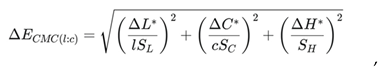
- ΔL∗, ΔC∗, ΔH∗ are the differences in luminance, chroma, and hue between the two colors;
- l and c are the adjustment factors for luminance and chroma, usually l = 2, c = 1;
- SL, SC, SH are weighting functions (tolerances) that scale the differences ΔL*, ΔC* and ΔH* according to the color reference values.
To determine the color difference, the following steps were taken [30]:
- identification of the target CIEHLC cylindrical coordinates of the color standard provided by the customer, using the spectrophotometer;
- calculating the dyeing recipe (Figure 3) by identifying the combination of three dyes, found in the database available in stock, and their share in the composition of the dye set, in order to reproduce the target color of the standard;
- preparation of samples, of the same size and shape, with uniform and defect-free surfaces for the test batch of pieces of both cotton and linen fabric;
- preparing the dyeing solution by dissolving the direct dye base, in the quantities indicated in the dyeing recipe, in an aqueous solution with neutral pH (Figure 4.a);
- introducing the samples and the dyeing solution into the cylindrical containers of the mechanical stirrer, after it has been previously brought to a temperature of 30 °C (Figure 4.b);
- raising the temperature to 40 °C and adding the neutral electrolyte (salt) in the desired concentrations to the dyeing solution for each individual sample;
- rapid increase in temperature, so as to reach the temperature indicated for each experimental test, in less than 10 minutes;
- establishing the sample time (30 minutes) from the moment the container is closed;
- extracting the samples at the end of the test time, for rinsing in two separate water baths, with detergent at 40 °C and cold water, respectively;
- squeezing and placing in an oven for drying (Figure 4.c);
- comparative reading of sample results against the color standard using a spectrophotometer and automatic calculation of the ΔE value according to the CMC (2:1) formula, used for color assessment in the field of textile materials.
The Datacolor 650™ Spectrophotometer (Figure 4.d) was used to measure the color difference. The illumination source is pulsed Xenon filtered to approximate D65, with a sphere diameter of 152 mm, wavelength range 360-700 nm, with reporting at 10 nm intervals. The spectrophotometer allows a repeatability of readings of 0.01 ΔE CIELAB maximum. Transmission sampling aperture size is 22 mm [31].
In general, if ΔE ≤ 1.0, then the color difference is imperceptible, and the sample is considered accepted. However, the acceptance limits are established according to the customer specifications.
Perspiration fastness testing simulates the exposure of a textile material to human perspiration. Artificial perspiration solutions, one alkaline and one acidic, are used to reproduce the pH conditions of human perspiration.
The testing was done according to the ISO 105-E04:2013 standard [32]. 100×40 mm strips of the test material (dyed cotton/linen) and the white/adjacent fabric were sewn together. The solutions were prepared and the pH was measured with a hand-held VARIO pH meter to ensure that the two solutions had the pH values specified in the standard (Ph 5.5 for the alkaline solution and pH 8.8 for the acidic solution). To ensure that the material samples were uniformly immersed in the solution, the Erlenmeyer flasks with test solutions were placed on magnetic stirrers (Figure 5.a) for 30 minutes. After removing the samples from the two solutions and removing the excess solution, the samples were placed between the acrylic plates of the James Heal Perspirometer Model 290 testing apparatus (Figure 5.b), and then a constant pressure of 12.5 kPa was applied (Figure 5.c). The entire assembly was placed in the HX30 model oven (Figure 5.d) at a temperature of 37±2 °C. After 4 hours the samples were removed from the oven and dried at room temperature.
For the evaluation of discoloration, the dyed cotton/linen sample was compared to an untested sample, using the Gray Scale for the Evaluation of Color Change (ISO 105-A02). A score from 5 (no change) to 1 (very large change) is given. To assess staining, the white/adjacent fabric (which has been in contact with the dyed material) is compared to the untested control material, using the Grey Scale for Stain Assessment (ISO 105-A03). A score from 5 (no staining) to 1 (very severe staining) is given.
The washing fastness test evaluates the behavior of dyed textiles in domestic washing under controlled conditions. The method simulates repeated washing and drying processes to determine the degree of color change of the dyed material and the level of staining of adjacent textiles. Sample preparation, respectively the evaluation of discoloration and staining was done similarly to those described for the perspiration test.
The test was carried out at a temperature of 40 °C in accordance with the requirements of ISO 105-C06:2010 [33]. The sample was immersed in a solution of water (grade 3), ECE Phosphate Reference Detergent (B) and sodium perborate (Figure 6.a). The test vessel, in which 6 mm diameter stainless steel balls were also inserted, was hermetically sealed and inserted into the GyroWash2 launderometer (Figure 6.b). The apparatus was set at a temperature of 40±2 °C and started for 30 minutes. After shaking, the sample was removed from the vessel (Figure 6.c), rinsed thoroughly with cold water and dried at a temperature not exceeding 60 °C.
The rubbing resistance test is performed to evaluate the ability of a dyed textile material to retain its original color during rubbing, under dry or wet conditions. The procedure consists of controlled mechanical rubbing of the sample with a standardized white cotton cloth, after which the degree of staining of the cloth is evaluated on a standardized scale from 1 to 5.
The test was performed in accordance with the ISO 105-X12:2004 standard [34], for both dry rubbing and wet drying (using distilled water), using the Crockmaster color fastness to rubbing tester (Figure 7). The friction cloth that comes into contact with the sample is fixed on the “finger”, that is, a flat-based cylinder of approximately 16 mm diameter. This is connected to a mechanical arm that performs back and forth movements along the track, while the sample remains fixed on the clamping table. The device applies a standardized vertical force of 9 N, ensuring uniform friction. The number of frictions is controlled by a counter, and a complete movement consists of a forward and backward movement of 104 mm, making 10 such movements.
2.2. New Proposed Systematic Problem Solving methodology in Six Sigma framework – DISMO
As previously mentioned, the Six Sigma strategy achieves its primary goal of reducing process variation by testing and implementing improvements through the DMAIC methodology. In each of its stages, the use of quality engineering methods and tools is recommended in the specialized literature or by practitioners [2,35,36,37,38], there being no unity of opinion regarding the importance, effectiveness and sequence of application of these techniques, which are therefore selected by users depending on the specifics of the problems addressed for solution.
On the one hand, this could be considered an advantage, supporting the creative, personalized application of the methodology, and thus creating a diversity of Six Sigma project typologies. On the other hand, it can be difficult to create, even within an organization, a routine characterized by simplicity and predictability. In addition, Six Sigma is a strategy whose metrics are statistically based, resulting logically that its implementation must be centered, with preference, on tools from this sphere, statistics. Of the methods assigned in the literature to the different DMAIC stages, not all of them meet this condition.
Therefore, within this paper, an approach to Six Sigma projects is proposed, by means of a systematic problem-solving methodology that uses scientific experimental planning methods. This results in a specific methodology, in five steps, which has the advantage of being prescriptive, based on custom, perfectly integrated into the Six Sigma philosophy. The name of the stages of the methodology, whose acronym is DISMO, as well as their content, respectively the associated objectives and methods, are described below (Figure 8).
2.2.1. Describe Interconnections Between Process Variables – D
The first phase is a preparatory stage for the use of statistical methods, facilitating a general vision of the process to be improved. It consists of a systemic analysis, SA, of the studied process, in fact a cybernetic model that presents the input and output variables, from which the influence factors, IFs, respectively the objective functions, OFs, will be selected with argumentation in the following steps of the methodology (Figure 9). Depending on the assumed objectives of the project, a detailed systemic analysis can be carried out, defining characteristic subsets for both categories of variables. Thus, the input variables can be grouped in relation to each of the structural elements of the technological transformation system and into technological operating variables, with an essential role in controlling the process subject to improvement, for achieving the desired goals. Output variables can be associated with KPIs that characterize the effectiveness, efficiency and costs of the investigated process.
An alternative tool can also be used, namely a cause-and-effect analysis, whose categories of causes, defined on the main branches of the Fishbone diagram, are among the classic, 7Ms, or customized ones. Next, it is possible to deepen the analysis by assigning scores to the causes considered more important, by each member of the work team, and ranking them according to the overall score obtained, thus carrying out a root-cause analysis, RCA.
2.2.2. Identify the Objective Function – I
In this step, the rank correlation (RC) method is applied. Usually, it is intended to order the causes that generate a result, respectively the factors that influence an objective function, based on the statistical processing of the specialists opinions.
Taking into account both its subjective nature and the fact that a pertinent analysis would require, in addition to listing all possible factors, also specifying the proposed variation ranges for them, a requisite usually not met, this methodology proposes using the method only to identify OFs of interest to clients. The method is particularly suitable for consumer goods and textile industries, for which the voice of customers is essential in defining quality characteristics, in which perception plays an important role.
The steps taken to collect, process and interpret data in order to apply the method are essentially the following [38,39]:
- Designing the survey form, by clearly listing the k selected OFs and the method of assigning ranks, distributing and completing it individually, without mutual influences, by each of the m stakeholders;
- Tabular recording of the ranks aij , associated with the characteristics Yj analyzed by each stakeholder i, in the individual forms, calculation of the sum of the ranks for each factor (by columns), Aj:
- Correction of the initial ranks aij, for stakeholders who assigned identical ranks for at least two factors, in order to establish the real position in the ordered hierarchy, tabular recalculation of the new sum of ranks for each factor, Ajc , and assignment, based on them, of the corrected global ranks, Rjc;
- Checking the adequacy of the data in the initial table with those in the corrected table, by calculating the correlation coefficient:
The new ranking is considered consistent with the initial one, if the calculated value of the rs coefficient is close to 1.
- Verifying the concordance between the points of view expressed by stakeholders, using the consensus coefficient:
where:
tj representing the number of identical ranks assigned by stakeholder i;
- Testing the statistical significance of the consensus coefficient with the chi-square criterion, since k > 7:
If the calculated value of the criterion is greater than or equal to the critical one:
then the agreement between the opinions of the stakeholders is significant, with the confidence level P = 1 – α;
- Graphical representation of the results of the ranking by a column chart, choosing as the axis of values a/Ajc, where a is a scale factor.
2.2.3. Select the Experimental Influence Factors – S
For selecting the most important IFs two methods are proposed:
- Random balance, RB, which is a supersaturated factorial experiment, carried out with the aim of ordering a number of k factors according to the effect generated on an OF, whose program matrix is constructed by randomly distributing the factor levels, provided that each level assigned to any factor appears the same number of times [39,40].
Since Two-way ANOVA will be used in the paper, only the theoretical foundations of this method will be presented below.
This procedure allows the partitioning of total variance of measured data into four parts: variances due to each factor, variance due to interaction and error variance. Thus, becomes possible, using Fisher test, to assess concurrently if the two factors and the interaction have a statistically significant effect on the investigated OF [38,40].
Considering the influence factors A and B, adjusted to a, b, levels, respectively, and the fact that each cell of the experiment contains a number of n replicates, an experimental observation can be denoted Yijk, where i = 1, …, a; j = 1, …, b; k = 1,…,n. The method involves the following steps [39,41]:
Calculating sums of squares
Total sum of squares:
- o Sum of squares for factor A:
where is the OF average value at the level i of factor A.
- o Sum of squares for factor B:
where is the OF average value at the level j of factor B.
- o Sum of squares for interaction AB:
where is the OF average value at the combination ij of factors levels.
- o Sum of squares for error (residuals):
The fundamental relation of the total variability decomposition is:
- Establishing the corresponding number of degrees of freedom:
The basic relationship of degrees of freedom:
- Calculus of the mean of squares
Mean square are calculated by dividing the sums of squares by their corresponding degrees of freedom. They represent estimates of the variance attributed to each factor.
- o Mean squares for factor A:
- o Mean squares for factor B:
- o Mean squares for interaction AB:
- o Mean squares error:
Determining Fisher's ratio
Fisher ratio for factor A:
- o
- Fisher ratio for factor B:
- o Fisher ratio for interaction AB:
- Testing the statistical significance of the influence of factors and interactions.
If the calculated Fisher ratio is greater than or equal to the critical one:
than factor A, factor B, or, respectively, interaction AB are significant with a confidence level .
Next, it is possible to continue the examination of factors influence by applying a multiple range test, which allows to compare pairs of factors levels to assess if there is a significant difference between the corresponding calculated means. To this end, an appropriate test is selected, such as Fisher LSD, Duncan, Tukey HSD, Bonferroni or Scheffé, taking into account the particular objectives and resources of the research: number of treatments, sensitivity, costs generated by false positive or false negative results.
2.2.4. Model the Investigated Process – M
Experimental mathematical modeling of a process involves identifying a relationship between an OF of interest, Y, and the essential IFs, Xj, a relationship in which the real constants are estimated through the regression coefficients bj, and the influence of the disturbing factors is included in the error associated with the experiment conducted to estimate the empirical model. It is preferred to identify the coefficients of a polynomial-form relationship, starting from a first-order polynomial, used as an exploratory or interpolation model [42,43].
The use of the modern multifactorial experimentation strategy, Box-Wilson, characterized by the slogan "all factors at every moment", involves testing the influence of factors simultaneously, at each trial [39]. Compared to the classic single-factor strategy, this strategy ensures increased certainty of results, under conditions of a lower experimental volume [38].
It is designed, in this way, a full factorial experiment, FFE, whose volume depends on the number of selected factors, k, which allows finding the regression coefficients of the polynomial model [42,43]:
For reducing the cost and time allocated to the experiment, it is also possible to design a fractional factorial experiment, which however provides lower resolutions and allows the estimation of fewer regression coefficients of interactions.
- Design and implementation of the experimental program, after identifying the customers interest on different OFs and selecting the ”vital few” IFs with their ranges of influence;
Within the experiment, each factor selected as relevant is assigned only two levels, upper and lower, coded +1 and –1, the trials consisting of all possible combinations of the levels of these independent variables. The purpose of coding the levels of IFs is to facilitate and generalize the writing of program matrices of FFEs, performed using the rule of alternating the signs of the k factors involved, at each attempt, according to the powers of 2j-1, j = 1…k.
- Model fitting by estimating regression coefficients of factors, bj, and interactions, bju:
Nonsignificant effects or interactions should be excluded from the empirical model found.
- Model adequacy check and decisions regarding further research;
In order to determine whether fitted model is adequate, a residuals analysis must be performed using Fisher test [39] or examining the residuals plot [38]. The conclusion of this analysis will be used for the substantiated establishment of subsequent decisions to be applied in the next stage of the proposed problem solving methodology.
2.2.5. Optimize the Process – O
Whether the model adequately describes reality, this will be used either for interpolation or for moving sequentially to reach an optimal region through iterative methods, like steepest ascent/descent [39]. The inadequacy of the model shows a possible identification of an optimum area, which leads to the need to resort to higher-order modeling, using central composite factorial experiments, CCFEs, or Box-Behnken designs [44].
Once a suitable mathematical model is established, the goal is to find the settings of the IFs that optimize the response. For achieving this purpose, the response surface methodology (RSM), developed by Box and Wilson for processes improvement in the chemical industry, is used [45]. The response is a quantitative continuous variable, a function that depends on the levels of the k factors, in fact real and precisely controllable values, which can be represented graphically as a surface in (k + 1) dimensions, called a response surface [45]. Practically, response surfaces are represented in the two-dimensional factorial space, choosing two quantitative factors each. Also, response surfaces can be represented, just as altitude on a map, by drawing the lines of equal response as contours [46].
Some statistical software offer the possibility to optimize a set of simultaneous OFs, by selecting the options to combine multiple objectives into a single composite score, the optimal solution being the one that maximizes this overall score, or to represent overlaid contour plots, which allow visualization of regions where multiple response variables simultaneously meet certain criteria.
3. Results
The application of the proposed DISMO problem solving methodology, namely the successive use of the statistical procedures theoretically explained in the previous paragraph for the continuous improvement of the direct dyeing process, led to the results described below.
3.1. D – Describe Interconnections Between Process Variables
The infographic presented in Figure 10 illustrates the technological flow of direct dyeing of textile materials, in which input factors (textile substrates, direct dyes, electrolytes, chemical auxiliaries, process parameters and equipment) influence the preparation, dyeing and post-treatment stages. Quality control aims to achieve KPIs that include color metrics (ΔE < 1, uniformity > 95%), as well as resistance to rubbing, washing and perspiration, according to relevant ISO standards.
The previous analysis constitutes an important support in defining the survey form used in conducting the experiment applying the rank correlation method.
3.2. I – Identify the Objective Function
As previously mentioned, in this stage the RC method was applied, with the aim of ranking a series of quality requirements that characterize the dyed textile material. So, a list of j = 9 most important presumed characteristics, Yj, was provided to i = 13 customer representatives, CRi:
- Y1 – color uniformity, meaning the absence of variations in the color characteristic parameters used in dyeing practice (hue, brightness, intensity) over the entire surface of the dyed article, which is conditioned by the migration capacity of the dyes, the dyeing speed, the temperature, the leveling auxiliaries with affinity for the fiber or dyes;
- Y2 – color fastness to household and industrial washing, i.e. the behavior of the color not to change its characteristics over time under the action of repeated washings;
- Y3 – finishing characteristics, depending on the operations performed manually on the painted product to give it a higher value or quality;
- Y4 – color fastness to perspiration, namely the stability of color characteristics over time when exposed to alkaline and acidic chemicals;
- Y5 – color difference, defined as the geometric distance between two color locations, in a color space, sensory equidistant;
- Y6 – color fastness to light, defined as the fabric ability to retain its original color when exposed both to UV radiation and natural or artificial light, by comparing its discoloration with a Blue Wool reference scale (1–8);
- Y7 – color fastness to water, meaning color stability in contact with pure water (humidity, rain, accidental washing);
- Y8 – rubbing resistance, described as the durability over time of color characteristics under repeated action of mechanical forces, tested both dry and wet;
- Y9 – delivery time, namely the deadlines established by commercial agreements for the delivery of products, after they have been subjected to the technological dyeing process.
It was formulated the requirement for these stakeholders to allocate a score for each characteristic, aij, according to their importance: 1 – to the most important, 9 – to the least important. Following the centralization of the opinions of the surveyed customer representatives, Table 2 was completed and the sums Aj of the individual ranks were calculated with formula (2), based on which the global ranks, Rj, were assigned.
It was observed that several clients’ representatives, for example CR2, CR3, CR5 and others, gave the same score to several characteristics, considering them equally important. In this situation, a correction was made to obtain the real relative position occupied by each characteristic (Table 3). Then, the data were subjected to similar processing, which resulted in the assignment of corrected global ranks, Rjc.
The correlation coefficient was calculated using relation (3): rs = 0,984 → 1. This shows that data in Table 2 and Table 3 are correlated.
The consensus coefficient was determined with formula (4), after the prior calculation of Ti and Δ j2 values with relations (5) and (6), performed in Table 2: w = 0.548. Applying relation (7) allowed us to find the value of the chi-square criterion, which was compared with its tabulated value. According to (8), since
the consensus of the clients representatives is significant, with the confidence level P = 95%.
Ordering the quality characteristics according to the importance given by customer representatives is presented in Figure 11.
Following the experiment conducted, for the quality specialists, representatives of the customers, the most important requirement regarding the quality of the products processed was the color difference, Y5, followed by the uniformity of the dyeing, Y1, these practically representing the main quality requirements of any dyeing process. Therefore, color difference was the quality characteristic on which improvement efforts were focused.
3.3. S – Select the Experimental Influence Factors
The purpose of the stage is to choose the appropriate Ifs and variation ranges for future experimental modeling of the investigated OF. Thus, in order to test the statistical significance of the influence of the neutral electrolyte (NaCl) concentration and the type of material on the color difference, ΔE, it was decided to apply bi-factorial analysis of variance, because it is more efficient than running two separate One-way ANOVAs, in the case of two materials frequently used in the textile industry – 100% cotton and linen.
So, the Two-way ANOVA was performed with a = 3 treatments (C1 – 10 g/L, C2 – 20 g/L and C3 – 30 g/L) for factor A, neutral electrolyte concentration, and b = 2 treatments (100% cotton and linen fabrics) for factor B. Each cell of the experiment was replicated n = 3 times, resulting a volume of the whole experiment N = a · b · n = 18 trials. The process duration and the regime temperature were kept constant, having the values t = 30 min and T = 95 °C, respectively. Experimental results are presented in Table 4.
The ANOVA procedure (Table 5) explained in § 2.2.3., using relations (9) … (30), decomposes the variability of color difference, ΔE, into contributions due to factors. The contribution of each factor is measured having removed the effects of all other factors.
Since p-values for both electrolyte concentration and material type are less than 0.05, these factors have a statistically significant effect on color difference, ΔE, at the 95.0% confidence level. The analysis also showed that the interaction of the factors AB is insignificant, p-value being greater than 0.05, with the same confidence level, meaning that, statistically, the effect of electrolyte concentration is similar for both materials.
The graphical representations of the estimated values of the average color difference, ΔE, and the confidence intervals (for a 95% LSD confidence level), depending on each experimental level of factors, are presented in Figure 12.a and Figure 12.b.
Figure 13 shows the interaction plot. Even though it is visually observed that the lines corresponding to the two materials are not parallel, especially between the C2 and C3 levels of electrolyte concentration, these differences in orientation shown graphically are not large enough to be confirmed as significant, so, statistically, the effect of electrolyte concentration is similar for both materials.
A multiple range test was performed for the levels of electrolyte concentration, meaning a comparison procedure to determine which means are significantly different from which others. Table 6 shows the estimated difference between each pair of means. All the 3 pairs analyzed show statistically significant differences at the 95.0% confidence level. Because the analysis involves a small number of treatments, the method selected to discriminate between means is Fisher’s least significant difference (LSD) procedure.
Since, on the one hand, for both 100 % cotton and linen fabric, at the lowest electrolyte concentration, C1, the highest averages of the color difference are obtained, and on the other hand, the contrast analysis demonstrates the existence of significant differences between the averages obtained for levels C2 and C3, in the next stage factorial experiment, a variation range between these levels was chosen, i.e. between 20 … 30 g/L.
3.4. M – Model the Investigated Process
The neutral electrolyte concentration is not the only input variable of the dyeing process that exerts a significant influence on the color difference resulting from the direct dyeing process [18,26]. In addition, these additional factors also have an important influence on other quality characteristics imposed by the customer, such as color fastness to washing, perspiration, light, etc. Therefore, in order to guide the process towards ensuring optimal values for a more comprehensive set of quality characteristics, it is necessary to model the action of several Ifs on the dependent variables of interest for the use of textile products.
Thus, to model the influence of factors on the color difference, ΔE, in the case of direct dyeing, a full factorial experiment, FFE 23, in two blocks, without randomization, was designed and conducted. This experimental strategy allows reducing the experimental volume and maximizing the estimation accuracy of a polynomial model.
Considering their importance in practice, three Ifs were selected, possibly adjustable within the analyzed process:
- neutral electrolyte concentration, C [g / l];
- dyeing temperature, T [°C];
- support material, M.
It is noted that the last of the selected factors is qualitative, being analyzed two frequently used materials in the dyeing process. For all tests, the duration of the dyeing process at the regime temperature, T, was maintained at the value t = 30 min.
The range of variation for the other two input variables – salt concentration and temperature – was chosen based on the a priori information available in the specialized literature [24,26] and the results of the preliminary experiments, presented in the previous paragraph. The physical values corresponding to the lower and upper levels for each factor are presented in Table 7. The measured values of the color difference, ΔE, obtained after conducting the experimental tests, are also shown in Table 7.
Examples of reports with results obtained when measuring the color difference, for both cotton and linen fabric, can be seen in the Figure 14, the imposed limit value of the color difference, ΔEmax = 1.2, being more demanding than that corresponding to a standard commercial quality (ΔE ≤ 1.5-2.0).
The experimental data were processed using the statistical software Statgraphics Centurion. In the first instance, the procedure performed allowed for the ranking of both main effects and interaction effects on the response function (Figure 15), using the standardized Pareto diagram.
The representation of the main effects (Figure 16) in the factors range of variation offers also the possibility of assessing the magnitude of the influence of the factors on the investigated OF, by analyzing the slopes of the lines. It is observed that the color difference is mainly influenced by the type of material – cotton or linen fabric – subjected to direct dyeing (the slope of the line is maximum), then by the electrolyte concentration, in the chosen variation interval, and least of all by the variation of the temperature, between 90°C and 100°C. The ranking of the temperature in third place is explained by the relatively small variation range chosen, located close to some optimal values recommended in the specialized literature [24,25,26].
The regression coefficients, which show the influence of the three selected factors and their interactions on the color difference, ΔE, were also calculated using the sofware (Table 8). The sign and value of each coefficient indicate the direction and amplitude of the corresponding influence.
It is observed that, as also highlighted by the Two-way ANOVA presented in the previous paragraph, increasing the neutral electrolyte concentration C, from 20 g/L to 30 g/L leads to an increase in the color difference ΔE, regardless of the type of material. Moreover, increasing the temperature, between 90°C and 100°C, also has the effect of increasing the color difference, ΔE.
Pareto diagram (Figure 14) can also be used to test the statistical significance of the regression coefficients of the model. Failure to meet the tested condition shows that the corresponding effects are insignificant, and so may be included in the free term. On the diagram (Figure 14), these effects are located below the line corresponding to a critical value. The graphic analysis highlights that, in the case of the experiment conducted, the interaction AB, between salt concentration and temperature is insignificant, while those involving the type of material are significant, but producing effects inferior to those of the factors.
Keeping only the terms of relation (31) which correspond to the significant effects, the model for coded values of the Ifs becomes:
ΔE = 0.99 + 0.156 C + 0.111 T + 0.236 M+ 0.0975 C·M + 0.045 T·M ,
The statistical significance of the influence of factors and first-order interactions on the OF can also be tested by integrating ANOVA (Table 9) into the FFE. The procedure compares the mean squares caused by the intentional variation of the factors with the random mean square, determined by measurement errors.
ANOVA (Table 9) confirms that there are 5 factor and interaction effects that are significantly different from zero at a 95% confidence level, because the critical significance threshold p-value for them is less than 0.05. The two blocks of trials, through which the experiment was replicated, were conducted in different periods. From the ANOVA it is seen that the blocks have an insignificant influence on the OF. The value of the coefficient of determination R2 = 98.106 %, shows the proportion in which model (34) explains the variation in the color difference.
The very good agreement between the measured values and those estimated with the mathematical model found can also be certified from the residuals representation in Figure 17.
3.5. O – Optimize the Process
If the relationship (34) is useful mainly from the perspective of further statistical analysis of the model and establishing the order of influence of the factors, for practical use, in the sense of estimating the color difference values using the model found, for arbitrary values of the Ifs in their range of variation, it is preferable to use a model for physical values of Ifs:
ΔE = -0.7175 – 0.01625 C + 0.00975 T – 1.10625 M+ 0.0195 C·M + 0.009 T·M ,
In both models (34) and (35), to find the ΔE values, the substitutions M = –1 for cotton, and M = +1 for linen, respectively, are used.
By means of the model (35), response surfaces of the dependent variable ΔE were represented, depending on the NaCl concentration and the bath temperature, for both investigated materials (Figure 18.a and Figure 18.b). By sectioning the response surfaces with planes parallel to that of the factors, the constant level curves for the color difference ΔE were obtained (Figure 19.a and Figure 19.b). To make these graphical representations, the physical values of the influence factors were preferred, taking into account the practical utility of such an option.
These representations can be used to identify the correlated levels of neutral electrolyte concentration and bath temperature that ensure the achievement of desired values for the color difference, which constitutes an important step towards identifying optimal areas of the process, from the point of view of the analyzed KPI.
Since the color difference is not the only KPI required by customers, the others being also influenced by the factors chosen in the experiment, color fastness tests were also performed, to perspiration, washing and rubbing, Figure 20 showing, as an example, the results obtained for a cotton sample, under dyeing conditions C = 20 g/L and T = 100 °C.
From the Figure 20 it can be seen that the discoloration of the cotton sample is imperceptible for both perspiration fastness and washing fastness at 40 °C. Also, the staining is imperceptible, for all types of adjacent material (score 5), except for Perspiration fastness in acid solution of polyester, for which a small, barely visible discoloration was obtained (score 4/5).
The material's resistance to rubbing is excellent when dry (score 5), with no color transfer occurring, while when wet rubbing a slightly lower resistance is observed (score 4), manifested through minimal color transfer.
4. Discussion
The proposed CI method assured a precise, rational roadmap, based on scientific methods for designing experiments applied throughout the five logically linked stages, each of which provided results used as input elements for the subsequent phase.
The RC method identified, as a result of the statistical ranking of stakeholders' opinions, the color difference as the most important OF among those listed in the SA. The customer representatives' choice for this quality characteristic can be explained by the fact that the textile industry must respond to demands imposed by seasonal fashion, usually with the market being dominated by one or maximum two favorite colors. As aesthetic appearance plays an essential role in attracting potential buyers, in strengthening their decision to purchase a certain product, the quality of the color is decisive. Therefore, the perception of a preferred seasonal color, but which differs from one manufacturer to another, makes each of them, once a standard has been establish, insist that the dyed materials differ from it through differences imperceptible to the human eye.
By means of ANOVA it was proved that the neutral electrolyte (NaCl) content in the dye bath significantly influences the values obtained for the color difference, ΔE, both in the case of cotton and linen at a 95% confidence level. The presence of Na⁺ ions, introduced by the neutral electrolyte into the dye bath, modifies the solubility and affinity for yarn of direct dyes, which are anions in solution, with a negative charge [24]. In addition, the electrolyte reduces the electrokinetic repulsion potential between the dye and the fibers [26]. Therefore, increasing the sodium chloride concentration, from 10 to 20 g/L, reduced the solubility of the dye and favored its more uniform adsorption and migration from solution to the fiber through the salting-out effect [48], leading to more saturated colors and a decrease in color difference. At higher concentrations, 30 g/L, agglomerations of dye and a too rapid fixation on the surface occurred, generating non-uniform deposits. According to this experiment, at a concentration of 20 g/L an optimal balance between dye affinity and fiber saturation was achieved, obtaining a minimum average value of the color difference.
Since the level of 10 g/L lead to a mean value of ΔE greater than the customer specifications, it was decides, for the next experimental stage to vary this IF between 20 g/L and 30 g/L.
The FFE showed that the color difference, ΔE, is mainly influenced by the type of material (cotton or linen fabric) subjected to direct dyeing, then by the salt concentration, within the variation range chosen and least by the temperature variation (90 – 100°C). Increasing the salt concentration from 20 g/l to 30 g/l leaded to an increase in the color difference, ΔE, regardless of the type of material. Moreover, increasing the temperature, between 90°C and 100°C, also had the effect of increasing the color difference, ΔE.
The differences between the results obtained when using cotton or linen textiles are caused by both their chemical nature and their distinct morphological structure. Although both are cellulosic, flax exhibits thicker fibers, a higher content of residual substances (pectins – 2.0% and lignin – 2.2%), a higher degree of crystallinity (70-80%), with fewer amorphous areas, lower porosity and greater structural heterogeneity [26]. These characteristics reduce the accessibility of hydroxyl groups and the swelling degree of fiber in water. As a result, the diffusion and retention of dyes are more difficult, leading to more pronounced color variations compared to cotton.
Since, following the conducted FFE, it resulted that the interactions between the type of material and each of the other two selected IFs were also statistically significant, it is proven that both the influence of electrolyte concentration and temperature on the investigated OF was different for cotton materials, respectively linen.
The solubility of direct dyes depends, in addition to the nature of the compound, on temperature conditions, which plays an essential role in the dyeing process [49]. Increasing the temperature causes improved solubility, resulting in more dye available in the bath and more intense adsorption on the fibers, with consequences in color saturation growth. Especially in the case of linen, for temperatures close to boiling, adsorption may be uneven, caused by structural differences in porosity, producing variations in color tone. At the same time, higher temperature accelerates diffusion and favors the fixation of a greater amount of dye in the fiber, generating changes in hue or intensity. Moreover, a higher temperature positively influences the affinity and, implicitly, the migration of dye molecules in the fibers, increasing ΔE.
In addition to the previous, generally valid influences, some particularities can also be identified for the color beige. This color was obtained by mixing three direct dyes, which react differently to increasing temperature (only CI Direct Orange 39 is part of class A, being self-leveling, the other two belonging to class B), generating an imbalance between the components and, ultimately, a difference in hue, which means a higher ΔE. Besides, in light colors, the differences in adsorption on the fiber become more obvious than in dark colors, in the case of linen, where the fiber is more inhomogeneous, the phenomenon being accentuated. So, increasing temperature leaded to an increase in the color difference, by changing not only the intensity, but also the tone (the deviation from the desired shade), due to the different behavior of the coloring components.
As can be seen from the relationships (34), (35) and Figure 18.a and Figure 18.b., the optimal settings for FI levels, which ensures the lowest value for ΔE, are C = 20 g/L and T = 90 °C, for both cotton and linen fabrics. The importance of Figure 19.a and Figure 19.b lies in the possibility offered to find combinations of FIs that improve other KPIs imposed by customers, while simultaneously obtaining a color difference lower than a specified limit value. Qualitative information known from previous expertise can be used for this purpose. Thus, it is known that higher electrolyte concentration values lead to a decrease in wash fastness and color degradation of the dyed material, so they should be avoided. Also, higher temperature values, from the range that ensures a color difference accepted by the customer, will be preferred, because they determine a superior wash fastness, by increasing the affinity of the dye for the textile fiber. If premium quality of textiles dyed in a light color (beige) is desired, the customer imposing, for example, in order to reduce the risk of perceptible color differences, limit values ΔE ≤ 0.7 for cotton and, respectively, ΔE ≤ 1.0 for linen, the previously mentioned constant level curves can be used. Thus, from Figure 19.a, the maximum possible temperature for cotton, T = 95 °C, is identified at the intersection of the curve ΔE = 0.7 with the ordinate axis, which corresponds to a minimum concentration value C = 20 g/L. Similarly, intersecting the ordinate axis with the curve ΔE = 1.0 in Figure 19.b, for linen, the FIs settings, C = 20 g/L and T = 96 °C, are found.
In fact, the FIs selected in the final experimental work have a synergistic action: the neutral electrolyte modifies the ionic balance and solubility, the temperature regulates the energy of the system, while the intrinsic properties of the material determine the adsorption and retention capacities. Thus, the color difference is a result of the complex action of these FIs, for each material-dye pair being necessary to identify the salt concentration and temperature that ensures the desired color.
5. Conclusions
The research carried out by means of DISMO, the new systematic solving problem methodology proposed, allowed the achievement of mathematical modeling of the dyeing process of cotton and linen textile supports, for beige color. Models found, together with the related constant level curves, allow for scientifically substantiated decisions to be made, with the ultimate goal of standardizing the direct dyeing process.
Repeating the proposed problem solving method for other materials or colors, and possibly for other quality characteristics, facilitates the establishment of a knowledge base, which can be useful for promptly resolving customer requirements.
Author Contributions
Conceptualization, D.V.G.; methodology, D.V.G. and R.A.U.; software, D.V.G. and A.A.H..; validation, D.V.G., R.A.U. and A.A.H.; formal analysis, A.A.H..; investigation, R.A.U.; resources, R.A.U.; data curation, D.V.G.; writing—original draft preparation, D.V.G. and R.A.U.; writing—review and editing, D.V.G. and A.A.H..; visualization, A.A.H.; supervision, A.A.H.; project administration, R.A.U. All authors have read and agreed to the published version of the manuscript.
Funding
This research received no external funding.
Data Availability Statement
The original contributions presented in this study are included in the article. Further inquiries can be directed to the corresponding author.
Acknowledgments
The authors would like to express their gratitude to Intercolor SRL, Timisoara, for facilitating the experimental research carried out.
Conflicts of Interest
The authors declare no conflicts of interest.
Abbreviations
The following abbreviations are used in this manuscript:
| CI | Continuous Improvement |
| DMAIC | Define–Measure–Analyze–Improve–Control |
| OEE | Overall Equipment Effectiveness |
| KPI | Key Performance Indicator |
| DISMO | Describe–Identify–Select–Model–Optimize |
| OF | Objective Function |
| IF | Influence Factor |
| SA | Systemic Analysis |
| RCA | Root-Cause Analysis |
| RC | Rank Correlation |
| ANOVA | Analysis of Variance |
| RB | Random Balance |
| FFE | Full Factorial Experiment |
| CCFE | Central Composite Factorial Experiment |
| RSM | Response Surface Methodology |
References
- Pande, P.S.; Neuman, R.P.; Cavanagh, R.R. Six Sigma; All: Bucharest, Romania, 2008; p. 25.
- George, M.L.; Rowlands, D.; Price, M.; Maxey, J. Using DMAIC to Improve, Speed, Quality, and Cost. In The Lean Six Sigma Pocket Toolbox; McGraw Hill: New York, USA, 2005; pp. 1–26.
- Gaikwad, L.M.; Sunnapwar, V.K.; Teli, S.N.; Parab, A.B. Application of DMAIC and SPC to Improve Operational Performance of Manufacturing Industry: A Case Study. J. Inst. Eng. India Ser. C 2017, 100, pp. 229–238. [CrossRef]
- Jou, Y.-T.; Silitonga, R.M.; Lin, M.-C.; Sukwadi, R.; Rivaldo, J. Application of Six Sigma Methodology in an Automotive Manufacturing Company: A Case Study. Sustainability 2022, 14, 14497. [CrossRef]
- Hung, H. C.; Sung, M. H. Applying six sigma to manufacturing processes in the food industry to reduce quality cost. Scientific Research and Essays 2015, 6(3), pp. 580-591. [CrossRef]
- Adeodu, A.; Maladzhi, R.; Kana-Kana Katumba, M.G., Daniyan, I. Development of an improvement framework for warehouse processes using lean six sigma (DMAIC) approach. A case of third party logistics (3PL) services. Heliyon 2023, 9(4), e14621.
- Monday, LM. Define, Measure, Analyze, Improve, Control (DMAIC) Methodology as a Roadmap in Quality Improvement. Glob J Qual Saf Healthc. 2022, 5(2), pp. 44-46. [CrossRef]
- Imansuri, F.; Chayatunnufus, T.; Safril, Sumasto, F.; Purwojatmiko, B.H.; Salati, D. Reducing Defects using DMAIC Methodology in an Automotive Industry. Spektrum Industri 2024, 22(1), pp. 1-13. [CrossRef]
- Kusumawardani, R.; Ana; Singgih, M.L. Achieving Manufacturing Excellence Using Lean DMAIC. Eng. Proc. 2025, 84, 7. [CrossRef]
- Mittal, A.; Gupta, P.; Kumar, V.; Al Owad, A.; Mahlawat, S.; Singh, S. The performance improvement analysis using Six Sigma DMAIC methodology: A case study on Indian manufacturing company. Heliyon. 2023, 9(3). [CrossRef]
- Mncwango, B.; Mdunge, Z.L. Unraveling the Root Causes of Low Overall Equipment Effectiveness in the Kit Packing Department: A Define–Measure–Analyze–Improve–Control Approach. Processes 2025, 13, 757. [CrossRef]
- Rodriguez Delgadillo, R.; Medini, K.; Wuest, T. A DMAIC Framework to Improve Quality and Sustainability in Additive Manufacturing—A Case Study. Sustainability 2022, 14, 581. [CrossRef]
- Hussain, T.; Jamshaid, H.; Sohail, A. Reducing defects in textile weaving by applying Six Sigma methodology: A case study. Int. J. Six Sigma and Competitive Advantage 2014; 8(2), pp. 95–104. [CrossRef]
- Mukhopadhyay, A. R.; Ray, S. Reduction of Yarn Packing Defects Using Six Sigma Methods: A Case Study. Quality Engineering 2006, 18(2), pp. 189–206. [CrossRef]
- Das, P.; Roy, S.; Antony, J. An Application of Six Sigma Methodology to Reduce lot-to-lot Shade Variation of Linen Fabrics. Journal of Industrial Textiles 2007, 36(3), pp. 227-251. [CrossRef]
- Liu, S.; Liu, Y.K.; Lo, K.C.; Kan, C. Intelligent techniques and optimization algorithms in textile colour management: a systematic review of applications and prediction accuracy. Fashion and Textiles 2024, 11(13). [CrossRef]
- El Khaoudi, M.; El Bakkali, M.; Messnaoui, R.; Cherkaoui, O.; Soulhi A. Literature review on artificial intelligence in dyeing and finishing processes. Data and Metadata 2024; 3:360. [CrossRef]
- Fazeli, F.; Tavanai, H.; Hamadani, A.Z. Application of Taguchi and Full Factorial Experimental Design to Model the Color Yield of Cotton Fabric Dyed with Six Selected Direct Dyes. Journal of Engineered Fibers and Fabrics 2012, 7(3), pp. 34–42.
- Pervez, M.N.; Yeo, W.S.; Lin, L.; Xiong, X.; Naddeo, V.; Cai. Y. Optimization and prediction of the cotton fabric dyeing process using Taguchi design-integrated machine learning approach. Sci Rep. 2023, 13:12363, pp. 1–14. [CrossRef]
- Moula, G.; Hosen, D.; Siddiquee, A.B.; Momin, A.; Kaisar, Z.; Al Mamun, A.; Islam, A. Effect of dye bath pH in dyeing of cotton knitted fabric with reactive dye (Remazol Yellow RR) in exhaust method: impact on color strength, chromatic values and fastness properties. Heliyon 2022, 8, e11246. [CrossRef]
- Antony, J. Six Sigma vs Lean: Some perspectives from leading academics and practitioners. Int. J. Productivity and Performance Management 2011, 60 (2), pp. 185-190. [CrossRef]
- Chakravorty, S.S. Six Sigma programs: An implementation model. Int. J. Production Economics 2009, 119, pp. 1–16. [CrossRef]
- Kumar, M.; Antony, J.; Tiwari, M.K. Six Sigma implementation framework for SMEs – a roadmap to manage and sustain the change. Int. J. Production Research 2011, 49(18), pp. 5449-5467. [CrossRef]
- Burkinshaw, S.M. Physico-chemical aspects of textile coloration; John Wiley & Sons: New York, USA, 2015; pp. 153–200. [CrossRef]
- Kiron, M. Classification, Application and Aftertreatment of Direct Dyes. Available online: https://textilelearner.net/direct-dye-classification/ (accessed on 07.12.2024).
- Dobrovăț, M.; Grigoriu, A.; Alexandrescu, I.; Bidalach, R.; Cernat, M.; Muscă, M.; Nagy, G.; Petraru, M.; Popescu, M; Îndrumar teoretic și practic pentru vopsirea materialelor textile. CERTEX: Bucharest, Romania, 1994; pp 29–40.
- Archive for the 'Direct Dyes' Category. Available online: https://www.worlddyevariety.com/direct-dyes (accessed on 07.12.2024).
- Kuehni, R. G. Quality Control: Color Difference Perception and Calculation. In Color Vision and Technology. AATCC, USA, 2008; pp. 200–222.
- Nguyen, T.A. Effect of Biodegradable and Metallic Mordants on Dyeing Cotton Fabric with Spent Coffee Grounds. In Proceedings of the 6th International Conference on Green Technology and Sustainable Development (GTSD), Nha Trang, Vietnam, July 2022.
- ISO 105-J03:2009 Textiles -- Tests for colour fastness -- Part J03: Calculation of colour differences.
- Datacolor 650™ User Guide. Available online: https://www.datacolor.com/wp-content/uploads/2022/04/Datacolor-650-600-400-Users-Guide-4230-0395M-Rev1.pdf (accessed on 07.12.2024).
- ISO 105-E04:2013 Textiles -- Tests for colour fastness -- Part E04: Colour fastness to perspiration.
- ISO 105-C06:2010 Textiles -- Tests for colour fastness -- Part C06: Colour fastness to domestic and commercial laundering.
- ISO 105-X12:2004 Textiles -- Tests for colour fastness -- Part X12: Colour fastness to rubbing.
- Lean Six Sigma DMAIC Process Explained with Example and Case Study. Available online: https://www.reddit.com/r/OperationExcellence/comments/ov7hsx/lean_six_sigma_dmaic_process_explained_with/ (accessed on 04.09.2020).
- Šibalija, T.V.; Majstorović, V.D. Integrating Lean with/within Six Sigma. Int. J. ’’Total Quality Management & Excellence’’ 2010, 38x(4).
- Six Sigma tools for DMAIC Phases. Available online: https://www.sprintzeal.com/blog/dmaic-tools (accessed on 04.09.2020).
- Gubencu, D.V. Îmbunătățirea continuă a proceselor tehnologice; Politehnica: Timișoara, Romania, 2023; pp. 154–173, pp. 232–246, pp. 355–382.
- Taloi, D. Optimizarea proceselor tehnologice, 2nd ed.; Academiei RSR: Bucharest, Romania, 1987; pp. 101–129, pp. 170–179.
- Hinkelmann, K.; Kempthorne, O. Design and Analysis of Experiments, Volume 2. Advanced Experimental Design; John Wiley & Sons: New Jersey, USA, 2005; pp. 241–278, pp. 596–607.
- Berenson, M.L.; Levine, D.M. The Analysis of Variance. In Basic Statistics for Business Concepts and Applications, 4th ed.; Prentice-Hall: New Jersey, USA, 1989; pp. 478–492.
- Montgomery, D.C. Design and Analysis of Experiments, 5th ed.; John Wiley and Sons: New York, USA, 2001; pp. 218-276.
- Anthony, J. Design of Experiments for Engineers and Scientists, 2nd ed.; Elsevier: London, GB, 2014; pp. 95–124.
- Hinkelmann, K.; Kempthorne, O. Response Surface Design. In Design and Analysis of Experiments, Volume 1. Introduction to Experimental Design, 2nd ed.; John Wiley & Sons: New Jersey, USA, 2008; pp. 497–531.
- Dean, A.; Voss, B. Response Surface Methodology. In Design and Analysis of Experiments; Springer: New York, USA, 1999; pp. 547–592.
- John, P.W.M. Response Surfaces. In Statistical Design and Analysis of Experiments; Society for Industrial and Applied Mathematics: Philadelphia, USA, 1998; pp. 193–219.
- F Distribution Probability Calculator. Available online: https://stattrek.com/online-calculator/f-distribution (accessed on 04.04.2025).
- Wolela, A.D. Effect and Role of Salt in Cellulosic Fabric Dyeing. Adv. Res. Text. Eng. 2021, 6(1): 1061.
- Luan, F.; Xuan Xu, X.; Liu, H.; Dias Soeiro Cordeiro, M.N. Review of quantitative structure-activity/property relationship studies of dyes: recent advances and perspectives. Color. Technol. 2013, 129, pp. 173–186. [CrossRef]
Figure 1.
Conceptual hierarchy of CI strategies, methods, techniques and tools.
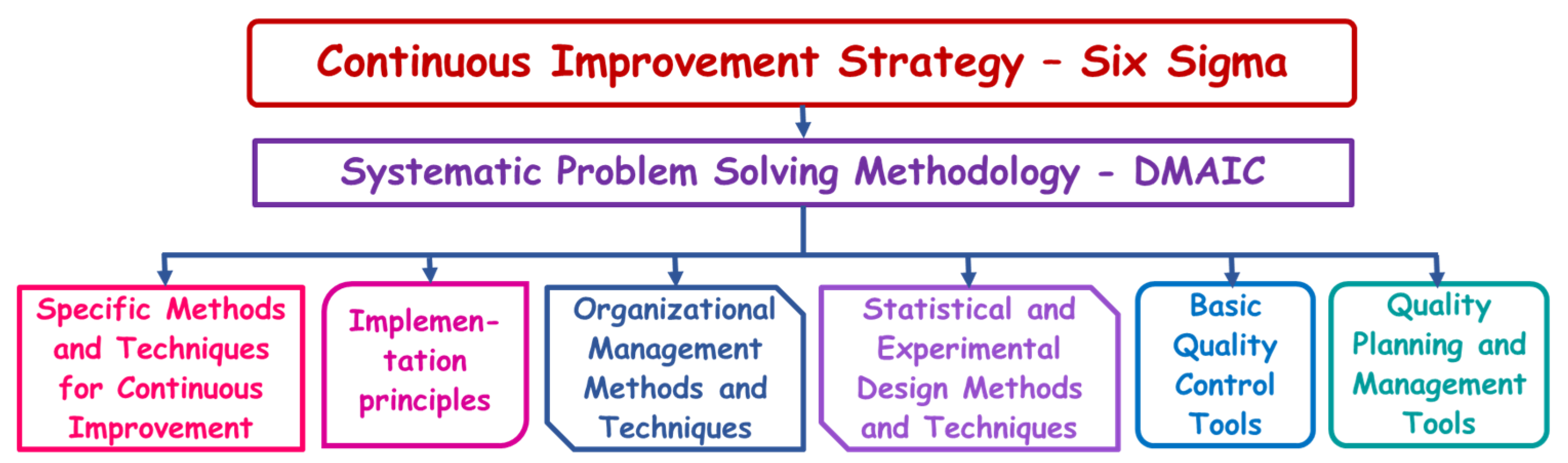
Figure 2.
Explanation for the color difference [29].
Figure 2.
Explanation for the color difference [29].
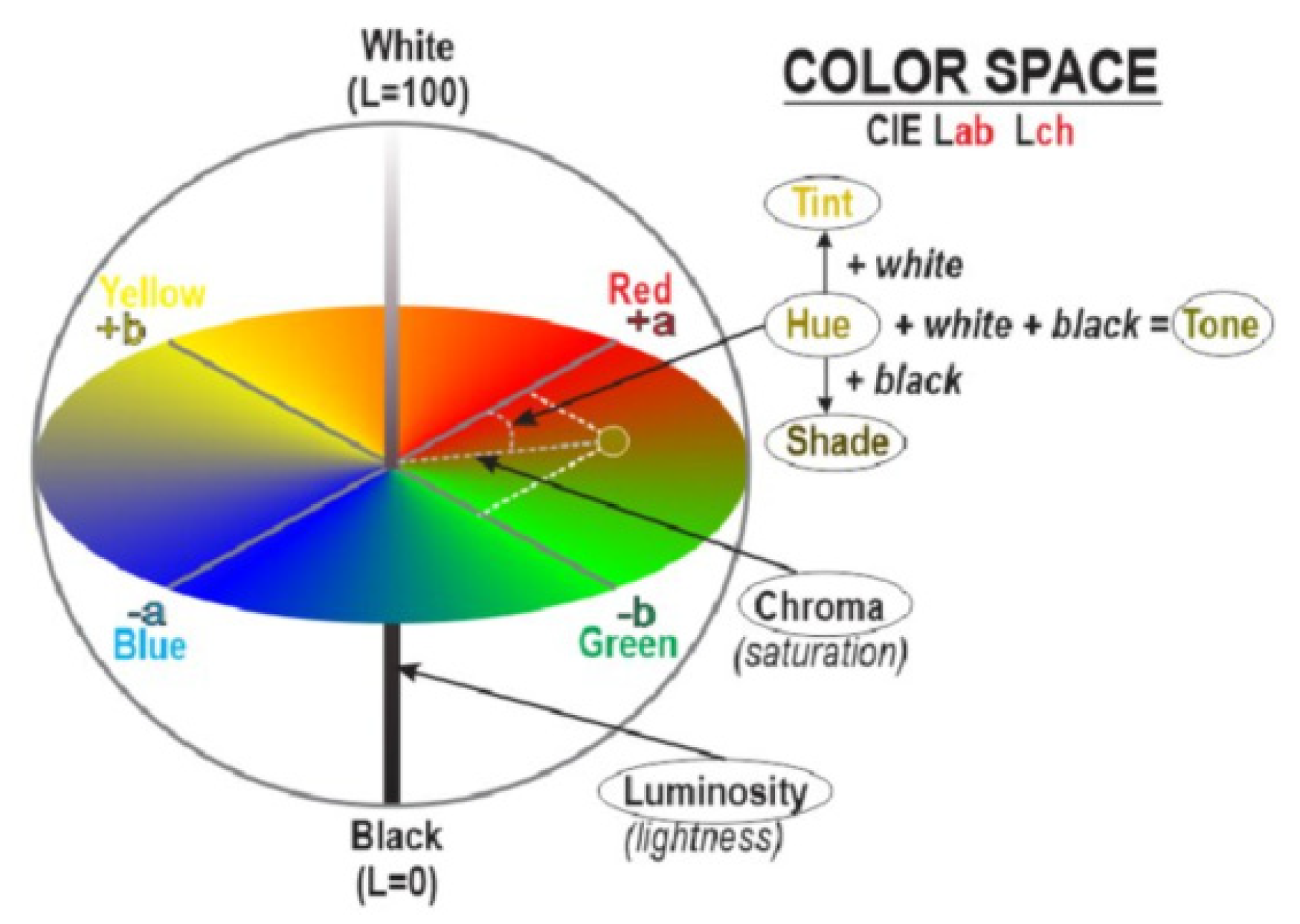
Figure 3.
Successive corrections of the color recipe.
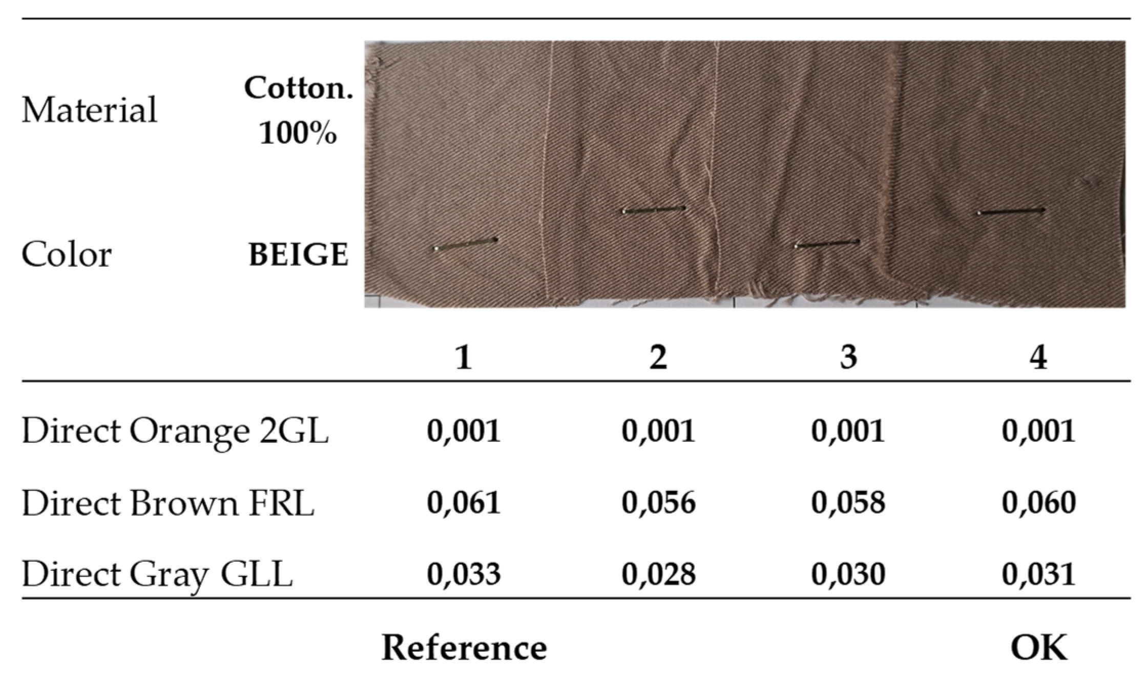
Figure 4.
Color difference, ΔE, testing: (a) preparation of the solution; (b) mechanical stirrer; (c) sample drying oven; (d) Datacolor 650™ Spectrophotometer.
Figure 4.
Color difference, ΔE, testing: (a) preparation of the solution; (b) mechanical stirrer; (c) sample drying oven; (d) Datacolor 650™ Spectrophotometer.
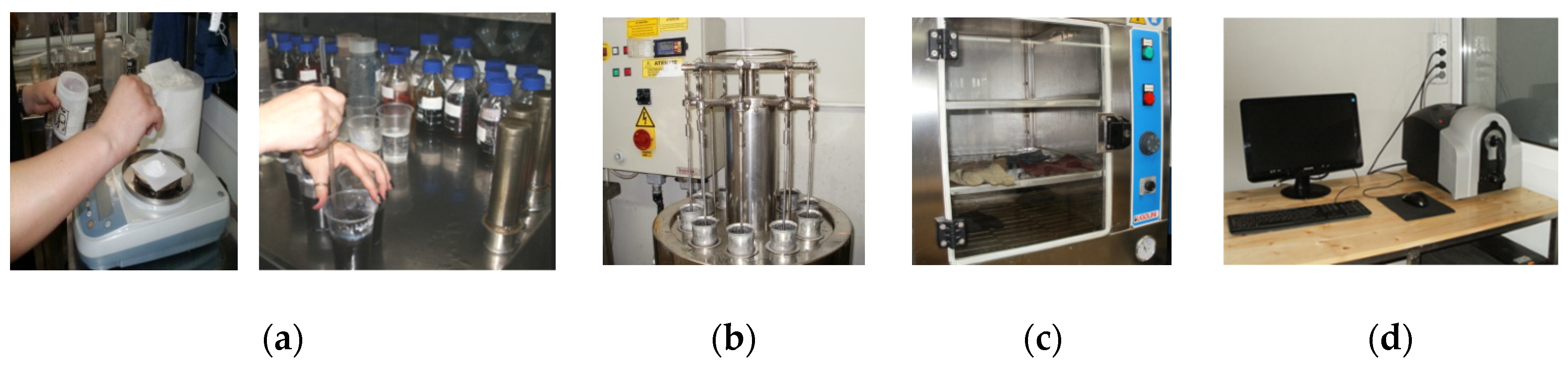
Figure 5.
Perspiration fastness testing: (a) impregnation of samples; (b) sample placement; (c) applying pressure; (d) HX30 model oven.
Figure 5.
Perspiration fastness testing: (a) impregnation of samples; (b) sample placement; (c) applying pressure; (d) HX30 model oven.
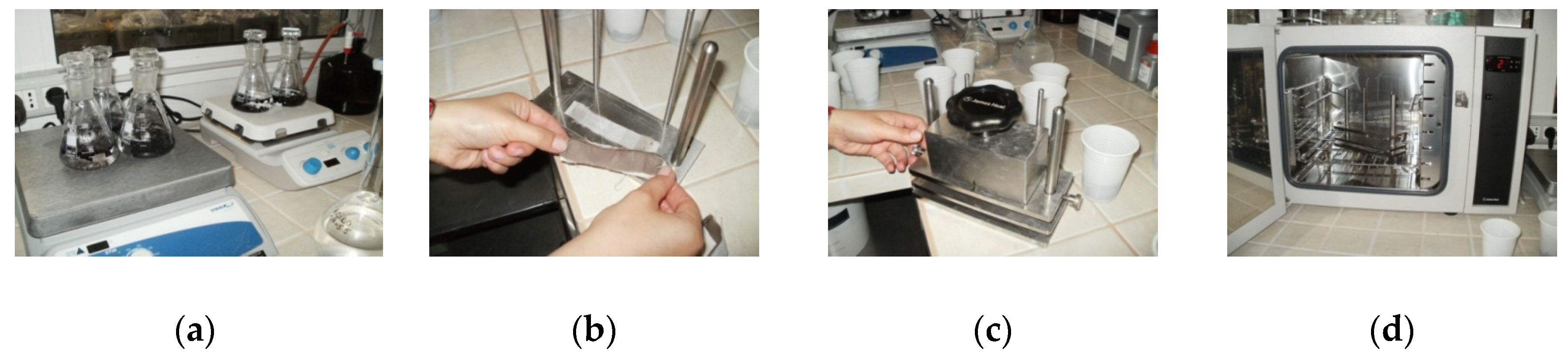
Figure 6.
Washing fastness testing: (a) immersion of samples in solution; (b) launderometer; (c) samples after washing.
Figure 6.
Washing fastness testing: (a) immersion of samples in solution; (b) launderometer; (c) samples after washing.
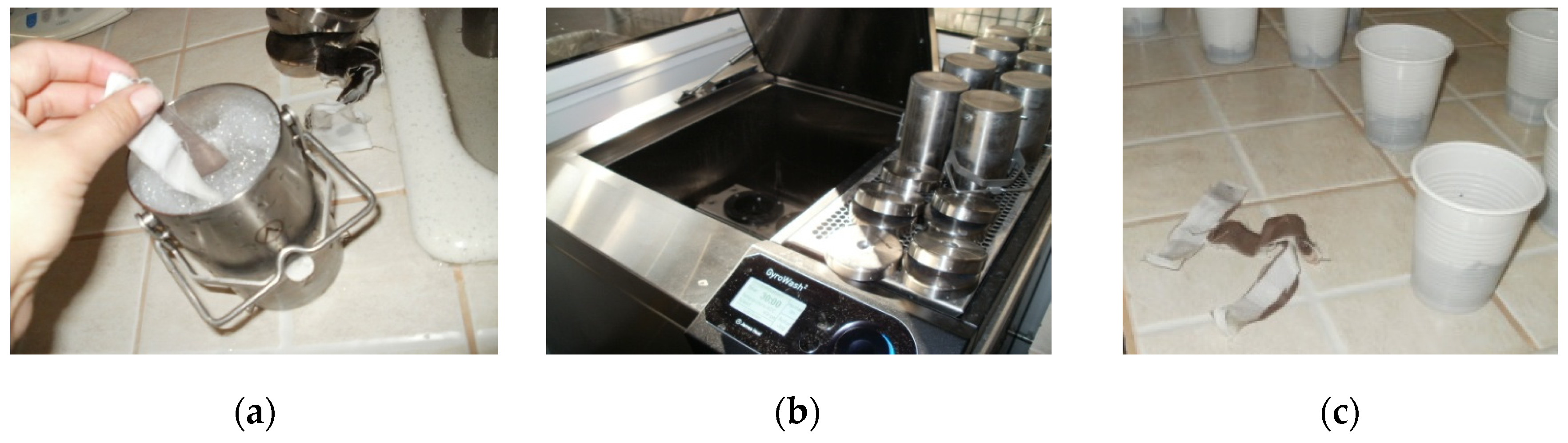
Figure 7.
Wet rub resistance testing with Crockmaster: (a) standardized white cotton cloth; (b) fixing the friction cloth; (c) setting test parameters; (d) results report.
Figure 7.
Wet rub resistance testing with Crockmaster: (a) standardized white cotton cloth; (b) fixing the friction cloth; (c) setting test parameters; (d) results report.
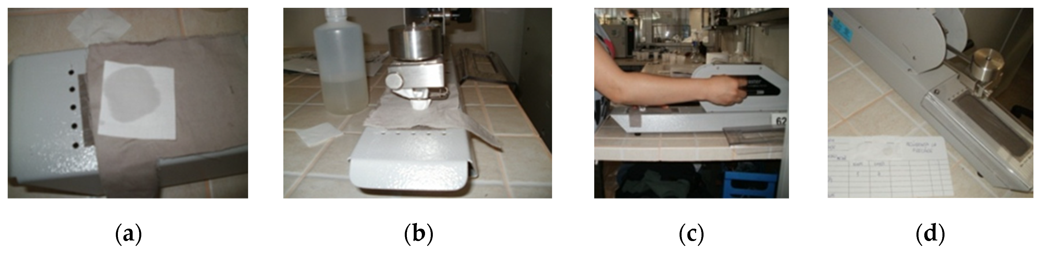
Figure 8.
Proposed systematic problem solving method – DISMO.
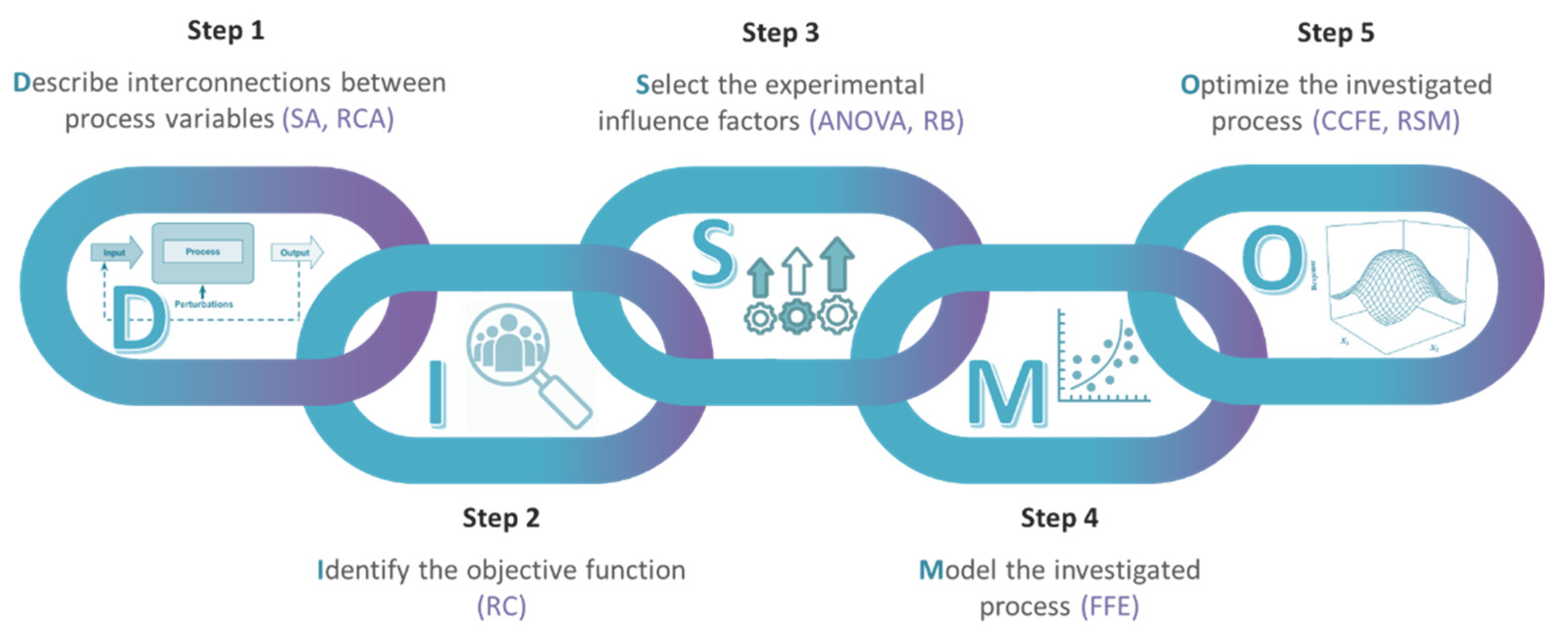
Figure 9.
Cybernetic model of the technological process.
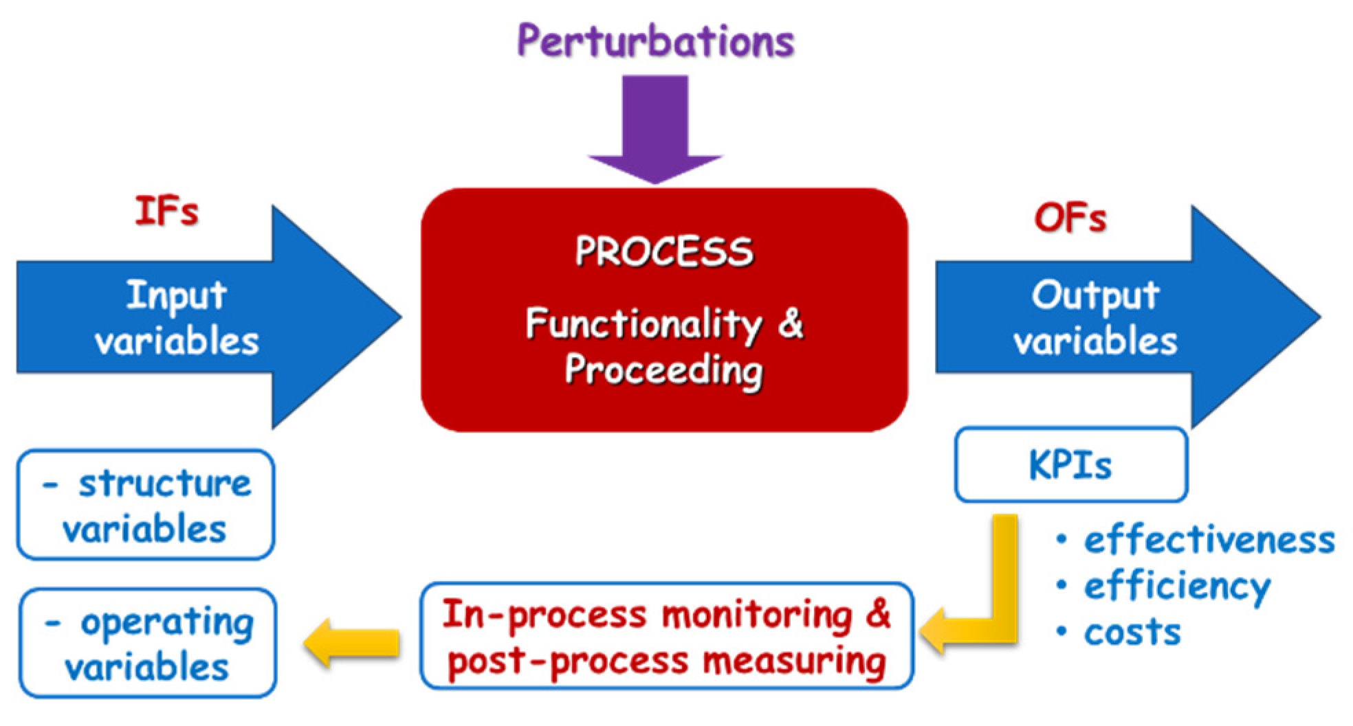
Figure 10.
Systemic analysis of direct dyeing process.
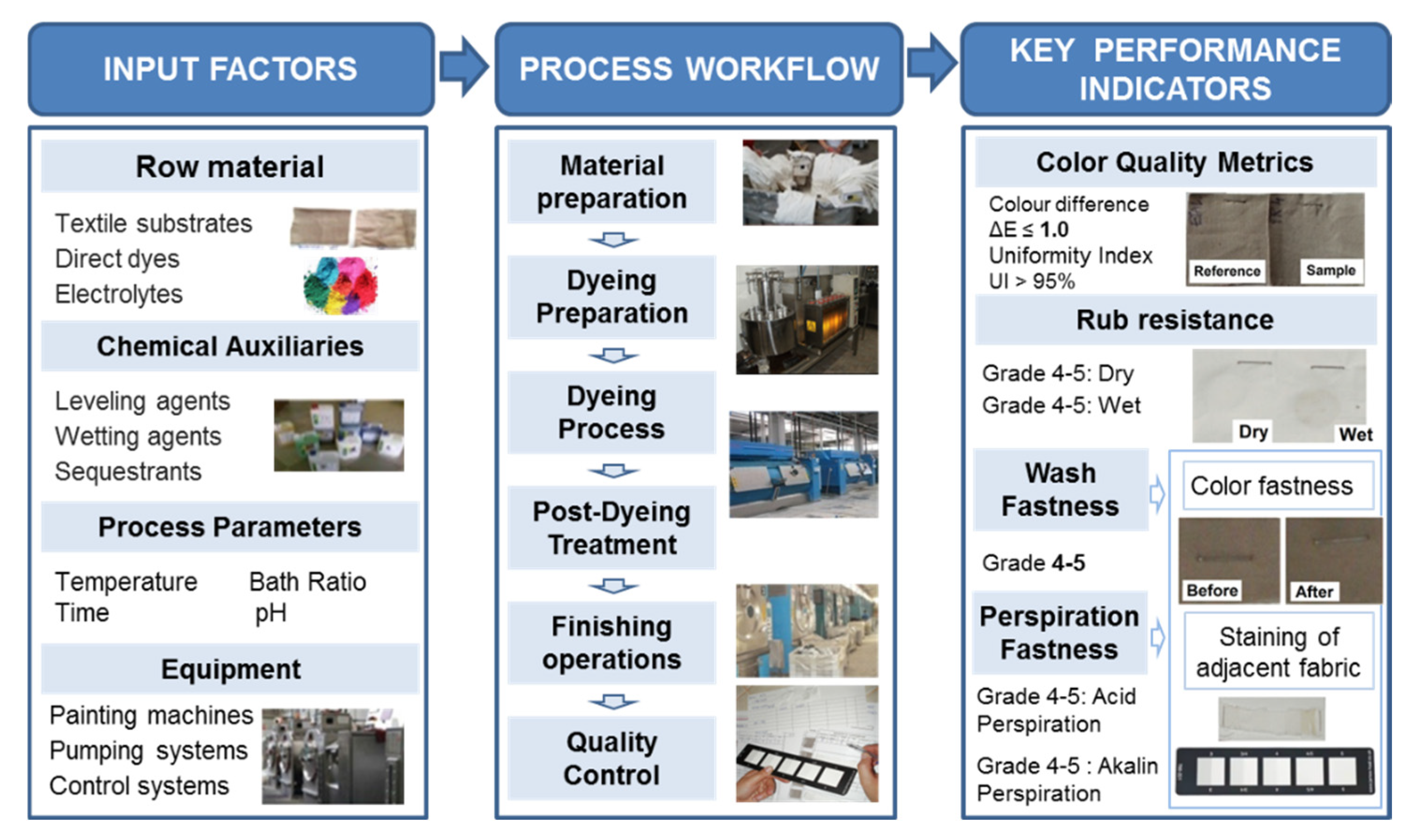
Figure 11.
Ranking of quality characteristics.
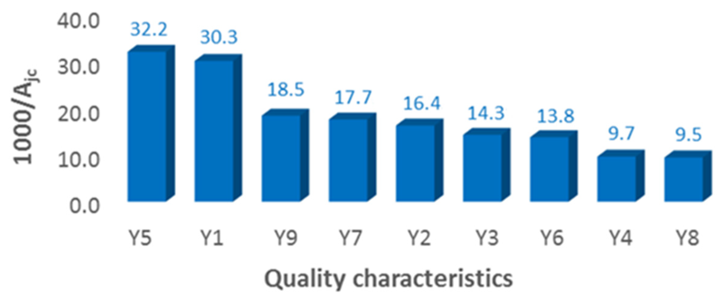
Figure 12.
Means plot of color difference ΔE: (a) for neutral electrolyte concentration; (b) for material (fabric) type.
Figure 12.
Means plot of color difference ΔE: (a) for neutral electrolyte concentration; (b) for material (fabric) type.
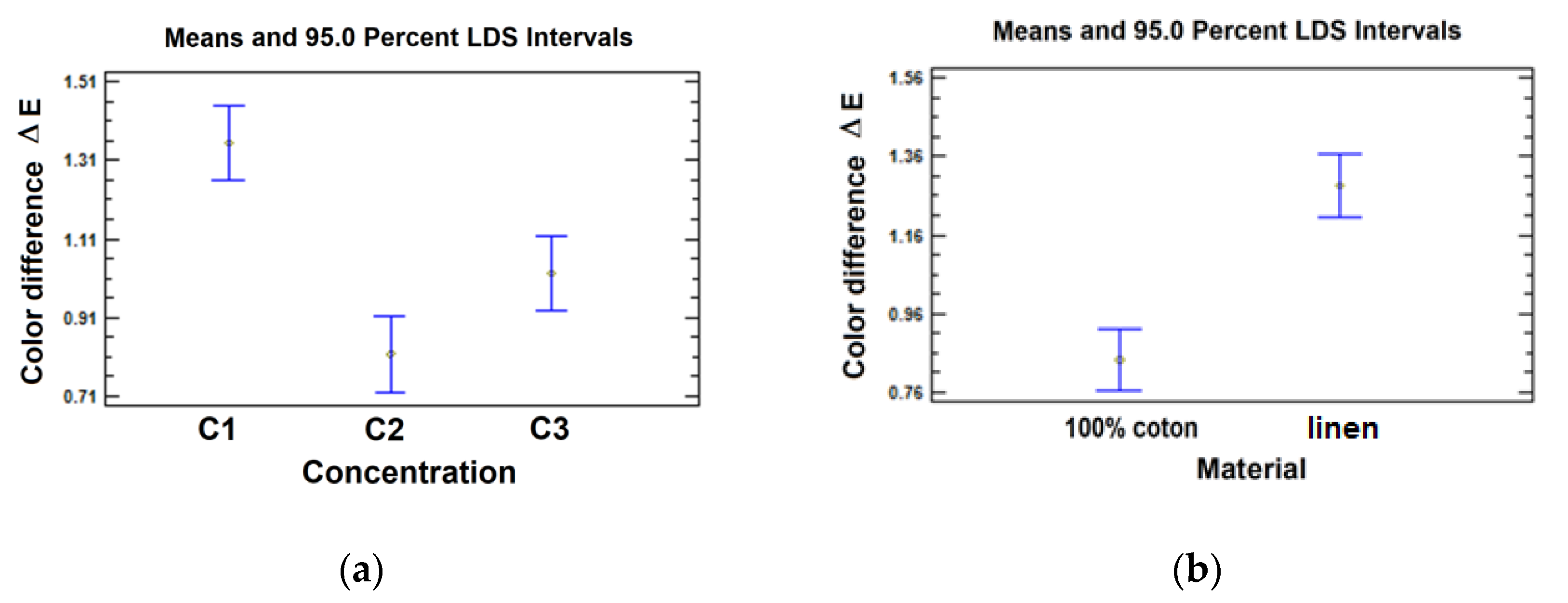
Figure 13.
Interaction plot for objective function ΔE.
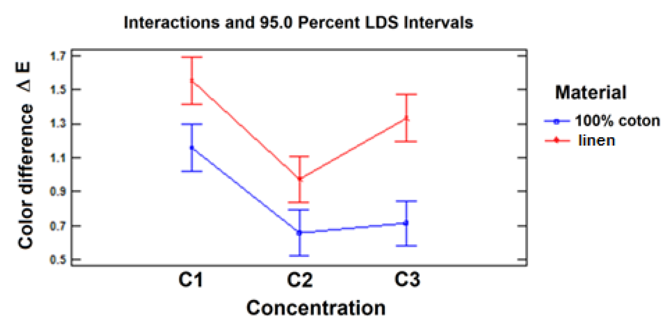
Figure 14.
Color difference ΔE measurement reports for 100% cotton and linen samples.
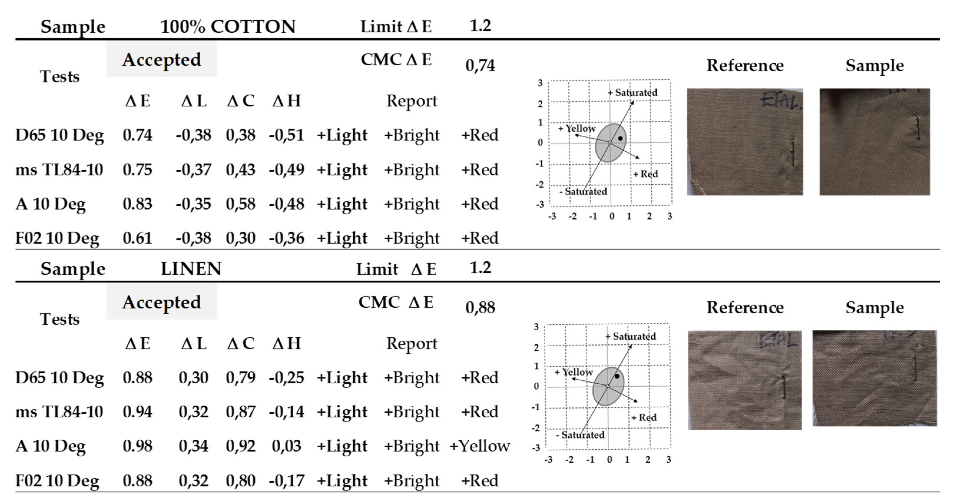
Figure 15.
Hierarchy of effects for objective function ΔE.
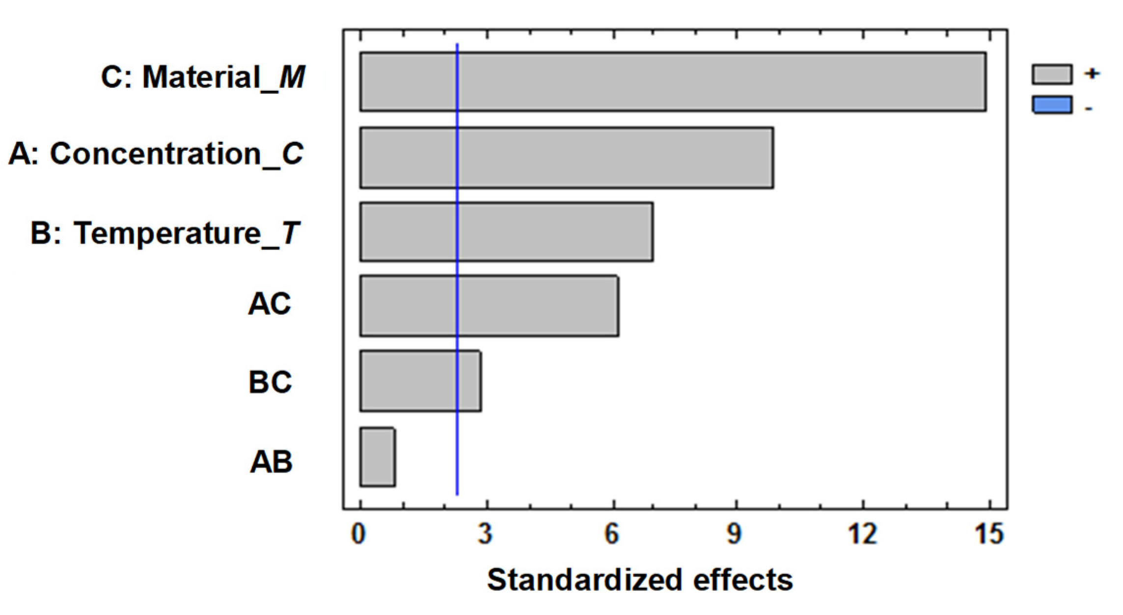
Figure 16.
Effects of factors on objective function ΔE.
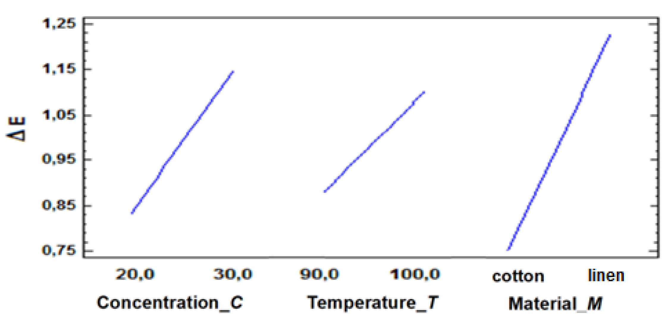
Figure 17.
Concordance diagnosis for objective function ΔE.
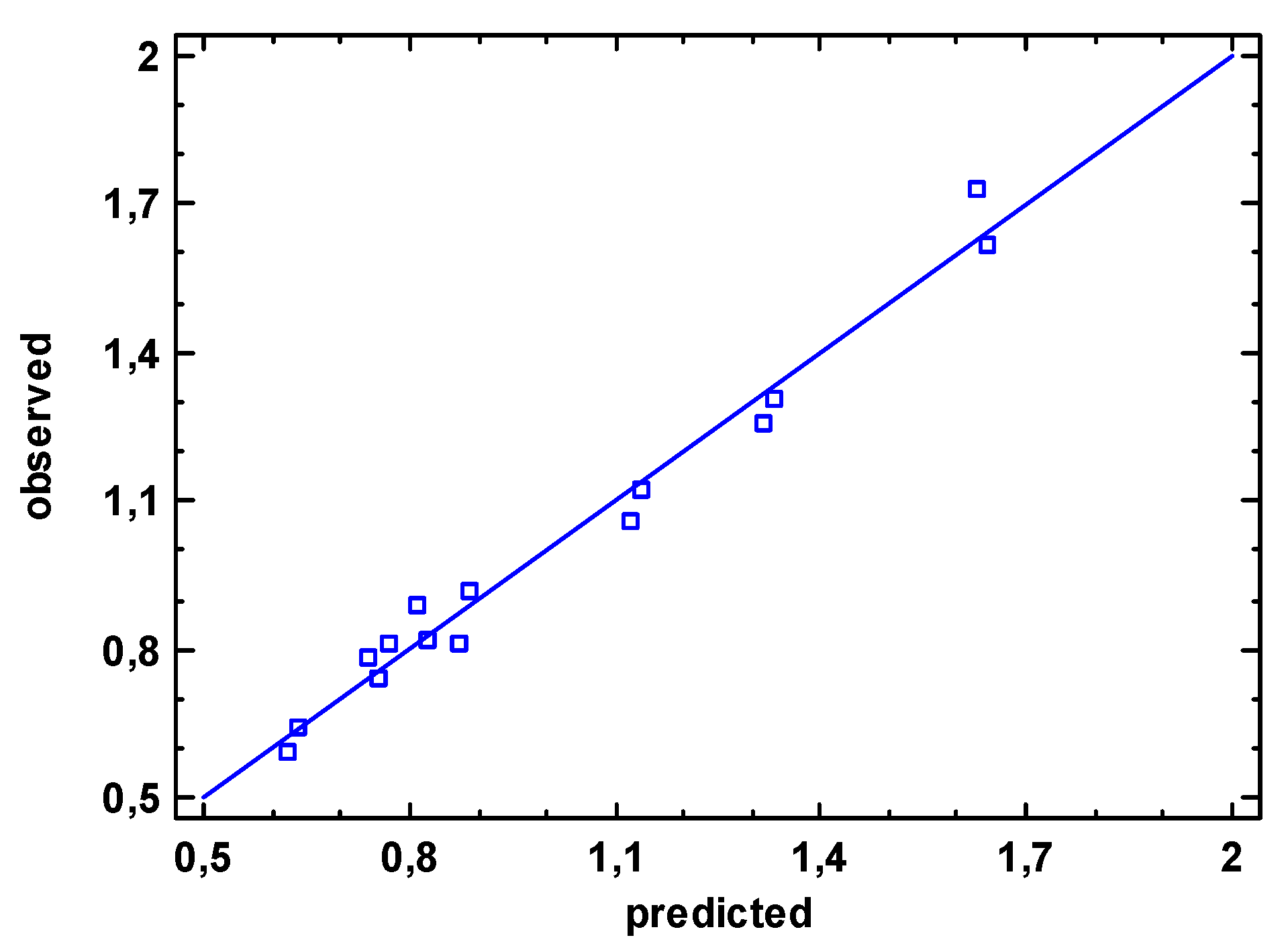
Figure 18.
Response surfaces of color difference ΔE versus neutral electrolyte concentration and bath temperature: (a) for 100% cotton; (b) for linen.
Figure 18.
Response surfaces of color difference ΔE versus neutral electrolyte concentration and bath temperature: (a) for 100% cotton; (b) for linen.
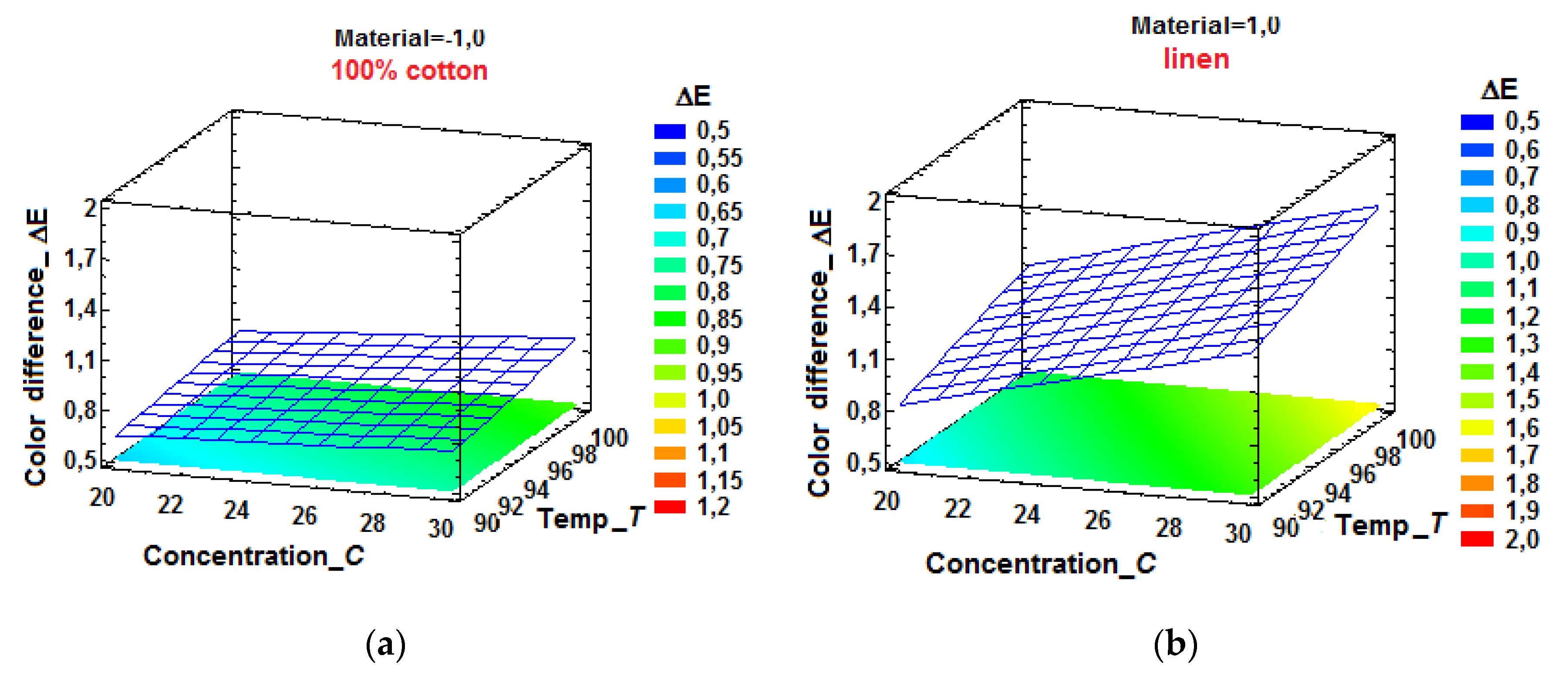
Figure 19.
Contour plots of color difference ΔE versus neutral electrolyte concentration and bath temperature: (a) for 100% cotton; (b) for linen.
Figure 19.
Contour plots of color difference ΔE versus neutral electrolyte concentration and bath temperature: (a) for 100% cotton; (b) for linen.
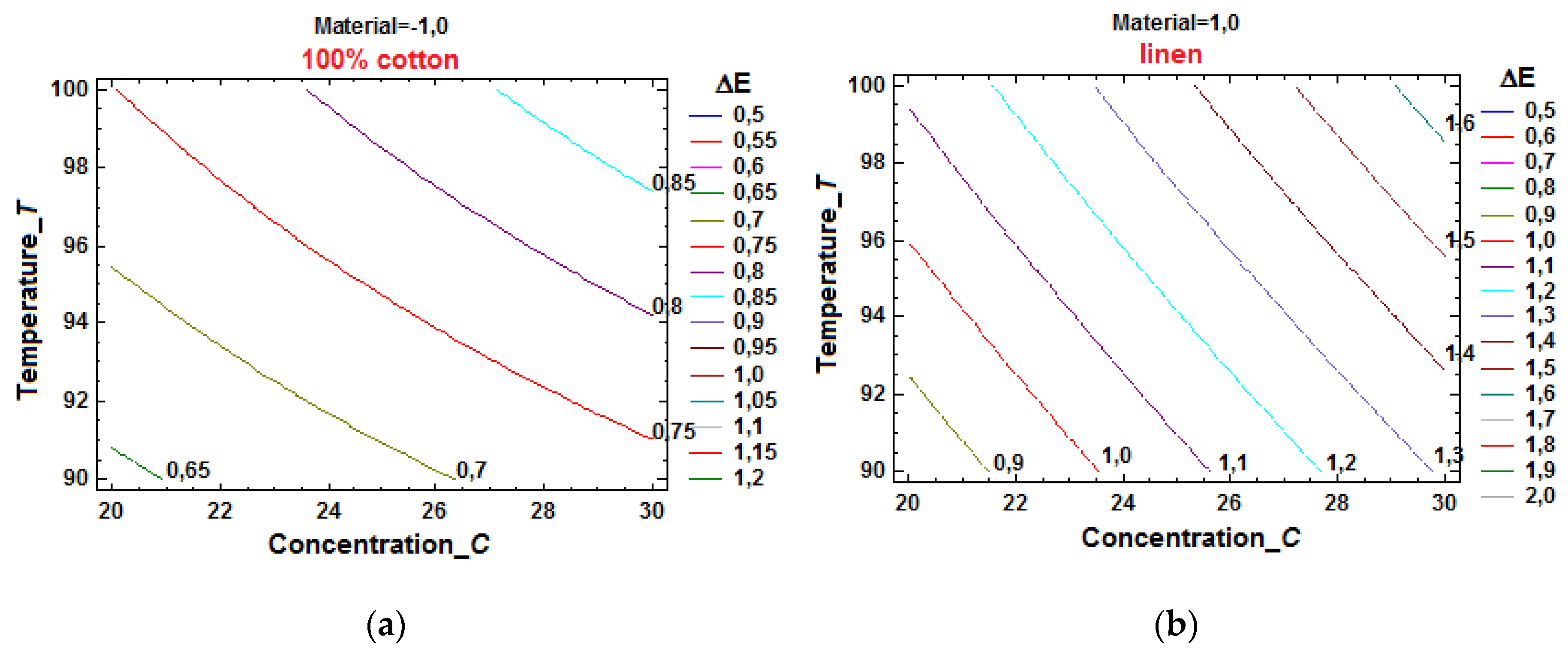
Figure 20.
The color fastness test results for the 100% cotton sample.
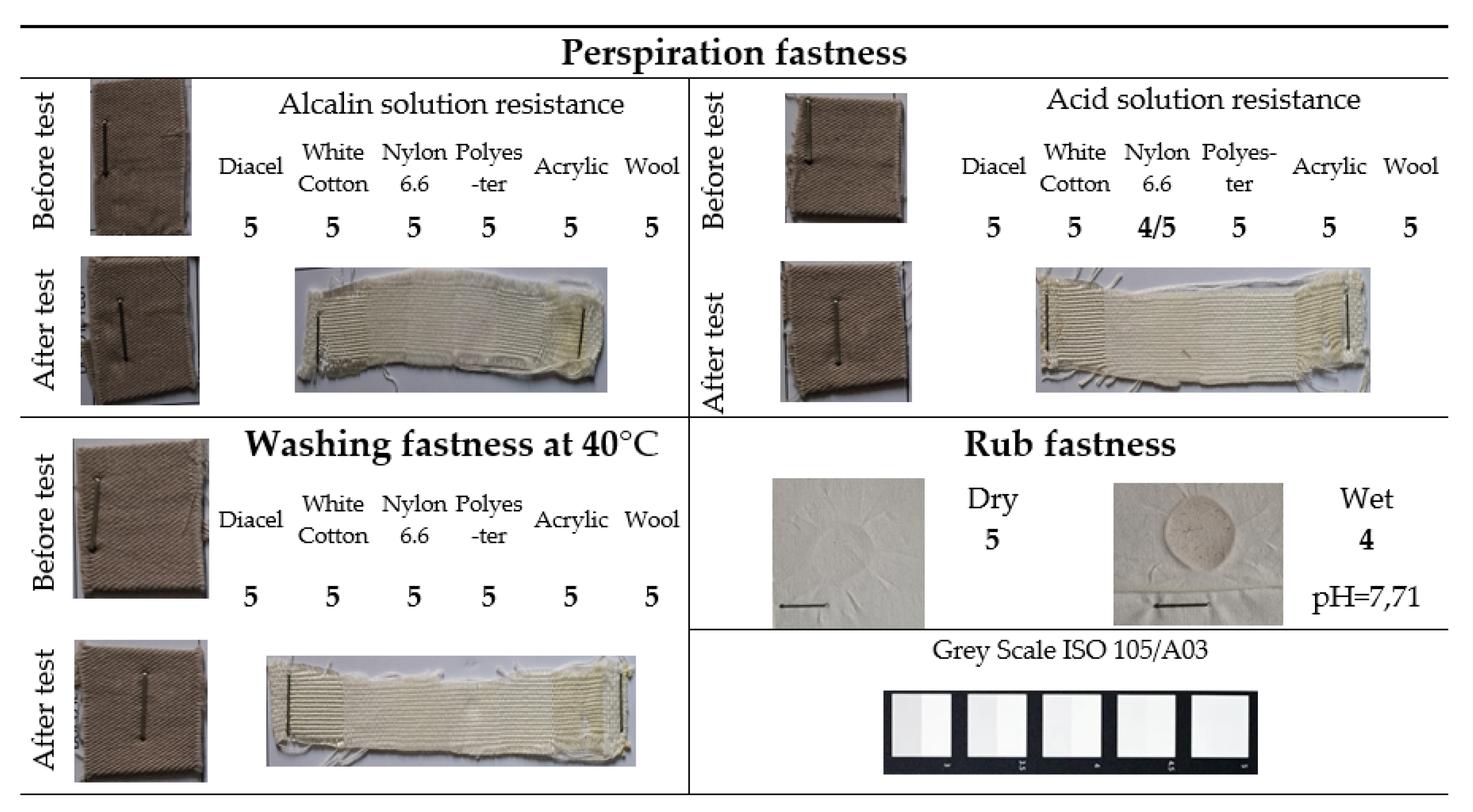

Table 1.
Direct dyes used during experimentation [27].
Table 1.
Direct dyes used during experimentation [27].
| Color Index No | Chemical Name | Commercial Name | Molecular Formula |
|---|---|---|---|
| 40291 | Direct Orange 39 | Direct Orange 2GL 120% | C46H28N8Na4O12S4 |
| 30145 | Direct Brown 95 | Direct Brown FRL/C | C31H20N6Na2O9S |
| 36250 | Direct Black 112 | Direct Gray GLL 200% | C58H34N15Na7O24S4 |
Table 2.
Initial order of quality requirements assigned by stakeholders.
| Stakeholder | Quality Characteristics | ||||||||
|---|---|---|---|---|---|---|---|---|---|
| CRi | Y1 | Y2 | Y3 | Y4 | Y5 | Y6 | Y7 | Y8 | Y9 |
| CR1 | 1 | 5 | 6 | 7 | 2 | 8 | 4 | 9 | 3 |
| CR2 | 1 | 3 | 4 | 5 | 2 | 3 | 6 | 4 | 5 |
| CR3 | 1 | 3 | 7 | 8 | 2 | 6 | 4 | 5 | 4 |
| CR4 | 5 | 4 | 7 | 9 | 3 | 1 | 2 | 8 | 6 |
| CR5 | 2 | 6 | 3 | 6 | 1 | 4 | 3 | 5 | 1 |
| CR6 | 1 | 2 | 3 | 9 | 5 | 6 | 7 | 8 | 4 |
| CR7 | 2 | 5 | 3 | 6 | 1 | 4 | 3 | 6 | 1 |
| CR8 | 3 | 8 | 6 | 7 | 1 | 5 | 4 | 9 | 2 |
| CR9 | 2 | 7 | 5 | 8 | 1 | 6 | 4 | 9 | 3 |
| CR10 | 6 | 3 | 2 | 4 | 1 | 1 | 1 | 5 | 4 |
| CR11 | 1 | 2 | 6 | 8 | 3 | 7 | 4 | 9 | 5 |
| CR12 | 2 | 1 | 4 | 7 | 5 | 6 | 3 | 8 | 6 |
| CR13 | 1 | 5 | 6 | 7 | 2 | 8 | 4 | 9 | 3 |
| Aj | 28 | 54 | 62 | 91 | 29 | 65 | 49 | 94 | 47 |
| Rj | 1 | 5 | 6 | 8 | 2 | 7 | 4 | 9 | 3 |
Table 3.
Corrected order of quality requirements assigned by stakeholders.
| Stakeholder | Quality Characteristics | Ti | ||||||||
|---|---|---|---|---|---|---|---|---|---|---|
| CRi | Y1 | Y2 | Y3 | Y4 | Y5 | Y6 | Y7 | Y8 | Y9 | |
| CR1 | 1 | 5 | 6 | 7 | 2 | 8 | 4 | 9 | 3 | 0 |
| CR2 | 1 | 3.5 | 5.5 | 7.5 | 2 | 3,5 | 9 | 5.5 | 7.5 | 18 |
| CR3 | 1 | 3 | 8 | 9 | 2 | 7 | 4.5 | 6 | 4.5 | 6 |
| CR4 | 5 | 4 | 7 | 9 | 3 | 1 | 2 | 8 | 6 | 0 |
| CR5 | 3 | 8.5 | 4.5 | 8.5 | 1.5 | 6 | 4.5 | 7 | 1.5 | 18 |
| CR6 | 1 | 2 | 3 | 9 | 5 | 6 | 7 | 8 | 4 | 0 |
| CR7 | 3 | 7 | 4.5 | 8.5 | 1.5 | 6 | 4.5 | 8.5 | 1.5 | 18 |
| CR8 | 3 | 8 | 6 | 7 | 1 | 5 | 4 | 9 | 2 | 0 |
| CR9 | 2 | 7 | 5 | 8 | 1 | 6 | 4 | 9 | 3 | 0 |
| CR10 | 9 | 5 | 4 | 6.5 | 2 | 2 | 2 | 8 | 6.5 | 30 |
| CR11 | 1 | 2 | 6 | 8 | 3 | 7 | 4 | 9 | 5 | 0 |
| CR12 | 2 | 1 | 4 | 8 | 5 | 6.5 | 3 | 9 | 6.5 | 6 |
| CR13 | 1 | 5 | 6 | 7 | 2 | 8 | 4 | 9 | 3 | 0 |
| Ajc | 33 | 61 | 69.5 | 103 | 31 | 72 | 56.5 | 105 | 54 | ∑Ti = 96 |
| Rjc | 2 | 5 | 6 | 8 | 1 | 7 | 4 | 9 | 3 | - |
| Δ j2 | 1024 | 19 | 20.25 | 1444 | 1156 | 49 | 72.25 | 1600 | 121 | ∑Δj2= 5502.5 |
Table 4.
Experimental results for Two-way ANOVA.
| Run No | Concentration | Material | ΔE (-) | Run No | Concentration | Material | ΔE (-) |
|---|---|---|---|---|---|---|---|
| 1 | C1 | cotton | 0.98 | 10 | C1 | linen | 1.45 |
| 2 | C1 | cotton | 1.31 | 11 | C1 | linen | 1.68 |
| 3 | C1 | cotton | 1.18 | 12 | C1 | linen | 1.53 |
| 4 | C2 | cotton | 0.74 | 13 | C2 | linen | 1.15 |
| 5 | C2 | cotton | 0.52 | 14 | C2 | linen | 0.88 |
| 6 | C2 | cotton | 0.71 | 15 | C2 | linen | 0.89 |
| 7 | C3 | cotton | 0.73 | 16 | C3 | linen | 1.16 |
| 8 | C3 | cotton | 0.52 | 17 | C3 | linen | 1.34 |
| 9 | C3 | cotton | 0.89 | 18 | C3 | linen | 1.49 |
Table 5.
Two-way ANOVA for the objective function ΔE.
| Source | Sum of squares | Degrees of freedom | Mean Square | Fisher Ratio |
p-value |
|---|---|---|---|---|---|
| A: Concentration | SSA = 0.890844 | dfA = 2 | MSA = 0.445422 | FA = 19.00 | 0.0002 |
| B: Material | SSB = 0.88445 | dfB = 1 | MSB = 0.88445 | FB = 37.73 | 0.0001 |
| AB | SSAB = 0.0724 | dfAB = 2 | MSAB = 0.0362 | FAB = 1.54 | 0.2531 |
| Residual | SSe = 0.281333 | dfe = 12 | MSe = 0.0234444 | ||
| Total (corr.) | SST = 2.12903 | dfT = 17 |
Table 6.
Multiple range test for the objective function ΔE – Method: 95.0 % LSD.
| Contrast | Significance | Mean difference | +/- Limits |
|---|---|---|---|
| C1 – C2 | yes | 0.54 | 0.192611 |
| C1 – C3 | yes | 0.333333 | 0.192611 |
| C2 – C3 | yes | -0.206667 | 0.192611 |
Table 7.
Experimental matrix of the FFE 23 and measured values of color difference, ΔE.
| Run No | A: C | B: T | C: M | Yi : ΔE (-) | ||||
|---|---|---|---|---|---|---|---|---|
| coded | (g/L) | coded | (°C) | coded | (-) | Yi1 | Yi2 | |
| 1. | -1 | 20 | -1 | 90 | -1 | cotton | 0.64 | 0.59 |
| 2. | +1 | 30 | -1 | 90 | -1 | cotton | 0.74 | 0.78 |
| 3. | -1 | 20 | +1 | 100 | -1 | cotton | 0.81 | 0.74 |
| 4. | +1 | 30 | +1 | 100 | -1 | cotton | 0.92 | 0.81 |
| 5. | -1 | 20 | -1 | 90 | +1 | linen | 0.82 | 0.89 |
| 6. | +1 | 30 | -1 | 90 | +1 | linen | 1.31 | 1.26 |
| 7 | -1 | 20 | +1 | 100 | +1 | linen | 1.12 | 1.06 |
| 8. | +1 | 30 | +1 | 100 | +1 | linen | 1.62 | 1.73 |
Table 8.
Calculated values of the regression coefficients for the objective function ΔE.
| Coeff. | Value | Coeff. | Value | Coeff. | Value | Coeff. | Value |
|---|---|---|---|---|---|---|---|
| b0 | 0.99 | b2 | 0.11125 | b12 | 0.0125 | b23 | 0.045 |
| b1 | 0.15625 | b3 | 0,23625 | b13 | 0.0975 | - | - |
Table 9.
ANOVA for the objective function ΔE.
| Source | Sum of squares | Degrees of freedom | Mean Square | Fisher Ratio | p-value |
|---|---|---|---|---|---|
| A: C | 0.390625 | 1 | 0.390625 | 96.97 | 0.0000 |
| B: T | 0.198025 | 1 | 0.198025 | 49.16 | 0.0001 |
| C: M | 0.893025 | 1 | 0.893025 | 221.70 | 0.0000 |
| AB | 0.0025 | 1 | 0.0025 | 0.62 | 0.4535 |
| AC | 0.1521 | 1 | 0.1521 | 37.76 | 0.0003 |
| BC | 0.0324 | 1 | 0.0324 | 8.04 | 0.0219 |
| blocks | 0.0009 | 1 | 0.0009 | 0.22 | 0.6491 |
| Total error | 0.032225 | 8 | 0.00402812 | ||
| Total (corr.) | 1.7018 | 15 |
Disclaimer/Publisher’s Note: The statements, opinions and data contained in all publications are solely those of the individual author(s) and contributor(s) and not of MDPI and/or the editor(s). MDPI and/or the editor(s) disclaim responsibility for any injury to people or property resulting from any ideas, methods, instructions or products referred to in the content. |
© 2025 by the authors. Licensee MDPI, Basel, Switzerland. This article is an open access article distributed under the terms and conditions of the Creative Commons Attribution (CC BY) license (http://creativecommons.org/licenses/by/4.0/).
Copyright: This open access article is published under a Creative Commons CC BY 4.0 license, which permit the free download, distribution, and reuse, provided that the author and preprint are cited in any reuse.


