
Submitted:
28 September 2025
Posted:
30 September 2025
You are already at the latest version
Abstract
Many systems exhibit multistage mechanisms where failure of any single component leads to overall failure. Standard logistic regression, with its additive log-odds structure, is not well suited for such data-generating processes. We propose the Multistage Binomial (MSB) model, an extension of the binomial generalized linear model in which component effects combine multiplicatively on the success-probability scale. The MSB model naturally accounts for unobserved components by allowing the success probability to asymptote below one. It additionally incorporates measurement variability in explanatory variables through a Berkson-type error framework. We establish conditions for identifiability, develop a penalized maximum likelihood estimation procedure, and a non-standard likelihood ratio test for unit asymptote. Using synthetic data on mutated protein viability, we show that the likelihood ratio test is conservative, and only rejects the unit asymptote assumption when it is strongly supported by data. We also demonstrate that the MSB model provides more accurate inference and prediction than traditional logistic regression in multistage settings. Our simulations further show that larger sample sizes are required with increased proportion of unobserved components. We provide a chart for sample size determination under an MSB design for real data analysis given the desired accuracy and the distribution of predictors.
Keywords:
multistage process
; binomial regression
; Berkson measurement error
; Jeffreys invariant prior
; mutation viability
1. Introduction
Binomial data are routine in quantitative sciences, naturally arising for instance in biology (e.g. presence or absence of a particular disease, a mutation leading to a viable or an unviable protein, survive or not survive the great migration in the Serengeti), economics (e.g. purchase or not purchase a product), material science (chiral or achiral compound, presence or absence of defects), and behavioral science (e.g. voting, school dropout, divorce). Binomial regression is the modern approach to analyzing such dichotomous outcomes, and most researchers turn to the logistic model [1,2,3].
In the Generalized Linear Model (GLM) framework [4], the logistic regression model for a binary outcome Y assumes a log-linear odds ratio for the success event versus the failure , i.e. the expectation (also the success probability) of Y satisfies
where () are explanatory variables for Y, and () are regression coefficients. Stated, otherwise, the effects of the predictors of the odds ratio of the event are multiplicative. The logistic assumption (1) is mathematically convenient, allowing an unrestricted parameterization of the binomial GLM: the coefficients (which measure changes in the log-odds ratio) take values on the entire real line.
Despite the popularity of the standard logistic regression (multiplicative odds) for binary outcomes, the underlying assumption of this model does not cover phenomena resulting from many independent or successive discrete events. Indeed, complex systems often progress through a series of rate-limiting steps which can be subject to modifications by environmental exposures [5]. There can thus be a large number of routes to the failure of such systems, but only the final state is often observable. Indeed, many physical processes can be described by a number of specific events occurring randomly or in some predetermined order. In other words, the occurrence of a particular event often depends on the prior occurrence of many other (partially) related events.
Examples of such events are common along a manufacturing chain: the absence of defects on an end-line product obtained from assembling q different pieces depends on the occurrence of defects in each assembly line producing a piece. If the lines are independent, then the probability of a defect-free final item is the product of the no-defect probabilities in the q lines ():
Of course, the design of products is generally optimized so as to make errors additive and the effect of a single defect as insignificant as possible. However, if only the presence or absence of defects is of interest, then the multiplicative absolute risk model (2) reflects the process generating the binary outcome.
Processes with multiplicative risks are in fact common in biology, since many biological processes involve discrete events, at least at some levels of description and observation [6,7]. Consider, for instance, a mutated protein resulting from a single amino acid substitution, with functional viability depending upon two factors: the protein’s ability to fold into a native conformation (related to folding stability), and its ability to bind other subunits or ligands (related to binding stability). If such a protein does not fold properly (e.g. because of a highly destabilizing mutation), it is likely not going to bind (very low probability) since most proteins only bind their targets when folded [8]. The viability of the mutated protein is thus proportional to the probabilities of folding () and binding (): so that any predictor value leading to a small probability begets an overall prediction near zero (i.e. a mutation that renders a protein able to fold, but not bind, or vice versa, should be inviable). In this specific case, the multiplicative odds model (1) appears particularly inappropriate. Indeed, for with and representing folding and binding stabilities, respectively, if we fix folding stability to a value , then it is always possible to find some value of binding stability so that the viability gets arbitrarily close to one (including an interaction term into (1) does not help because this is simply equivalent to adding to ). This contradicts the fact that when folding stability is disrupted, the functional viability of the mutated protein cannot get arbitrarily close to one, regardless of the binding stability.
More generally, a multiplicative risk model arises naturally for any all-or-none type event. For instance, the presence or absence of a disease may result from the total absence of one or more protective events (e.g. diet deficiencies in required dietary constituents leading to a resultant disease) [9,10]. Conversely the presence or absence of a particular disease may result from one or more adverse events (e.g. encounters with carcinogenic agents leading to a specific cancer). Multiplicative risks are indeed widely used, for instance, in multi-stage cancer models [11,12,13,14,15,16,17], and for incidence or hazard rate models in survival analysis [18,19,20]. In social epidemiology, many studies reported evidence for multiplicative relations between the effects of risk factors and disease incidence or mortality [21,22,23,24,25].
However, to the best of our knowledge, there is no general binary data model with multiplicative absolute risks. To overcome interpretation difficulties related to the non-collapsibility of odds ratio [26,27,28,29,30], some works considered log-binomial models where, as in a Poisson GLM, covariates have multiplicative effects on the relative risk [31,32,33,34]. In addition, the Zero-Inflated Bernoulli (ZIB) model, a special case of the zero-inflated binomial model [35], is related to the multiplicative risk model (2); as we discuss in Section 2, the ZIB model can be described as a special case of our proposal. In spite of some recent developments in relative risk modeling where the probability of the target event is modeled as a ratio to the probability under a reference condition [36,37], these models not only lack the mathematical convenience of the logistic model (sample dependent constraints required on the parameter space to ensure that predicted probabilities are restricted to , or restricted ranges of covariates), but also have their own set of interpretation issues [38,39,40,41].
We propose in this work an extension of the Traditional Binomial (TB) model to handle binomial data resulting from data generation processes with known multiplicative risk components. The proposed model assumes that in addition to an observed binomial outcome, we are aware of some unmeasurable prior events that determine the final outcome (with paths to success or failure involving sequential, or non-sequential steps, or a combination of both), and each prior event is known to be related to a subset of the observable explanatory variables. The proposal results from combining equation (2) with a standard binomial model inverse link function, i.e. each factor is given by with and a linear predictor obtained from explanatory variables related to . Most popular binomial model link functions include the logit link function (1) with inverse the cumulative distribution function (cdf) of the logistic distribution,
and the probit link with where is the cdf of the standard normal distribution. The resulting model is termed Multistage Binomial (MSB) model. It is worthwhile emphasizing that the MSB model (with multiple stages) is not a generic model for binomial data. Its use should be prescribed by some theoretical or empirical knowledge of the phenomenon being modeled. In case of only a (theoretical) suspicion of multiple stages, the MSB model should be tested against the TB model.
In addition to providing a general framework for modeling multiplicative risks in binomial data, nesting the TB and ZIB models, our proposed MSB model allows to control for two important sources of issues in statistical analysis: omitted variables and measurement errors in predictors. Indeed, researchers can seldom be aware of, let alone measure, all of the variables that determine a target outcome, and the impact of left out or omitted variables can be dramatic for interpretations in TB models [42,43,44,45,46,47,48,49,50]. Our formulation of the MSB model allows to control for omitted variables in some variable omission scenarios, i.e., when the explanatory variables which determine some factors in (2) are omitted. Moreover, observed predictors are often error-prone. To account for errors in observed explanatory variables, the proposed MSB model also allows for heteroscedastic additive Berkson measurement errors [51] when the variability of each numerical predictor around its observed values is known.
For inference in the MSB model, we developed a Penalized Maximum Likelihood (PML) estimation procedure. The PML method has two main advantages over a simple Maximum Likelihood (ML) approach: reduce small sample bias and circumvent estimation issues related to quasi or complete separation. On the one hand, although ML estimates in TB regression are asymptotically unbiased to first order, it is well known that the ML estimators are biased to first order in small sample ( [52,53]). This occurs especially when the marginal success probability of the response approaches zero or one [54]. The ML estimators of the MSB model parameters are also expected to be biased to the first order in small samples because this is a general feature of binomial regression models [55].
On the other hand, complete separation occurs when one or more of the explanatory variables can perfectly predict some binary outcomes [56]. Quasi separation occurs when for any values of an explanatory variable (or a linear predictor) less than a threshold, say , the binary outcome is always (or always ), but when , might equal zero or one. The occurrence of (quasi) separation is generally related to small sample, sparse data, rare outcome ( is very small), rare exposures (and more generally predictors with very small variability), large number of dichotomous risk factors [57], and highly correlated predictors (multicollinearity) [58], or covariates with strong effects [59].
Since the MSB model can be viewed as a combination of many TB regressions across stages of a complex process, the occurrence of separation becomes more likely not only as the number p of predictors in any stage increases, but also as the number q of stages increases, for not sufficiently large samples. As a consequence, in the MSB model framework, we anticipate an increased likelihood of unrealistically large ML estimates or related large (or undefined) standard errors as p or q increases, and as the sample size n or the maximum success probabilities decrease. Quasi or complete separation implies that maximum likelihood estimates approach infinity or zero [60,61]. In practice, separation generally results in a flat log-likelihood surface (likely with an asymptote) which leads to implausible estimates, and no or very large standard error estimates [62].
In this paper, we investigate some theoretical and numerical properties of MSB models. We first study the identifiability of the proposed model. Then, using simulation experiments, we study finite-sample properties of the PML estimates of the MSB model parameters. Specifically, we i) compare, for demonstration purposes, the Two-Stage Binomial (TSB) model to TB and ZIB models considering a simulated biological case study on the viability of a mutated protein; ii) assess the ability of PML estimators of MSB to recover the population values of regression parameters and predict event success probabilities in finite samples; iii) and evaluate finite-sample properties of a non-standard Likelihood Ratio (LR) test to motivate the choice of the MSB model over alternatives such as the TB or ZIB model.
2. The Multistage Binomial Model
The MSB model is built as an extension of the standard binomial GLM [4]. In this section, we specify and describe the main features of the MSB model, starting with the simpler model in the absence of measurement errors in observed covariates, and then introducing measurement errors. We then establish and discuss conditions for the identifiability of the model. Finally, we describe the estimation of model parameters using Jeffreys invariant prior as likelihood penalty, and an LR test to the detect omission of important process stages or predictors.
2.1. Measurement Error-Free Model
Let us consider a design with n units indexed i, each having (known positive integer) independent Bernoulli trials. The binomial outcome is assumed to be generated through a multistage process with q known steps, each related to a -vector of covariates (). The multiplicative risk binomial model is given for the ith outcome as:
where is the vector of covariates; denotes the binomial distribution with trials and success probability ; is the upper limit of the success probability () of each Bernoulli trial given and is such that is the lower limit of ; h is the inverse link function for the binomial outcome (h is assumed to be a continuous cdf, monotone, increasing and twice differentiable); and is a -vector of real regression parameters (possibly including an intercept ).
Model (4) describes a binomial process where the outcome results from q latent stages where each stage is represented by an independent Bernoulli experiment, and the final outcome corresponds to all experiments being simultaneously successful. As indicated above, the success probability is bounded as . These bounds represent theoretical limits that may arise from some unknown stages, or some known stages with no measured explanatory variable. Indeed, setting without loss of generality, and starting from multiplicative risks of the form (2) with stages () among which the first () is omitted, the conditional success probability of the outcome given the measured covariates is then
where is the success probability at the omitted stage, averaged over of the distribution of the related -vector of explanatory variables, which has joint density function (integration will be replaced by summation where is a probability mass function (pmf), i.e., if is discrete).
Stated in other words, the omission of explanatory variables related to a stage in the multiplicative-risk model (2) leads to (4b) with . It is worth noticing that while this rationale applies to unobserved confounders that vary across experimental or observational units, it remains valid when the vector of predictors of a stage is (willfully or not) held constant across all investigated/sampled units: in this case, is not an average of success probabilities across the possible values of , but rather the conditional success probability of this stage given the constant value of : .
This development indicates that can arise from one or both of two potential sources: uncontrolled confounders (marginalization), or a limit of the data generation mechanism in the specific investigated experimental or observational environment/condition (conditioning). In the general formulation (4) of the MSB model, we allow to vary across observations to potentially account for conditioning when the study is replicated across some discrete experimental/environmental settings: can capture the maximum success probability for all units i from the same setting. For the sake of symmetry, is allowed in model (4): since, one can equivalently model the failure of an event to occur instead of its success, the minimum success probability can also be greater than zero. By the same reasoning, this rationale can be extended to the omission and marginalization over many stages, or conditioning on one value of the vector of predictors at each of many stages.
Remark 1.
When model (4) has only one () or two stages (), we obtain the following two important special cases.
- When , , and , the MSB model is reduced to the TB model.
-
For binary outcomes ( for ), when , , and , the MSB model is reduced to the ZIB model.The ZIB model has been proposed by Hall [35] to face situations where a binary outcome contains an excess of zeros as compared to the expected zeros under the TB model. The ZIB model assumes that the binary outcome is the product of two Bernoulli processes; a zero from either process (or both) results in a zero. An example of process generating such data in health sciences was investigated by Diop et al. [63]: a study population consisting of a mixture of susceptible subjects who can experience the binary outcome of interest, and cured subjects (cure fraction) who cannot experience the binary outcome. Complications arise from not knowing the immunity (cured or susceptible) status of each subject, and the ZIB model is used to jointly estimate the cure fraction on the one hand, and the logistic regression for the susceptible subjects on the other hand [64,65,66]. Using the MSB model framework (, , , and ) to describe the ZIB model, the success probability of the binary outcome is and the probability that a subject i is cured is . Thus, in this case, the main difference between the MSB model and the ZIB model is that the MSB model allows the minimum probability to be greater than zero, and the maximum success probability to be less than one.When the susceptibility probability is constant across subjects in the ZIB model, the latter can alternatively be considered as a one stage model () with and . In this case, the success probability of the binary outcome is and the probability that a subject i is cured is .
In complement to Remark 1, it is worthwhile emphasizing that the MSB model is not a zero inflation model, nor a mixture model for count data. These models only share some special cases with the MSB model when each and every count is binary. For general binomial data, the zero-inflated binomial model [67] is not a special case of the MSB model, even when .
Remark 2.
An ovulation-time model was developed by Garel et al. [68] to investigate how the probability of ovulation and body growth co-evolve over time in moose. The special case of the probit link MSB model when , and , is closely related to the ovulation-time model. In the MSB model framework, the first stage in their model represents susceptibility to ovulation at a time, and the second stage is the occurrence of ovulation (this also points to a close relation with the ZIB model). However, unlike the fixed-scale link used in proper binomial models, the ovulation-time model employs a covariate-dependent probit link scale to capture spatiotemporal dynamics in the occurrence of ovulation.
2.2. Multistage Binomial Model Specification
In practice, the covariates in model (4) can be observed with measurement errors. We consider a situation where is error-prone: instead of , we only have access to an observable such that satisfies:
where is a measurement error vector independently following an unspecified zero-mean distribution,
which has covariance matrix (a known semi-positive definite matrix), and a probability density function (pdf) . The measurement error in (6) is known as an additive Berkson error [51]. This error model is appropriate when a subset of the available explanatory variables are obtained from an estimation process such that the observed can be regarded as an estimate of the truth , and is an estimate of the covariance matrix of .
For inference purposes here, we are interested in the expected value of the outcome given an observed covariate vector : where is the number of trials, and is the success probability given . The Multistage Binomial (MSB) model is defined as:
where and are as defined in (4), and is obtained for by integrating out the measurement error vector as:
with (summation replaces integration where is a pmf, i.e., if is discrete). From the conditional expectation , the conditional variance of the binomial outcome is
When there is no measurement error (), we have and from , hence . It follows that the measurement error-free model (4) is a special case of the MSB model (8) when for all stages ; and across all units .
A design for the general MSB model (8) includes the response vector of n independent outcomes, the associated (with ) design matrix , and the array of known covariance matrices of measurement errors. Because the MSB model allows the success probability bounds and to vary across experimental or observational units, the complete design includes two additional design matrices and where is a d-vector and is an r-vector such that and , and and are parameters that determine the success probability bounds. In particular, each of and may have a fixed value across units, i.e., we can have (n-vector of all ones) and so that and with , , (). In practice, we may also allow empty and (), i.e., and have fixed and known values, e.g. and for all .
As motivated in Section 2.1, the additional covariates making and/or vary across units should be discrete, i.e. each and should be binary/contrast matrices (obtained by an appropriate coding of some categorical predictors) for the MSB model (8). As such, categorical predictors describing site conditions should be included into the design matrices and to define multiplicative intercepts for groups. Any stage of the considered multistage process can also include categorical variables. In the presence of categorical predictors, the MSB model becomes a multistage analogue of the analysis of covariance model for a binary response: categorical predictors define groups with different intercepts in the study population [69].
2.3. Conjugate Distribution for Measurement Errors
The possibly multivariable integrals (9) in the MSB model specification can make model estimation a difficult task requiring integral approximation methods such as Gaussian quadrature [70,71], or EM-type algorithm [72,73] which can be computationally demanding. To circumvent such difficulties, we consider an implicit conjugate distribution for measurement errors, such that each integral (9) is tractable. As per Proposition 1 below (see a proof in Appendix A.1), under this conjugate distribution of measurement errors, the integral (9) is given by the inverse link function h.
Proposition 1
(Conjugate measurement error distribution). Assume that the probability distribution corresponding to the link function h in the MSB model (8) has a finite variance . Then, there exists a family of distributions such that the function defined in (9) satisfies
where and .
Remark 3.
The conjugate ME distribution is known for popular link functions.
- For the logit link, and the conjugate distribution of measurement errors is the distribution such that the linear combination follows a logistic Bridge distribution (which is the conjugate distribution of random-effects in marginalized mixed effects logistic models [74]).
- For the probit link, and the conjugate measurement error distribution is the normal distribution with null mean vector and covariance matrix . This follows by Proposition 4 in [75].
From here on and afterwards, we restrict attention to the measurement error distribution implied by (11), unless otherwise specified. Under the conjugate assumption, the success probability in (8b) satisfies:
where , , , and .
2.4. Regularity Conditions and Identifiability
The MSB model (8) is parameterized by the m-vector of all unknown parameters with , . If or have known values (e.g. and ), the corresponding sub-vectors ( and ) are empty ( and , and ). Classical inference on is achieved by the ML approach. For inference purposes, we present here the log-likelihood function of the MSB model. Recall that the pmf of a binomial distribution with trials and success probability has the form [76]
By the pmf (13), the log-likelihood of a parameter vector given a sample of n independent units reads
where is as defined in Equation (12).
Let us denote as the vector of true model parameter. We require the following regularity conditions to ensure the identifiability of the MSB model, i.e., the ability to infer the parameter vector from observed data.
- C1-
- All predictors in the MSB model are bounded, i.e., there exist compact sets (for ), and such that , , and for every . For every , for , for , and for . For every , , and , the are linearly independent. For every and , and the are linearly independent, and for every and , the are linearly independent.
- C2-
- The true parameter vectors , and lie in the interior of known compact sets for , , and respectively.
- C3-
- There exists, for each stage j, a continuous predictor which is in but not in any (for all ), nor in , neither in . Moreover, there exists at least one continuous predictor, either in but not in nor in (for all ), or in but not in nor in (for all ).
The conditions C1–C3 are extensions of the corresponding conditions in Diop et al. [63]. The assumptions C1 and C2 are classical requirements for identifiability in the TB model. With regard to condition C3, it ensures that the product in (8b) is not invariant under any permutation of the parameter vectors (), and .
Remark 4.
- -
- In fact, the motivation of the MSB model assumes that we have some prior knowledge of the steps of the multistage process that generates the binary outcome . This implies that, for each step that we are aware of, we know about at least one specificity that differentiates it from other known steps. This is reflected by condition C3. If our prior knowledge of the steps of the process is confused to the point that two stages share the exact same predictors or risk factors, then we should consider that the two stages are only one known (meaningful) stage.
- -
- If all stages of the modeled process are known and accounted for, the model approaches the limiting special case where and . In this situation, the distinct continuous predictor in each of the q stages (condition C3 is only required for stages. That is, one of the q stages may not have a distinct continuous predictor.
- -
- A continuous predictor is required in the design matrix of either ( in ) or λ ( in ) only if both and are being estimated. For instance, in the important special cases where either or , no distinct continuous predictor is required in any of and design matrices, if present.
Based on the conditions C1–C3, Proposition 2 establishes identifiability of the MSB model (8) (see a proof in Appendix A.2).
Proposition 2
(Identifiability of an MSB model). Under the conditions C1–C3, the MSB model (8) with a logit or probit link function and the conjugate measurement error distribution is identifiable; i.e., almost surely implies .
Remark 5.
Proposition 2 considers the case of conjugate measurement error distribution with known error covariance matrices . Note that this includes the special case of no measurement error (). Some extensions are also readily available.
- For a logit link function, Proposition 2 remains true if the conjugate measurement error distribution were replaced by the (multivariate) normal distribution with null mean vector. This follows from Theorem 1 of Shklyar [77], given that the error covariance matrices are assumed known in the MSB model (8).
- In the case , the model remains identifiable if all covariance matrices are only known up to a unique scaling factor (see Theorem 2 of Kuchenhoff [78]). In particular, if the unique stage includes only one error-prone continuous predictor, then under conditions C1–C3, a homogeneous variance of the measurement errors is identifiable along with all other model parameters. Extension to requires further investigations.
It is important to observe that a null true model parameter is not generally identifiable (unless , and and are known constants, which essentially corresponds to the standard binomial model). Indeed, the condition C3 implies that some continuous predictors in the design matrices must have non-zero regression slopes. That is, the vector of true regression coefficients in each stage j must have at least one non-zero slope.
Also note that along with C1 and C2, condition C3 is sufficient for identifiability of the MSB model (8), but may not be required. That is, identifiability may also be established under some alternative conditions replacing C3. These may be physical or biological constraints on the predictors in each stage of the model, or restrictions on model parameters. For instance, in their probit link ovulation-time model, Garel et al. [68] imposed constraints on the parameter space (some coefficients were set to zero) to ensure numerical identifiability.
2.5. Penalized Maximum Likelihood Estimation
The ML estimates of the MSB model (8) parameters can be obtained by solving the score equation . The score function of the MSB model is given in Appendix B. To reduce bias in MSB parameter estimates for small samples and address quasi or complete separation issues, we consider a likelihood penalization approach which is the common route to first order bias correction in the standard logistic regression model [55,60,79,80,81]. For general exponential family models under canonical parametrization, Firth showed that using Jeffreys invariant prior as likelihood penalty removes the first-order bias term in the asymptotic expansion of the ML estimator [55]. The Jeffreys penalty, which is the square root of the determinant of the Fisher information matrix [82], is asymptotically negligible. As a result, the maximum a posteriori estimator is equivalent to the ML estimator in large samples.
For Penalized Maximum Likelihood (PML) estimation of MSB parameters based on the Jeffreys invariant prior, the penalized log-likelihood function is given by
where returns the logarithm of the determinant of its matrix argument and denotes the Fisher (expected) information matrix: [83]. The PML estimators of the MSB model parameters are obtained by solving the penalized score equation . The Fisher information of the MSB model as well as the penalized score are given in Appendix B. For inference in the MSB model, we implemented both the ML and PML procedures in the open source library msbreg (available at https://github.com/Chenangnon/msbreg) in R freeware [84].
2.6. Testing for Unit Asymptote
One important feature of the proposed MSB model framework is the ability to infer the absence or not of unknown stages that significantly affect the binomial outcome. Indeed, when there is no controlled experimental condition making the maximum success probability vary across experimental units, the MSB model includes a multiplicative intercept such that for all units (i.e. the design matrix for is a vector of all ones: ). In this situation, the question arises of whether confounding variables significantly affect the binomial outcome at unknown stages.
The absence or presence of unknown stages can be inferred via a statistical test with the null hypothesis (unit asymptote). For instance, the nesting relationships between TB and MSB, or ZIB and MSB models allow to always check whether a dataset at hand supports or not. For , we can test the TB () model against the more general MSB model (). Likewise, when , we can test the ZIB model (with subject-dependent susceptibility probability and ) against the general MSB model (). More generally (), testing for a unit asymptote will help achieve a parsimonious fit: when is rejected, it motivates identifying additional stages (predictors) for the binomial outcome.
Testing the null hypothesis of a unit asymptote can be achieved, for instance, via an LR test assuming a large sample - approximation to the sampling distribution of the LR statistic under . The LR statistic is given by
where is the full ML estimate and is the ML estimate under the restriction . Since lies on the boundary of the parameter space (), the naive large sample approximation to the null distribution of lacks power [85,86]. Indeed, the appropriate large sample null distribution is the so-called -- distribution , i.e. the mixture of (point mass at zero) and distributions, each with weight 0.5 [86,87,88,89]. In practice, this simply implies multiplying the p-value obtained from the distribution by 0.5.
Under PML inference, the unit asymptote null hypothesis can be tested using the corresponding penalized LR statistic where and are respectively the full and restricted PML estimates of . Note that because the Jeffreys prior considered for PML inference is asymptotically negligible, the LR statistic remains valid for testing in large samples under either ML or PML estimation [90]. In small samples (), one can consider a bootstrap approximation of the null distribution of the LR statistic under (see e.g. [91]).
3. Simulation Studies
In this section, we showcase the value of the proposed MSB model, starting with simulated case studies, and then exploring important statistical aspects including bias and accuracy, sample size determination, confidence interval and significance of model parameters. For demonstration purposes, we consider a simulated biological case study where the interest is in the viability of a mutant protein resulting from a single amino acid substitution. The outcome variable Y, which is binary (viable/unviable), depends upon the protein’s ability to fold into a native conformation, and its ability to bind other subunits or ligands. Free energy changes (, denoted and , denoted ) indicate the extent to which a mutation destabilizes protein folding and binding, and we model how they affect the outcome Y.
3.1. Simulated Examples on Mutated Protein Viability
3.1.1. Example 1: Simple Logistic Regression Analysis
For simplicity in the presentation, we start with a model having only one observed predictor: free energy of folding (). We use one simulated dataset (sample size ) generated from the logit link model:
h is the inverse logit link function defined in (3), , , is generated from (i.e. a uniform distribution on ), and . The parameter means that there are unmeasured variables (e.g. ) that affect the protein viability curve.
The scatter plot of the simulated data and the underlying true viability curve are displayed on Figure 1. The traditional approach in the face of the dataset is to fit a Standard Logistic Regression (SLR) model to estimate the parameters and , to obtain the viability curve as a function of the predictor . This fit results in the biased estimates and (Table 1). The corresponding fitted viability curve (Figure 1) shows large discrepancies with the true viability curve.
The SLR model fit wrongly suggests for instance that the protein viability can approach one as the folding stability decreases below (whereas the true viability plateaus at ). The fit also incorrectly indicates that varying the folding stability from to 0 will result into important changes in the protein viability whereas the true viability is nearly constant in this region. Clearly, mis-specifying the SLR model for the Multistage Logistic Regression (MLR) model can lead to biased estimates of regression parameters and probability curve, and ultimately to incorrect biological interpretations.
From both our understanding of protein viability and the scatter in Figure 1, we know or at least suspect that the expected protein viability does not approach one as decreases continuously below . The MLR model approach can thus yield more realistic estimates. We note that the MLR regression parameter estimates shown in Table 1 are closer to the true parameter values, and . Along with the estimate of the asymptote , these estimates produce a fitted curve showing only mild discrepancies with the true viability curve (Figure 1). We can measure the overall discrepancy between the fitted and true curves using the mean absolute deviation between the predicted viability and the true viability, , and their squared Pearson correlation, . We find and for the MLR model fit, whereas the SLR model fit gives and . This indicates that the MLR model predicted viability is on average 1% below or above the true viability, versus 6% for the SLR model predictions. By allowing one more parameter (), the MLR model provides a better fit to the data.
In practice, the true viability curve is unknown, hence or could not be computed. However, the Akaike’s Information Criterion (AIC) is smaller for the MLR model fit (AIC = 276.30) as compared to the SLR model fit (AIC = 281.43), indicating that the MLR model fit is better. The estimate of the asymptote () has the approximate 95% confidence interval . The LR test comparing the fits of the MLR model and the SLR model (which is nested into the MLR model) indicates with 95% confidence that the improvement achieved by estimating one additional parameter in the MLR model is significant (, ) and is thus worth the lost of one degree of freedom. Along with the AIC statistic and the 95% confidence interval for , this test provides evidence for , suggesting there are important but missing stages or covariates. Indeed, one advantage of the MLR model framework over the SLR model is the ability to infer or rule out the absence of important stages or covariates along the process generating the data.
Since the results discussed above are based on a unique dataset simulated from a MLR setting, they do not indicate that the MLR fit is always better than the SLR fit, even when the data comes from a MLR process. They nevertheless suggest that one always ponder the SLR model assumption which requires the success probability of the response to arbitrarily approach one under some conditions only dependent upon measured covariates. If the physical or biological process under study may not agree with such an assumption, it is then worthwhile comparing the SLR model and MLR fits and selecting the best model using an objective statistical procedure (e.g. AIC, LR test).
In order to make comparisons robust to randomness in a single dataset, we computed the relative bias, defined as
and the accuracy, measured by the relative root mean square error,
The expectations in the and formulae are approximated using averages over Monte Carlo replicates of the dateset. To ensure that the standard error of the approximated and are less than , we estimated the minimum number of Monte Carlo repetitions to be [93]. We thus used 2000 dateset replicates.
As it is expected under a MLR data model, the MLR estimates are less biased and more accurate than logistic estimates, resulting in smaller discrepancies between true and fitted viability curves for the MLR fits. Indeed, replicating the working example 2000 times, we found , , , and for the MLR regression coefficient estimators. The corresponding performance measures for the SLR model estimators are , , , and , showing a switch of the directions of the biases and larger absolute value of and . In addition, the expected and are and for the MLR fits, versus and for the SLR fits.
3.1.2. Example 2: Two-Stage Logistic Regression Analysis
The regression analysis in Example 1 is based on only one predictor. We consider here a model for protein viability with free energy of folding () and binding (). In this case, the MSB model does not reduce to any other known binomial model. For demonstration, we again use one simulated dataset () generated from the MLR model:
, , , and are independent, and . Here, stands for further (unmeasured) variables (e.g. residue sites) that affect the viability of the mutated protein.
Fitting a traditional logistic regression model (i.e. two predictors with additive-effects) gives () and () and () with AIC . This fit results in predicted success probabilities with mean absolute deviation from the truth and predictive power . Under a multiplicative-effect assumption based on the biology of protein viability, the fitted Zero-Inflated Logistic (ZIL) and MLR models are shown in Table 2. As expected, the ZIL and MLR models provide better fits to the data (higher deviance reduction ratio , lower AIC) as compared to the traditional logistic fit. It appears that the MLR model is fitter than the ZIL model based on its lower AIC and higher . The confidence interval for () as well as the LR test for the ZIL fit () versus the MLR fit () also point to the choice of the MLR model (, ).
Beyond this one dataset simulation, the MLR model estimates are less biased and more accurate as compared to the ZIL estimates, as expected for data generated from a MLR process. Indeed, from Table 3–which shows the mean estimates, relative biases, root mean square errors of parameter estimates, and predictive power (computed from ZIL and MLR model fits on 2000 replicates of the MLR data)– we notice that the MLR model estimates have much less bias than ZIL estimates, and slightly lower .
3.2. General Performance in Synthetic Data
In the examples discussed in Section 3.1, we have considered , intercept equal to 3 and slopes in , set the sample size to , and used a uniform distribution for the predictors. Our goal here is to assess the behavior of the PML estimators of the MSB model when these parameters vary. We considered regression intercepts in and slopes in , and the predictor distributions () include normal, and log-normal in addition to uniform. We generally investigated sample sizes and asymptote values , although we occasionally used n up to and down to to illustrate some specific trends.
We summarize the key results on the performance of PML inference in simulated MSB data. We consider aspects such as the bias and accuracy of the PML estimators, their implication for sample size determination under an MSB design, the ability of the LR test procedure to detect the absence of unknown stages (), and the coverage and significance probabilities of 95% confidence interval for a regression slope. Detailed simulation design and results are available in Appendix C.
3.2.1. Bias and Accuracy
Figure 2 and Figure 3 show, respectively, the relative and the of the PML estimates of , and as functions of the true asymptote , the sample size n, and the using data from the one stage model (17) with and . It appears that for the estimates , and , both the relative and decrease and approach zero as n increases
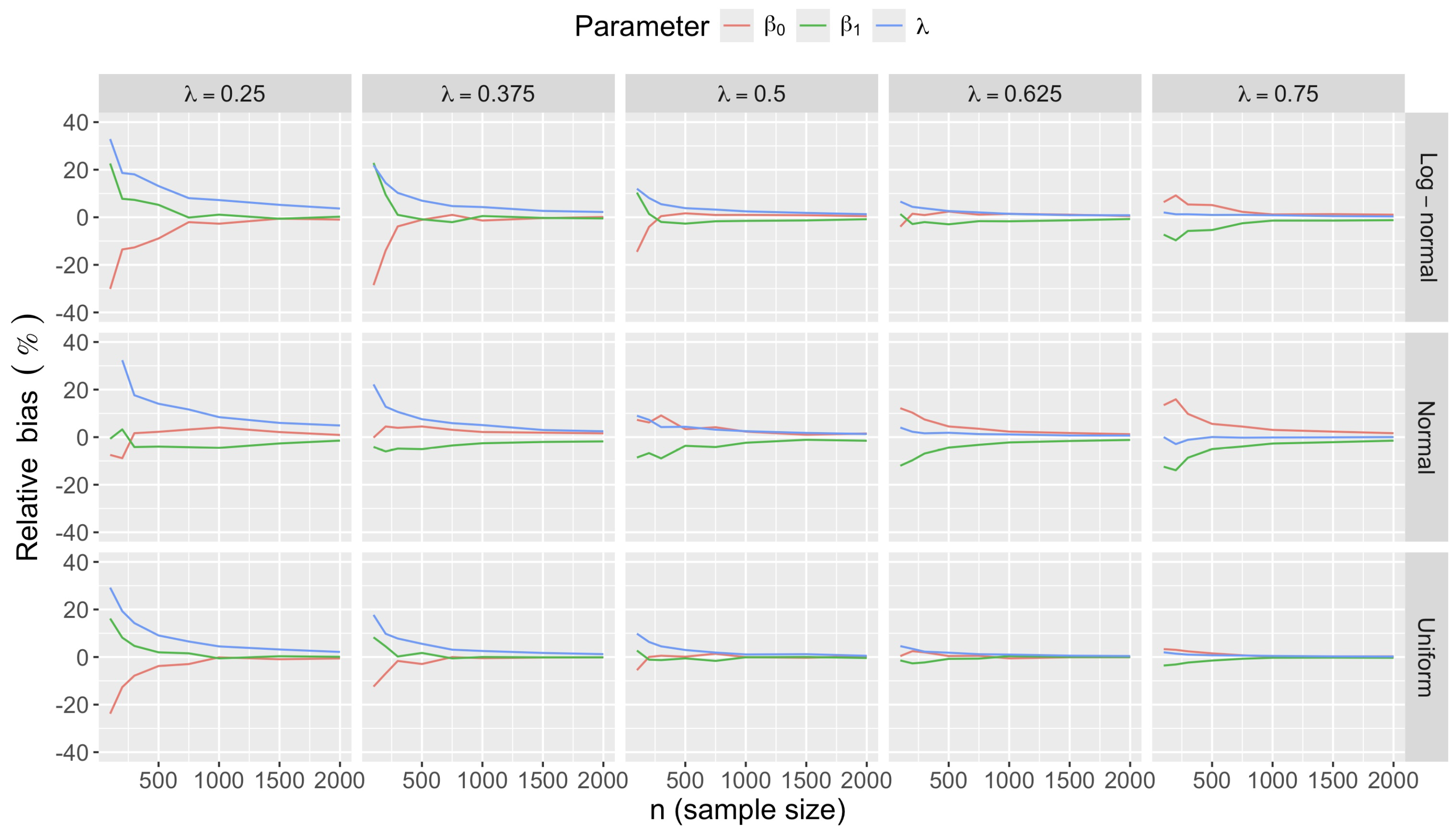
- Bias in . At , the relative of is close to zero for all considered and sample sizes . As decreases, the estimate exhibits a slight , reaching a maximum of about 10% in absolute value at when (Figure 2). We notice a pattern in the : under a uniform for instance, the is negative at and positive for . Additional simulations with values down to 0.25 (see Appendix C) reveal that under a uniform or log-normal , the in is negative (under-estimation) for high values (), essentially zero for medium values (), and positive (over-estimation) for low values (). For the normal , the pattern persists, but the is negative for .
- Accuracy of . At , the relative of is close to zero for all and sample sizes. The accuracy also decreases with (Figure 3). Indeed, under the uniform with , the of is about 6% for , but reaches about 21% for . We observe a similar trend under the log-normal , with a around 5% at , and 19% at (). The estimate is comparatively less accurate under a normal , with a around 10% at , and 25% at ().
- Bias and accuracy of and . At (all ), the of regression parameter estimates and is also close to zero (Figure 2), and the (which is then essentially the standard deviation for each estimator) is about at , at , and at (Figure 3). As decreases, the relative increases, reaching for and for when and . This indicates that the lower , the larger the sample size required to achieve the same level of accuracy for regression coefficients.
- Effect of predictor distribution. The distribution of the predictor does not affect the accuracy of the estimates and for close to one (Figure 3). But as decreases, the relative is ceteris paribus minimum under uniform and maximum under log-normal for both and . At for instance, at under a uniform predictor. In contrast, at under a log-normal predictor.
- Impact of regression coefficients. The trends in the relative and shown for and (Figure 2 and Figure 3) are similar across combinations of and . Specifically, the of the estimates and increase with , and for , the is ceteris paribus minimum under uniform and maximum under log-normal (see Appendix C).
- Beta regression on the accuracy of . To summarize the general trends for the slope estimate , we fitted a beta regression to the values of the relative of as a function of the simulation factors. Table 4 presents the results of the fit which explain about 87% of the variability in . From Table 4, we observe that the leading factors in the variations of are , and , with significant interactions. For instance, decreasing by 0.1 results on average in a 6.5% increase in under a uniform and a small sample (). Switching then to a log-normal , we have on average a 16% increase in for small values, and about a 26% increase for values close to one. Under scenarios with , we observe an average 7% decrease in as compared with .
The presence of a significant negative interaction between n and (Table 4) indicates that larger sample sizes are generally required when as compared to when . Indeed, the generally decreases with n, but the interactive effect of with the sample size n is also negative and relatively large (twice the main effect of n) as compared to the marginal effect of n (Table 4). For instance, increasing n by 100 would result in a 5.5% average decrease in if , versus a 8.3% average decrease if .
3.2.2. Sample Size Determination
The trends in the accuracy of PML estimates indicate that the sample size in an MSB design depends on . To illustrate the importance of such trends for sample size calculation when considering an MSB framework for data analysis, we run additional simulations with sample sizes up to under a uniform with true slope and intercept . Figure 4 shows for different values, the sample size n required to achieve a specified root mean square error for the estimate .
It appears that for , a sample size of about is required to achieve . Reaching the same level of accuracy with requires a sample of size . The required sample size becomes for , and reaches when . Hence, in this particular simulation setting, halving demands about six times more samples to achieve the same 10% level of accuracy. To achieve , samples are required when , when , when and when . Hence for a 5% level of accuracy, halving demands about seven times more samples.
We observe similar trends under normal and log-normal (see details in Appendix C). For instance, under the normal , to achieve , about samples are required when . With , the required sample size becomes , that is, almost eight fold increase of the sample size requirement. Under the log-normal , about samples are required to achieve when . With , the required sample size becomes , that is, 11.6 fold increase of the sample size requirement.
3.2.3. Testing for Unit Asymptote
Figure 5 shows the rejection rate of the LR test of the null hypothesis () at the significance level of 5% for true values in and regression slopes . It appears that when the TB model is the truth () and the sample size is large (), the rejection rate of the LR test is close to the nominal level of 5% (5.5% for uniform , 4.5% for normal and 4.9% for log-normal ). This shows that the LR test detects the TB model when it is the correct model and sample size is large. Interestingly, this remains true in small sample with rejection rates under 6.7% (largest value observed under log-normal with ).
For true , we observed on Figure 5 that the power of the LR test is 1 under uniform in samples of size . In smaller samples, the power decreases with decreasing sample size, but increases as the true decreases, reaching 59% at . In other words, the LR test becomes conservative in small samples. We also notice that the rejection rates are lower under normal and log-normal as compared to the uniform . Finally, the rejection rates are lower for as compared to when the deviates from uniform.
3.2.4. Statistical Inference on Regression Coefficients
We present the finite sample properties of inference based on the large sample normal approximation of the distributions of PML estimates under the MSB model. Figure 6 shows the Coverage Probability (CP) of approximate 95% confidence interval using the inverse negative Fisher information matrix as covariance matrix for PML estimates. We observed that the CP is close to the nominal level (95%) and stays above 90% when either , or the sample size is large, or the predictor distribution is uniform or normal. For a log-normal predictor however, the CP decreases with , reaching 88% at for .
Figure 7 displays the Significance Probability (SP) of the approximate 95% confidence interval. It appears that, irrespective of the and values, the significance of the slope is close to 1 for any . The intercept coefficient is more sensitive to both and sample size, the SP decreasing and reaching 0.22 under normal at .
4. Discussion
In this paper, we propose a binomial regression framework for modeling binary data arising from processes with multiplicative steps. The use of the model is prescribed when modeling a complex binary process with no data on the detailed discrete stages of the phenomenon. As soon as we have data on each specific stage, a multivariate binomial GLM [95,96] becomes more appropriate for the data analysis. We derived conditions for the identifiability of model parameters. Not surprisingly, it is sufficient that each stage has a continuous predictor only present at that stage to ensure identifiability. The maximum likelihood estimates of the MSB model parameters are asymptotically unbiased, but subject to bias in small samples. To reduce the small sample while addressing separation issues, we developed a penalized maximum likelihood estimation procedure based on Jeffreys invariant prior. We have demonstrated the use context and usefulness of the modeling framework using synthetic data on mutant protein viability (see Figure 1).
Interestingly, both the standard binomial GLM and the ZIB model are special instances of the MSB model. Indeed, though it is not usually described as based on a multiplicative risk process, the ZIB model is based on (2), but limited to . It is apparent from (2) that the overall success probability of the binary outcome can be very small. It follows that data generated from an MSB model may have a larger occurrence of zeros as compared to the corresponding standard binomial model. This observation immediately points to the ZIB model which has become popular for modeling binary data with an excess of zeros relative to the expectation under the standard binomial model [63,64,65,66]. The ZIB model stems from a mixture of two distinct subpopulations where one subpopulation is subject to a risk factor (group of “susceptible” units) whereas the other subpopulation is not (group of “immune” units). This can be mathematically described as a sequence of two Bernoulli processes. A first Bernoulli process assigns each individual to one of the two subpopulations. Then, the susceptible subpopulation, when exposed, is subject to a risk through a second Bernoulli process, while the immune subpopulation is not subject to any risk, even if exposed. The first stage of the process is considered as a source of nuisance and is not of interest to the data analysis [63]. It is here important to notice that the MSB model (8) is not a zero-inflation model. The model simply restricts the success probability of the binomial outcome to the subset of , equally allowing for inflation of both zeros and ones.
The asymptote parameter included in the MSB model (maximum success probability for the binary outcome) can capture unknown and missing stages. In particular, when only one stage is known for the process under investigation, provides an estimate of the importance of unknown or unaccounted stages or components in the determination of the binomial outcome. In health data context for instance, can represent a cure fraction [63], or a maximum survival probability. The standard binomial model would over estimate survival or risk if we omit , leading to poor prediction (Figure 1), and possibly to poor policy design. We investigated the finite sample properties of a non-standard likelihood ratio test for detecting . The test have shown rejection rates (of the assumption ) close to the nominal level when (Figure 5). The test is generally conservative and will point to only when the latter is strongly supported by the data. Hence, when studying a phenomenon without a strong justification that the process is additive, it is worthwhile testing the MSB model against the standard binomial model to identify which model is supported by the available data. Rejecting would suggest the absence of some important stages or covariates.
We investigated the finite-sample properties of the penalized maximum likelihood estimates via simulations. It turns out that affects the estimation of regression coefficients. In particular, lower values are associated with higher mean square errors in regression coefficient estimates. This implies that larger samples are required for lower values (Figure 4). Intuitively, means more failures in the binary response as compared to . However, unlike the failures under which provide as much information on regression parameters as successes, the additional failures due to do not provide any information on regression parameters. Stated otherwise, a lower means that each data point is less informative as compared to when . Hence the effective size of the sample contributing to the estimation of regression parameters is only a small proportion of n when is very low. We also established that larger sample sizes are required under log-normal distribution as compared to uniform or normal distribution of predictors.
We finally point to a few open questions that deserve attention. First, a rigorous theory of the existence, consistency and asymptotic normality of the (penalized) maximum likelihood estimators of MSB model parameters should be established. A related aspect of interest is the identifiability and inference when predictor dimension is much larger than the sample size. Second, the bias in parameters estimates relates to the particular parameterization of the MSB model. Nevertheless, first order bias corrected estimates can perform substantially better (in terms of accuracy, i.e. mean square error) than crude maximum likelihood estimates [97]. Although the use of the Jeffreys invariant prior as likelihood penalty ensures finite estimates and reduced bias, it does not completely remove first order bias from the maximum likelihood estimates of the MSB model parameters. Further bias reduction is thus possible using recent general purpose methods developed for nonlinear models (see e.g [98]). Third, diagnostic statistics such as influence measures [99] should be developed for real data analysis under the MSB model framework. Fourth, the power of the test for unit asymptote may be improved by implementing the Bartlett correction [100] for the likelihood ratio statistic. Moreover, the score test, an alternative to likelihood ratio test, may offer a faster procedure for model selection since it only requires fitting the null model (i.e. under : ) [101]. Last, but not least, we assumed that measurement error standard deviations are known in this work. Future research should investigate to what extent the proposed conjugate measurement error distribution is robust to distribution mis-specification.
Author Contributions
Conceptualization and methodology, C.T., Y.S. and C.M.; software, C.T.; resources, C.M.; writing—original draft preparation, C.T.; writing—review and editing, C.T., Y.S., and C.M.; visualization, C.T.; supervision and funding acquisition C.M.; All authors have read and agreed to the published version of the manuscript.
Funding
Research reported in this publication was supported by the National Institute Of General Medical Sciences of the National Institutes of Health under Award Number P20GM104420. The content is solely the responsibility of the authors and does not necessarily represent the official views of the National Institutes of Health.
Institutional Review Board Statement
Not applicable.
Data Availability Statement
The authors confirm that the data supporting the findings of this work are available within the article.
Acknowledgments
The authors acknowledge the support of The Institute for Interdisciplinary Data Sciences for high performance computing. They also thank Holly Wichman and other members of the Institute for Modeling Collaboration and Innovation for their ongoing support of interdisciplinary collaborations.
Conflicts of Interest
The authors declare no conflict of interest. The funders had no role in the design of the study; in the collection, analyses, or interpretation of data; in the writing of the manuscript; or in the decision to publish the results.
Appendix A. Proof of Propositions
Appendix A.1. Proof of Proposition 1
Proof.
Each factor in (4b) can be considered as the success probability of the independent Bernoulli variable associated with stage j given a covariate vector , i.e.,
From (A1), the Bernoulli variable can further be represented by truncating a continuous distribution, e.g. truncated normal, logistic or scale mixture of skew normal variables [102]. In this framework, has the stochastic representation
where means “equal in distribution to”, and H denotes the distribution with cdf h. For the logit link for instance, is the logistic distribution with mean and variance ; and in the case of the probit link, is the normal distribution with mean and variance . From Equation (6), we have . It follows that is a function of as . It then appears that the integral in (9) can be simplified by choosing the distribution of the measurement error such that the distribution of is in the same family as . Indeed, since and are independent, has variance with , and since both and have null mean, the representation (A2) becomes
In light of (A2), the distribution H in the stochastic representation must have variance in order to write e.g. . From , we get by setting :
It follows that the expectation of is given by
□
Appendix A.2. Proof of Proposition 2
To prove Proposition 2, we make use of the following two Lemmas.
Lemma A1.
Consider the function defined for as
where , is a semi-positive definite matrix, and is a positive constant. The function is injective, and accordingly, for any , the equation has a unique solution .
Proof.
Denoting the identity matrix, and setting , the Jacobian matrix of is given by . Further calculus yields
By the matrix determinant lemma [103], the determinant of is given by
Since is semi-positive definite, and for any . It follows that for all . □
Lemma A2.
Consider the function defined for and as
where with linearly independent components. The function is injective, and accordingly, for any and , the equation has a unique solution .
Proof.
The Jacobian matrix of is given by . Note that the second term in the square bracket is well defined since have linearly independent components and imply that . The determinant of is thus
It follows that for all non null . □
Proof of Proposition 2.
Let us denote the probability space on which the random vector is defined. Suppose that almost surely. Then assumptions C1 and C2 imply the existence of a positive constant such that for every , , , and , . It follows that there exists , outside the region (of measure zero) where such that given that , and . For such a , the equality reads .
For simplicity in the presentation we define so that can be rewritten as . We first show that the quantities , and are individually identifiable. In case either and are known constants in the MSB model, we only need to be identifiable. Otherwise, from or , the identifiability of or is reduced to the identifiability problem in the standard binomial regression model. Specifically, assumptions C1 and C2 ensure that and respectively imply that and (see e.g. [104]). As for , reads
where , . Set and . By the positivity of all h values under condition C2, and given that , we can write for any :
Differentiating with respect to , a continuous predictor in with regression coefficient (or ) under condition C3, we get
where (density function corresponding to the link h). The right hand side of the result is zero because the right hand side of (A7) does not depend on . The equality (A8) implies
Further differentiation of both sides of Equation (A9) with respect to gives
where the factor zero in the first term on the left hand side results from (A8), and the right hand side is zero because the left hand side of (A9) does not depend on . The last equality implies
Equations (A9) and (A10) gives the double equality
which is central to our proof of . We next consider specific cases of link functions.
-
Case of logit link:Here, , hence . Equation (A9) becomesDifferentiating both sides of the last equality with respect to yields . Along with the condition C1, this implies that , and by Lemma A1, we get .
-
Case of probit link:We have , and , hence . Note that by the condition C1 and the assumption , we have . Equation (A10) thus readsThen, because the assumption gives and condition C1 ensures , by Lemma A2, we have , which then gives by Lemma A1. We have overall shown that under the logit or probit link function, implies that for .
It remains to show that implies that , and . In case both and are known constants in the MSB model, implies that as a function of is invertible ( given that and ). Hence implies . If both and are not known constants, we have for all , (where ) which leads to by the above argument used for . In case exactly one of and is a known constant (say is a known constant), the second (say ) can be uniquely recovered from knowing and .
If none of and is a known constant, then the condition C3 ensures that there is a continuous predictor in the linear predictor of or in the linear predictor of . Then, reads . Suppose that we have , then we get and follows. This results in . Since and , it follows that . If we have , then we get giving . From and , it follows that . □
Appendix B. Score Vector and Information Matrix
Appendix B.1. Maximum Likelihood
The Fisher (expected) information matrix required in the penalized log-likelihood function (15) is defined as the variance-covariance matrix of the score vector [83]:
From (14), the score vector is given by
where is the vector of first order partial derivatives of with respect to the elements of the parameter vector . From (12), is given by:
where
with (density function corresponding to the link h),
Note that in the absence of measurement errors (), so that . Since does not depend on , and , we obtain the Fisher information matrix
When the ML estimator of exists, large sample inference on relies on the asymptotic covariance matrix as usually in GLMs. A candidate for the asymptotic covariance matrix is the inverse of the observed information matrix (evaluated at ) [105], given for the MSB model (8) by where
with . By differentiating (A12) with respect to , we obtain
where is obtained from (A13) as
where for and on setting :
An alternative to used in is the Fisher information matrix . Using , we have the potential asymptotic covariance matrix as an alternative to . For the purpose of constructing asymptotic confidence intervals for estimates, recent studies suggest that the Fisher information performs at least as well as the observed information matrix [106,107,108]. Interestingly, is also less expensive to compute as compared to . Indeed, Equation (A17) shows that even after computing the score (A12), a lot of additional computations are required to obtain . However, is usually available as a by-product from optimization routines in popular statistical softwares (see e.g. optim in R [84]).
Appendix B.2. Penalized Maximum Likelihood
For PML estimation based on (15), the penalized score is given by
where is the score given in (A12), and by the chain rule, the double score penalty satisfies
The required derivatives of are obtained from as
where is the jth element of given by Equation (A13), and the matrix has u,vth element , i.e.,
with the jth column of the hessian matrix given in Equation (A17). Note that Equation (A20) can be rewritten as
where and is the usual operator which stacks the columns of its matrix argument. Denoting ⨂ the Kronecker (direct) product, and applying Equation (2) in [109], we get
Further using Equation (1) in [109] yields
where is the commutation matrix [110] and m denotes the length of the parameter vector . Collecting the column vectors , we obtain
where is a jerk matrix defined as and given by
Solving the penalized score equation (with given by Equation (A19)) produces the PML estimates of . For large sample inference on , the Fisher information based asymptotic covariance matrix is given by . Indeed, the penalized Fisher information matrix (covariance matrix of ) is, by Equation (A11) (the same as for ), given by Equation (A15) because is equal to up to an additive constant (independent of the response Y) which does not affect covariance matrix calculation.
Appendix C. Simulation Details
Appendix C.1. Simulation Design
We consider the following extension of the MSB data generation process considered in Section 3:
In (A22), is the binary response for unit i, is an upper limit for the success probability of the binary response Y, h is the logit link function defined in (3), X denotes the explanatory variable following a predictor distribution denoted , and and are intercept and slopes.
Note that if with , then (A22) is a standard simple logistic data generation process. For and , (A22) represents a multistage process where only one stage is observed. We varied the upper limit of the success probability of the response Y from 0.5 to 1, varying regression coefficients as and , and the number n of units from 100 to 2000.
Under model (A22), the true success probability curves are shown in Figure A1 for , and selected values from 0.1 to 1. For a predictor X, we first considered a uniform distribution. For instance, with and , we simulated X values uniformly from the interval (Figure A2), having expectation and standard deviation , and spanning 99% probability mass of the standard logistic distribution centered at 3.
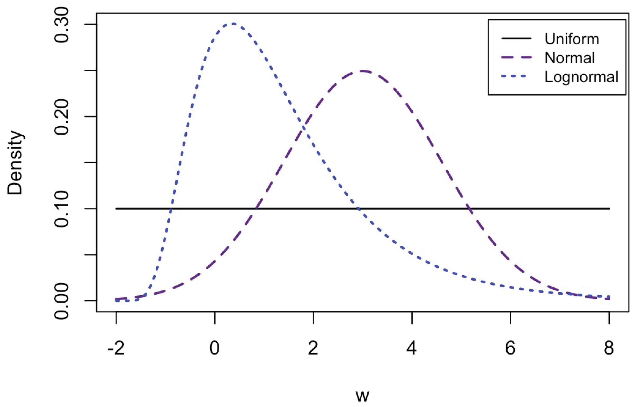
It is well established that the distribution of the explanatory variable has a large impact on inference in logistic regression [111]. To investigate this effect in our MSB framework, we considered two alternative continuous probability distributions for X, including the normal (symmetric) and the lognormal (asymmetric) distributions. Normal covariate values were simulated with mean and standard deviation . We used a shifted lognormal distribution, obtained by subtracting two from log normal variates with mean and standard deviation (log scale mean and standard are 1.1 and 0.5, respectively). For both normal and lognormal covariates, the chosen distribution parameters ensure that X values cover the interval with probability 99% when and (Figure A2). The lognormal distribution giving more weight to X values along the asymptote of the success probability curve (; Figure A2) is expected to result in more precise (lower variance) estimates of the asymptote (irrespective of the true value), but less accurate (more biased/less precise) estimates of and when the true value is low.
A summary of our simulation factors, including , , , , and sample size (n) is shown in Table A1. As performance measures, we computed the relative bias and root mean square error () of the estimates of model parameters , and , and the and of predicted success probabilities as defined in Section 3.1, based on 2000 independent replicates of each simulation setting.

Table A1.
Levels of simulation factors
| Simulation factor | Notation | Levels |
|---|---|---|
| Sample size | 100, 200, 300, 500, 750, 1000, 1500, 2000 | |
| Upper limit of success probability | 0.5, 0.75, 0.9, 1 | |
| Intercept | 3, 8 | |
| Slope | -3, -2, -1 | |
| Distribution of the predictor | Uniform, Normal, Log-normal |
Figure A1.
Success probability from model (A22) as a function the explanatory variable X for selected asymptote values and and .
Figure A1.
Success probability from model (A22) as a function the explanatory variable X for selected asymptote values and and .
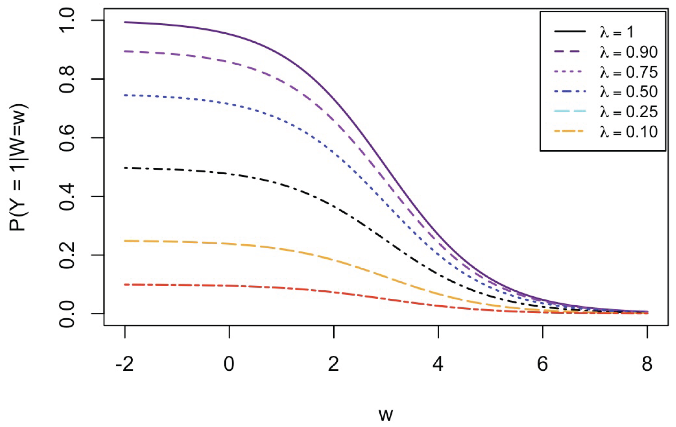
Figure A2.
Probability distributions considered for the covariate X in model (A22) with and . All density curves cover the region with probability 99% or more (100% for the uniform distribution). The normal density is above the uniform density curve over the region where the normal has 90% probability against 43% for the uniform. The lognormal density is above the uniform density curve over the region where the lognormal has 81% probability against 38% for the uniform. For general and values, X is rescaled (linear transformation) so as to preserve the logit scale range of the linear predictor .
Appendix C.2. Additional Simulation Results
Appendix C.2.1. Bias
Figure A3–Figure A14 present the relative bias in the estimates , and for model parameters , and and sample size . The relative bias generally approaches zero as n increases. For , the bias is generally negative for high true values (close to one), and positive for low values ().
Figure A3.
Relative bias of Penalized Maximum Likelihood estimates of multistage binomial model parameters , and under the MSB model data generation process in Equation (A22) with , , and .
Figure A3.
Relative bias of Penalized Maximum Likelihood estimates of multistage binomial model parameters , and under the MSB model data generation process in Equation (A22) with , , and .
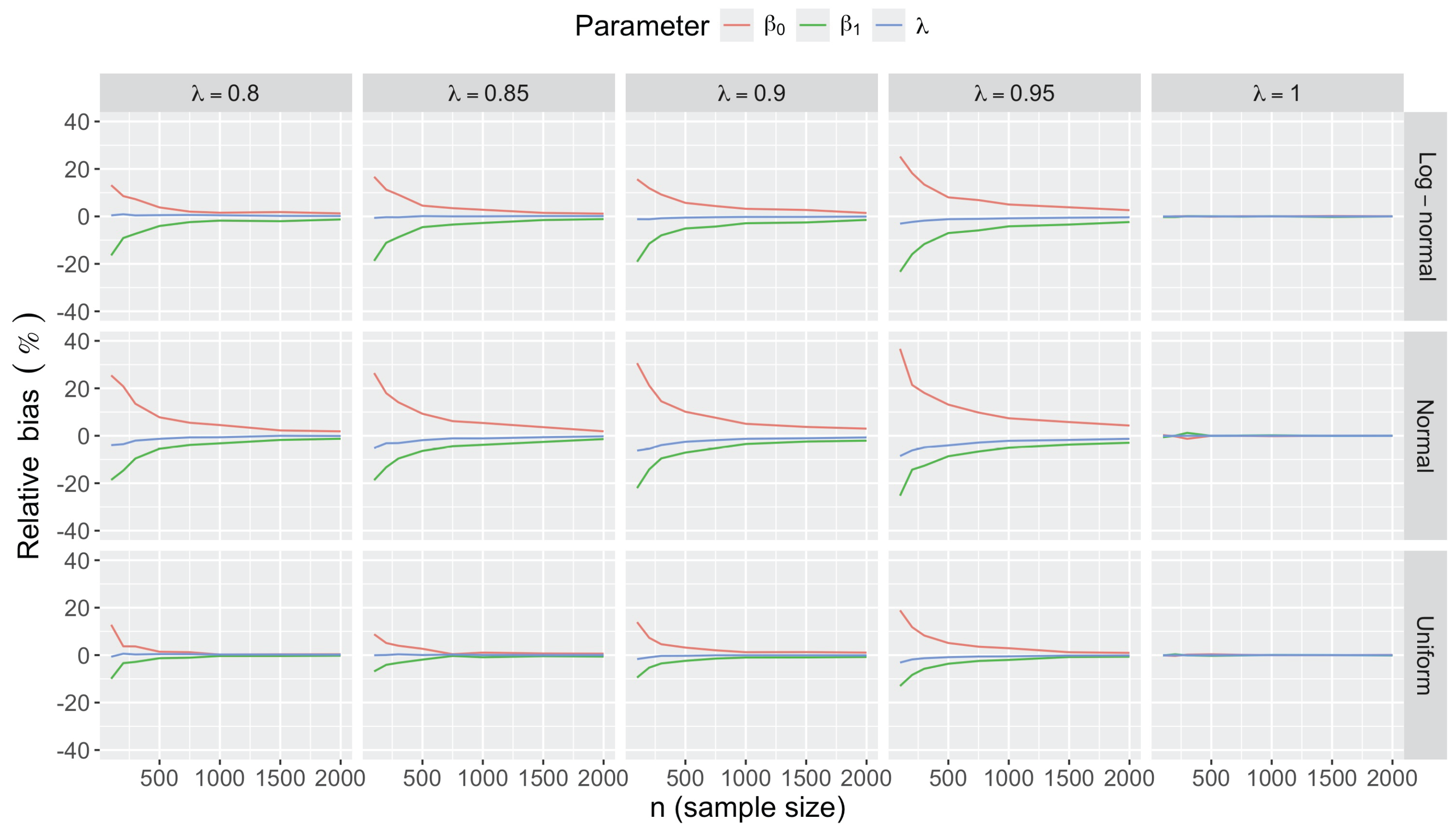
Figure A4.
Relative bias of Penalized Maximum Likelihood estimates of multistage binomial model parameters , and under the MSB model data generation process in Equation (A22) with , , and .
Figure A4.
Relative bias of Penalized Maximum Likelihood estimates of multistage binomial model parameters , and under the MSB model data generation process in Equation (A22) with , , and .
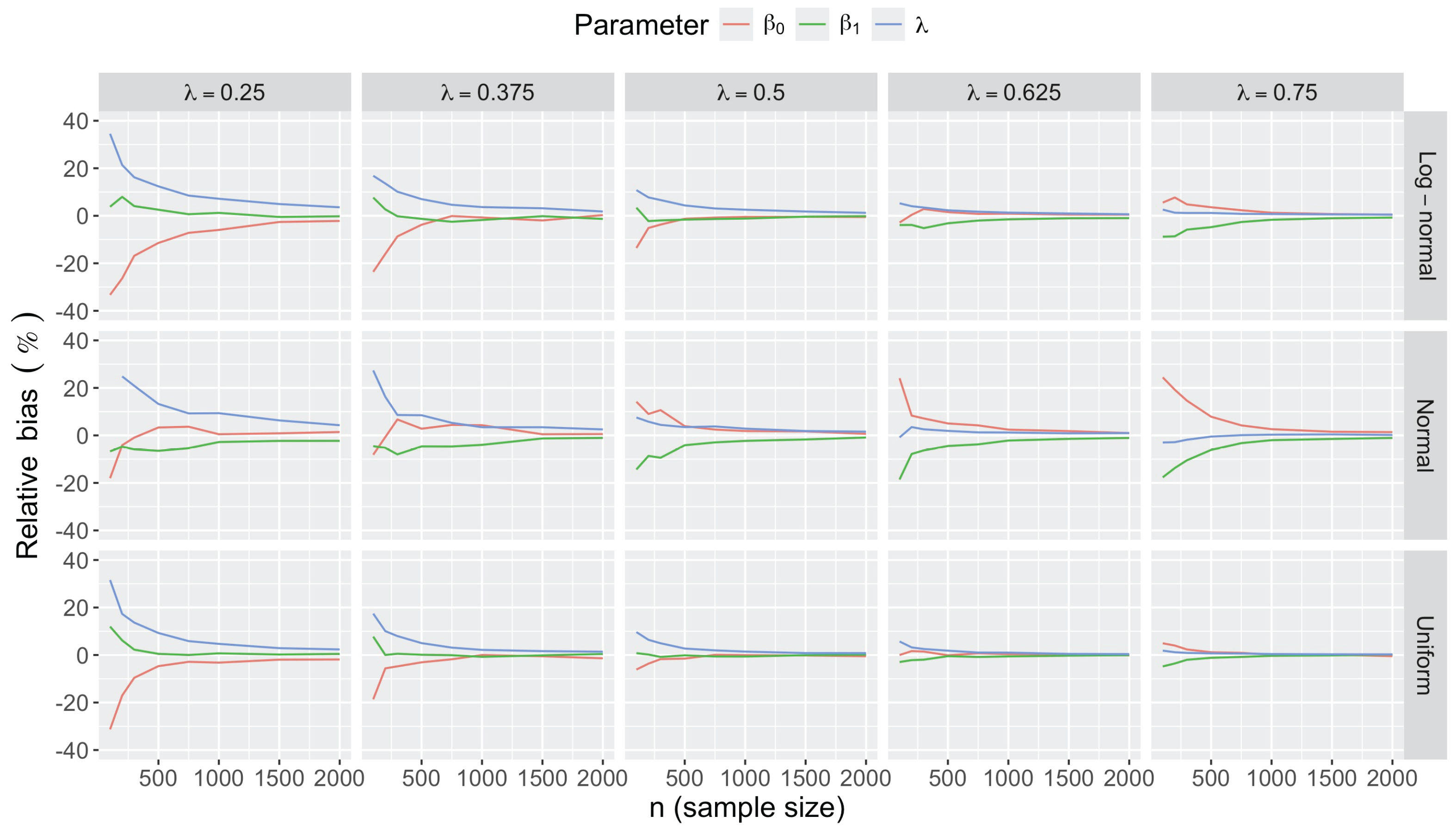
Figure A5.
Relative bias of Penalized Maximum Likelihood estimates of multistage binomial model parameters , and under the MSB model data generation process in Equation (A22) with , , and .
Figure A5.
Relative bias of Penalized Maximum Likelihood estimates of multistage binomial model parameters , and under the MSB model data generation process in Equation (A22) with , , and .
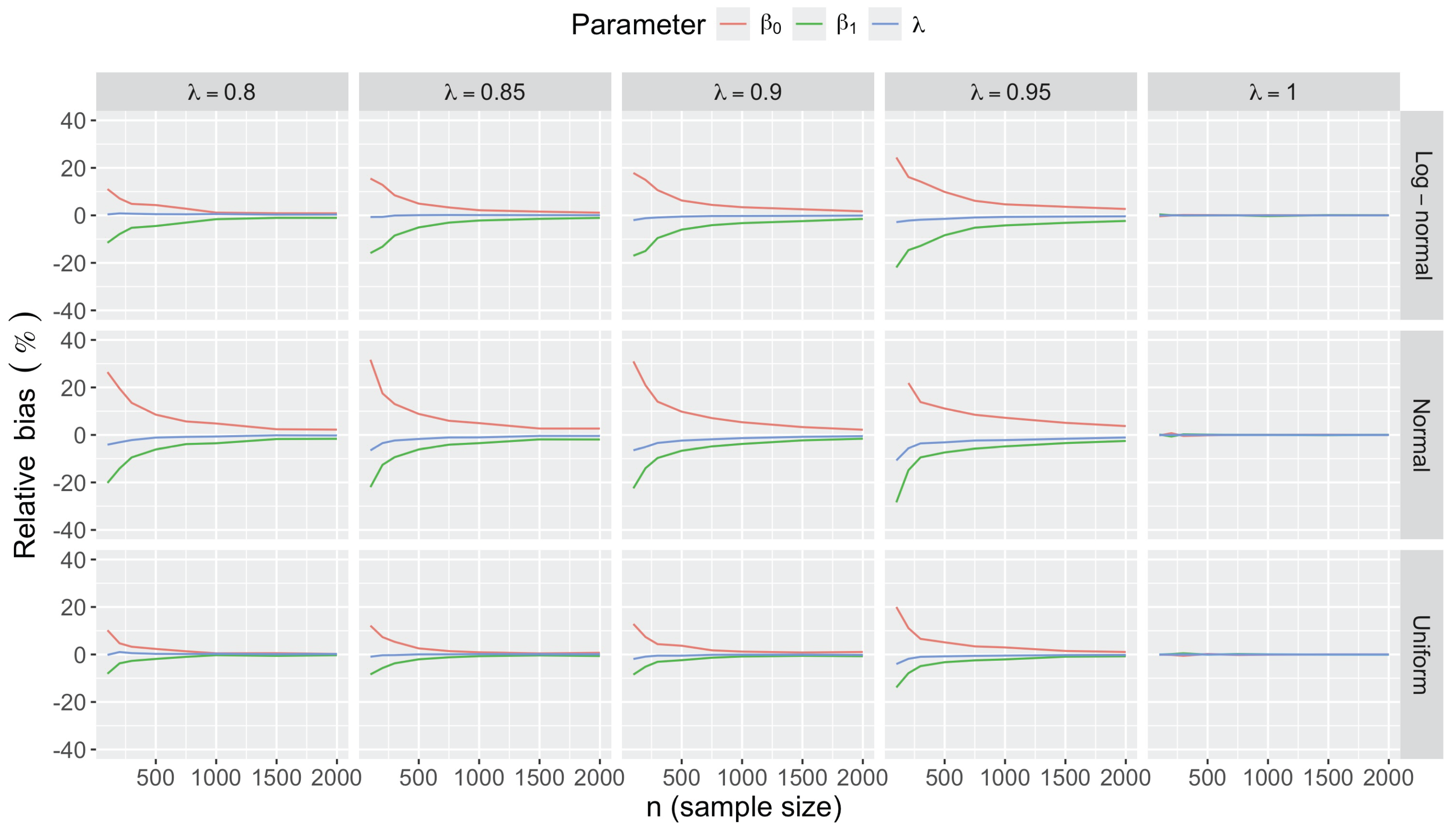
Figure A6.
Relative bias of Penalized Maximum Likelihood estimates of multistage binomial model parameters , and under the MSB model data generation process in Equation (A22) with , , and .
Figure A6.
Relative bias of Penalized Maximum Likelihood estimates of multistage binomial model parameters , and under the MSB model data generation process in Equation (A22) with , , and .
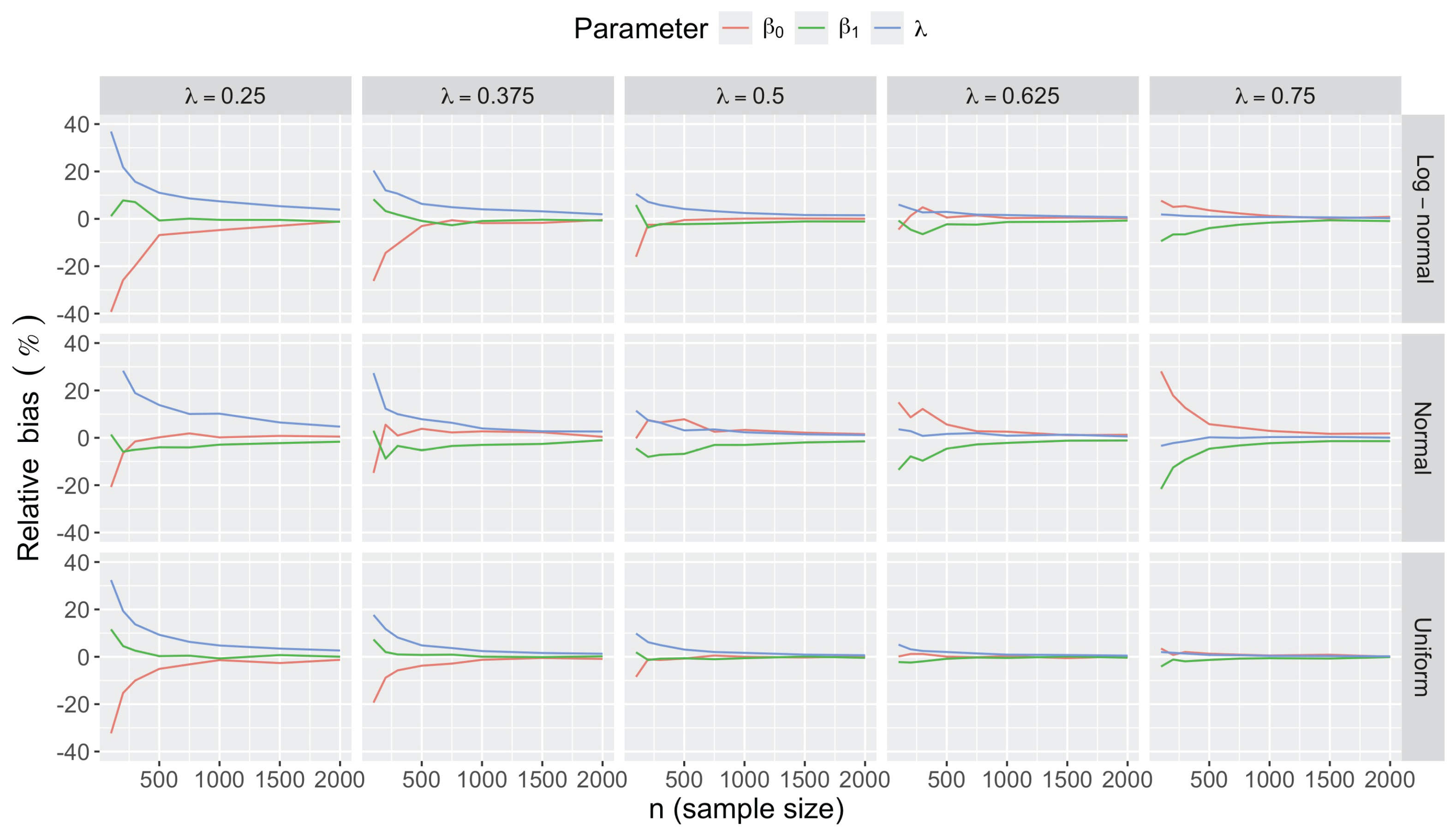
Figure A7.
Relative bias of Penalized Maximum Likelihood estimates of multistage binomial model parameters , and under the MSB model data generation process in Equation (A22) with , , and .
Figure A7.
Relative bias of Penalized Maximum Likelihood estimates of multistage binomial model parameters , and under the MSB model data generation process in Equation (A22) with , , and .
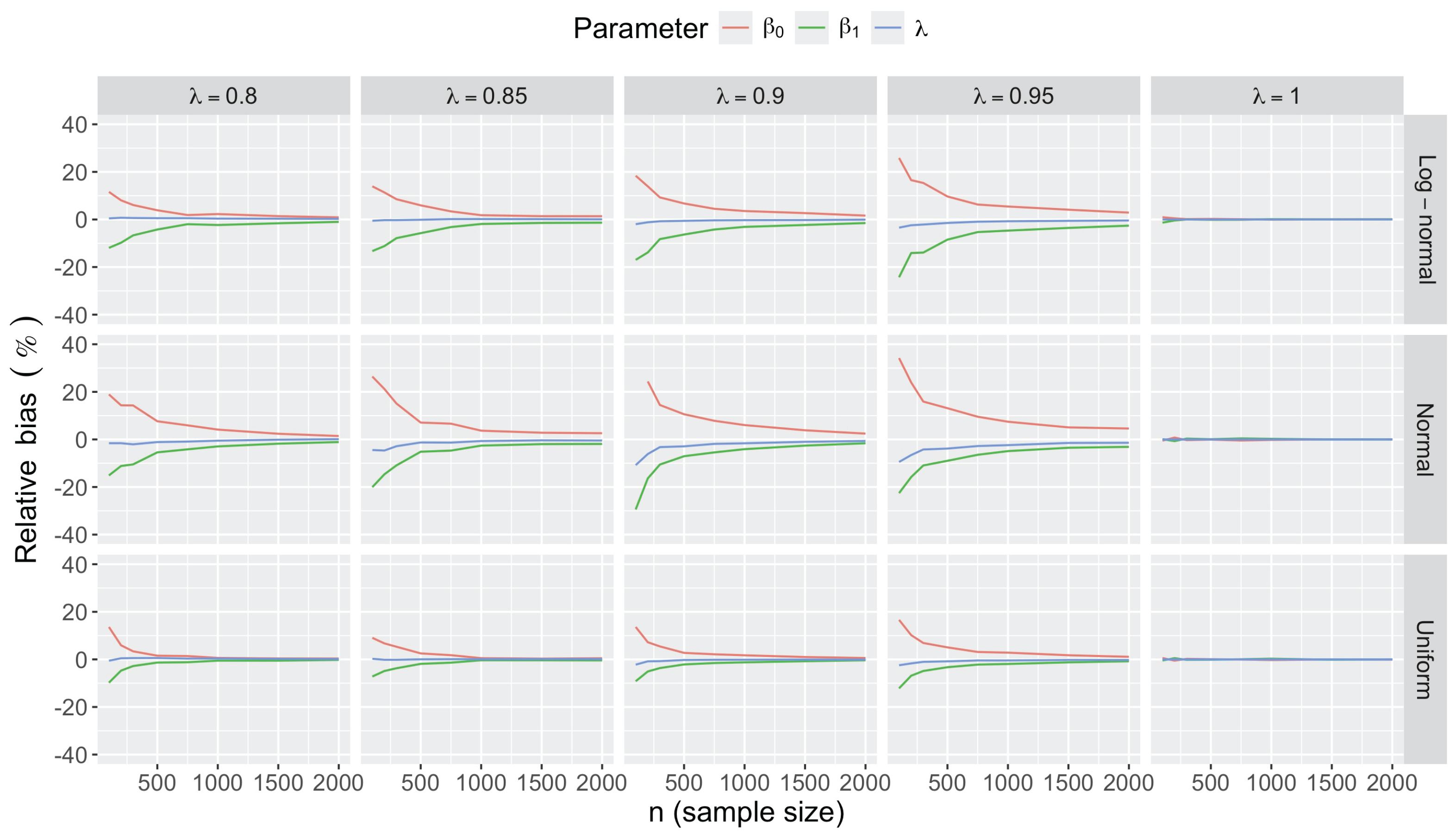
Figure A8.
Relative bias of Penalized Maximum Likelihood estimates of multistage binomial model parameters , and under the MSB model data generation process in Equation (A22) with , , and .
Figure A8.
Relative bias of Penalized Maximum Likelihood estimates of multistage binomial model parameters , and under the MSB model data generation process in Equation (A22) with , , and .
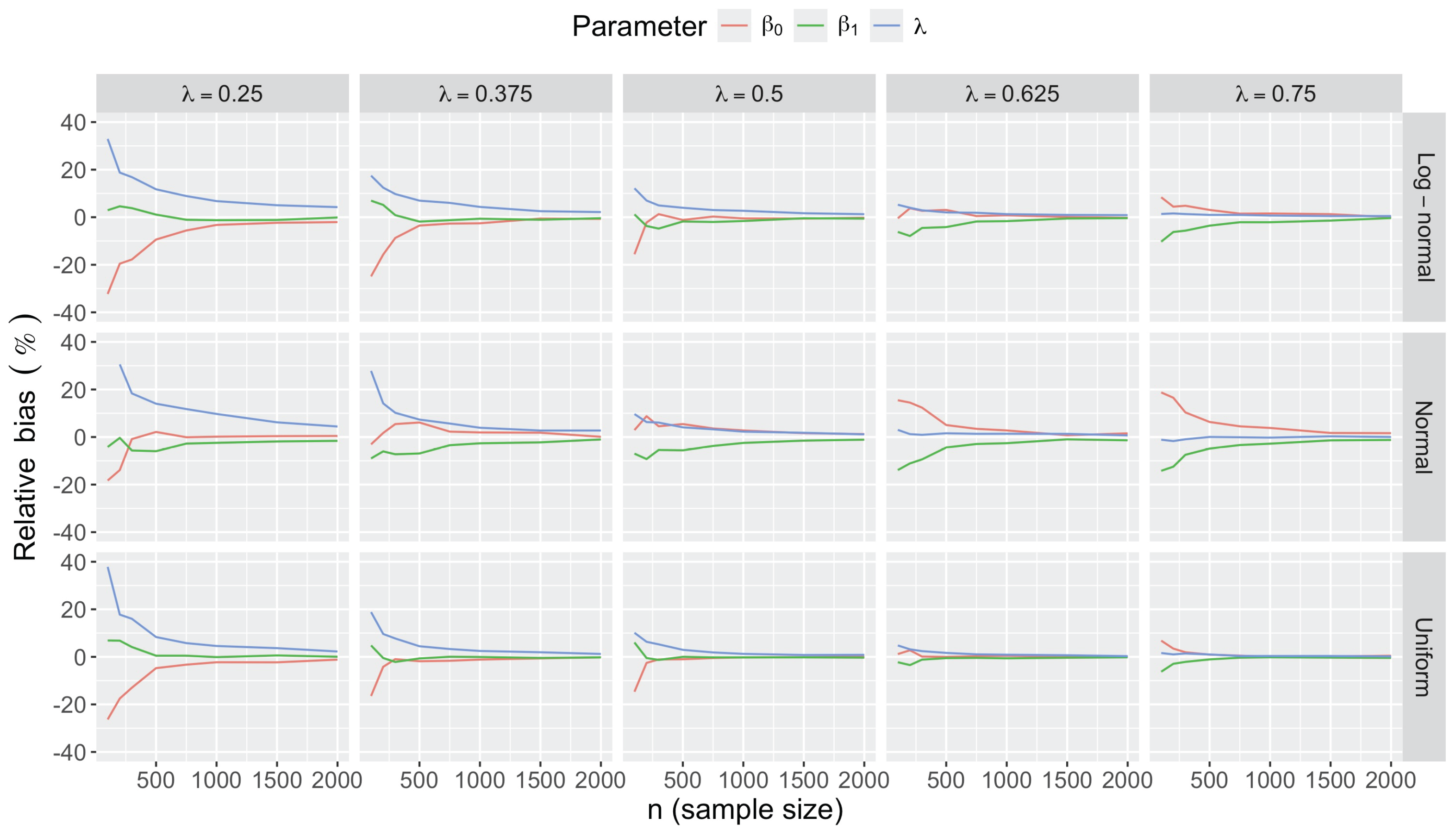
Figure A9.
Relative bias of Penalized Maximum Likelihood estimates of multistage binomial model parameters , and under the MSB model data generation process in Equation (A22) with , , and .
Figure A9.
Relative bias of Penalized Maximum Likelihood estimates of multistage binomial model parameters , and under the MSB model data generation process in Equation (A22) with , , and .
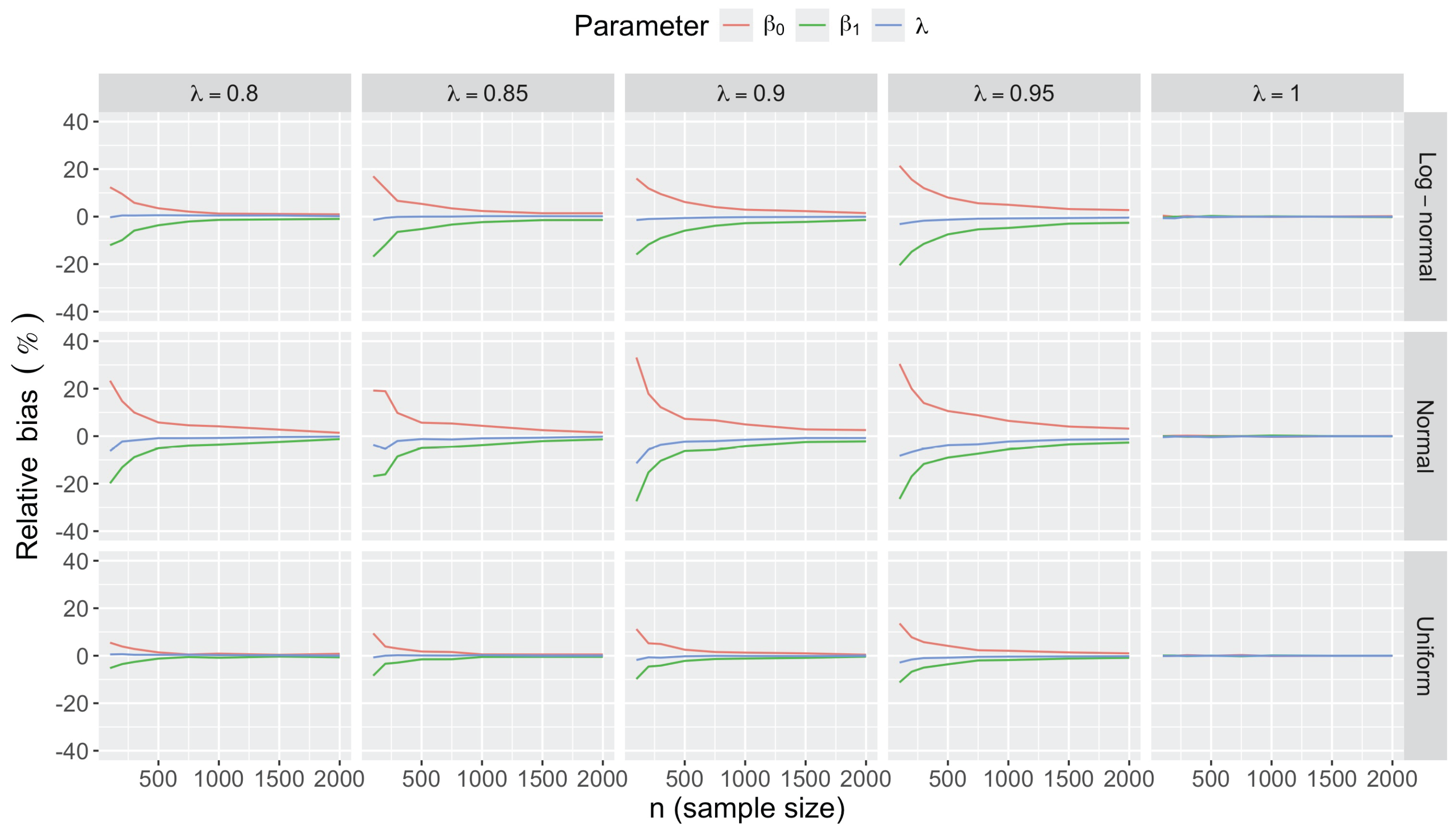
Figure A10.
Relative bias of Penalized Maximum Likelihood estimates of multistage binomial model parameters , and under the MSB model data generation process in Equation (A22) with , , and .
Figure A10.
Relative bias of Penalized Maximum Likelihood estimates of multistage binomial model parameters , and under the MSB model data generation process in Equation (A22) with , , and .
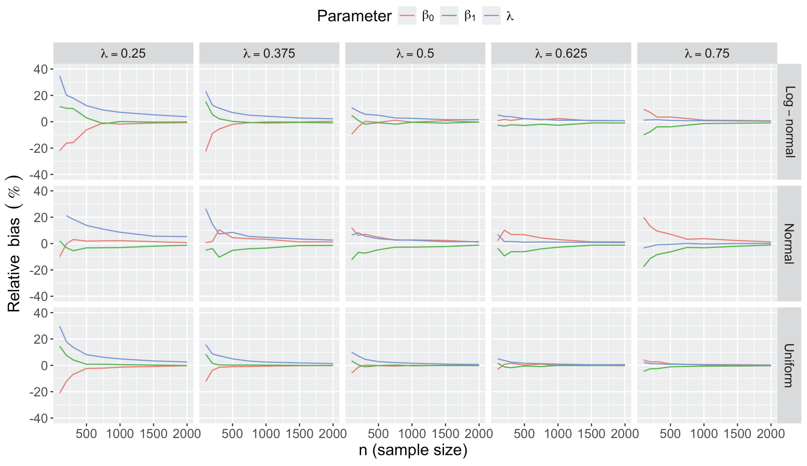
Figure A11.
Relative bias of Penalized Maximum Likelihood estimates of multistage binomial model parameters , and under the MSB model data generation process in Equation (A22) with , , and .
Figure A11.
Relative bias of Penalized Maximum Likelihood estimates of multistage binomial model parameters , and under the MSB model data generation process in Equation (A22) with , , and .
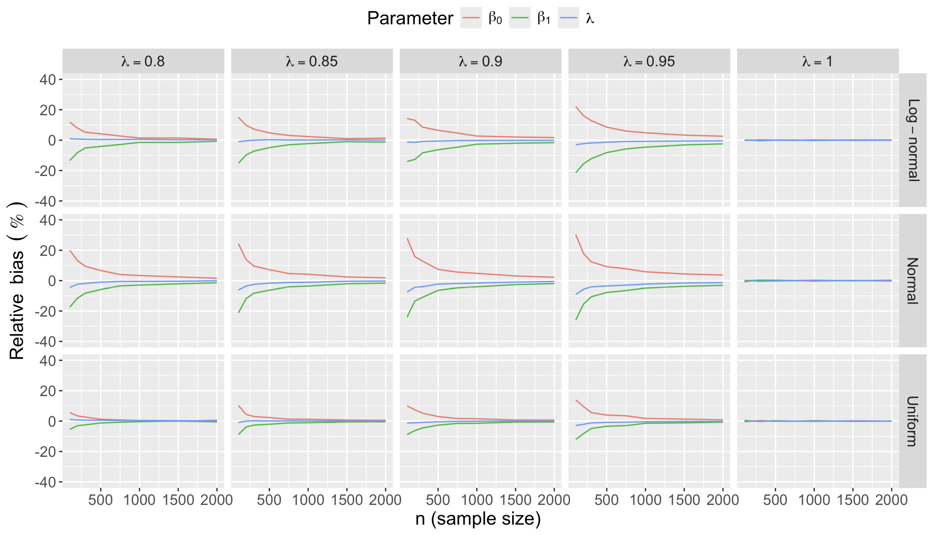
Figure A12.
Relative bias of Penalized Maximum Likelihood estimates of multistage binomial model parameters , and under the MSB model data generation process in Equation (A22) with , , and .
Figure A12.
Relative bias of Penalized Maximum Likelihood estimates of multistage binomial model parameters , and under the MSB model data generation process in Equation (A22) with , , and .
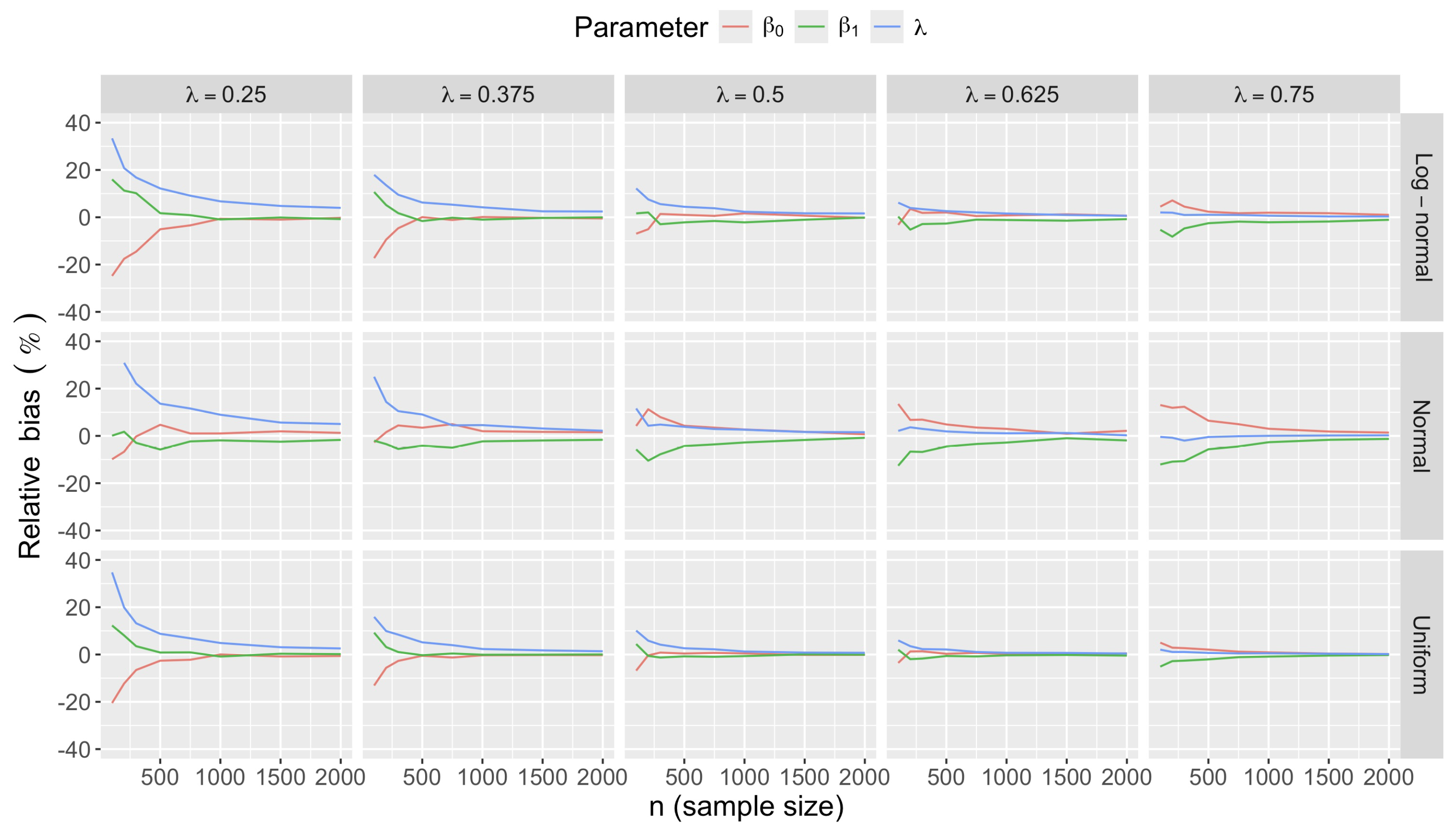
Figure A13.
Relative bias of Penalized Maximum Likelihood estimates of multistage binomial model parameters , and under the MSB model data generation process in Equation (A22) with , , and .
Figure A13.
Relative bias of Penalized Maximum Likelihood estimates of multistage binomial model parameters , and under the MSB model data generation process in Equation (A22) with , , and .
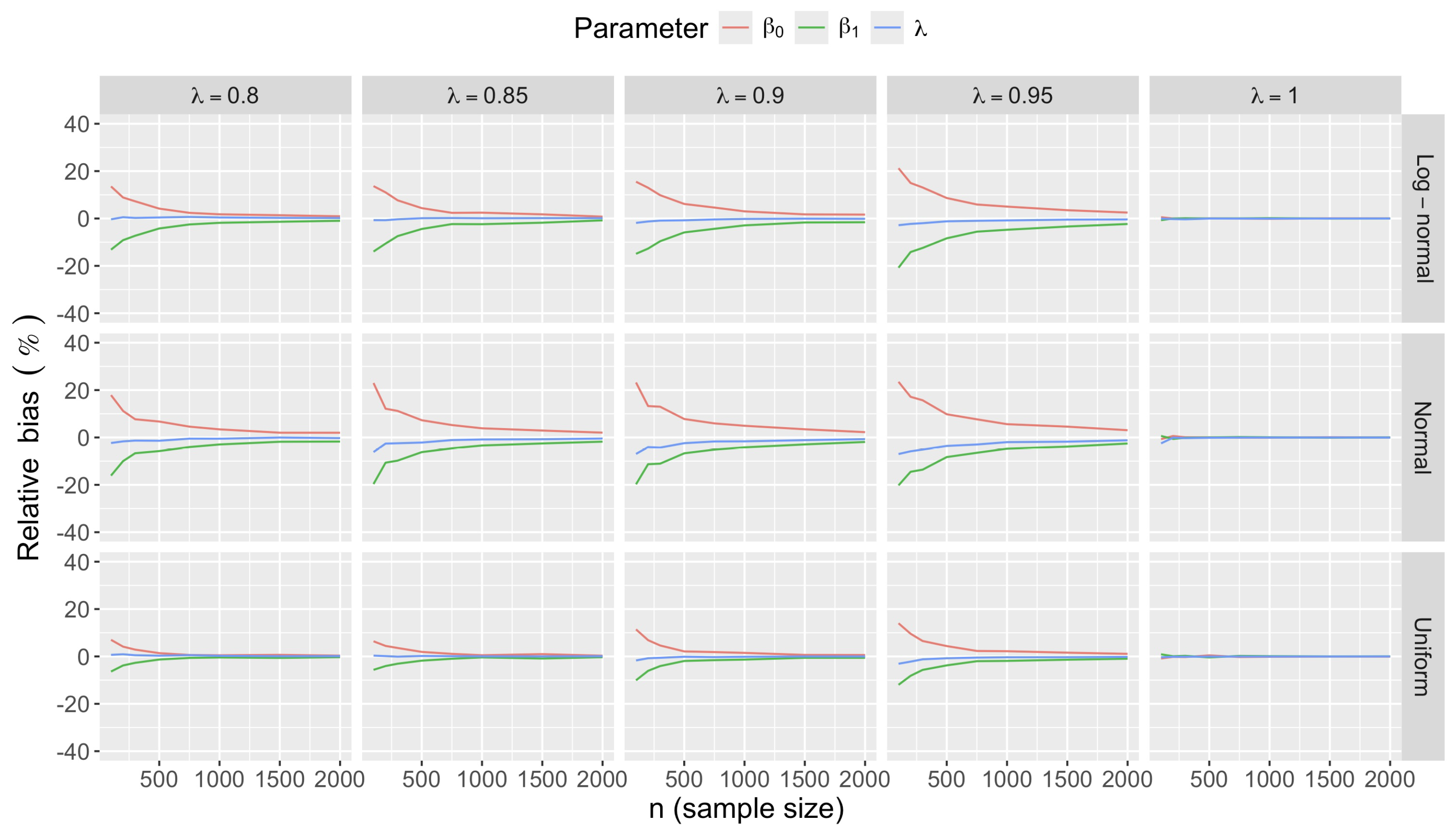
Figure A14.
Relative bias of Penalized Maximum Likelihood estimates of multistage binomial model parameters , and under the MSB model data generation process in Equation (A22) with , , and .
Figure A14.
Relative bias of Penalized Maximum Likelihood estimates of multistage binomial model parameters , and under the MSB model data generation process in Equation (A22) with , , and .
Appendix C.2.2. Accuracy
Figure A15–Figure A26 present the relative root mean square error () in the estimates , and for model parameters , and and sample size . Figure A27 and Figure A28 shows the in grouped for all parameter settings. The generally approaches zero as n increases.
Figure A15.
Relative root mean square error () of Penalized Maximum Likelihood estimates of multistage binomial model parameters , and under the MSB model data generation process in Equation (A22) with , , and .
Figure A15.
Relative root mean square error () of Penalized Maximum Likelihood estimates of multistage binomial model parameters , and under the MSB model data generation process in Equation (A22) with , , and .
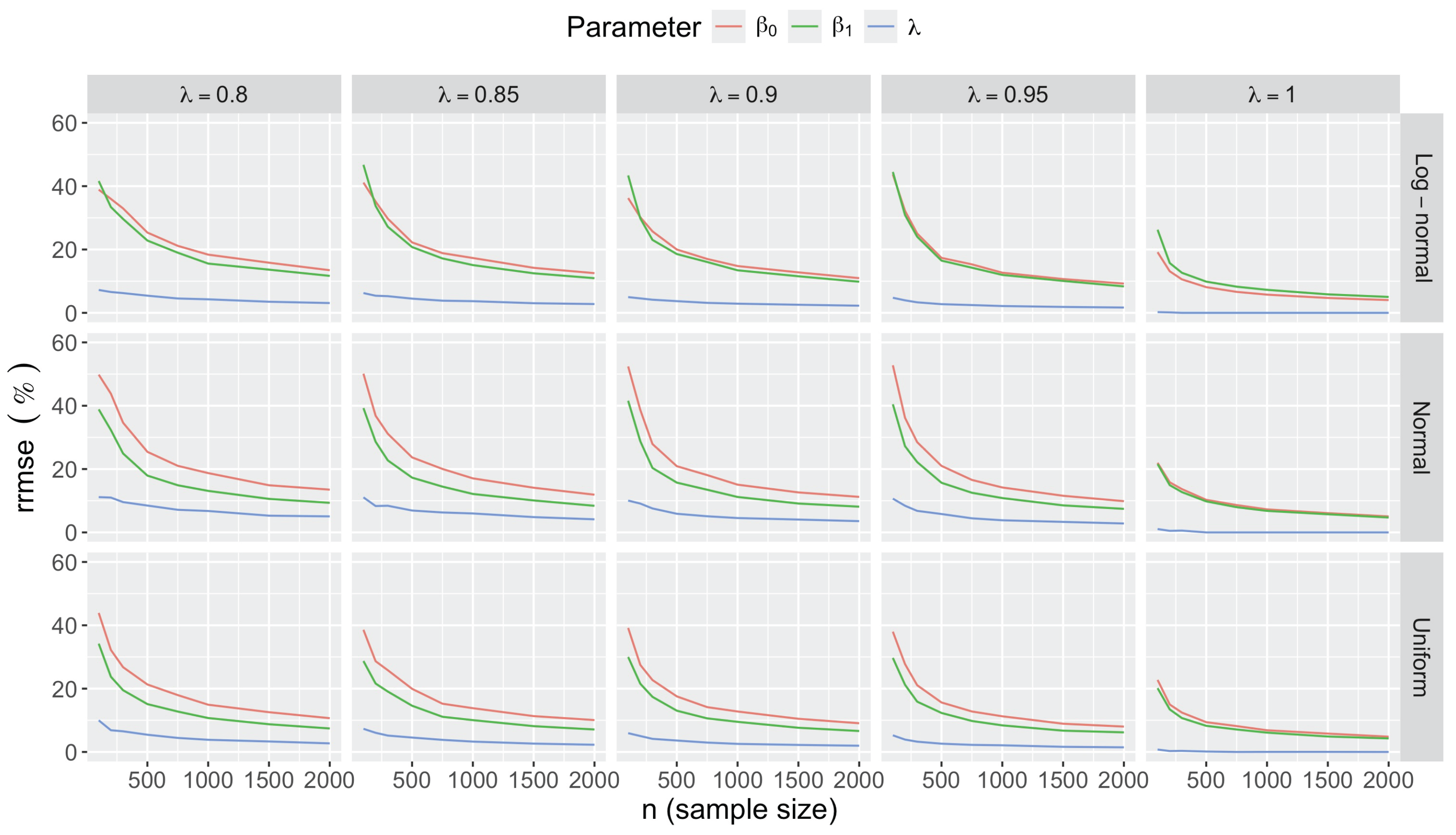
Figure A16.
Relative root mean square error () of Penalized Maximum Likelihood estimates of multistage binomial model parameters , and under the MSB model data generation process in Equation (A22) with , , and .
Figure A16.
Relative root mean square error () of Penalized Maximum Likelihood estimates of multistage binomial model parameters , and under the MSB model data generation process in Equation (A22) with , , and .
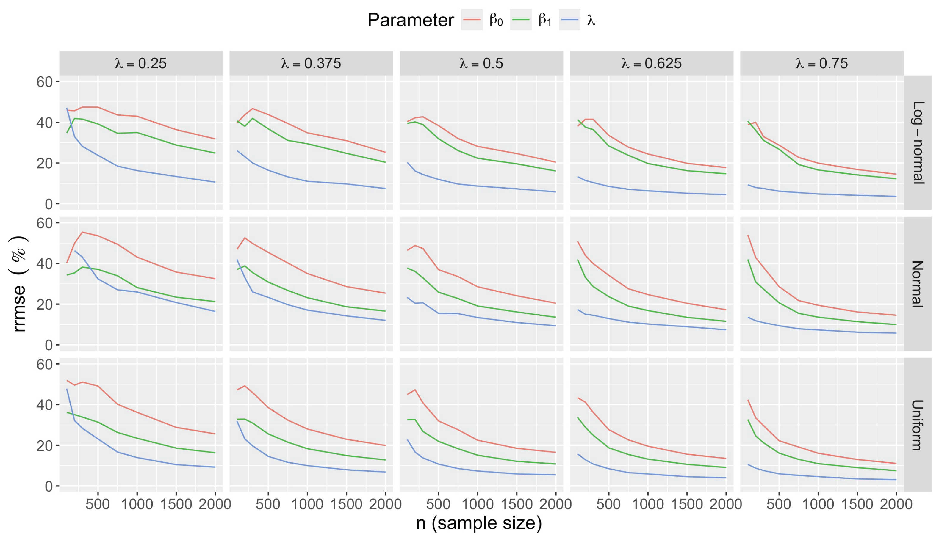
Figure A17.
Relative root mean square error () of Penalized Maximum Likelihood estimates of multistage binomial model parameters , and under the MSB model data generation process in Equation (A22) with , , and .
Figure A17.
Relative root mean square error () of Penalized Maximum Likelihood estimates of multistage binomial model parameters , and under the MSB model data generation process in Equation (A22) with , , and .
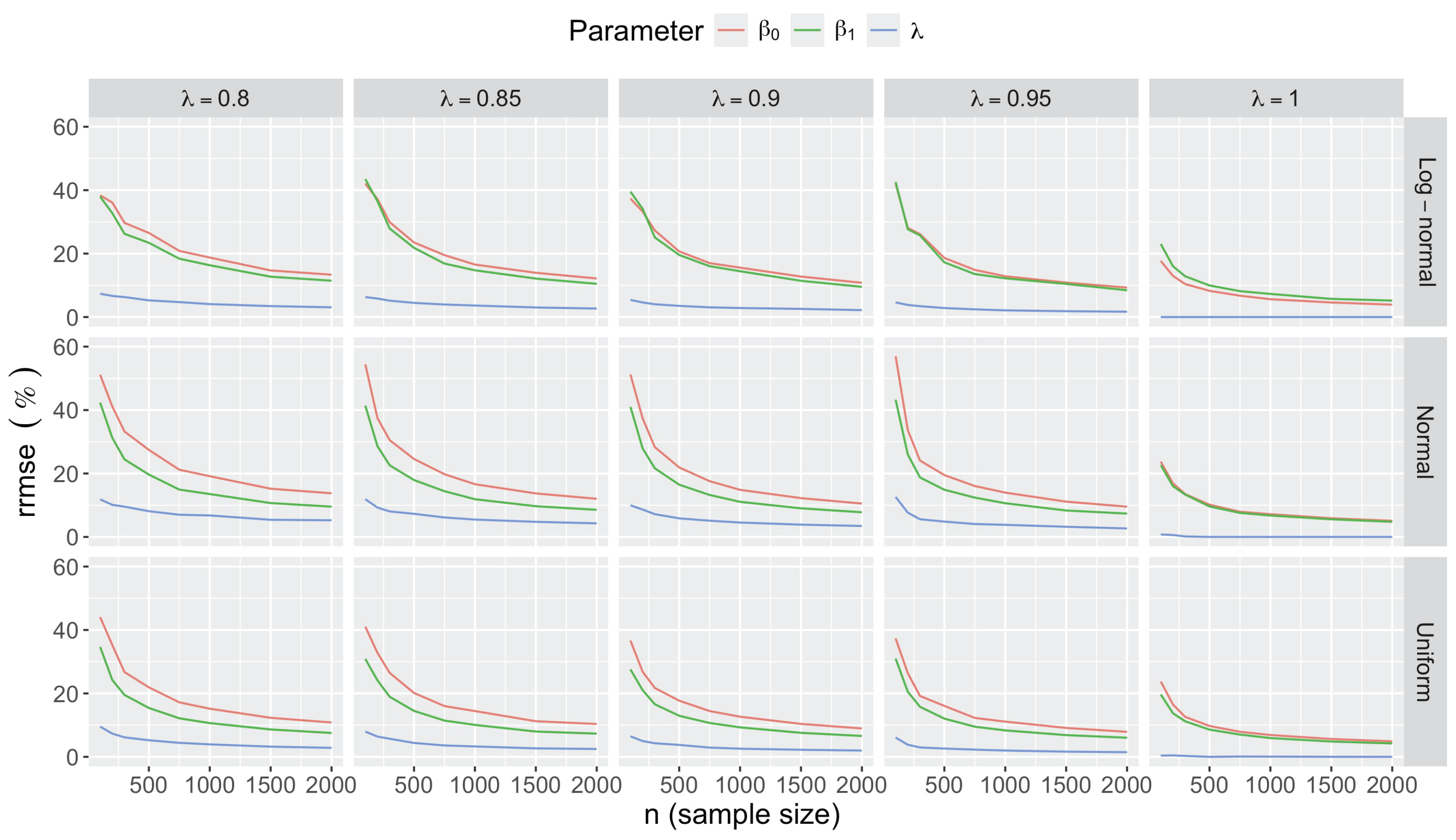
Figure A18.
Relative root mean square error () of Penalized Maximum Likelihood estimates of multistage binomial model parameters , and under the MSB model data generation process in Equation (A22) with , , and .
Figure A18.
Relative root mean square error () of Penalized Maximum Likelihood estimates of multistage binomial model parameters , and under the MSB model data generation process in Equation (A22) with , , and .
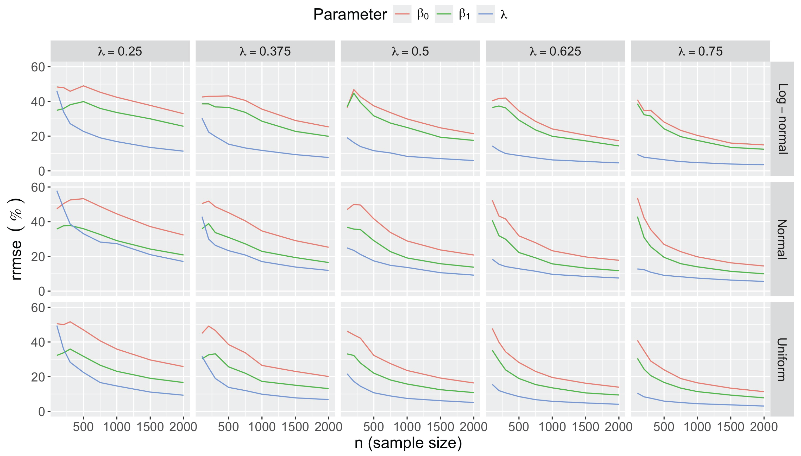
Figure A19.
Relative root mean square error () of Penalized Maximum Likelihood estimates of multistage binomial model parameters , and under the MSB model data generation process in Equation (A22) with , , and .
Figure A19.
Relative root mean square error () of Penalized Maximum Likelihood estimates of multistage binomial model parameters , and under the MSB model data generation process in Equation (A22) with , , and .
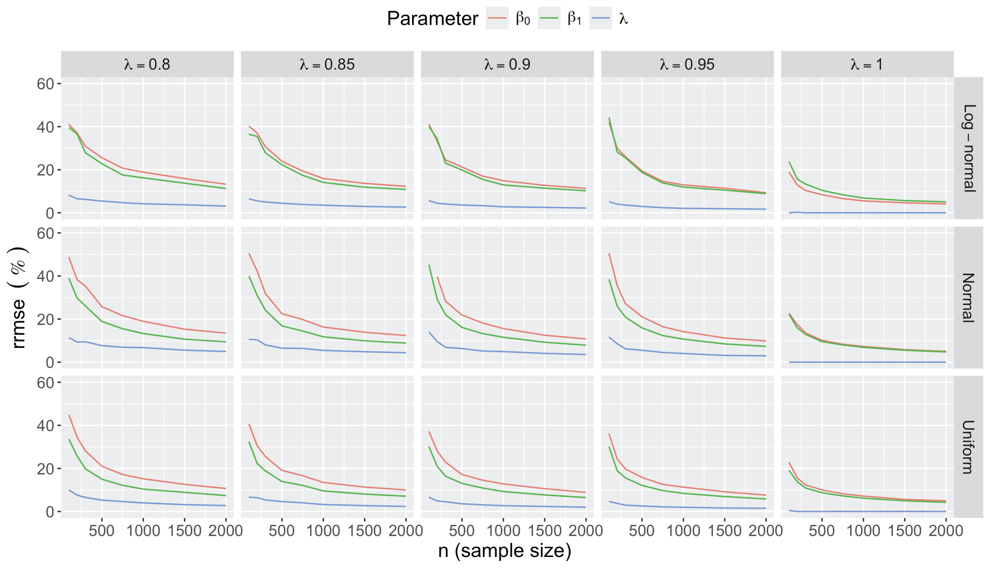
Figure A20.
Relative root mean square error () of Penalized Maximum Likelihood estimates of multistage binomial model parameters , and under the MSB model data generation process in Equation (A22) with , , and .
Figure A20.
Relative root mean square error () of Penalized Maximum Likelihood estimates of multistage binomial model parameters , and under the MSB model data generation process in Equation (A22) with , , and .
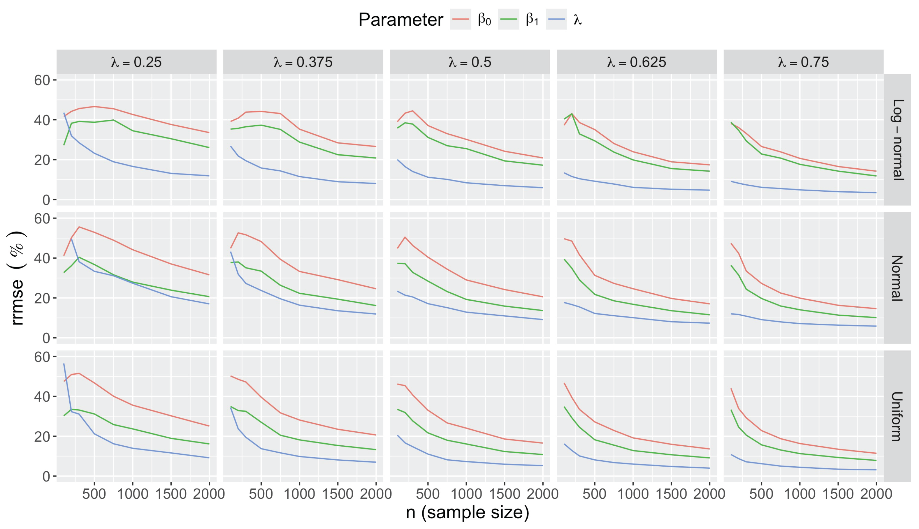
Figure A21.
Relative root mean square error () of Penalized Maximum Likelihood estimates of multistage binomial model parameters , and under the MSB model data generation process in Equation (A22) with , , and .
Figure A21.
Relative root mean square error () of Penalized Maximum Likelihood estimates of multistage binomial model parameters , and under the MSB model data generation process in Equation (A22) with , , and .
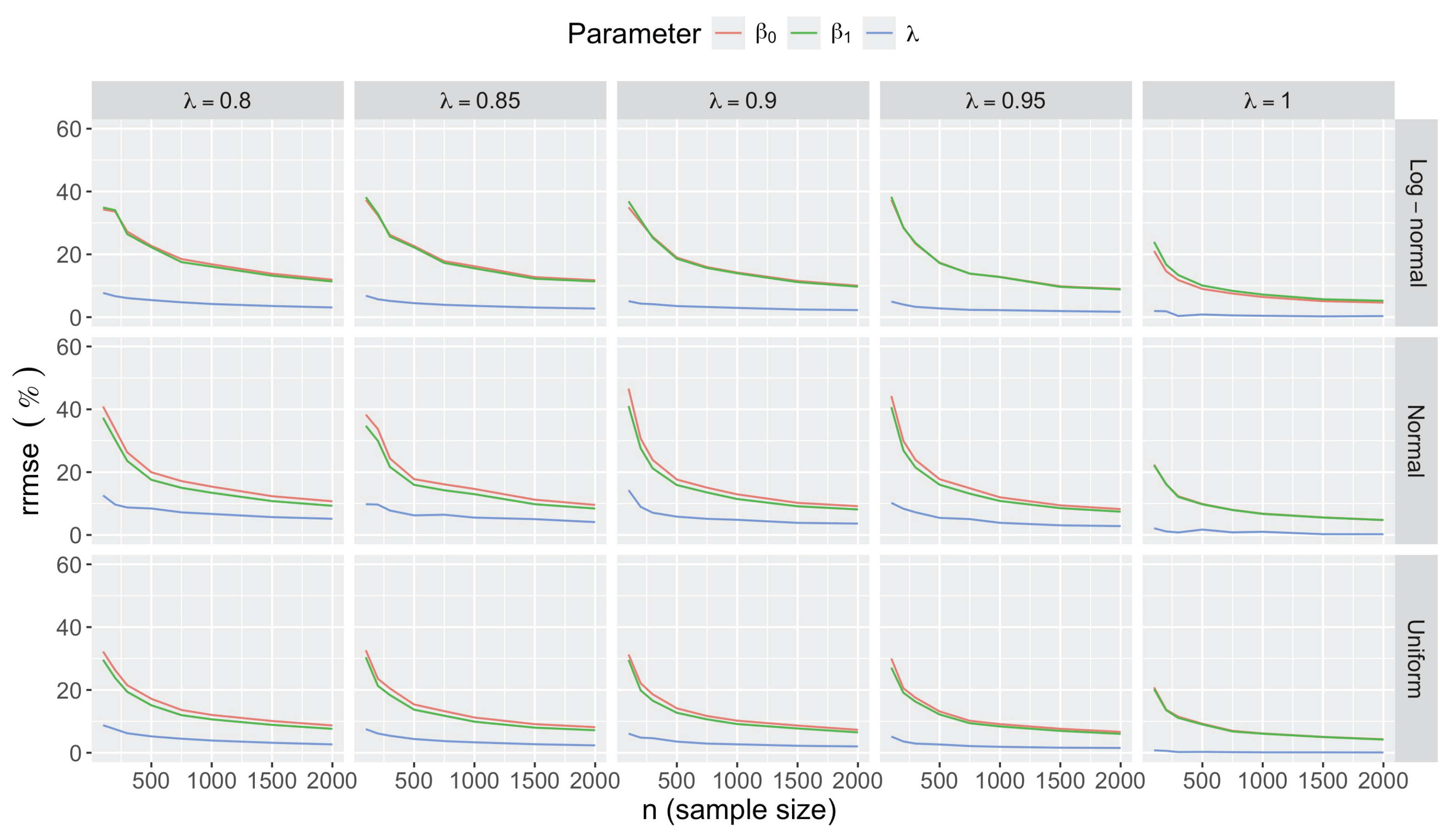
Figure A22.
Relative root mean square error () of Penalized Maximum Likelihood estimates of multistage binomial model parameters , and under the MSB model data generation process in Equation (A22) with , , and .
Figure A22.
Relative root mean square error () of Penalized Maximum Likelihood estimates of multistage binomial model parameters , and under the MSB model data generation process in Equation (A22) with , , and .
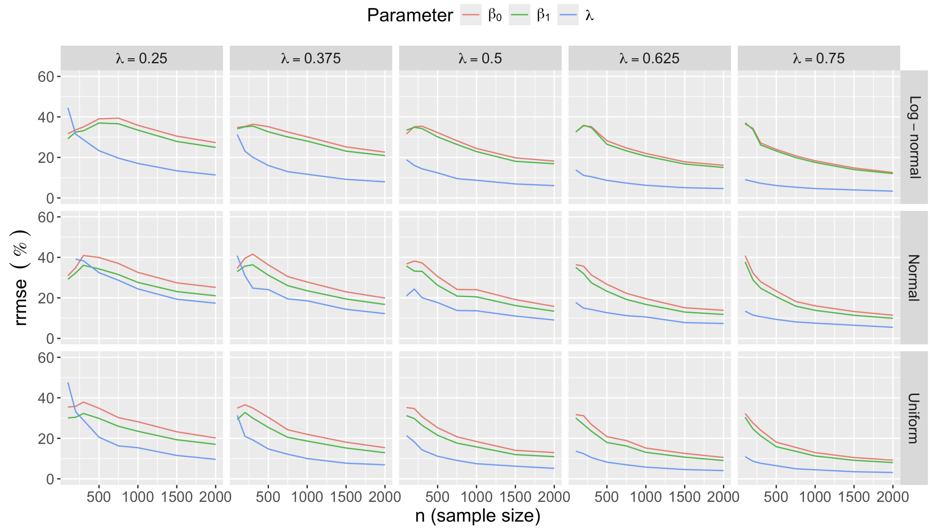
Figure A23.
Relative root mean square error () of Penalized Maximum Likelihood estimates of multistage binomial model parameters , and under the MSB model data generation process in Equation (A22) with , , and .
Figure A23.
Relative root mean square error () of Penalized Maximum Likelihood estimates of multistage binomial model parameters , and under the MSB model data generation process in Equation (A22) with , , and .
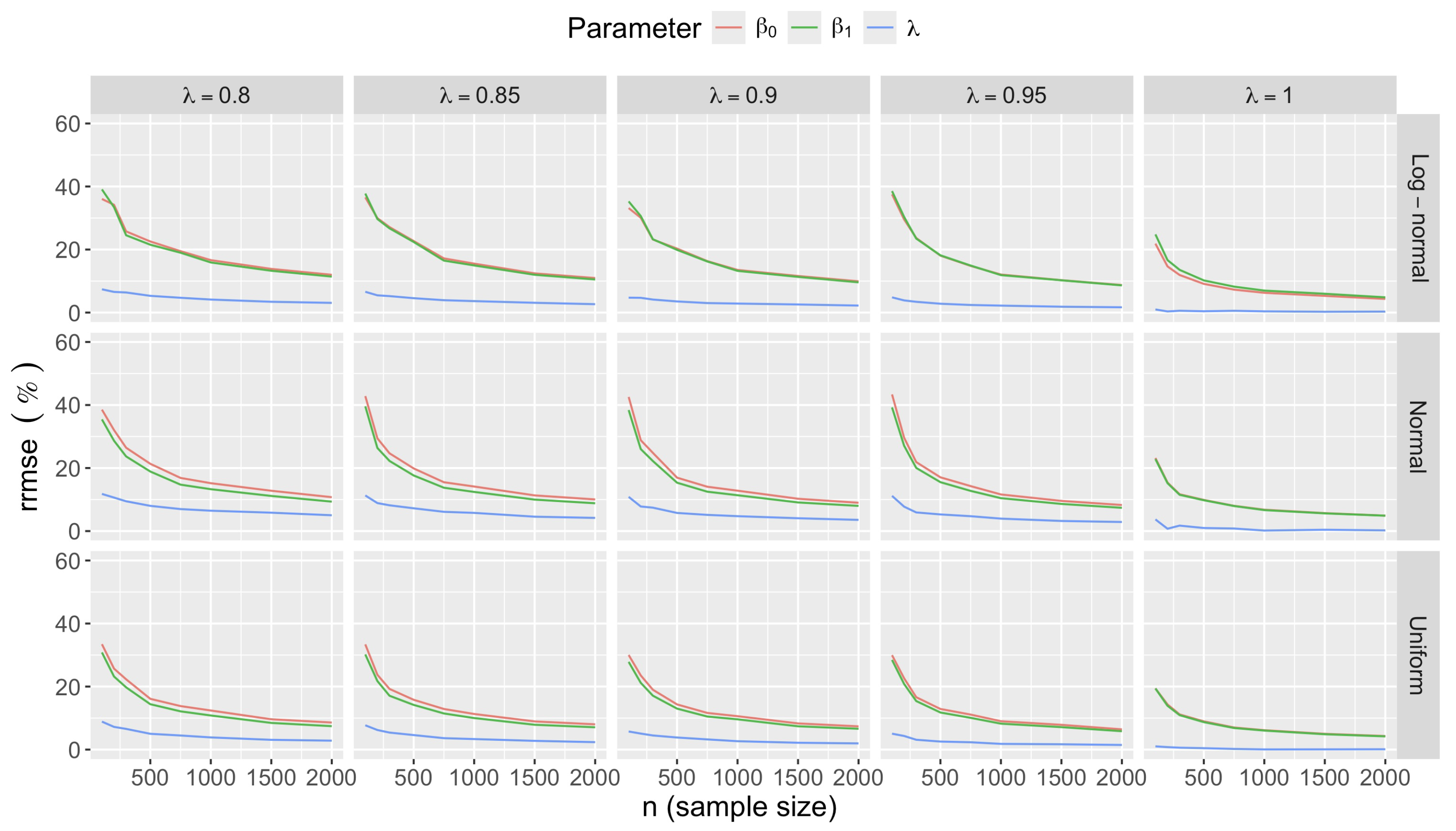
Figure A24.
Relative root mean square error () of Penalized Maximum Likelihood estimates of multistage binomial model parameters , and under the MSB model data generation process in Equation (A22) with , , and .
Figure A24.
Relative root mean square error () of Penalized Maximum Likelihood estimates of multistage binomial model parameters , and under the MSB model data generation process in Equation (A22) with , , and .
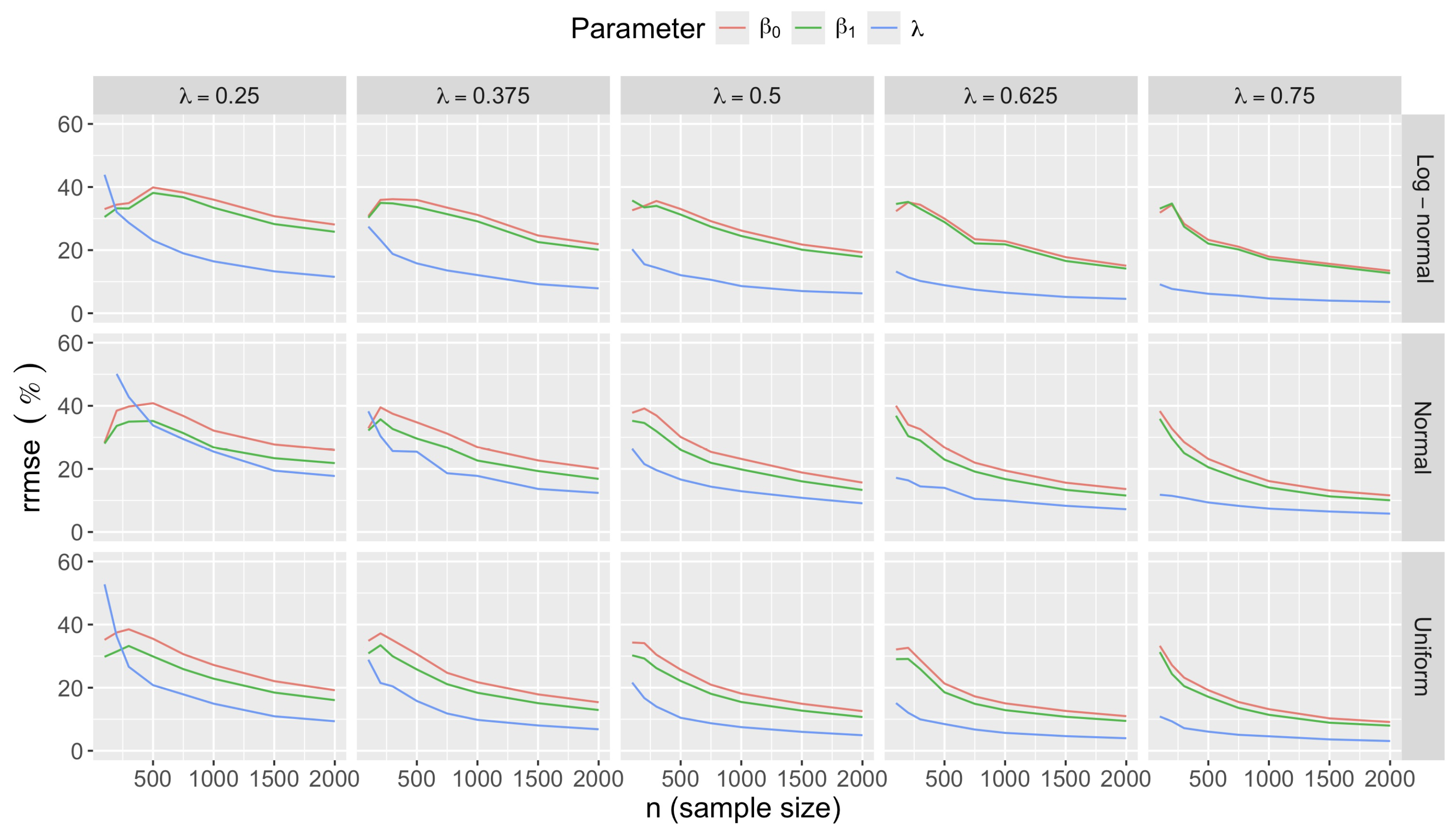
Figure A25.
Relative root mean square error (A22
) of Penalized Maximum Likelihood estimates of multistage binomial model parameters , and under the MSB model data generation process in Equation (A22) with , , and .
Figure A25.
Relative root mean square error (A22
) of Penalized Maximum Likelihood estimates of multistage binomial model parameters , and under the MSB model data generation process in Equation (A22) with , , and .
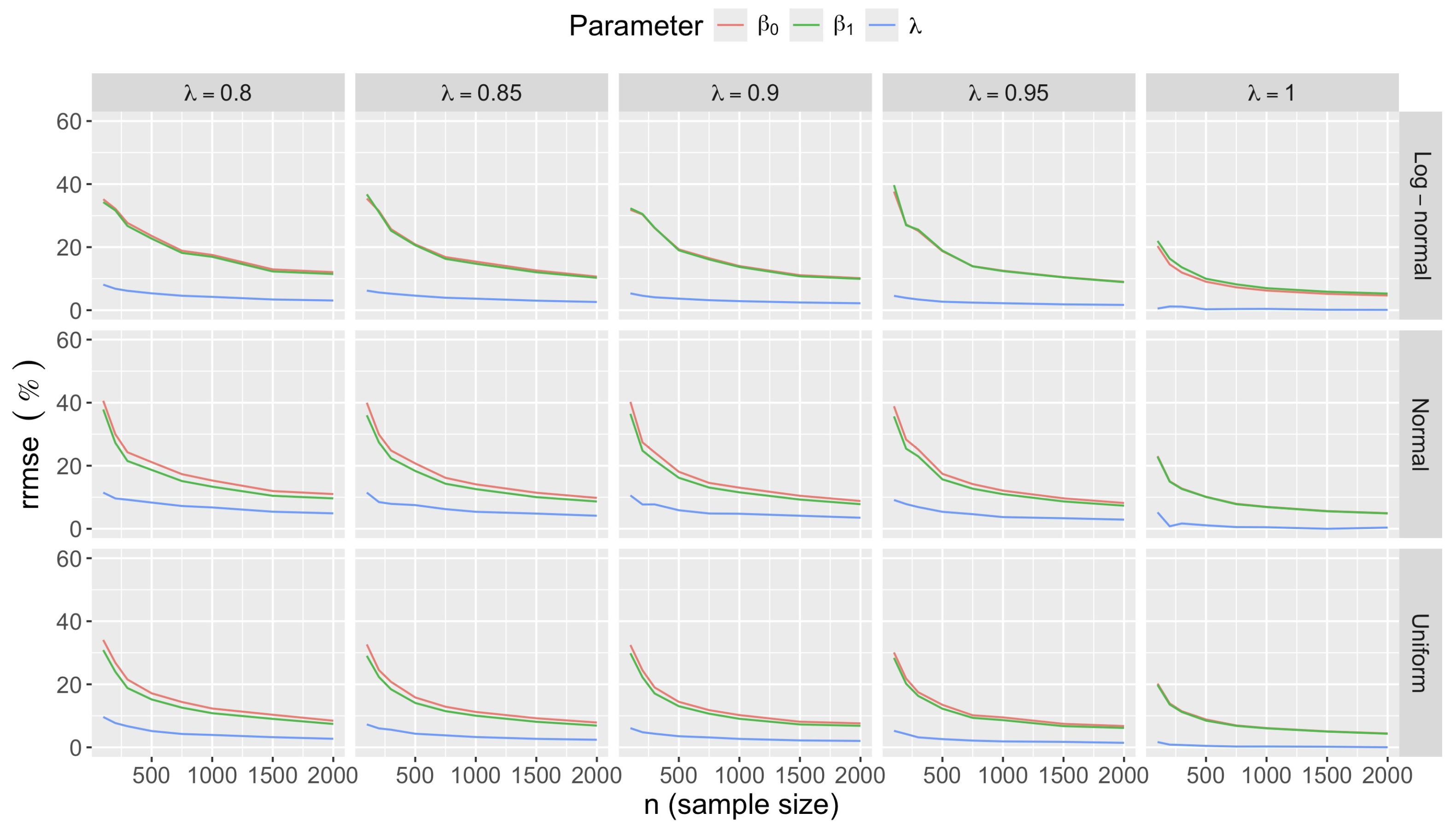
Figure A26.
Relative root mean square error () of Penalized Maximum Likelihood estimates of multistage binomial model parameters , and under the MSB model data generation process in Equation (A22) with , , and .
Figure A26.
Relative root mean square error () of Penalized Maximum Likelihood estimates of multistage binomial model parameters , and under the MSB model data generation process in Equation (A22) with , , and .
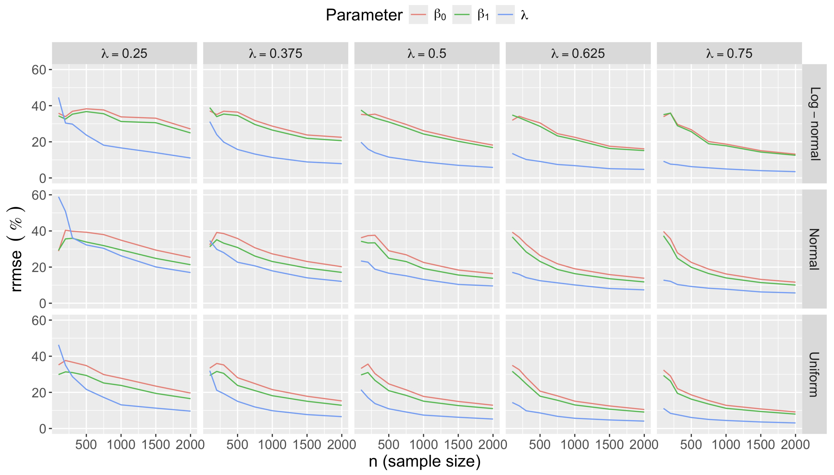
Figure A27.
Relative root mean square error () of Penalized Maximum Likelihood estimate of the slope under the MSB data generation process in Equation (A22) with (one predictor) for . The figure columns show the investigated pairs of true and values, and rows correspond to investigated distributions of predictor.
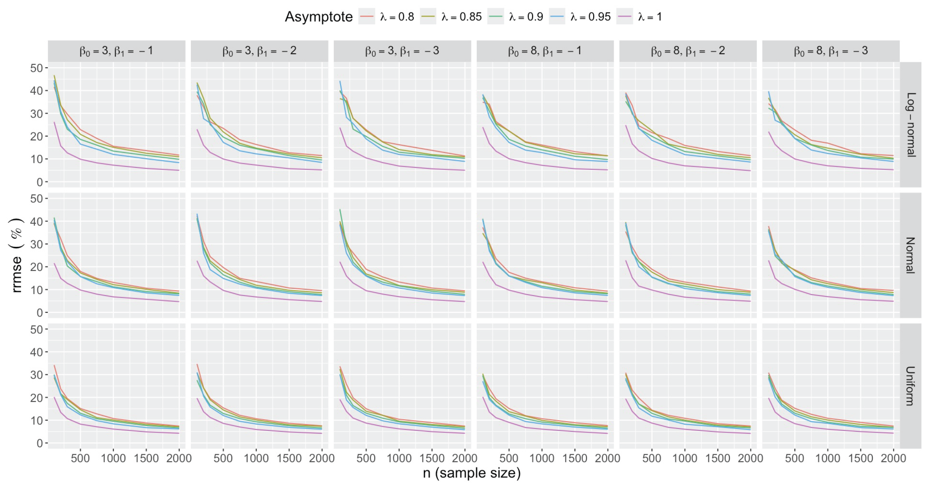
Figure A28.
Relative root mean square error () of Penalized Maximum Likelihood estimate of the slope under the MSB data generation process in Equation (A22) with (one predictor) for . The figure columns show the investigated pairs of true and values, and rows correspond to investigated distributions of predictor.
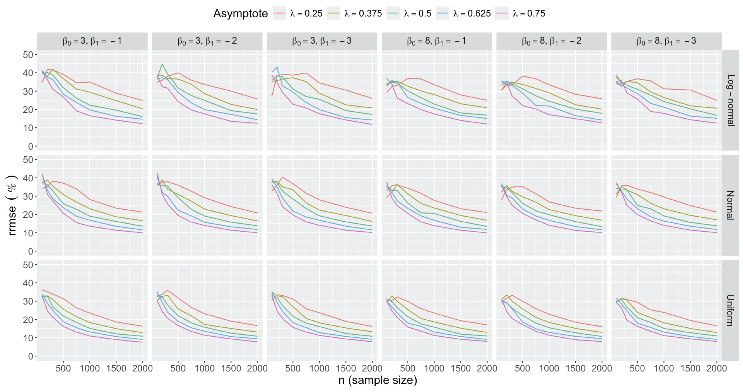
Appendix C.2.3. Sample Size Determination
In complement to Figure 4, Figure A29 and Figure A30 present the sample size n required to achieve a specified relative root mean square error for the PML estimate of the regression slope under the MSB data generation process in Equation (A22) with , for normal and log-normal predictor distributions, respectively.
Figure A29.
Sample size n required to achieve a specified relative root mean square error for the Penalized Maximum Likelihood estimate of the regression slope under the MSB data generation process in Equation (A22) with a normal predictor distribution, , and selected values.
Figure A29.
Sample size n required to achieve a specified relative root mean square error for the Penalized Maximum Likelihood estimate of the regression slope under the MSB data generation process in Equation (A22) with a normal predictor distribution, , and selected values.
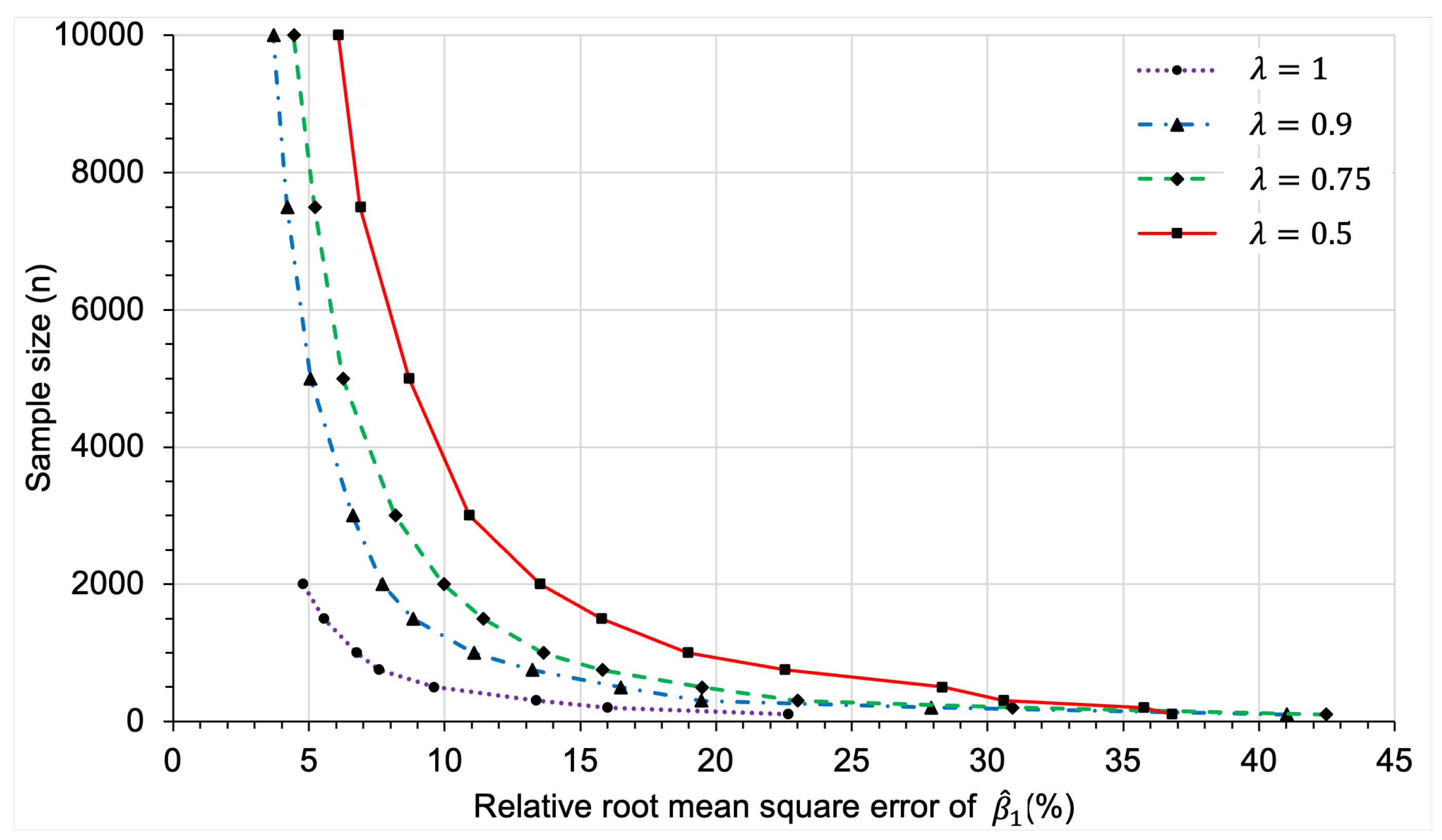
Figure A30.
Sample size n required to achieve a specified relative root mean square error for the Penalized Maximum Likelihood estimate of the regression slope under the MSB data generation process in Equation (A22) with a log-normal predictor distribution, , and selected values.
Figure A30.
Sample size n required to achieve a specified relative root mean square error for the Penalized Maximum Likelihood estimate of the regression slope under the MSB data generation process in Equation (A22) with a log-normal predictor distribution, , and selected values.
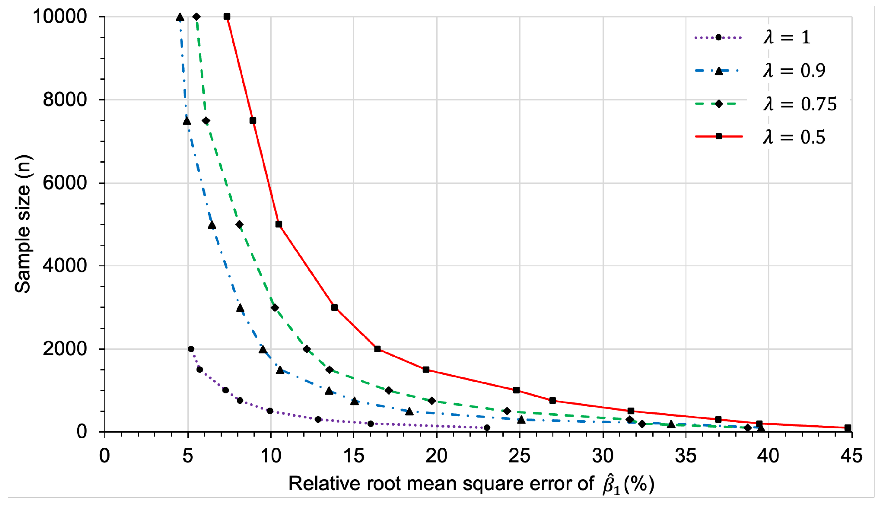
References
- Harris, J.K. Primer on binary logistic regression. Family medicine and community health 2021, 9, e001290. [CrossRef]
- Zabor, E.C.; Reddy, C.A.; Tendulkar, R.D.; Patil, S. Logistic regression in clinical studies. International Journal of Radiation Oncology* Biology* Physics 2022, 112, 271–277. [CrossRef]
- Halvorson, M.A.; McCabe, C.J.; Kim, D.S.; Cao, X.; King, K.M. Making sense of some odd ratios: A tutorial and improvements to present practices in reporting and visualizing quantities of interest for binary and count outcome models. Psychology of Addictive Behaviors 2022, 36, 284. [CrossRef]
- Nelder, J.A.; Wedderburn, R.W. Generalized linear models. Journal of the Royal Statistical Society: Series A (General) 1972, 135, 370–384.
- Webster, A.J. Multi-stage models for the failure of complex systems, cascading disasters, and the onset of disease. PloS one 2019, 14, e0216422. [CrossRef]
- Fröhlich, F.; Theis, F.J.; Rädler, J.O.; Hasenauer, J. Parameter estimation for dynamical systems with discrete events and logical operations. Bioinformatics 2017, 33, 1049–1056. [CrossRef]
- Zhang, T.; Rohlfs, R.; Schwartz, R. Implementation of a discrete event simulator for biological self-assembly systems. In Proceedings of the Proceedings of the Winter Simulation Conference, 2005. IEEE, 2005, pp. 9–pp.
- Manhart, M.; Morozov, A.V. Protein folding and binding can emerge as evolutionary spandrels through structural coupling. Proceedings of the National Academy of Sciences 2015, 112, 1797–1802. [CrossRef]
- Scarborough, P.; Nnoaham, K.E.; Clarke, D.; Capewell, S.; Rayner, M. Modelling the impact of a healthy diet on cardiovascular disease and cancer mortality. J Epidemiol Community Health 2012, 66, 420–426. [CrossRef]
- Walter, S.; Holford, T. Additive, multiplicative, and other models for disease risks. American Journal of Epidemiology 1978, 108, 341–346. [CrossRef]
- Zhang, X.; Fröhlich, H.; Grigoriev, D.; Vakulenko, S.; Zimmermann, J.; Weber, A.G. A simple 3-parameter model for cancer incidences. Scientific Reports 2018, 8, 3388. [CrossRef]
- Wu, S.; Powers, S.; Zhu, W.; Hannun, Y.A. Substantial contribution of extrinsic risk factors to cancer development. Nature 2016, 529, 43–47.
- Peto, R. Epidemiology, multistage models, and short-term mutagenicity tests. International Journal of Epidemiology 2016, 45, 621–637. [CrossRef]
- Wacholder, S.; Han, S.S.; Weinberg, C.R. Inference from a multiplicative model of joint genetic effects for ovarian cancer risk. Journal of the National Cancer Institute 2011, 103, 82–83. [CrossRef]
- Calabrese, P.; Shibata, D. A simple algebraic cancer equation: calculating how cancers may arise with normal mutation rates. BMC cancer 2010, 10, 1–12. [CrossRef]
- Siemiatycki, J.; Thomas, D.C. Biological models and statistical interactions: an example from multistage carcinogenesis. International journal of epidemiology 1981, 10, 383–387. [CrossRef]
- Armitage, P. Multistage models of carcinogenesis. Environmental health perspectives 1985, 63, 195–201.
- Loomba, R.; Yang, H.I.; Su, J.; Brenner, D.; Iloeje, U.; Chen, C.J. Obesity and alcohol synergize to increase the risk of incident hepatocellular carcinoma in men. Clinical Gastroenterology and Hepatology 2010, 8, 891–898. [CrossRef]
- Ishak, K.J.; Kreif, N.; Benedict, A.; Muszbek, N. Overview of parametric survival analysis for health-economic applications. Pharmacoeconomics 2013, 31, 663–675. [CrossRef]
- Chang, Y.T.; Wu, J.L.; Hsu, C.C.; Wang, J.D.; Sung, J.M. Diabetes and end-stage renal disease synergistically contribute to increased incidence of cardiovascular events: a nationwide follow-up study during 1998–2009. Diabetes care 2014, 37, 277–285. [CrossRef]
- Ramírez-Aldana, R.; Gomez-Verjan, J.C.; Bello-Chavolla, O.Y.; García-Peña, C. Spatial epidemiological study of the distribution, clustering, and risk factors associated with early COVID-19 mortality in Mexico. PloS one 2021, 16, e0254884. [CrossRef]
- Lee, A.; Mavaddat, N.; Wilcox, A.N.; Cunningham, A.P.; Carver, T.; Hartley, S.; Babb de Villiers, C.; Izquierdo, A.; Simard, J.; Schmidt, M.K.; et al. BOADICEA: a comprehensive breast cancer risk prediction model incorporating genetic and nongenetic risk factors. Genetics in Medicine 2019, 21, 1708–1718. [CrossRef]
- Di Angelantonio, E.; Kaptoge, S.; Wormser, D.; Willeit, P.; Butterworth, A.S.; Bansal, N.; O’Keeffe, L.M.; Gao, P.; Wood, A.M.; Burgess, S.; et al. Association of cardiometabolic multimorbidity with mortality. Jama 2015, 314, 52–60.
- Ott, J.; Ullrich, A.; Mascarenhas, M.; Stevens, G. Global cancer incidence and mortality caused by behavior and infection. Journal of public health 2011, 33, 223–233. [CrossRef]
- Lee, P. Relation between exposure to asbestos and smoking jointly and the risk of lung cancer. Occupational and environmental medicine 2001, 58, 145–153. [CrossRef]
- Katz, K.A. The (relative) risks of using odds ratios. Archives of dermatology 2006, 142, 761–764. [CrossRef]
- Greenland, S. Noncollapsibility, confounding, and sparse-data bias. Part 1: The oddities of odds. Journal of clinical epidemiology 2021, 138, 178–181. [CrossRef]
- Greenland, S. Noncollapsibility, confounding, and sparse-data bias. Part 2: What should researchers make of persistent controversies about the odds ratio? Journal of clinical epidemiology 2021, 139, 264–268. [CrossRef]
- Burgess, S. Estimating and contextualizing the attenuation of odds ratios due to non collapsibility. Communications in Statistics-Theory and Methods 2017, 46, 786–804. [CrossRef]
- Janani, L.; Mansournia, M.A.; Nourijeylani, K.; Mahmoodi, M.; Mohammad, K. Statistical issues in estimation of adjusted risk ratio in prospective studies. Archives of Iranian medicine 2015, 18, 0–0.
- Correia, K.; Williams, P.L. Estimating the relative excess risk due to interaction in clustered-data settings. American Journal of Epidemiology 2018, 187, 2470–2480. [CrossRef]
- Marschner, I.C. Relative risk regression for binary outcomes: methods and recommendations. Australian & New Zealand Journal of Statistics 2015, 57, 437–462. [CrossRef]
- Dwivedi, A.K.; Mallawaarachchi, I.; Lee, S.; Tarwater, P. Methods for estimating relative risk in studies of common binary outcomes. Journal of applied statistics 2014, 41, 484–500. [CrossRef]
- Chu, H.; Nie, L.; Chen, Y.; Huang, Y.; Sun, W. Bivariate random effects models for meta-analysis of comparative studies with binary outcomes: methods for the absolute risk difference and relative risk. Statistical methods in medical research 2012, 21, 621–633. [CrossRef]
- Hall, D.B. Zero-inflated Poisson and binomial regression with random effects: a case study. Biometrics 2000, 56, 1030–1039. [CrossRef]
- Richardson, T.S.; Robins, J.M.; Wang, L. On modeling and estimation for the relative risk and risk difference. Journal of the American Statistical Association 2017, 112, 1121–1130. [CrossRef]
- Yin, J.; Markes, S.; Richardson, T.S.; Wang, L. Multiplicative effect modelling: the general case. Biometrika 2022, 109, 559–566. [CrossRef]
- Doi, S.A.; Furuya-Kanamori, L.; Xu, C.; Lin, L.; Chivese, T.; Thalib, L. Controversy and debate: questionable utility of the relative risk in clinical research: paper 1: a call for change to practice. Journal of clinical epidemiology 2022, 142, 271–279. [CrossRef]
- Xiao, M.; Chen, Y.; Cole, S.R.; MacLehose, R.F.; Richardson, D.B.; Chu, H. Controversy and Debate: Questionable utility of the relative risk in clinical research: Paper 2: Is the Odds Ratio “portable” in meta-analysis? Time to consider bivariate generalized linear mixed model. Journal of Clinical Epidemiology 2022, 142, 280–287. [CrossRef]
- Xiao, M.; Chu, H.; Cole, S.R.; Chen, Y.; MacLehose, R.F.; Richardson, D.B.; Greenland, S. Controversy and Debate: Questionable utility of the relative risk in clinical research: Paper 4: Odds Ratios are far from “portable”—A call to use realistic models for effect variation in meta-analysis. Journal of Clinical Epidemiology 2022, 142, 294–304. [CrossRef]
- Suhail A, D.; Furuya-Kanamori, L.; Xu, C.; Lin, L.; Chivese, T.; Thalib, L. Questionable utility of the relative risk in clinical research: A call for change to practice. J Clin Epidemiol 2020.
- Mood, C. Logistic regression: Uncovering unobserved heterogeneity, 2017. 341160.
- Mood, C. Logistic regression: Why we cannot do what we think we can do, and what we can do about it. European sociological review 2010, 26, 67–82. [CrossRef]
- Cramer, J.S. Omitted variables and misspecified disturbances in the logit model. Technical report, Tinbergen Institute Discussion Paper, 2005.
- Yatchew, A.; Griliches, Z. Specification error in probit models. The Review of Economics and Statistics 1985, pp. 134–139. [CrossRef]
- Lee, L.F. Specification error in multinomial logit models: Analysis of the omitted variable bias. Journal of Econometrics 1982, 20, 197–209.
- Buis, M.L. Logistic regression: When can we do what we think we can do, 2017.
- Brzoska, P.; Sauzet, O.; Breckenkamp, J. Unobserved heterogeneity and the comparison of coefficients across nested logistic regression models: how to avoid comparing apples and oranges. International Journal of Public Health 2017, 62, 517–520. [CrossRef]
- Cologne, J.; Furukawa, K.; Grant, E.J.; Abbott, R.D. Effects of omitting non-confounding predictors from general relative-risk models for binary outcomes. Journal of Epidemiology 2019, 29, 116–122. [CrossRef]
- Schuster, N.A.; Twisk, J.W.; Ter Riet, G.; Heymans, M.W.; Rijnhart, J.J. Noncollapsibility and its role in quantifying confounding bias in logistic regression. BMC medical research methodology 2021, 21, 1–9. [CrossRef]
- Berkson, J. Are there two regressions? Journal of the american statistical association 1950, 45, 164–180.
- King, G.; Zeng, L. Logistic regression in rare events data. Political analysis 2001, 9, 137–163. [CrossRef]
- Huang, F.L. Alternatives to logistic regression models in experimental studies. The Journal of Experimental Education 2022, 90, 213–228. [CrossRef]
- Greenland, S.; Mansournia, M.A. Penalization, bias reduction, and default priors in logistic and related categorical and survival regressions. Statistics in medicine 2015, 34, 3133–3143. [CrossRef]
- Firth, D. Bias reduction of maximum likelihood estimates. Biometrika 1993, 80, 27–38.
- Albert, A.; Anderson, J.A. On the existence of maximum likelihood estimates in logistic regression models. Biometrika 1984, 71, 1–10.
- Heinze, G.; Schemper, M. A solution to the problem of separation in logistic regression. Statistics in medicine 2002, 21, 2409–2419. [CrossRef]
- Zeng, G.; Zeng, E. On the relationship between multicollinearity and separation in logistic regression. Communications in Statistics-Simulation and Computation 2021, 50, 1989–1997. [CrossRef]
- Mansournia, M.A.; Geroldinger, A.; Greenland, S.; Heinze, G. Separation in logistic regression: causes, consequences, and control. American journal of epidemiology 2018, 187, 864–870. [CrossRef]
- Rainey, C. Dealing with separation in logistic regression models. Political Analysis 2016, 24, 339–355. [CrossRef]
- Botes, M.; Fletcher, L. Comparing logistic regression methods for a sparse data set when complete separation is present. In Proceedings of the Annual Proceedings of the South African Statistical Association Conference. South African Statistical Association (SASA), 2014, number con-1 in 2014, pp. 1–8.
- Hauck Jr, W.W.; Donner, A. Wald’s test as applied to hypotheses in logit analysis. Journal of the american statistical association 1977, 72, 851–853.
- Diop, A.; Diop, A.; Dupuy, J.F. Maximum likelihood estimation in the logistic regression model with a cure fraction. Electronic Journal of Statistics 2011, 5, 460–483.
- Diop, A.; Diop, A.; Dupuy, J.F. Simulation-based inference in a zero-inflated Bernoulli regression model. Communications in Statistics-Simulation and Computation 2016, 45, 3597–3614.
- Diallo, A.O.; Diop, A.; Dupuy, J.F. Asymptotic properties of the maximum-likelihood estimator in zero-inflated binomial regression. Communications in Statistics-Theory and Methods 2017, 46, 9930–9948. [CrossRef]
- Pho, K.H. Goodness of fit test for a zero-inflated Bernoulli regression model. Communications in Statistics-Simulation and Computation 2024, 53, 756–771. [CrossRef]
- Diop, A.; Ba, D.B.; Lo, F. Asymptotic properties in the Probit-Zero-inflated Binomial regression model. arXiv preprint arXiv:2105.00483 2021.
- Garel, M.; Solberg, E.J.; Sæther, B.E.; Grøtan, V.; Tufto, J.; Heim, M. Age, size, and spatiotemporal variation in ovulation patterns of a seasonal breeder, the Norwegian moose (Alces alces). The American Naturalist 2009, 173, 89–104.
- Longford, N. Analysis of Covariance. In International Encyclopedia of Education (Third Edition), Third Edition ed.; Peterson, P.; Baker, E.; McGaw, B., Eds.; Elsevier: Oxford, 2010; pp. 18–24. [CrossRef]
- Pan, J.; Thompson, R. Gauss-Hermite quadrature approximation for estimation in generalised linear mixed models. Computational statistics 2003, 18, 57–78. [CrossRef]
- Rabe-Hesketh, S.; Skrondal, A.; Pickles, A. Reliable estimation of generalized linear mixed models using adaptive quadrature. The Stata Journal 2002, 2, 1–21. [CrossRef]
- Asheri, H.; Hosseini, R.; Araabi, B.N. A new EM algorithm for flexibly tied GMMs with large number of components. Pattern recognition 2021, 114, 107836. [CrossRef]
- Dempster, A.P.; Laird, N.M.; Rubin, D.B. Maximum likelihood from incomplete data via the EM algorithm. Journal of the royal statistical society: series B (methodological) 1977, 39, 1–22. [CrossRef]
- Wang, Z.; Louis, T.A. Matching conditional and marginal shapes in binary random intercept models using a bridge distribution function. Biometrika 2003, 90, 765–775. [CrossRef]
- Azzalini, A.; Valle, A.D. The multivariate skew-normal distribution. Biometrika 1996, 83, 715–726. [CrossRef]
- Ghosh, P. Corrected Probability Mass Function of the Binomial Distribution. Resonance 2021, 26, 1721–1724.
- Shklyar, S. Identifiability of logistic regression with homoscedastic error: Berkson model. Modern Stochastics: Theory and Applications 2015, 2, 131–146. [CrossRef]
- Küchenhoff, H. The identification of logistic regression models with errors in the variables. Statistical Papers 1995, 36, 41–47. [CrossRef]
- Al-Shaaibi, M.; Wesonga, R. Bias reduction in the logistic model parameters with the LogF (1, 1) penalty under MAR assumption. Frontiers in Applied Mathematics and Statistics 2022, 8, 1052752. [CrossRef]
- Heinze, G.; Puhr, R. Bias-reduced and separation-proof conditional logistic regression with small or sparse data sets. Statistics in medicine 2010, 29, 770–777. [CrossRef]
- Heinze, G.; Ploner, M. Fixing the nonconvergence bug in logistic regression with SPLUS and SAS. Computer methods and programs in biomedicine 2003, 71, 181–187. [CrossRef]
- Jeffreys, H. The theory of probability; OuP Oxford, 1998.
- Fisher, R.A. On the mathematical foundations of theoretical statistics. Philosophical transactions of the Royal Society of London. Series A, containing papers of a mathematical or physical character 1922, 222, 309–368.
- R Core Team. R: A Language and Environment for Statistical Computing. R Foundation for Statistical Computing, Vienna, Austria, 2025.
- Susko, E. Likelihood ratio tests with boundary constraints using data-dependent degrees of freedom. Biometrika 2013, 100, 1019–1023. [CrossRef]
- Shapiro, A. Asymptotic distribution of test statistics in the analysis of moment structures under inequality constraints. Biometrika 1985, 72, 133–144.
- Molenberghs, G.; Verbeke, G. Likelihood ratio, score, and Wald tests in a constrained parameter space. The American Statistician 2007, 61, 22–27. [CrossRef]
- Mitchell, J.D.; Allman, E.S.; Rhodes, J.A. Hypothesis testing near singularities and boundaries. Electronic journal of statistics 2019, 13, 2150. [CrossRef]
- Baey, C.; Cournède, P.H.; Kuhn, E. Asymptotic distribution of likelihood ratio test statistics for variance components in nonlinear mixed effects models. Computational Statistics & Data Analysis 2019, 135, 107–122. [CrossRef]
- Xu, C.; Bull, S.B. Penalized maximum likelihood inference under the mixture cure model in sparse data. Statistics in Medicine 2023, 42, 2134–2161. [CrossRef]
- Drton, M.; Williams, B. Quantifying the failure of bootstrap likelihood ratio tests. Biometrika 2011, 98, 919–934. [CrossRef]
- Cameron, A.C.; Windmeijer, F.A. An R-squared measure of goodness of fit for some common nonlinear regression models. Journal of econometrics 1997, 77, 329–342. [CrossRef]
- Morris, T.P.; White, I.R.; Crowther, M.J. Using simulation studies to evaluate statistical methods. Statistics in Medicine 2019, 38, 2074–2102. [CrossRef]
- Cribari-Neto, F.; Zeileis, A. Beta Regression in R. Journal of Statistical Software 2010, 34, 1–24. [CrossRef]
- Gueorguieva, R. A multivariate generalized linear mixed model for joint modelling of clustered outcomes in the exponential family. Statistical modelling 2001, 1, 177–193.
- Bonat, W.H.; Jørgensen, B. Multivariate covariance generalized linear models. Journal of the Royal Statistical Society Series C: Applied Statistics 2016, 65, 649–675. [CrossRef]
- Kosmidis, I.; Firth, D. Bias reduction in exponential family nonlinear models. Biometrika 2009, 96, 793–804. [CrossRef]
- Kosmidis, I.; Firth, D. A generic algorithm for reducing bias in parametric estimation. Electronic Journal of Statistics 2010, 4, 1097–1112. [CrossRef]
- Blizzard, L.; Hosmer, W. Parameter estimation and goodness-of-fit in log binomial regression. Biometrical Journal 2006, 48, 5–22. [CrossRef]
- Bartlett, M.S. Properties of sufficiency and statistical tests. Proceedings of the royal society of london. series a-mathematical and physical sciences 1937, 160, 268–282. [CrossRef]
- Rao, C. Score test: historical review and recent developments. Advances in ranking and selection, multiple comparisons, and reliability: methodology and applications 2005, pp. 3–20.
- Tovissodé, C.F.; Diop, A.; Glèlè Kakaï, R. Inference in skew generalized t-link models for clustered binary outcome via a parameter-expanded EM algorithm. Plos one 2021, 16, e0249604. [CrossRef]
- Vrabel, R. A note on the matrix determinant lemma. International Journal of Pure and Applied Mathematics 2016, 111, 643–646.
- Guyon, X. Statistique et Econométrie : du modèle linéaire aux modèles non-linéaires; Ellipses, 2001; p. 205. ISBN 2-7298-0842-6.
- Efron, B.; Hinkley, D.V. Assessing the accuracy of the maximum likelihood estimator: Observed versus expected Fisher information. Biometrika 1978, 65, 457–483.
- Cao, X.; Spall, J.C. Relative performance of expected and observed Fisher information in covariance estimation for maximum likelihood estimates. In Proceedings of the 2012 American Control Conference (ACC). IEEE, 2012, pp. 1871–1876.
- Yuan, X.; Spall, J.C. Confidence intervals with expected and observed fisher information in the scalar case. In Proceedings of the 2020 American Control Conference (ACC). IEEE, 2020, pp. 2599–2604.
- Jiang, S.; Spall, J.C. Comparison between Expected and Observed Fisher Information in Interval Estimation. In Proceedings of the 2021 55th Annual Conference on Information Sciences and Systems (CISS). IEEE, 2021, pp. 1–6.
- Magnus, J.R.; Neudecker, H. Matrix differential calculus with applications to simple, Hadamard, and Kronecker products. Journal of Mathematical Psychology 1985, 29, 474–492. [CrossRef]
- Magnus, J.R.; Neudecker, H. The commutation matrix: some properties and applications. The annals of statistics 1979, 7, 381–394. [CrossRef]
- Hamid, H.A.; Wah, Y.B.; Xie, X.J.; Rahman, H.A.A. Assessing the effects of different types of covariates for binary logistic regression. In Proceedings of the AIP Conference Proceedings. American Institute of Physics, 2015, Vol. 1643, pp. 425–430.
Figure 1.
Scatter plot of the simulated working data points (with jitters to improve readability) as a function of the predictor (), the true viability curve, and the fitted curves using the Standard Logistic Regression (SLR) and the Multistage Logistic Regression (MLR) models.
Figure 1.
Scatter plot of the simulated working data points (with jitters to improve readability) as a function of the predictor (), the true viability curve, and the fitted curves using the Standard Logistic Regression (SLR) and the Multistage Logistic Regression (MLR) models.
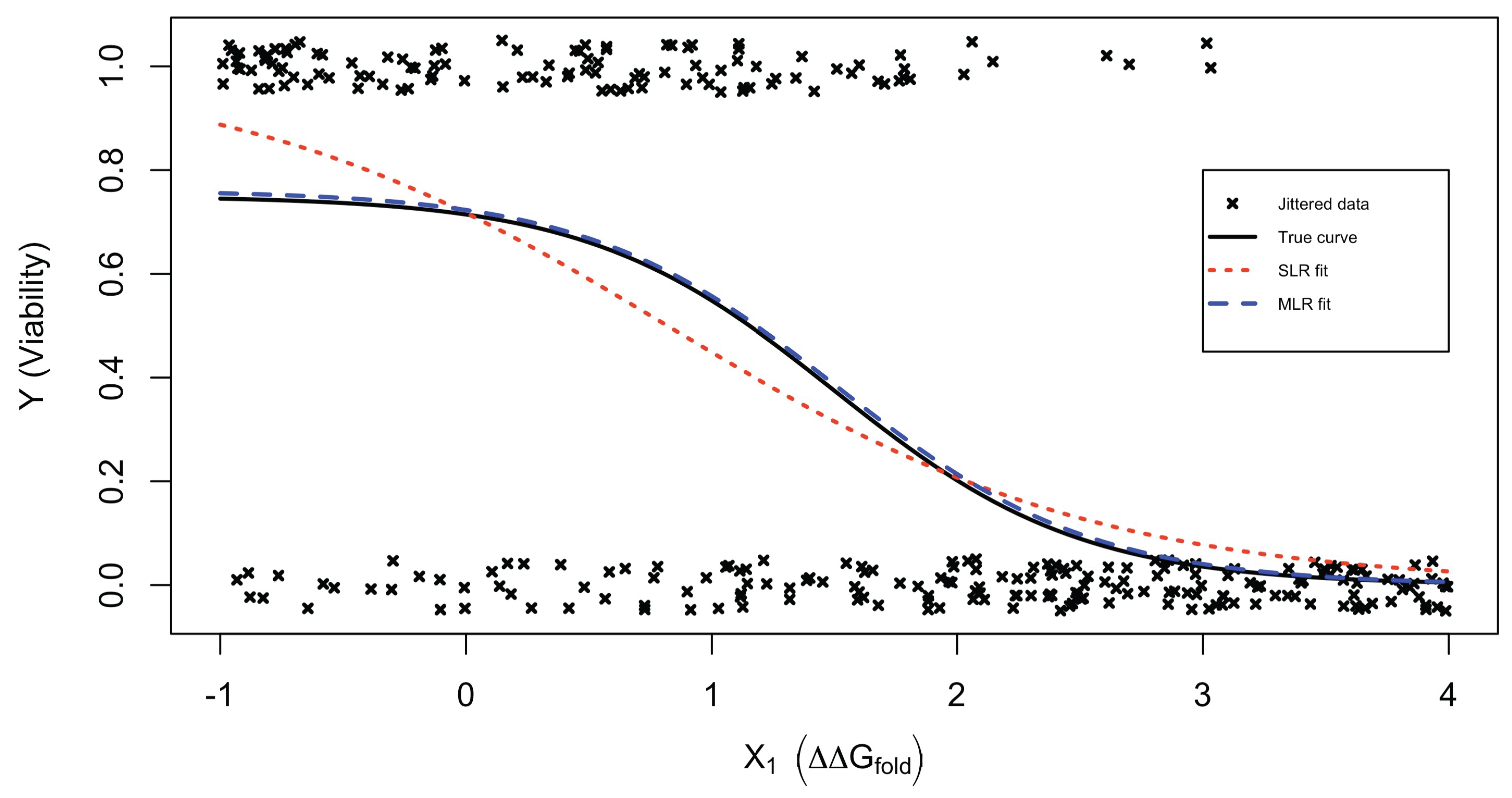
Figure 2.
Relative bias () of Penalized Maximum Likelihood estimates of multistage binomial model parameters , and under the MSB data generation process in Equation (17) with , . The figure columns show the investigated true values, and rows correspond to investigated distributions of predictor.
Figure 2.
Relative bias () of Penalized Maximum Likelihood estimates of multistage binomial model parameters , and under the MSB data generation process in Equation (17) with , . The figure columns show the investigated true values, and rows correspond to investigated distributions of predictor.
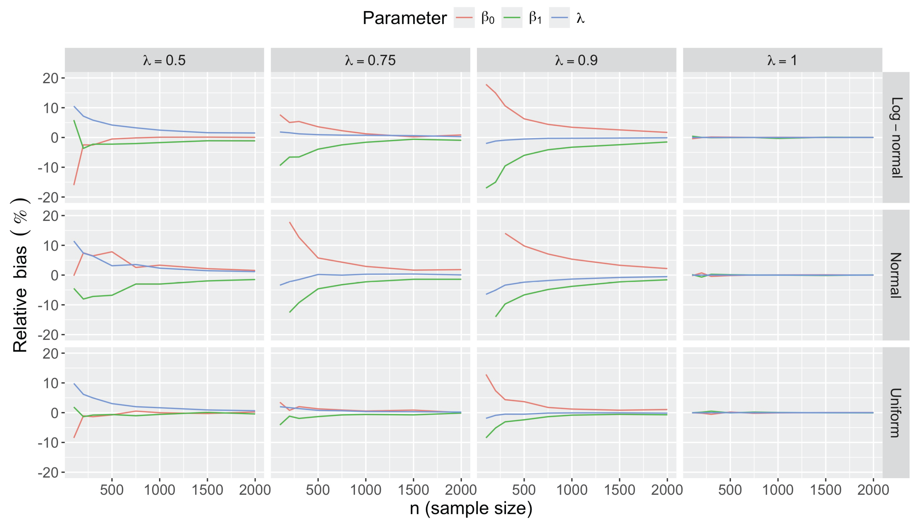
Figure 3.
Relative root mean square error () of Penalized Maximum Likelihood estimates of multistage binomial model parameters , and under the MSB data generation process in Equation (17) with , . The figure columns show the investigated true values, and rows correspond to investigated distributions of predictor.
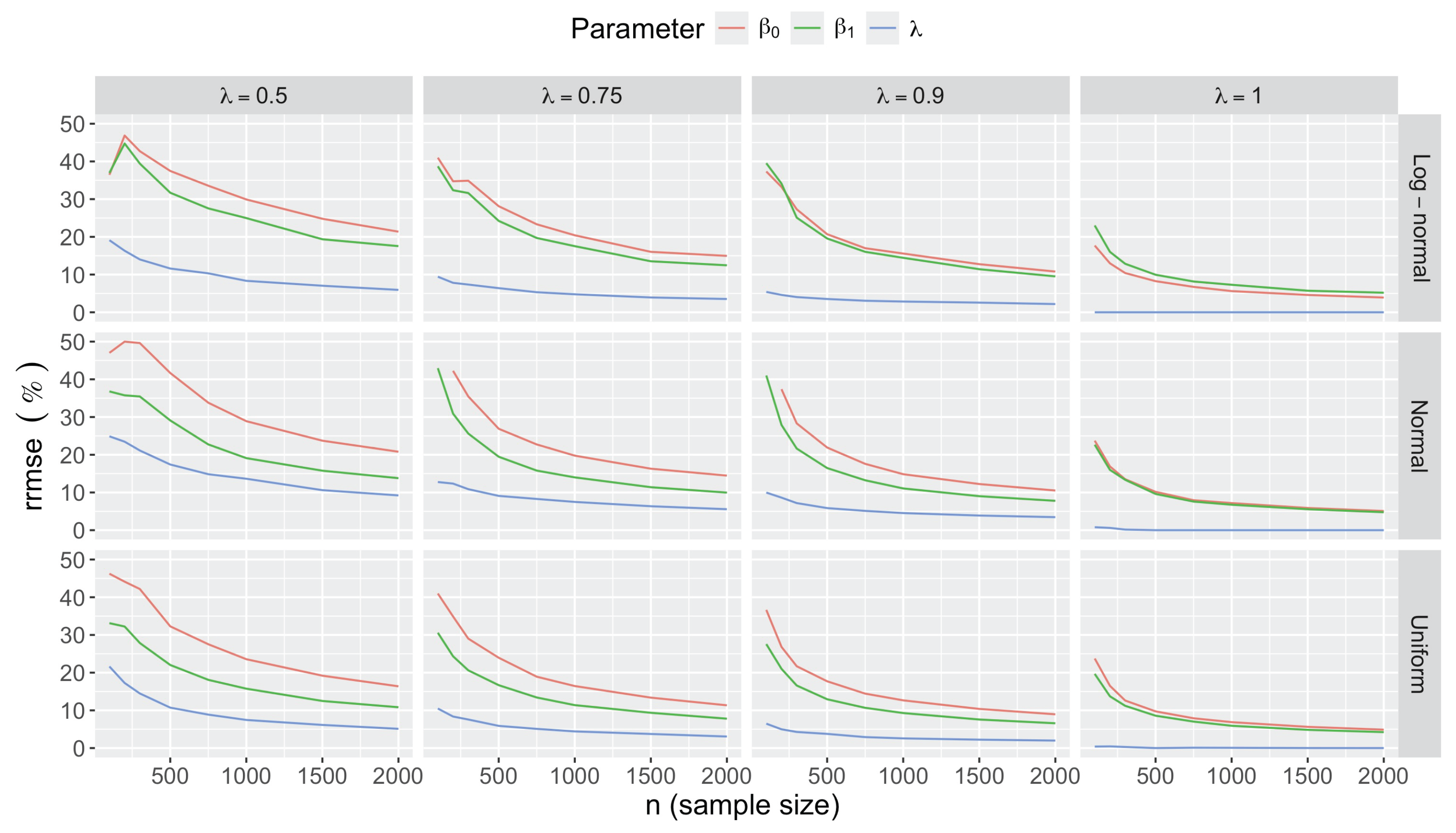
Figure 4.
Sample size n required to achieve a specified relative root mean square error for the Penalized Maximum Likelihood estimate of the regression slope under the MSB data generation process in Equation (17) with a uniform predictor distribution, , and selected values.
Figure 4.
Sample size n required to achieve a specified relative root mean square error for the Penalized Maximum Likelihood estimate of the regression slope under the MSB data generation process in Equation (17) with a uniform predictor distribution, , and selected values.
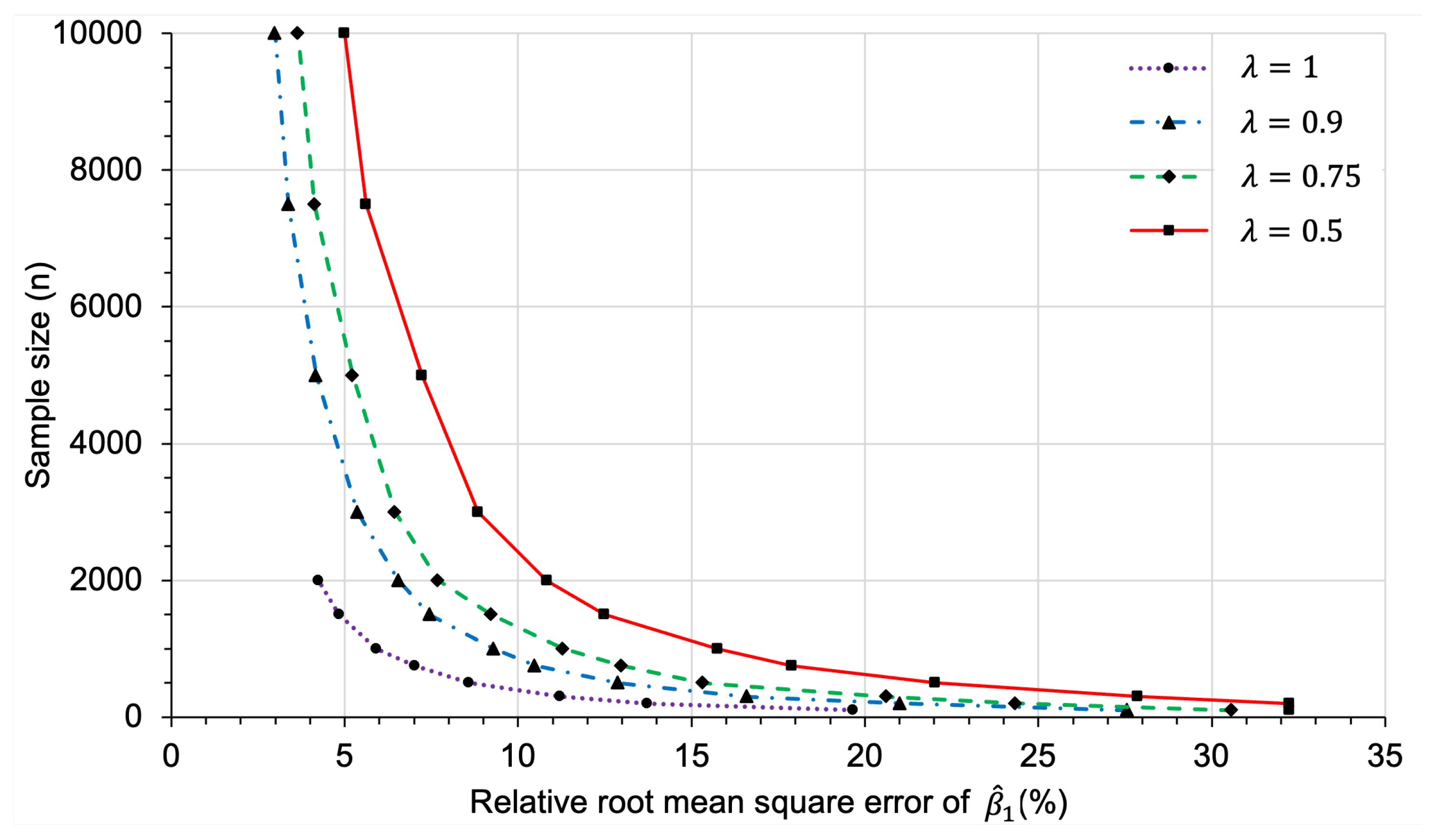
Figure 5.
Rejection rate of the Likelihood Ratio (LR) test of the null hypothesis () at the significance level of 5% under the MSB model data generation process in Equation (17) with , , and .
Figure 5.
Rejection rate of the Likelihood Ratio (LR) test of the null hypothesis () at the significance level of 5% under the MSB model data generation process in Equation (17) with , , and .
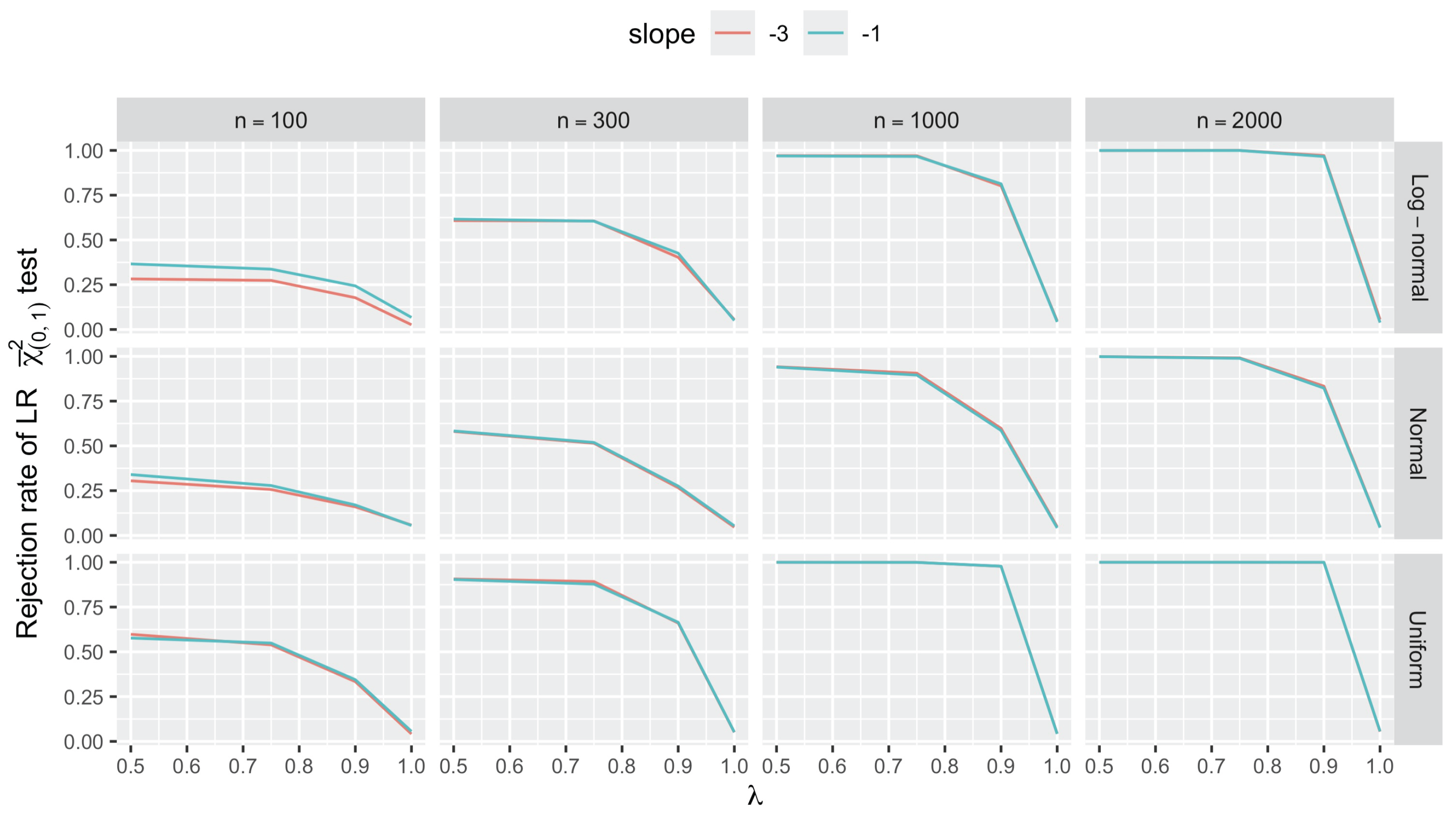
Figure 6.
Coverage probability of Penalized Maximum Likelihood estimates of multistage binomial model parameters (shown as beta[0]) and (shown as beta[1]) under the MSB data generation process in Equation (17) with , . The figure columns show the investigated true values, and rows correspond to investigated distributions of predictor.
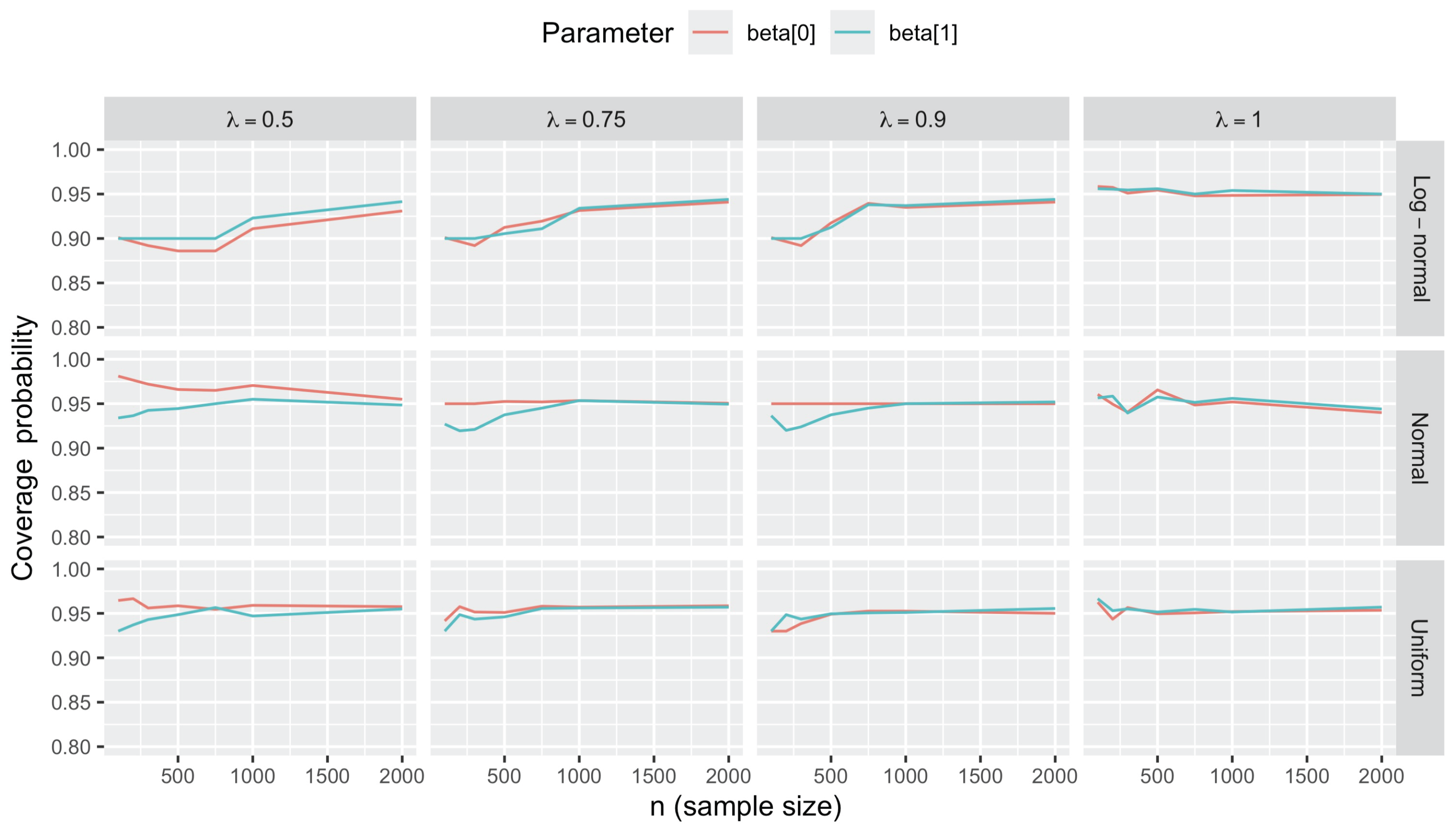
Figure 7.
Significance probability of Penalized Maximum Likelihood estimates of multistage binomial model parameters (shown as beta[0]) and (shown as beta[1]) under the MSB data generation process in Equation (17) with , . The figure columns show the investigated true values, and rows correspond to investigated distributions of predictor.
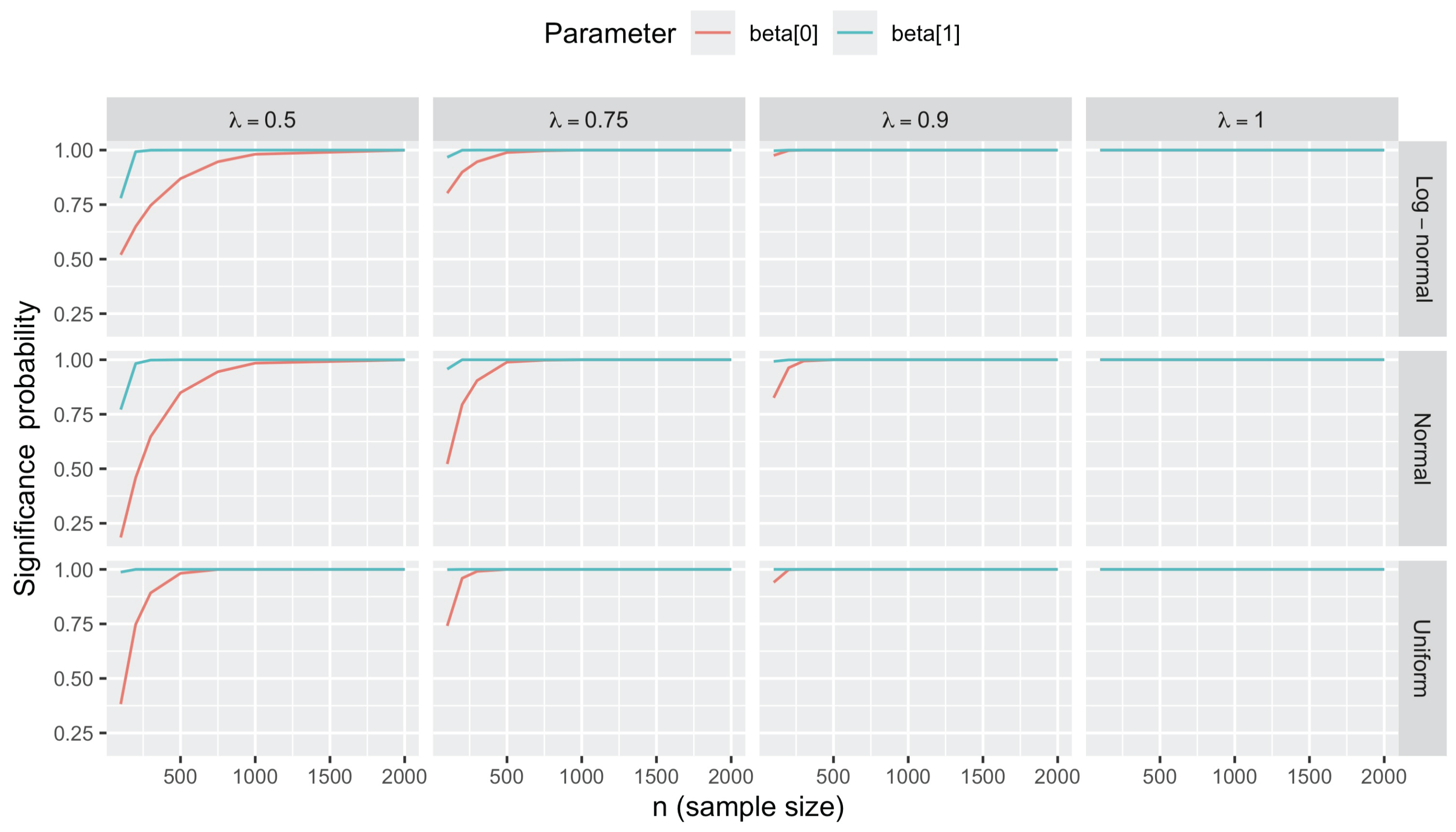
Table 1.
Simulated example 1 (): simple logistic regression analysis for protein viability against folding stability (): comparison of Standard Logistic Regression (SLR) and Multistage Logistic Regression (MLR) model fits.
Table 1.
Simulated example 1 (): simple logistic regression analysis for protein viability against folding stability (): comparison of Standard Logistic Regression (SLR) and Multistage Logistic Regression (MLR) model fits.
| Parameter | SLR | MLR | |||
|---|---|---|---|---|---|
| Estimate (SE) | Estimate (SE) | ||||
| 0.9300 (0.2031) | [ 0.5319, 1.3281] | 2.9461 (0.8613) | [ 1.2581, 4.6342] | ||
| () | -1.1359 (0.1302) | [-1.3911, -0.8806] | -1.9427 (0.3915) | [-2.7100, -1.1755] | |
| - | - | 1.1586 (0.3262) | [ 0.5192, 1.7979] | ||
| - | - | 0.7611 (0.0593) | [ 0.6269, 0.8579] | ||
| Deviance | 277.4280 | 270.3012 | |||
| AIC | 281.4280 | 276.3012 | |||
| 0.3054 | 0.3232 | ||||
Table notes: SE are standard errors; refers to 95% confidence interval determined using the large sample normal approximation to the distribution of each estimate; (not a free model parameter) is computed from ; Deviance refers to the residual deviance of a model fit as compared to a null (constant) fit; is the percent deviance reduction achieved by including the predictor () in the fit [92]. Likelihood ratio test for the additional asymptote parameter in the MLR fit: , .
Table 2.
Simulated example 2 (): bivariate logistic regression analysis for protein viability against folding stability () and binding stability (): comparison of Zero-Inflated Logistic (ZIL) and Multistage Logistic Regression (MLR) model fits.
Table 2.
Simulated example 2 (): bivariate logistic regression analysis for protein viability against folding stability () and binding stability (): comparison of Zero-Inflated Logistic (ZIL) and Multistage Logistic Regression (MLR) model fits.
| Parameter | ZIL | MLR | |||
|---|---|---|---|---|---|
| Estimate (SE) | Estimate (SE) | ||||
| 1.2107 (0.3296) | [ 0.5648, 1.8566] | 2.9969 (1.1077) | [ 0.8259, 5.1679] | ||
| () | -1.1456 (0.1758) | [-1.4901, -0.8010] | -1.9110 (0.5003) | [-2.8916, -0.9304] | |
| 4.2708 (1.4974) | [ 1.3360, 7.2055] | 4.5245 (1.5648) | [ 1.4575, 7.5914] | ||
| () | -1.1949 (0.3353) | [-1.8520, -0.5378] | -1.2602 (0.3542) | [-1.9545, -0.5659] | |
| - | - | 1.5059 (0.4904) | [ 0.5447, 2.4671] | ||
| - | - | 0.8185 (0.0729) | [ 0.6329, 0.9218] | ||
| Deviance | 229.5335 | 222.5019 | |||
| AIC | 237.5335 | 232.5019 | |||
| 0.3678 | 0.3872 | ||||
Table notes: SE are standard errors; refers to 95% confidence interval determined using the large sample normal approximation to the distribution of each estimate; (not a free model parameter) is computed from ; Deviance refers to the residual deviance of a model fit as compared to a null (constant) fit; is the percent deviance reduction achieved by including the predictors () and () in the fit [92]. Likelihood ratio test for the additional asymptote parameter in the MLR fit: , .
Table 3.
Example 2: comparison of performance measures (mean estimates, relative biases and root mean square errors) for ZIL and MLR model fits using 2000 replicates of MLR data ().
Table 3.
Example 2: comparison of performance measures (mean estimates, relative biases and root mean square errors) for ZIL and MLR model fits using 2000 replicates of MLR data ().
| Measure | Model | Model parameter (true value) | Predictive power | ||||||
| (3) | (-2) | (3) | (-1) | (0.8) | |||||
| Mean | ZIL | 2.1830 | -1.6863 | 2.2972 | -0.8708 | - | 0.0333 | 0.9690 | |
| MLR | 3.3368 | -2.1564 | 3.2767 | -1.0685 | 0.8022 | 0.0280 | 0.9806 | ||
| (%) | ZIL | -27.23 | 15.69 | -23.43 | 12.92 | - | - | - | |
| MLR | 11.23 | -7.82 | 9.22 | -6.85 | 0.28 | - | - | ||
| (%) | ZIL | 50.42 | 34.49 | 45.00 | 30.40 | - | - | - | |
| MLR | 43.18 | 32.54 | 40.01 | 29.35 | 9.55 | - | - | ||
Table notes: The ZIL and MLR models differ by the presence of the additional parameter in the MLR model. The ZIL model assumes that . (mean absolute deviation) is the sample average of the absolute deviations between the predicted success probabilities () from a fit and the true success probabilities (). is the squared Pearson correlation coefficient between and .
Table 4.
Beta regression model fit to the relative root mean square error () of the estimate of the slope in a simple logistic regression with a multiplicative intercept .
Table 4.
Beta regression model fit to the relative root mean square error () of the estimate of the slope in a simple logistic regression with a multiplicative intercept .
| Term | Mean (log link) | Precision parameter (log link) | |||
| Estimate (SE) | Estimate (SE) | ||||
| Intercept | -0.8591 (0.0174) | [-0.8931, -0.8251] | 6.1178 (0.2054) | [ 5.7152, 6.5204] | |
| n | -0.0003 (0.0000) | [-0.0003, -0.0003] | 0.0020 (0.0002) | [ 0.0016, 0.0024] | |
| -0.6482 (0.0278) | [-0.7027, -0.5937] | -2.3751 (0.2475) | [-2.8602, -1.8899] | ||
| -0.0688 (0.0104) | [-0.0892, -0.0484] | 0.2182 (0.0741) | [ 0.0730, 0.3633] | ||
| -0.0026 (0.0027) | [-0.0078, 0.0026] | - | - | ||
| = Normal | 0.0942 (0.0190) | [ 0.0570, 0.1314] | -0.7010 (0.1460) | [-0.9872, -0.4149] | |
| = Log-normal | 0.1588 (0.0190) | [ 0.1216, 0.1960] | -0.6797 (0.1460) | [-0.9658, -0.3935] | |
| -0.0006 (0.0000) | [-0.0006, -0.0005] | -0.0012 (0.0002) | [-0.0016, -0.0007] | ||
| 0.0001 (0.0000) | [ 0.0001, 0.0001] | - | - | ||
| Normal) | 0.0001 (0.0001) | [ 0.0001, 0.0001] | 0.0006 (0.0001) | [ 0.0003, 0.0009] | |
| Log-normal) | 0.0001 (0.0001) | [ 0.0001, 0.0002] | 0.0003 (0.0001) | [ 0.0001, 0.0006] | |
| Normal) | 0.0499 (0.0293) | [-0.0075, 0.1072] | - | - | |
| Log-normal) | 0.1010 (0.0295) | [ 0.0432, 0.1588] | - | - | |
Table notes: the predictors include the sample size (), the asymptote parameter (), the intercept () and the slope () in the data model for simulations. The dependent variable in this beta regression fit is where is the relative root mean square error of expressed in percent of the true value (so ). The values were computed from 2000 Monte Carlo replicates of each simulation setting. The precision parameter is such that, if the mean of is denoted , the variance of is . The beta regression model was fitted using the R package betareg [94]. The model was initially fitted using all predictors and all two-order interactions as terms in the linear predictors of both and . Then, a backward selection was used to recursively drop the least important term based on Akaike’s Information Criterion (), but main terms (predictors) were not dropped from the linear predictors of the mean . SE denotes standard errors; refers to 95% confidence interval determined using the large sample normal approximation to the distribution of each estimate; , (squared correlation between linear predictor and link-transformed response).
Disclaimer/Publisher’s Note: The statements, opinions and data contained in all publications are solely those of the individual author(s) and contributor(s) and not of MDPI and/or the editor(s). MDPI and/or the editor(s) disclaim responsibility for any injury to people or property resulting from any ideas, methods, instructions or products referred to in the content. |
© 2025 by the authors. Licensee MDPI, Basel, Switzerland. This article is an open access article distributed under the terms and conditions of the Creative Commons Attribution (CC BY) license (http://creativecommons.org/licenses/by/4.0/).
Copyright: This open access article is published under a Creative Commons CC BY 4.0 license, which permit the free download, distribution, and reuse, provided that the author and preprint are cited in any reuse.


