
Submitted:
26 September 2025
Posted:
28 September 2025
You are already at the latest version
Abstract
Within the present paper, a framework for Physics Informed Neural Networks (PINN) is formulated for the analysis of frame structures in two dimensions. The individual structural elements are represented by Euler-Bernoulli beams with additional axial stiffness. The transverse and axial displacements are approximated by individual neural networks and the differential equations are considered by minimizing a global loss function within the simultaneous training process. As a novelty, the boundary conditions at the supports of the structure and the coupling conditions at the element connections are considered in a joined loss function and specific weighting factors are defined and tuned within the training. Several examples have been investigated: first a simple beam structure with varying cross section properties and second with a concentrated discrete load in order to investigated the applicability of the PINNs for structural analysis. Two more sophisticated examples with several elements connected at rigid corners were analyzed, where the fulfillment of the consistency of the displacements and the equilibrium conditions of the internal forces is a crucial condition within the loss function of the network training. The results of the PINN framework are verified successfully with traditional finite element solutions for the presented examples. Nevertheless, the weighting of the individual loss function terms is the crucial point in the presented approach, which will be discussed in the paper.
Keywords:
beam theory
; physics informed neural networks
; boundary conditions
; equilibrium conditions
; frame structures
1. Introduction
In the recent years, machine learning (ML) gained huge popularity and found its way in almost every field, where big amounts of data are available and can serve as basis for training of neural networks (NN) to automatize and speed up a large span of different processes. In fields of science, they can be used as surrogates of high cost models to reduce computation time or to offer higher accuracy in representing complicated relations, compared to traditional models. However, a purely data-driven ML approach lacks accuracy in situations, where data is very scarce or noisy and fails to generalize outside of the domain covered by the training data. Furthermore, if the data is biased and does not represent the real physical behavior properly, the trained NN will also produce a biased output.
Physics informed ML has emerged as a promising alternative to compensate for these weaknesses. Here, physical laws and known relations can be considered for the network training. A prominent variant is the Physics Informed Neural Network (PINN), which was already used for solving a wide range of problems involving partial differential equations, when making its first appearance [1]. Ever since it was successfully applied in fluid mechanics, optics, electromagnetism, thermodynamics, biophysics, quantum physics and many more disciplines [2,3]. PINNs also established valuable contributions in the field of structural engineering, where extensive data is usually expensive or difficult to obtain. Implementing constitutive relations and force equilibrium equations, which are also the basis for the finite element method (FEM), into the NN loss function, they are able to represent displacements and stresses under given loading conditions. This was conducted for several scenarios for beams [4,5,6], plates [4,7,8,9,10] and shells [11]. Considered approaches also generalize well to full 3D structures [4,10]. Furthermore, problems of linear elasticity [4,6] as well as elastoplasticity [12,13,14] and fracture [15,16] were successfully implemented.
Several improvements were developed since its introduction to make PINNs more flexible and efficient. While the original version works with the strong form of the PDE, alternative approaches were proposed, which aim to minimize an equivalent energy expression in the loss function [15,17]. This can improve convergence, especially when the respective PDE contains higher order derivatives. Transfer learning can speed up the training process significantly and enable PINNs to be applied to e.g. multiple different loading scenarios without completely retraining the model [10,12,15]. Loading conditions can also be included as an additional network input [7]. To apply PINNs to complex geometries or discontinuous materials more effectively, they can be divided into separate domains treated with individual coupled networks, as proposed in the extended PINN (XPINN) method [18]. On the other hand parametric PINNs (P2INNs) offer the possibility to change PDE parameters without requiring a retraining of the model. Currently PINNs do not outperform FEM when its comes to solving single forward problems. They could however offer significant speed up for problems, which require a large number of PDE solutions like parametric studies [19]. Instead of replacing the method, cheap FEM solutions can also be incorporated into the NN training, to increase the speed of network training [20]. Some merits of PINNs are that they do not require any meshing or discretization, are robust when dealing with noisy data [7,10] and can be scaled up to arbitrary dimensions [21]. Furthermore, they can easily be applied to inverse problems, which allows identification of unknown material parameters, system parameters or acting forces [5,6,22] or of hidden damage [8,23,24]. Most of the listed studies are limited to single structural components and simple geometries. The formalism established with XPINNs demonstrates possible extensions to more complex and composed systems. Kapoor et al. [6] concluded, that computing the dynamic behavior of two coupled bending beams did not reduce accuracy compared to a single beam solution, hinting at possible generalization of PINN applications to more complex composed systems. In Meethal et al. [20] a PINN was applied to a bigger truss structure made of 23 members of two different kinds using the nodal loads as input values to compute the nodal displacements.
These works bring up the idea of using PINNs within a modular framework for the computation of structural frames as an alternative to FEM software. However, this poses several challenges, some of which are investigated in this work. Variable cross-sectional properties are common throughout civil engineering, when the material should be used as efficiently as possible. Oftentimes the height or thickness of beams follows the bending moment distribution along the span, increasing in regions of high moment and decreasing where the demand is lower to optimize material usage. Instead of a discretization with beam elements of constant cross sectional properties, PINNs actually allow treating the modified PDE involving spatial derivatives of e.g. material parameters and beam thickness. In Faroughi et al. [25] this was already explored for a non-prismatic cantilever beams subjected to a uniform load. Furthermore, concentrated loads present a significant challenge to the described PINN setup because they cause discontinuities in the load and shear forces. The neural network used to estimate the deflection is however only capable of representing smooth functions. For a concentrated force acting on a hemisphere Bastek and Kochmann [11] approximated the load distribution with a Gaussian kernel.
To the best of our knowledge, none of the previous works has addressed frame structures composed of rods, that are subjected to both axial as well as transverse loading, which requires coupling the PDEs for bending and axial displacements. This study addresses this gap through a set of representative example structures. The remaining article is structured as follows. In Section 2 the governing PDEs for bending and axial displacements are displayed and the respective PINN implementation is described. Section 3 summarizes the results starting with the treatment of a cantilever beam with varying bending stiffness in Section 3.1, followed by investigation of the accuracy of the method for a concentrated load on a supported beam in Section 3.2. Finally the PINN is applied to two different frame structures each composed of three coupled elements to illustrate how the method handles the simultaneous treatment of axial and bending displacements and the coupling conditions at shared nodes, where multiple elements are connected. Section 4 summarizes and discusses the findings of this work.
2. Materials and Methods
2.1. Governing Equations for Beam Deflection and Axial Displacement
In order to solve the task of approximating beam deflections through a physical informed neural network (PINN), it is necessary to implement the existing physical knowledge about the problem at hand. For problems considering bending beams, the Euler-Bernoulli equation is considered. The differential equation describes the relationship between the beam displacement and the corresponding applied load [26]
The function describes the deflection of the one-dimensional beam in z direction under a distributed load . is the bending stiffness of the beam, which is often assumed to be constant. However, it can also be defined as a function over x, when E or I change over the beams length. In Figure 1 a simply supported beam is shown with the corresponding load and deflection function.
The derivatives of contain the information about the beam slope, denoted by and the governing internal forces, namely the bending moment, , and the shear force,
These equations contain the physical knowledge about the system to be analyzed and are considered within the loss function for the neural network training. In case of constant , the Euler-Bernoulli equation can be simplified as follows
Axial displacements are considered additionally to the bending deflection for each structural element. The differential equation for the corresponding tension bar is denoted as
where is the axial displacement, A is the cross section area and the term is the axial load function over the length. denotes the internal axial forces. Figure 2 shows a rod with the corresponding load and displacement functions.
For constant the differential equation simplifies to
In case of , the normal force in axial direction is constant and the first derivative of is sufficient to approximate the axial displacement
where F is a single axial force acting on the right side of the element as indicated in Figure 2.
2.2. Nondimensionalization
Data normalization is a common practice in traditional deep learning. It is a prerequisite processing step that involves scaling the input features of a dataset to obtain similar data magnitudes and ranges. However, this process is not generally applicable to physics problems, as the target solutions are typically not available and therefore it cannot be scaled. In the context of PINNs, it is imperative to ensure that the network outputs fall within a reasonable range. A common approach to ensure this is the nondimensionalization of the governing differential equation, a technique frequently employed in mathematics and physics [27]. Normalization and nondimensionalization are proven to enhance the training performance of neural networks by mitigating disparities in variable scales and improving convergence [6,28]. Nondimensionalization addresses problems with unstable network training due to differently scaled variables and is an effective method for enhancing training performance. The nondimensionalization of a differential equation involves the removal of all units from the equation and the uniform scaling of the variables.
First a constant bending stiffness of the beam is assumed. The Euler-Bernoulli equation’s independent variable is x and the two dependent variables are w and q. The physical parameters that are relevant to the problem are the length of the beam, denoted by L, and the bending stiffness . These parameters are selected as the characteristic scales. The dimensionless variables are defined as follows
The beam length, the beam slope, the bending moment and the shear force are not involved in nondimensionalizing the equation, but will be calculated as nondimensional quantities within the implementation,
Substituting the dimensionless variables into the differential equation yields to the following equation
which leads to the nondimensional form of the Euler-Bernoulli equation
The corresponding nondimensional slope, bending moment and shear force read
In case of non-constant bending stiffness, it is necessary to extend this equation by consider is a function of a given reference value ,
The resulting nondimensional form of the Euler-Bernoulli equation for variable bending stiffness reads
The associated implementation considers the differential equation and its variables in their nondimensional form. The output quantities are re-dimensionalized in post-processing.
The governing equation for axial displacements with constant EA is nondimensionalized as follows
with
2.3. Neural Network Architecture
Each beam component is represented by a neural network comprising only a single hidden layer. The network input is the normalized -coordinate, distributed along the length of the beam, and network output is the corresponding displacement value as shown in Figure 3.
The network utilizes the hyperbolic tangent function as its activation function in a single hidden layer. This network architecture is sufficient to model a smooth, one-dimensional displacement function along the beam’s length. The network parameters are initialized randomly from a standard Gaussian distribution, with a mean value of and a standard deviation of . The network acts as an approximation of the deflection curve of the beam for a given load. The network is trained by evaluating the mismatch of the differential Equations (13) and (14) evaluated at a given number of collocation points, which are distributed equidistant over the length of a beam. Additionally, the boundary conditions depending on the system configuration have to be considered in the loss function, which will be introduced in Section 2.5.
The derivatives of the neural network outputs are obtained via automatic differentiation, a computational technique that systematically applies the chain rule to a sequence of elementary operations, allowing for the exact and efficient calculation of gradients. By incorporating the differential equation directly into the training process, the neural network becomes physics-informed, which defines the essence of the PINN approach [1].
2.4. PINN-Framework for Coupled Elements with Beam and Axial Displacements
The modeling of frame structures with several coupled structural elements is realized by constructing separate networks for each beam and axial displacements. Thus, each structural element is represented by two feed-forward neural networks, one network models the behavior under a transverse load applying the Euler-Bernoulli equation and the second network models the behavior under an axial load, as described in Section 2.1. The two network types are defined as follows
- PINNBEAM for capturing bending behavior (Euler-Bernoulli)
- PINNROD-A for capturing axial deformation, when
- PINNROD-B for capturing axial deformation, when .
The PINNBEAM network is constructed as described in Section 2.3 by considering an arbitrary transverse load function . PINNROD-A and PINNROD-B are designed to approximate the axial displacements depending on the applied axial load. Here two cases, one with constant axial loads and the second without axial loads are considered. Therefore, the PINNROD-A is defined as a feed-forward neural network with one hidden layer, employing a quadratic activation function
This assumption results in a quadratic network output as obtained for . PINNROD-B consists of only one hidden layer with a single linear neuron. The resulting displacement output is linear and will automatically result in . The presented framework can be extended in a similar manner to accommodate higher-order load functions for the axial loads, but we introduced this simplification due to efficiency reasons.
The training of all networks is performed in one system concurrently through a unified loss function, which incorporates all unknown parameters of all networks. The training procedure for a system with two elements is illustrated schematically in Figure 4 and the loss functions are discussed in detail in Section 2.5.
2.5. Loss Function
The loss function in a physics-informed neural network serves to penalize discrepancies between the neural network’s predictions and the governing physical laws, boundary conditions, and continuity requirements. It is essentially comprised of two components: the physics loss and the boundary condition loss. In instances where multiple elements are interconnected, an additional term that governs the transitional conditions is incorporated into the boundary condition loss. All loss terms described in the following are formulated using squared errors, which is simple to compute, differentiable, and strongly penalizes larger deviations, which enables the straight-forward application of gradient-based optimization methods.
2.5.1. Physics Loss
The physics loss term is responsible for ensuring that the final network output satisfies the underlying differential equations over the length of the beam. The physics loss is determined by calculating the PDEs residual, R, with respect to the approximated network output, and , at each collocation point . This is considered for the Euler-Bernoulli equation and the equation for axial displacements as follows
The physics loss is subsequently determined by taking the mean squared residual over all collocation points
These terms are finally weighted within the total physics loss
In the following examples, 1 collocation points are evaluated for the physics loss for each structural member.
2.5.2. Boundary Condition Loss
The boundary condition loss is contingent upon the system to be evaluated; distinct boundary conditions demand different derivatives of the network output. For a single structural element the boundary condition loss consists of two beam components with two boundary conditions for each side of the beam and two rod components with one boundary conditions for each side of the beam
where is the loss for the bending displacements and forces at the left side of the element at
and is the loss for the bending displacements and forces at the right side of the element at
and and are the corresponding losses for the axial displacements and forces
The exponents m,n,p,q,g,h indicate the degree of the derivatives and might be different for the left and right side of the element and even for bending and axial displacements. The weights for bending and for axial boundary conditions have to be chosen carefully in order to ensure a certain accuracy of the boundary conditions without dominating the total loss function. In Table 1 the boundary conditions are formulated exemplary for different types of support conditions.
2.5.3. Coupling Condition Loss
In order to consider systems with multiple elements, it is necessary to incorporate additional coupling or transitional conditions into the loss function. These conditions guarantee that displacements, rotations, bending moments and internal forces remain continuous across the interfaces between connected structural elements. This ensures physical consistency and equilibrium in the overall system. The manner in which these elements are connected varies depending on the specific type of connection, such as a rigid corner or a moment joint connection. Since different elements are nondimensionalized with respect to their own reference parameters, the coupling requires transformation of the quantities of one element into the nondimensional space of the connected element. In Table 2 different examples are given for the coupling conditions of displacements and rotations, which define structural consistency, and force and bending moment conditions obtained by the equilibrium conditions.
In case a), the two beams with a rigid connection, both local coordinate systems align and the coupling conditions can be formulated straight-forward
where , and indicate the cross section properties and length of the left beam and , , are the properties of the right beam in the sketch.
When two structural elements are connected with an arbitrary angle, the displacement and force conditions must additionally account for the orientation of the elements in the global coordinate system. However, the rotational and moment conditions remain unchanged from Equation (24), since the moment is independent of the connection angle and the rotation is already defined relative to each element’s local orientation. If the elements are connected at a 90°angle, which is case c) in Table 2, the displacement and force coupling conditions are considered as follows
In the case of a connection different from 90°or 180°, equilibrium must still be enforced in the global coordinate system. This requires the transformation of the local force components of each element into the global coordinate system, in order to consistently combine all acting forces in the nodal equilibrium conditions.
In case that more than two elements are connected at a connection node, it is imperative that the equilibrium of moment and force is satisfied at that particular node. Consequently, it can be deduced that the moment and force transitional condition loss terms can also contain more than two terms. One example is case d) in Table 2, which is investigated in one of the numerical examples. For this case, the coupling loss reads for the forces and moments as follows
, , indicate the properties of the left horizontal element, , , define the properties of the right horizontal element and , , belong to the vertical element as indicated in case d) in Table 2.
The weighted sum of all coupling loss terms provides the total coupling loss
These weights must be selected carefully to ensure a balanced contribution from all transitional conditions, preventing any single term from dominating the loss and potentially impairing convergence or physical accuracy. The coupling condition loss is treated as part of the boundary condition loss in the optimization progress in Section 3.
The summation of all loss terms finally yields the total loss function, which depends on all network parameters and serves as the objective to be minimized during the PINN training process
2.6. Network Training
The objective of training the PINN is to identify one or more functions, each of which is represented by a neural network, that satisfy the corresponding differential equations and boundary conditions. In order to identify a function that fulfills this task, it is necessary to minimize the loss function, defined in Section 2.5, by seeking the optimal neural network parameters on the loss function space. In our study, the training process was implemented using the PyTorch framework [29], with the Adam optimizer [30] commonly employed to perform gradient-based updates of the network parameters. For the investigated structures, learning rate schedulers were employed to facilitate convergence by systematically adjusting the learning rate as training progressed. In the final example, the use of a scheduler was omitted. Instead, an additional optimization phase was executed using the L-BFGS algorithm [31] following a phase using the Adam optimizer to further refine the solution and promote convergence.
Further details on the network implementation, the setup of the training process and extraction of the results could be found in the data archive mentioned in the Data Availability Statement of this paper.
3. Results
In this section various structural examples are analyzed with the presented PINN framework. For each example, the predicted deflection curves are compared to reference finite element solutions obtained from Dlubal RSTAB 9 [32] or the analytical solution in case of the beam under a concentrated load. Additionally, the optimization progress is shown to illustrate the convergence behavior.
3.1. Cantilever Beam with Varying Bending Stiffness
In the first example, a cantilever beam with varying bending stiffness as shown in Figure 5 is investigated. In this example only bending displacements are considered according to Equation (13).
The beam consists of structural steel with a given length L and a rectangular cross section with width b and a linearly decreasing height . The corresponding beam properties and the assumed constant load is given in Table 3.
The corresponding bending stiffness results in the following cubical function
with and .
The PINN employed to approximate the deflection curve, as well as the internal forces of the beam, is a single neural networks of the type described in Section 2.3 with 10 neurons in the single hidden layer. It utilizes the Adam optimization algorithm with a reduce-on-plateau learning rate scheduler to ensure stable and efficient convergence. Automatic differentiation is performed for the neural network output and the analytical derivatives of Equation (29) were considered. The resulting derivatives of the product were calculated by applying the product rule, combining the respective derivatives of and . The loss weighting factors for this example were set to
The resulting beam displacements and the derived bending moment, shear forces and approximated external load function are shown in Figure 6. Additionally, the results of a finite element solution using 20 beam elements of the Dlubal software package are given as reference solution. The figure indicates a very good agreement of the PINN prediction and the FEM solution. In Figure 7 the optimization convergence history of the employed optimizer is plotted. It reveals that the optimization algorithm explored different regions of the loss landscape, encountering local minima that caused several spikes within a monotone convergence. The solution converged after approximately 7800 epochs, after the loss fell below a predefined threshold.
3.2. Simply Supported Beam with Concentrated Load
In the second example a simply supported beam with concentrated load as shown in Figure 8 is investigated. The corresponding system properties are given in Table 4.
Again only a single neural network with 101 equidistant collocation points has been used to approximate the bending displacements of the single beam, but the number of hidden neurons has been increased to 30 to better represent the discontinuity in the load function. As optimization algorithm the Adam optimizer was utilized by using a Cyclic Learning Rate Scheduler. All loss weighting factors were set to 1 for this example. The concentrated load was idealized by a triangular load function spanned over three collocation points with its maximum in the middle point. The resulting peak load was within a load width of .
In Figure 9 the PINN results are compared to the finite element solution using the Dlubal software package. The PINN accurately captures the overall displacement behavior, but it struggles to reproduce the sharp discontinuities in shear force and the kink in the bending moment at the load application point. This discrepancy arises because the network approximates the moment kink as a smooth, steep curve, resulting in a slight underestimation of the maximum bending moment. The shear force prediction deviates more significantly due to the inherent discontinuity at the midspan. Instead of capturing a step function, the PINN models the shear force as a sinusoidal-like function, oscillating around the expected constant values and exhibiting a jump at the center. This behavior is even more pronounced in the approximated load function, which is represented with high-frequency oscillations around the point of the concentrated force, which highlights its limitation in modeling idealized point loads and associated discontinuities.
Figure 10 shows the corresponding optimization convergence history. The physics loss converges rapidly in early training stages, while the optimizer continues to explore different local minima to further decrease the boundary condition loss. Despite this, the overall physics loss remains relatively large due to the network’s inability to represent the sharp peak in the loading function. However, the boundary conditions are satisfied with minimal error. The training procedure was terminated after 20,000 epochs.
3.3. T-structure with multiple beams
As third example, the T-structure shown in Figure 11 is analyzed. The corresponding system properties are given in Table 5. This structures connects three individual beam elements, whereas the transverse and axial displacements are considered as unknowns for each member in the PINN approximation. Element one and two correspond to a standardized steel profile of type IPEa-270, and element three corresponds to a profile of type HEAA-220. Each element in this configuration is supported by a nodal support. The elements are rigidly connected, thereby ensuring that the global displacement and rotation of all elements are identical at the connection. Furthermore, the force and moment equilibrium must be satisfied at this point.
The PINN-framework was designed according to the principles delineated in Section 2.4. Every structural element was represented by a PINNBEAM network with 10 hidden neurons to approximate the bending and a PINNROD-B network with 1 hidden neuron to approximate the axial displacements. The same optimization algorithm as applied in the previous example was utilized. The loss weighting factors were applied uniformly across all elements k. For the physics contributions, the weight factors were set to
The boundary condition terms were weighted by
For the coupling conditions, the weights were set to
Figure 12, Figure 13, Figure 14 present the results for the individual beam elements. The network outputs for both bending displacements and axial deformations closely match the reference solution across all structural elements. The figures indicate that the PINN is capable to accurately represent both bending and axial behavior in a coupled system. Importantly, the PINN successfully satisfies all transitional conditions at the connecting node, as well as the boundary conditions at the structure’s fixed supports. The investigated PINN method can handle multiple interacting elements while preserving continuity and equilibrium across the connections, but the adjustment of the weighting factors was not straight-forward and required additional manual tuning effort. Furthermore, the approximation of the axial displacements and corresponding forces and loads was less accurate than for the bending network.
The convergence behavior of the optimizer, shown in Figure 15, resembles the one observed in in the first example. The loss function shows stable progress, interspersed with multiple jumps as the optimizer explores different local minima in the loss landscape. Overall, training remains stable, and optimization is terminated after 25,000 epochs.
3.4. Double-Hinged Frame
In the final example a double-hinged frame composed from three different elements as shown in Figure 16 is investigated. The columns, elements 1 and 3, are supported by pinned supports, while the horizontal beam element 2 is rigidly connected to both columns at a 90°angle. The properties of the three elements are given in Table 6, whereby for the columns a profile of type HEAA-220 was chosen and for the horizontal beam an IPEa-270 was selected.
The PINN-framework employed to solve this example also followed the principles delineated in Section 2.4. Every element was described by a PINNBEAM network with 10 hidden neurons to model the elements bending behavior. Since a constant axial load is acting on element 1, its axial displacements were modeled by a PINNROD-A network with 3 hidden neurons. Elements 2 and 3 were described by a PINNROD-B network with 1 hidden neuron to model the axial displacements. The optimization algorithm employed for this task was a combination of an Adam optimization followed by a L-BFGS optimization to ensure good convergence.
Figure 17 to Figure 19 show the results for this example. The PINN approximation again accurately captures the axial and bending deformations, and the presence of the axial line load was handled effectively within framework. The method successfully enforces all transitional conditions at the connecting nodes and satisfies the respective boundary conditions for the system. This example illustrates the flexibility of the presented approach in modeling more complex frame configurations and load scenarios.
Figure 17.
PINN results for element 1 of the double-hinged frame: a) bending displacements, b) bending moment, c) shear force, d) predicted transverse load, e) axial displacements, f) normal force, g) predicted axial load compared to the finite element solution.
Figure 17.
PINN results for element 1 of the double-hinged frame: a) bending displacements, b) bending moment, c) shear force, d) predicted transverse load, e) axial displacements, f) normal force, g) predicted axial load compared to the finite element solution.
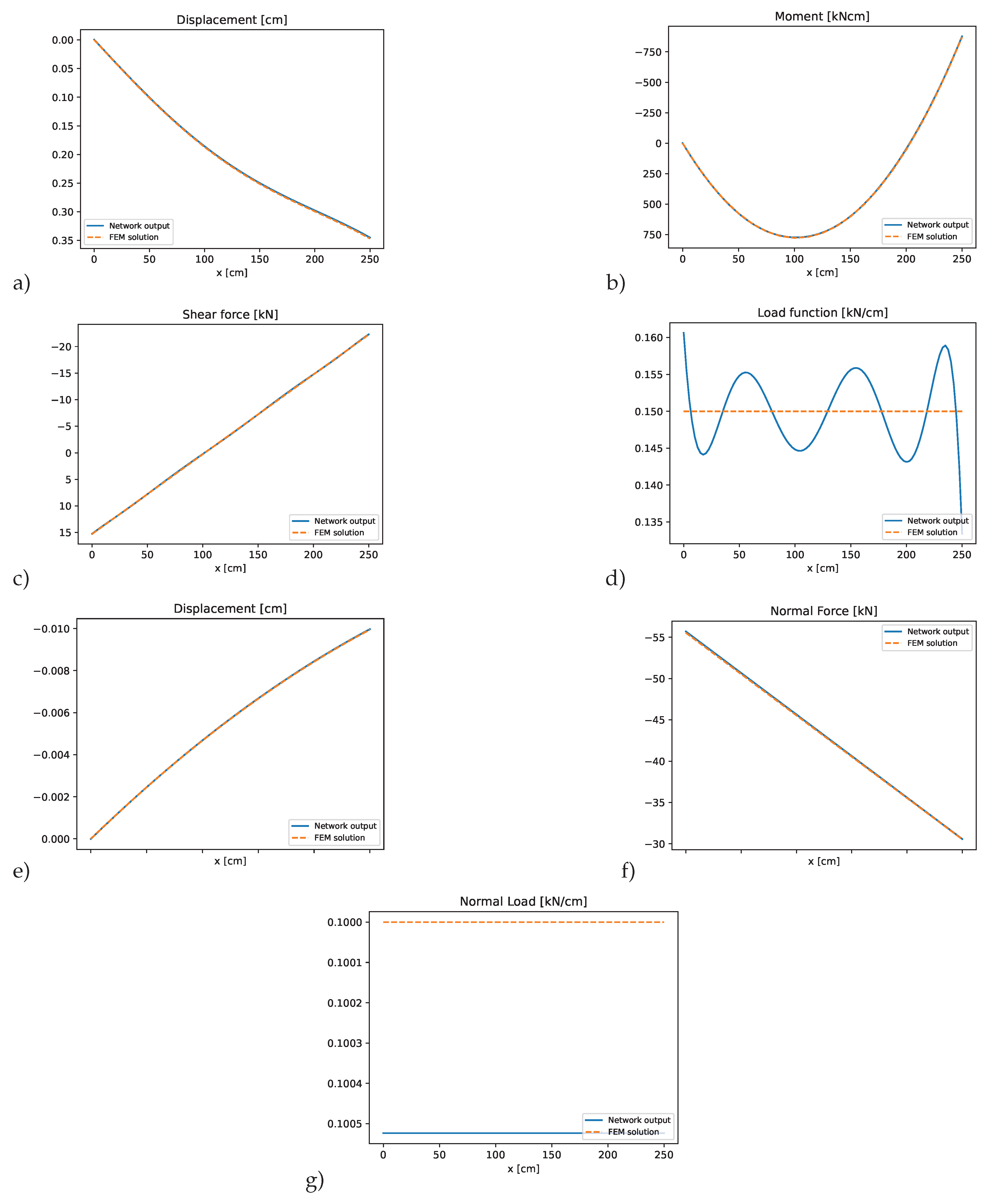
Figure 18.
PINN results for element 2 of the double-hinged frame: a) bending displacements, b) bending moment, c) shear force, d) predicted transverse load, e) axial displacements, f) normal force, g) predicted axial load compared to the finite element solution.
Figure 18.
PINN results for element 2 of the double-hinged frame: a) bending displacements, b) bending moment, c) shear force, d) predicted transverse load, e) axial displacements, f) normal force, g) predicted axial load compared to the finite element solution.
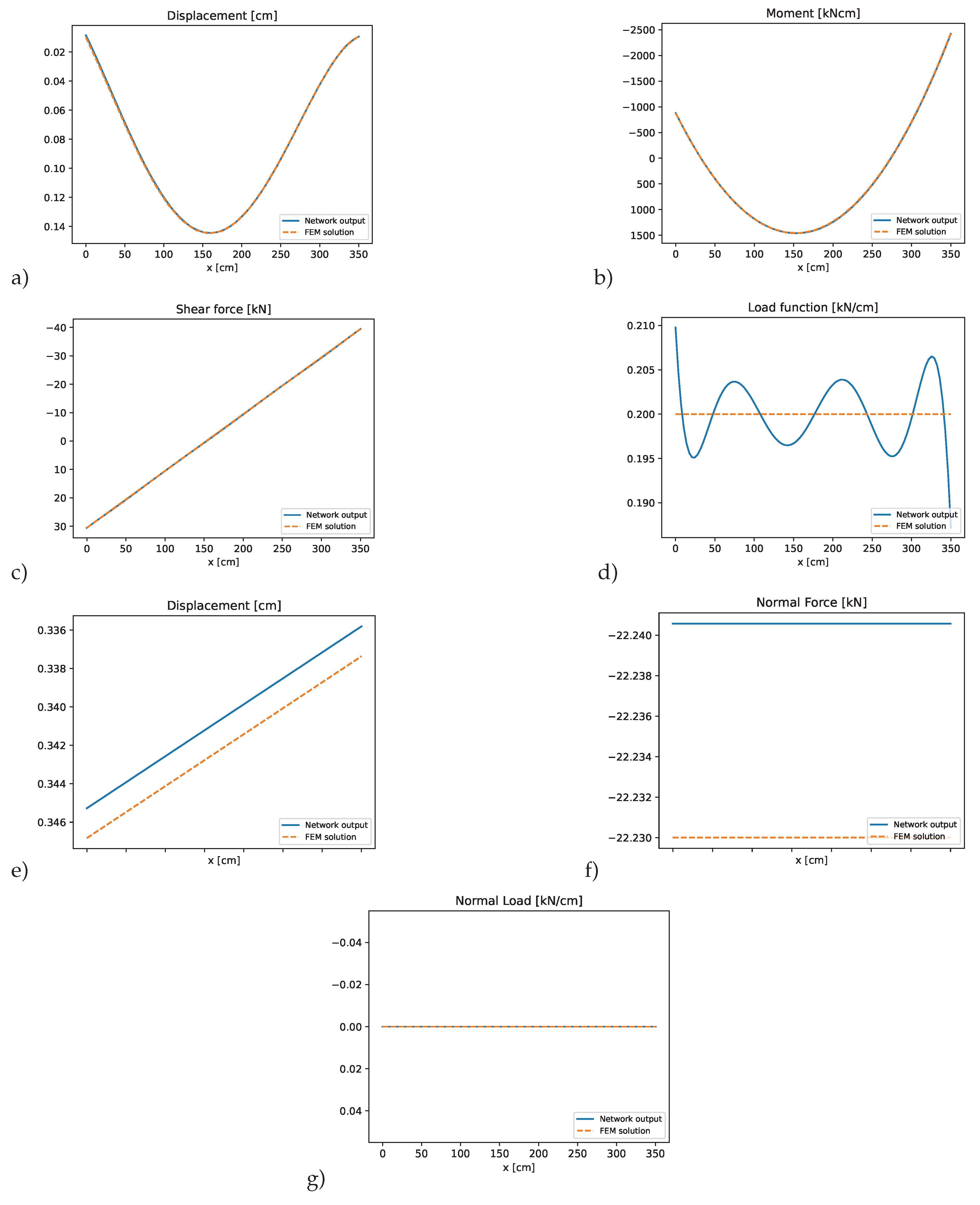
Figure 19.
PINN results for element 3 of the double-hinged frame: a) bending displacements, b) bending moment, c) shear force, d) predicted transverse load, e) axial displacements, f) normal force, g) predicted axial load compared to the finite element solution.
Figure 19.
PINN results for element 3 of the double-hinged frame: a) bending displacements, b) bending moment, c) shear force, d) predicted transverse load, e) axial displacements, f) normal force, g) predicted axial load compared to the finite element solution.
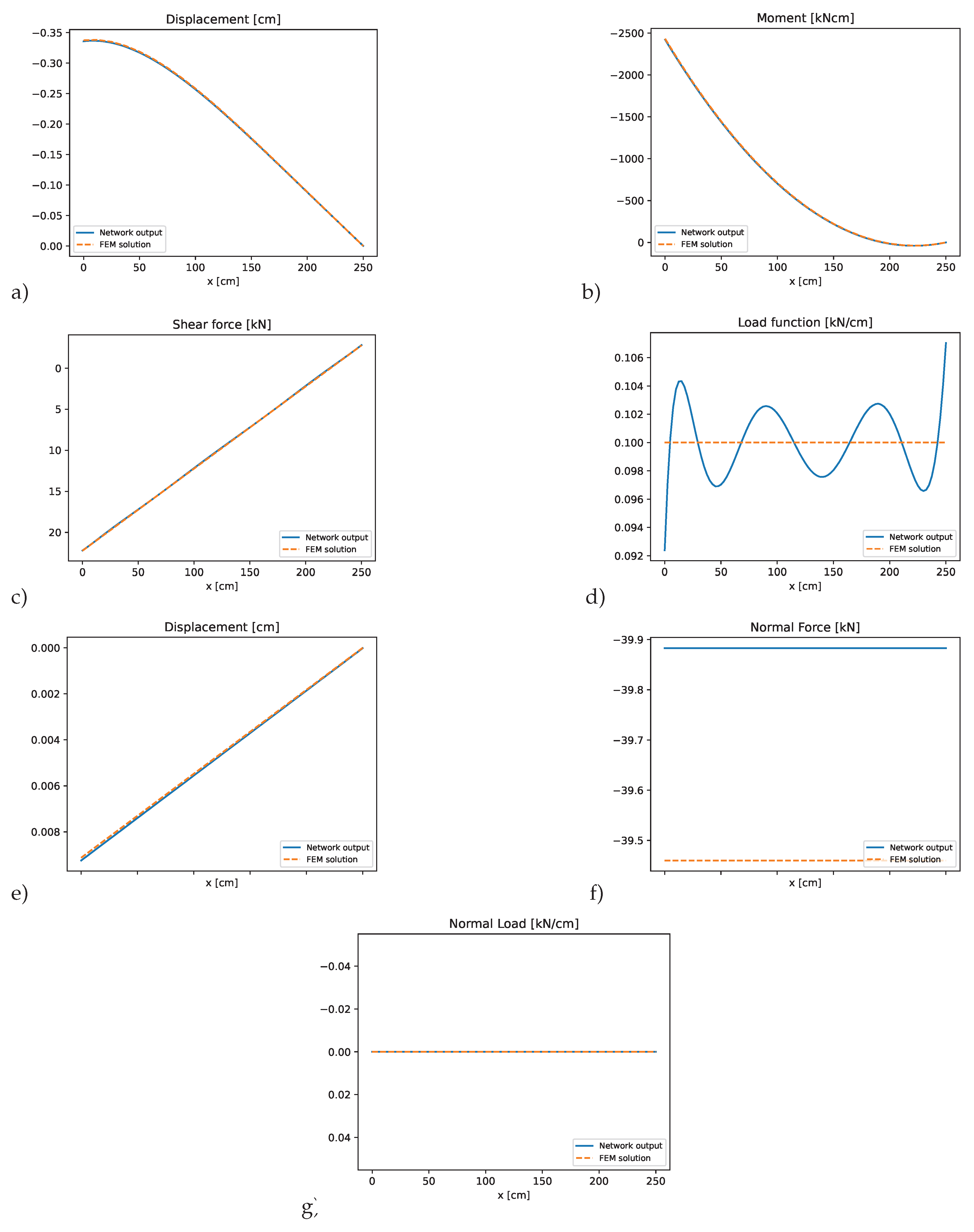
Figure 20 shows the optimization progress over 25,000 training epochs. For the first 17,000 epochs, the optimizer exhibits stable behavior while gradually exploring and minimizing the loss landscape. During this phase, both the physics and boundary condition losses decrease steadily. However, beyond 17,000 epochs, the optimization becomes increasingly unstable, with noticeable fluctuations in the total and component losses. This instability reflects the optimizer struggling to further minimize the loss or settling into local minima. At exactly 25,000 epochs, the optimization method is switched from Adam to L-BFGS, which leads to the prominent spike in the total loss observed at the end of the graph. This switch aims to refine the solution and improve convergence in the final training phase.
Within this example, it was observed that the PINN’s performance is highly sensitive to the choice of loss weights. Small changes in these weights had a noticeable impact on convergence and final accuracy. This highlights the importance of proper weight selection and suggests that future work should consider automated strategies for dynamically tuning loss weights during training. The weighting factors used in the example were applied uniformly across all elements k. For the physics contributions, the weights were set to
The boundary condition terms were weighted by
The weights for the coupling conditions were generally set to
However, four specific force conditions required significantly higher weighting to obtain a stable and accurate solution. In particular, the conditions enforcing equilibrium between the shear force at the end of element 1 and the normal force at the start of element 2, as well as between the normal force of element 2 and the shear force of element 3; these conditions were weighted with
Similarly, the conditions ensuring continuity between the normal force at the end of element 1 and the shear force at the start of element 2, as well as between the shear force at the end of element 2 and the normal force at the start of element 3, were weighted with
4. Discussion
Within the presented study, 2D frame structures which consists of two or three structural elements were analyzed using Physical Informed Neural Networks. The displacements in transverse and axial directions for each element were modeled separately by a single neural network with a single hidden layer. The investigations could show, that the obtained approximation was sufficiently accurate to represent the resulting internal forces and displacement functions. The coupling conditions between two or more elements and the boundary conditions at the supports of the structure were imposed in joined loss function for the training procedure by specific weighting factors. These weights were chosen by hand since they were found to have a substantial influence on the convergence behavior and final accuracy of the trained networks. Especially, the consideration of the axial displacements and forces in the rigid corners increased the manual effort to obtain optimal weighting factors.
It is imperative to acknowledge that while the presented optimization strategies led to satisfactory results, they are not guaranteed to be optimal. It is noteworthy that different training schemes and hyper-parameter configurations may yield improved performance, and the approaches adopted in this study were chosen based on empirical observations rather than exhaustive tuning. In the context of future research efforts, it would be advantageous to integrate a method that jointly optimizes the loss weights in parallel with the network parameters. Such an approach could help to shape a more favorable loss landscape and guide the optimization process more effectively toward meaningful minima. Such an automatic adaptation scheme seems to be the most relevant issue in the opinion of the authors to extend the presented approach to more complex structures and even for a full 3D representation.
5. Conclusions
The presented PINN approach could be an interesting alternative to traditional finite elements for the analysis of frame structures, since it allows a more flexible modeling of the load functions and the consideration of varying cross section properties of the individual structural elements. However, the assembling of the individual networks within a joined training process will increase the number of optimization parameters and requires efficient algorithms for the training. Since the displacements are represented for one structural element by continuous approximation functions the representation of discrete loads should be realized by subdividing the structure to further elements and consider the discrete loads directly at the connection nodes and the coupling conditions.
Author Contributions
Conceptualization, L.L. and T.M.; methodology, F.D., L.L. and T.M.; software, F.D. and L.L.; validation, F.D. and L.L.; formal analysis, F.D.; investigation, F.D.; resources, F.D.; data curation, F.D.; writing—original draft preparation, F.D.; writing—review and editing, L.L., T.M. and C.K.; visualization, F.D.; supervision, L.L., T.M. and C.K.; project administration, T.M.; funding acquisition, C.K. All authors have read and agreed to the published version of the manuscript.
Funding
This research has been supported by the German Research Foundation (DFG) through the project DIVING within the priority program SPP 100+.
Institutional Review Board Statement
Not applicable
Informed Consent Statement
Not applicable
Data Availability Statement
The complete python calculation files including all presented results are available in the publicly accessible repository https://refodat.de/ at the DOI xxx (will be available soon).
Acknowledgments
We acknowledge support for the publication costs from the Open Access Publication Fund of Bauhaus Universität Weimar and the German Research Foundation (DFG).
Conflicts of Interest
The authors declare no conflicts of interest.
Abbreviations
The following abbreviations are used in this manuscript:
| PDE | Partial differential equation |
| ML | Machine learning |
| NN | Neural network |
| ANN | Artifical neural network |
| FEM | Finite element method |
| PINN | Physics informed neural network |
| Adam | Adaptive Moment Estimation |
| L-BFGS | Limited-memory Broyden-Fletcher-Goldfarb-Shanno |
References
- Raissi, M.; Perdikaris, P.; Karniadakis, G. Physics-informed neural networks: A deep learning framework for solving forward and inverse problems involving nonlinear partial differential equations. Journal of Computational Physics 2019, 378, 686–707. [Google Scholar] [CrossRef]
- Karniadakis, G.E.; Kevrekidis, I.G.; Lu, L.; Perdikaris, P.; Wang, S.; Yang, L. Physics-informed machine learning. Nature Reviews Physics 2021, 3, 422–440. [Google Scholar] [CrossRef]
- Cuomo, S.; Di Cola, V.S.; Giampaolo, F.; Rozza, G.; Raissi, M.; Piccialli, F. Scientific machine learning through physics–informed neural networks: Where we are and what’s next. Journal of Scientific Computing 2022, 92, 88. [Google Scholar] [CrossRef]
- Bai, J.; Rabczuk, T.; Gupta, A.; Alzubaidi, L.; Gu, Y. A physics-informed neural network technique based on a modified loss function for computational 2D and 3D solid mechanics. Computational Mechanics 2023, 71, 543–562. [Google Scholar] [CrossRef]
- Fallah, A.; Aghdam, M.M. Physics-informed neural network for bending and free vibration analysis of three-dimensional functionally graded porous beam resting on elastic foundation. Engineering with Computers 2024, 40, 437–454. [Google Scholar] [CrossRef]
- Kapoor, T.; Wang, H.; Núñez, A.; Dollevoet, R. Physics-informed neural networks for solving forward and inverse problems in complex beam systems. IEEE Transactions on Neural Networks and Learning Systems 2023, 35, 5981–5995. [Google Scholar] [CrossRef]
- Al-Adly, A.I.; Kripakaran, P. Physics-informed neural networks for structural health monitoring: a case study for Kirchhoff–Love plates. Data-Centric Engineering 2024, 5, e6. [Google Scholar] [CrossRef]
- Lippold, L.; Rödiger, N.; Most, T.; Könke, C. Identifikation inhomogener Materialeigenschaften von Flächentragwerken mit Physics Informed Neural Networks. In 15. Fachtagung Baustatik – Baupraxis, Hamburg, Germany, 4-5 March, 2024; 2024.
- Guo, H.; Zhuang, X.; Rabczuk, T. A deep collocation method for the bending analysis of Kirchhoff plate. arXiv 2021, arXiv:2102.02617 2021. [Google Scholar] [CrossRef]
- Xu, C.; Cao, B.T.; Yuan, Y.; Meschke, G. Transfer learning based physics-informed neural networks for solving inverse problems in engineering structures under different loading scenarios. Computer Methods in Applied Mechanics and Engineering 2023, 405, 115852. [Google Scholar] [CrossRef]
- Bastek, J.H.; Kochmann, D.M. Physics-informed neural networks for shell structures. European Journal of Mechanics-A/Solids 2023, 97, 104849. [Google Scholar] [CrossRef]
- Haghighat, E.; Raissi, M.; Moure, A.; Gomez, H.; Juanes, R. A physics-informed deep learning framework for inversion and surrogate modeling in solid mechanics. Computer Methods in Applied Mechanics and Engineering 2021, 379, 113741. [Google Scholar] [CrossRef]
- Wu, L.; Kilingar, N.G.; Noels, L.; et al. A recurrent neural network-accelerated multi-scale model for elasto-plastic heterogeneous materials subjected to random cyclic and non-proportional loading paths. Computer Methods in Applied Mechanics and Engineering 2020, 369, 113234. [Google Scholar] [CrossRef]
- Maia, M.; Rocha, I.B.; Kerfriden, P.; van der Meer, F.P. Physically recurrent neural networks for path-dependent heterogeneous materials: Embedding constitutive models in a data-driven surrogate. Computer Methods in Applied Mechanics and Engineering 2023, 407, 115934. [Google Scholar] [CrossRef]
- Goswami, S.; Anitescu, C.; Chakraborty, S.; Rabczuk, T. Transfer learning enhanced physics informed neural network for phase-field modeling of fracture. Theoretical and Applied Fracture Mechanics 2020, 106, 102447. [Google Scholar] [CrossRef]
- Zheng, B.; Li, T.; Qi, H.; Gao, L.; Liu, X.; Yuan, L. Physics-informed machine learning model for computational fracture of quasi-brittle materials without labelled data. International Journal of Mechanical Sciences 2022, 223, 107282. [Google Scholar] [CrossRef]
- Samaniego, E.; Anitescu, C.; Goswami, S.; Nguyen-Thanh, V.M.; Guo, H.; Hamdia, K.; Zhuang, X.; Rabczuk, T. An energy approach to the solution of partial differential equations in computational mechanics via machine learning: Concepts, implementation and applications. Computer Methods in Applied Mechanics and Engineering 2020, 362, 112790. [Google Scholar] [CrossRef]
- Jagtap, A.D.; Karniadakis, G.E. Extended physics-informed neural networks (XPINNs): A generalized space-time domain decomposition based deep learning framework for nonlinear partial differential equations. Communications in Computational Physics 2020, 28. [Google Scholar]
- Grossmann, T.G.; Komorowska, U.J.; Latz, J.; Schönlieb, C.B. Can physics-informed neural networks beat the finite element method? IMA Journal of Applied Mathematics 2024, 89, 143–174. [Google Scholar] [CrossRef]
- Meethal, R.E.; Kodakkal, A.; Khalil, M.; Ghantasala, A.; Obst, B.; Bletzinger, K.U.; Wüchner, R. Finite element method-enhanced neural network for forward and inverse problems. Advanced modeling and simulation in engineering sciences 2023, 10, 6. [Google Scholar] [CrossRef]
- Hu, Z.; Shukla, K.; Karniadakis, G.E.; Kawaguchi, K. Tackling the curse of dimensionality with physics-informed neural networks. Neural Networks 2024, 176, 106369. [Google Scholar] [CrossRef]
- Guo, X.Y.; Fang, S.E. Structural parameter identification using physics-informed neural networks. Measurement 2023, 220, 113334. [Google Scholar] [CrossRef]
- Zhang, E.; Dao, M.; Karniadakis, G.E.; Suresh, S. Analyses of internal structures and defects in materials using physics-informed neural networks. Science advances 2022, 8, eabk0644. [Google Scholar] [CrossRef] [PubMed]
- Zhou, W.; Xu, Y. Damage identification for plate structures using physics-informed neural networks. Mechanical Systems and Signal Processing 2024, 209, 111111. [Google Scholar] [CrossRef]
- Faroughi, S.; Darvishi, A.; Rezaei, S. On the order of derivation in the training of physics-informed neural networks: case studies for non-uniform beam structures. Acta Mechanica 2023, 234, 5673–5695. [Google Scholar] [CrossRef]
- Gere, J.; Timoshenko, S. Mechanics of Materials; PWS: Boston, MA, 1997. [Google Scholar]
- Wang, S.; Sankaran, S.; Wang, H.; Perdikaris, P. An Expert’s Guide to Training Physics-informed Neural Networks, 2023, [arXiv:cs.LG/2308.08468].
- Yu, J.; Spiliopoulos, K. Normalization effects on deep neural networks, 2022, [arXiv:cs.LG/2209.01018].
- Paszke, A.; Gross, S.; Massa, F.; Lerer, A.; Bradbury, J.; Chanan, G.; Killeen, T.; Lin, Z.; Gimelshein, N.; Antiga, L.; et al. PyTorch: An Imperative Style, High-Performance Deep Learning Library. In Advances in Neural Information Processing Systems 32; Curran Associates, Inc., 2019; pp. 8024–8035.
- Kingma, D.P.; Ba, J. Adam: A Method for Stochastic Optimization. International Conference on Learning Representations (ICLR) 2015. [Google Scholar]
- Liu, D.C.; Nocedal, J. On the limited memory BFGS method for large scale optimization. Mathematical programming 1989, 45, 503–528. [Google Scholar] [CrossRef]
- Dlubal Software GmbH. RSTAB 9 — User’s Manual: Modeling and Calculation of Beam, Frame, and Truss Structures. Tiefenbach, Germany, version 9 ed., 2025.
Figure 1.
Scheme showing variables of the general bending beam setup. Loading q and bending stiffness are arbitrary functions of coordinate x. The supports can be of various kinds.
Figure 1.
Scheme showing variables of the general bending beam setup. Loading q and bending stiffness are arbitrary functions of coordinate x. The supports can be of various kinds.
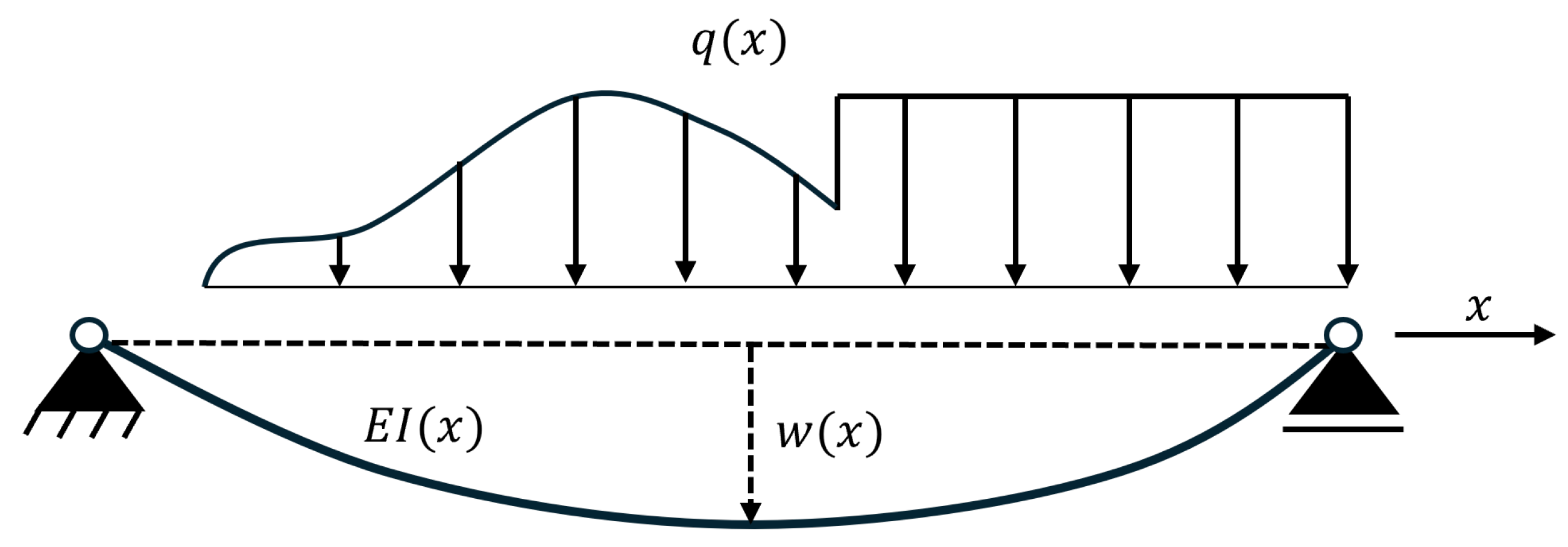
Figure 2.
Scheme showing variables for general rod setup. and the axial load n are general functions of the coordinate x.
Figure 2.
Scheme showing variables for general rod setup. and the axial load n are general functions of the coordinate x.
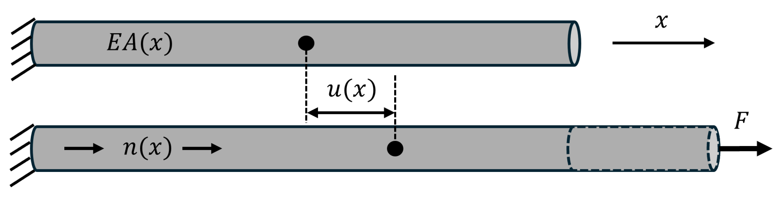
Figure 3.
Network architecture representing the bending deflections of a single beam on the nondimensional length scale . are the linear weights of the input and hidden layers of the network and and are the corresponding biases and activation functions of the neurons.
Figure 3.
Network architecture representing the bending deflections of a single beam on the nondimensional length scale . are the linear weights of the input and hidden layers of the network and and are the corresponding biases and activation functions of the neurons.
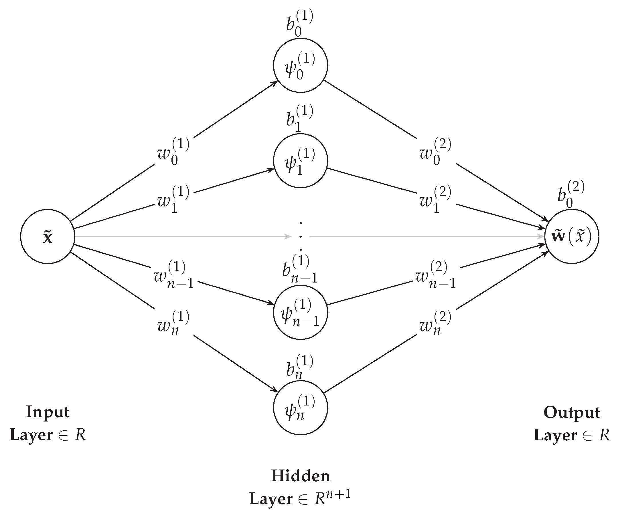
Figure 4.
PINN training scheme for an example structure with two elements by considering loss function terms for the physics , for the boundary conditions for each element as well as for the coupling conditions between the two elements.
Figure 4.
PINN training scheme for an example structure with two elements by considering loss function terms for the physics , for the boundary conditions for each element as well as for the coupling conditions between the two elements.
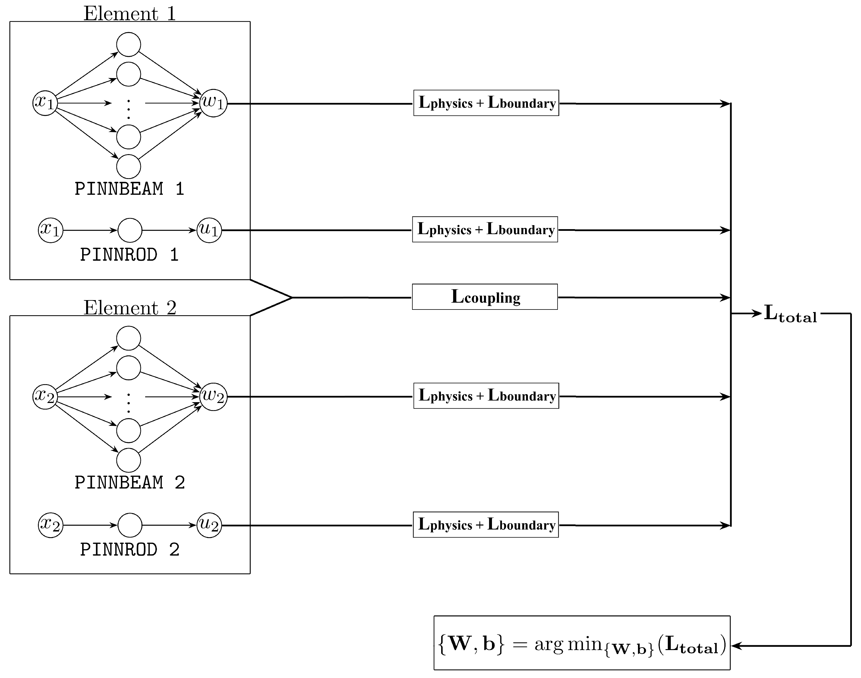
Figure 5.
Cantilever beam with decreasing bending stiffness according to Equation (29).
Figure 5.
Cantilever beam with decreasing bending stiffness according to Equation (29).
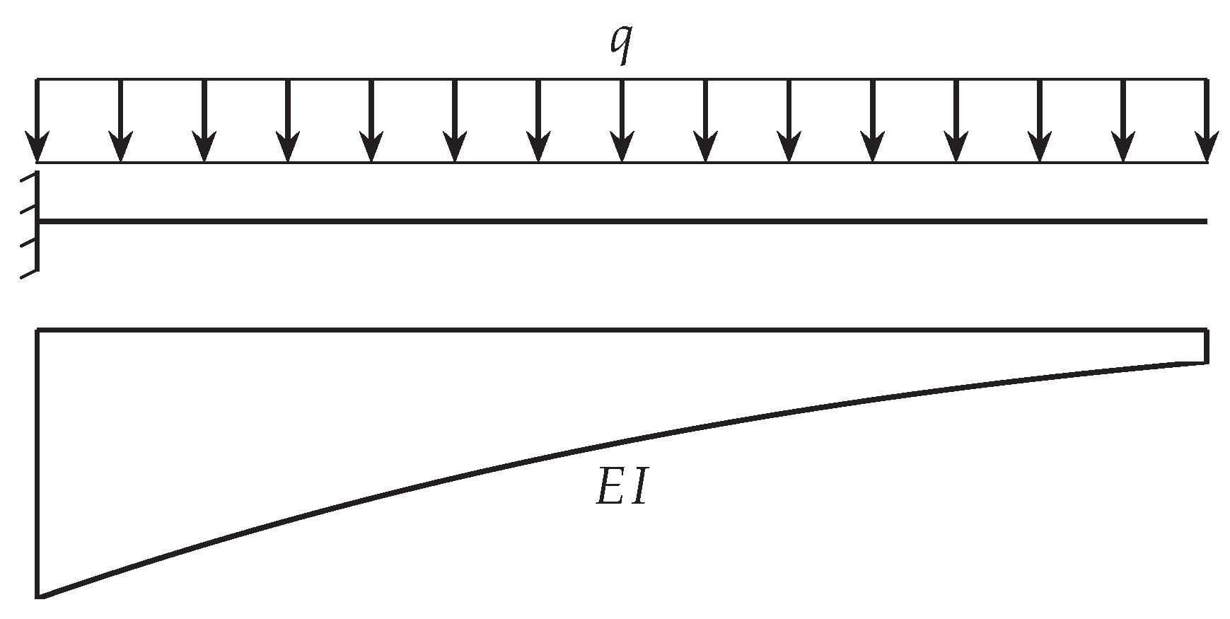
Figure 6.
PINN results for a cantilever beam with varying stiffness: a) displacements, b) bending moment, c) shear force, d) predicted load compared to the finite element solution.
Figure 6.
PINN results for a cantilever beam with varying stiffness: a) displacements, b) bending moment, c) shear force, d) predicted load compared to the finite element solution.
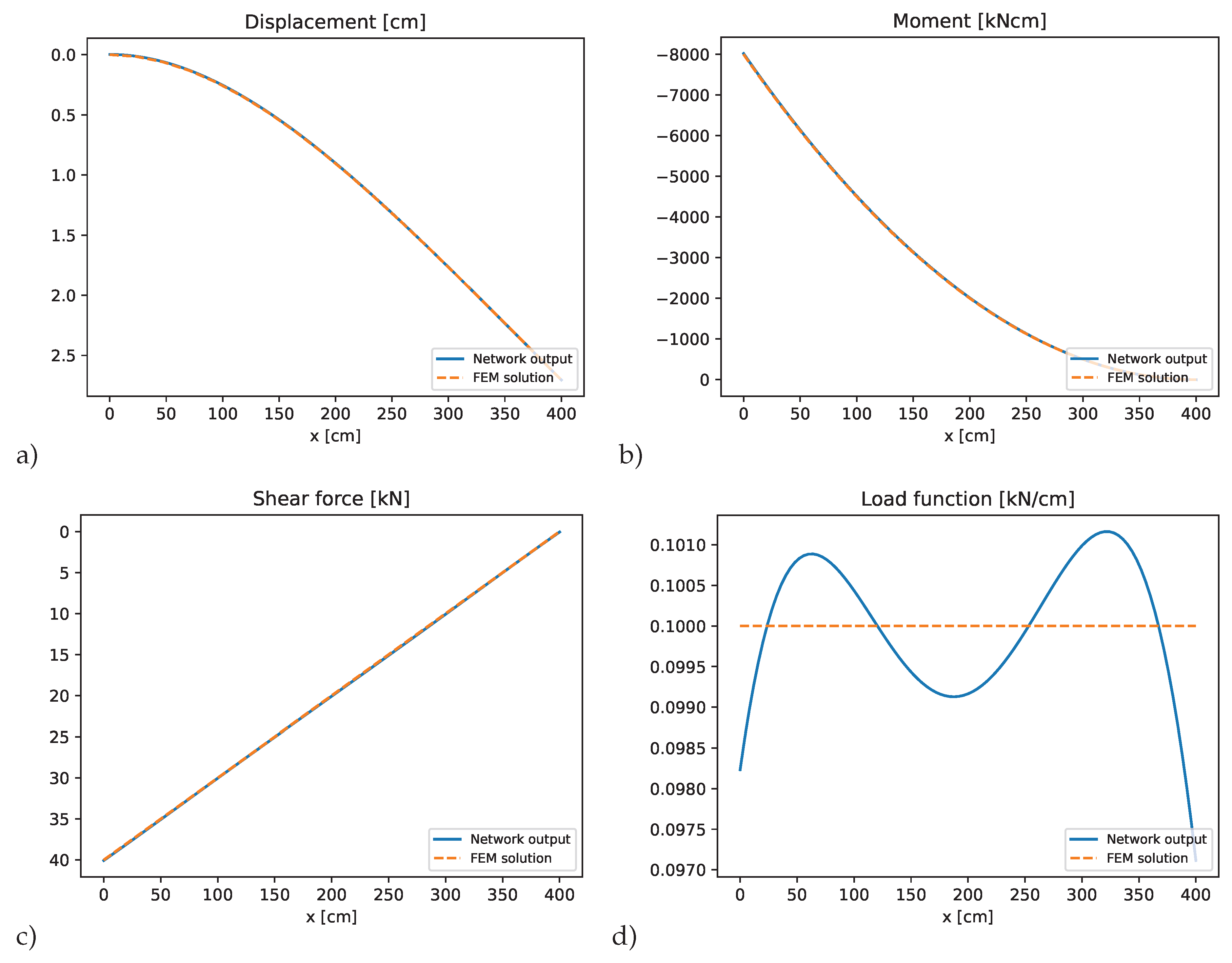
Figure 7.
Optimization convergence history of the logarithmic total loss for the cantilever beam with varying stiffness.
Figure 7.
Optimization convergence history of the logarithmic total loss for the cantilever beam with varying stiffness.
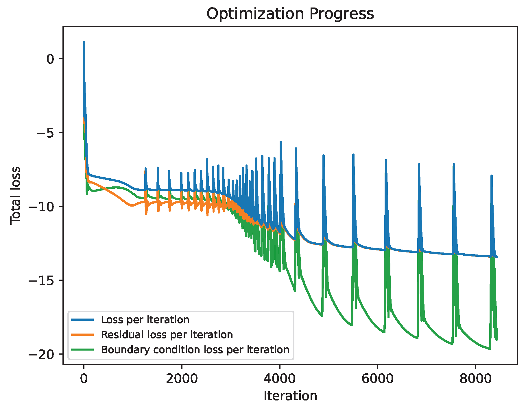
Figure 8.
Simply supported beam with concentrated load.
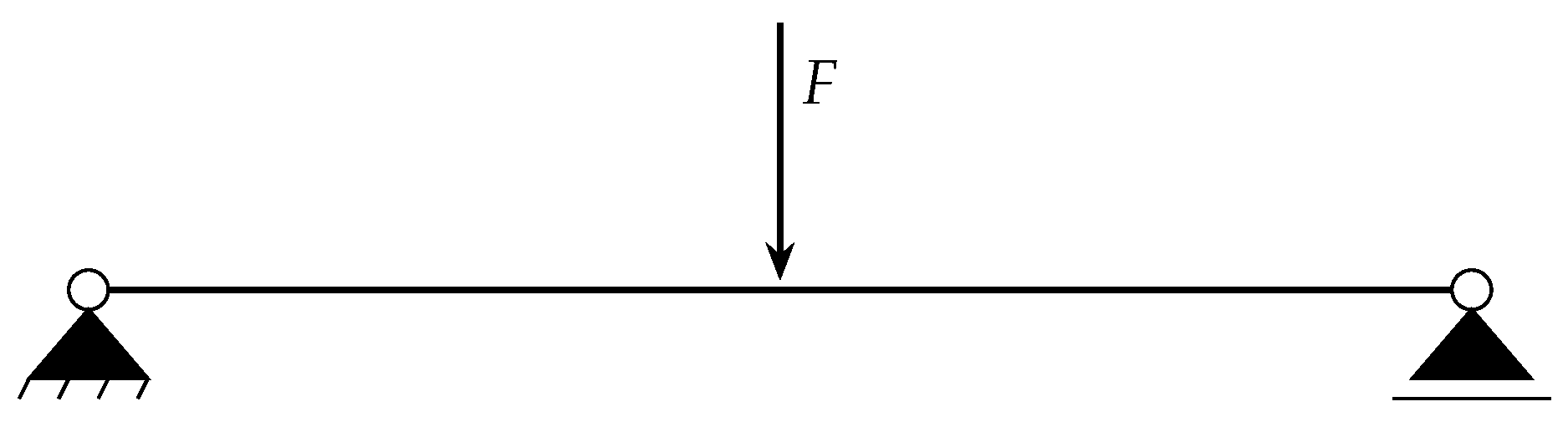
Figure 9.
PINN results for a simply supported beam with concentrated load: a) displacements, b) bending moment, c) shear force, d) predicted load compared to the finite element solution.
Figure 9.
PINN results for a simply supported beam with concentrated load: a) displacements, b) bending moment, c) shear force, d) predicted load compared to the finite element solution.
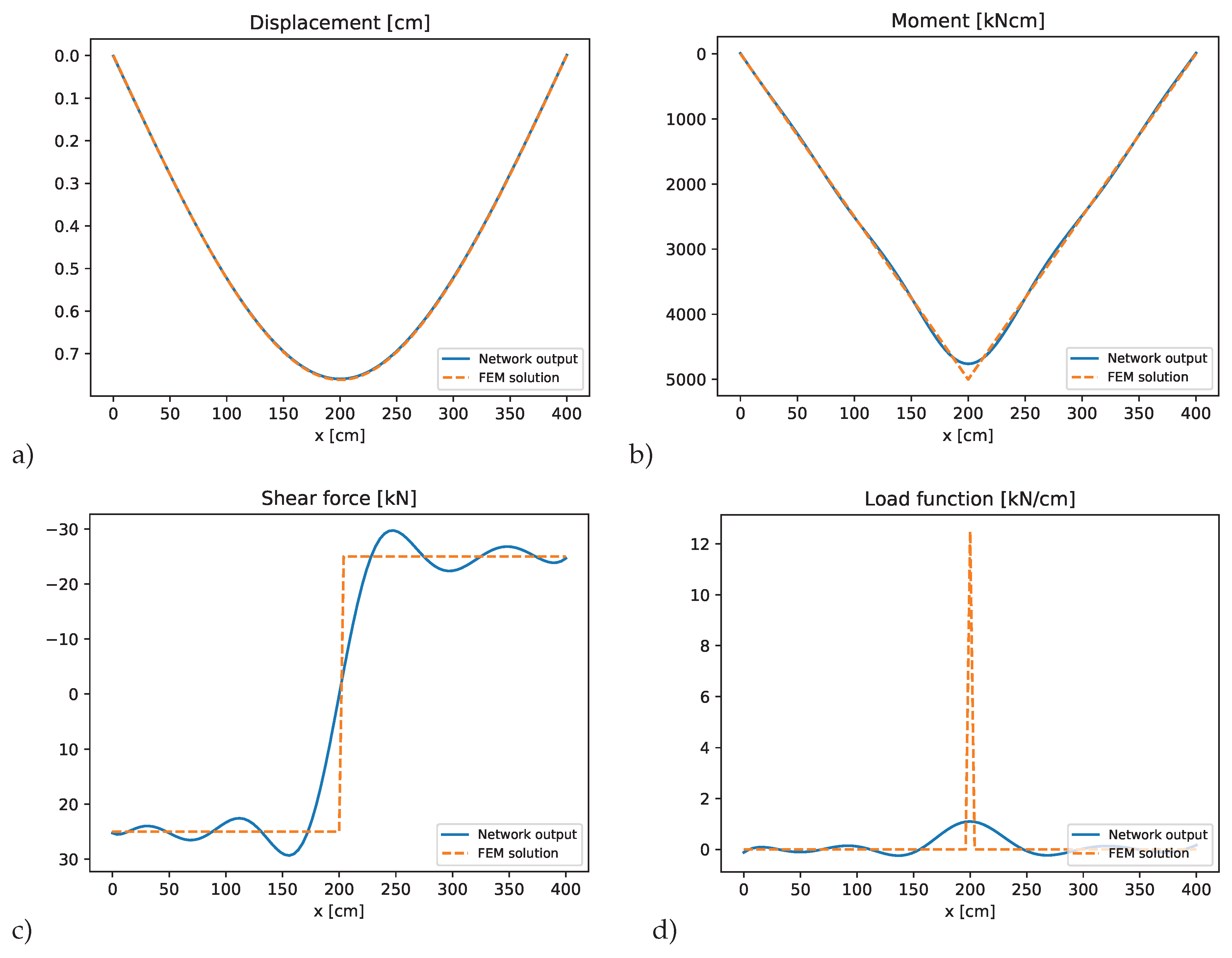
Figure 10.
Optimization convergence history of the logarithmic total loss for the simply supported beam with concentrated load
Figure 10.
Optimization convergence history of the logarithmic total loss for the simply supported beam with concentrated load
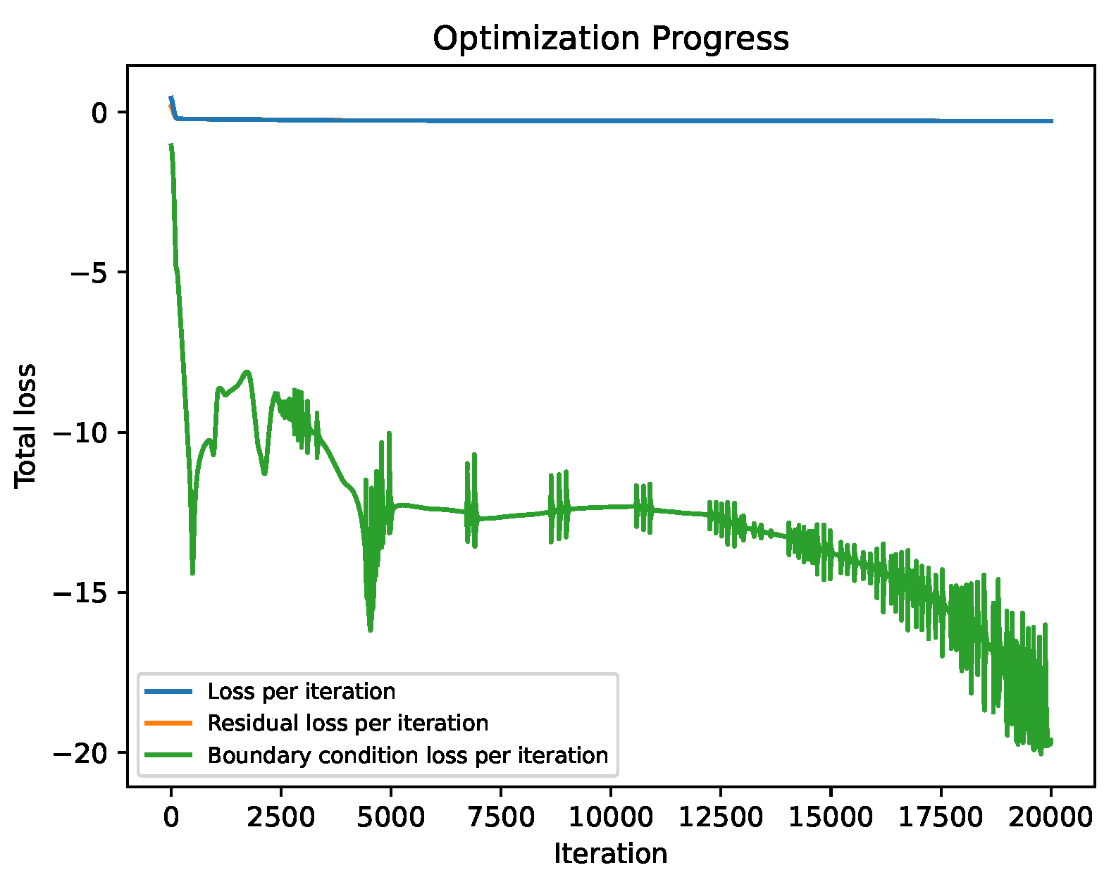
Figure 11.
T-structure consisting of three beam elements
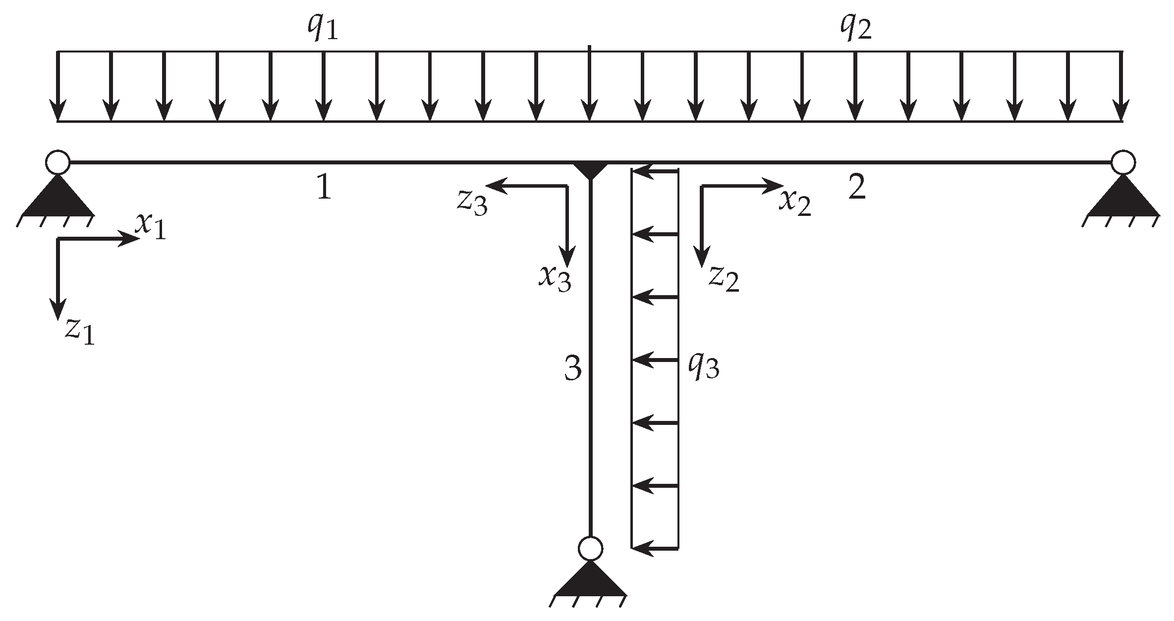
Figure 12.
PINN results for element 1 of the T-structure: a) bending displacements, b) bending moment, c) shear force, d) predicted transverse load, e) axial displacements, f) normal force compared to the finite element solution.
Figure 12.
PINN results for element 1 of the T-structure: a) bending displacements, b) bending moment, c) shear force, d) predicted transverse load, e) axial displacements, f) normal force compared to the finite element solution.
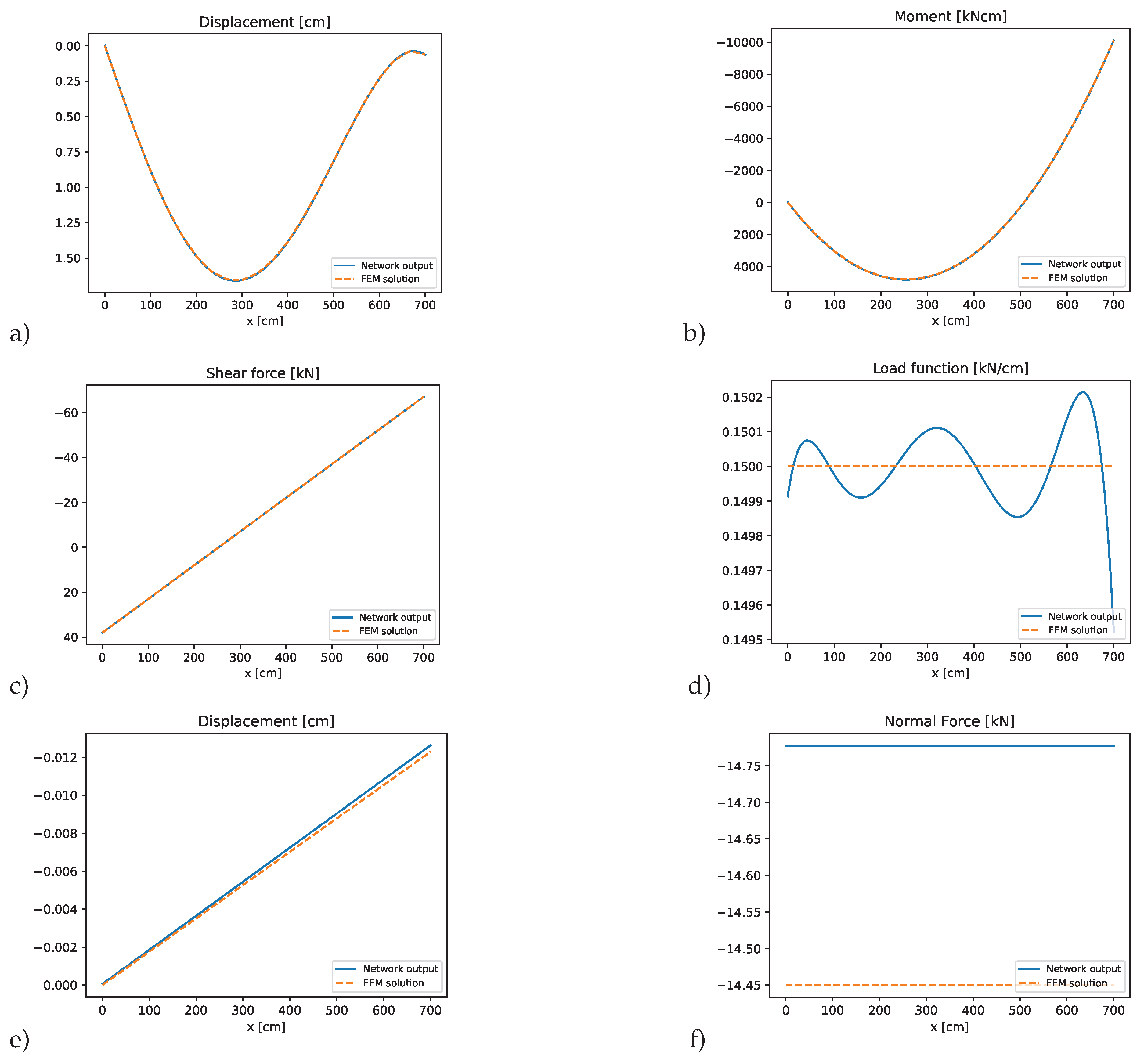
Figure 13.
PINN results for element 2 of the T-structure: a) bending displacements, b) bending moment, c) shear force, d) predicted transverse load, e) axial displacements, f) normal force compared to the finite element solution.
Figure 13.
PINN results for element 2 of the T-structure: a) bending displacements, b) bending moment, c) shear force, d) predicted transverse load, e) axial displacements, f) normal force compared to the finite element solution.
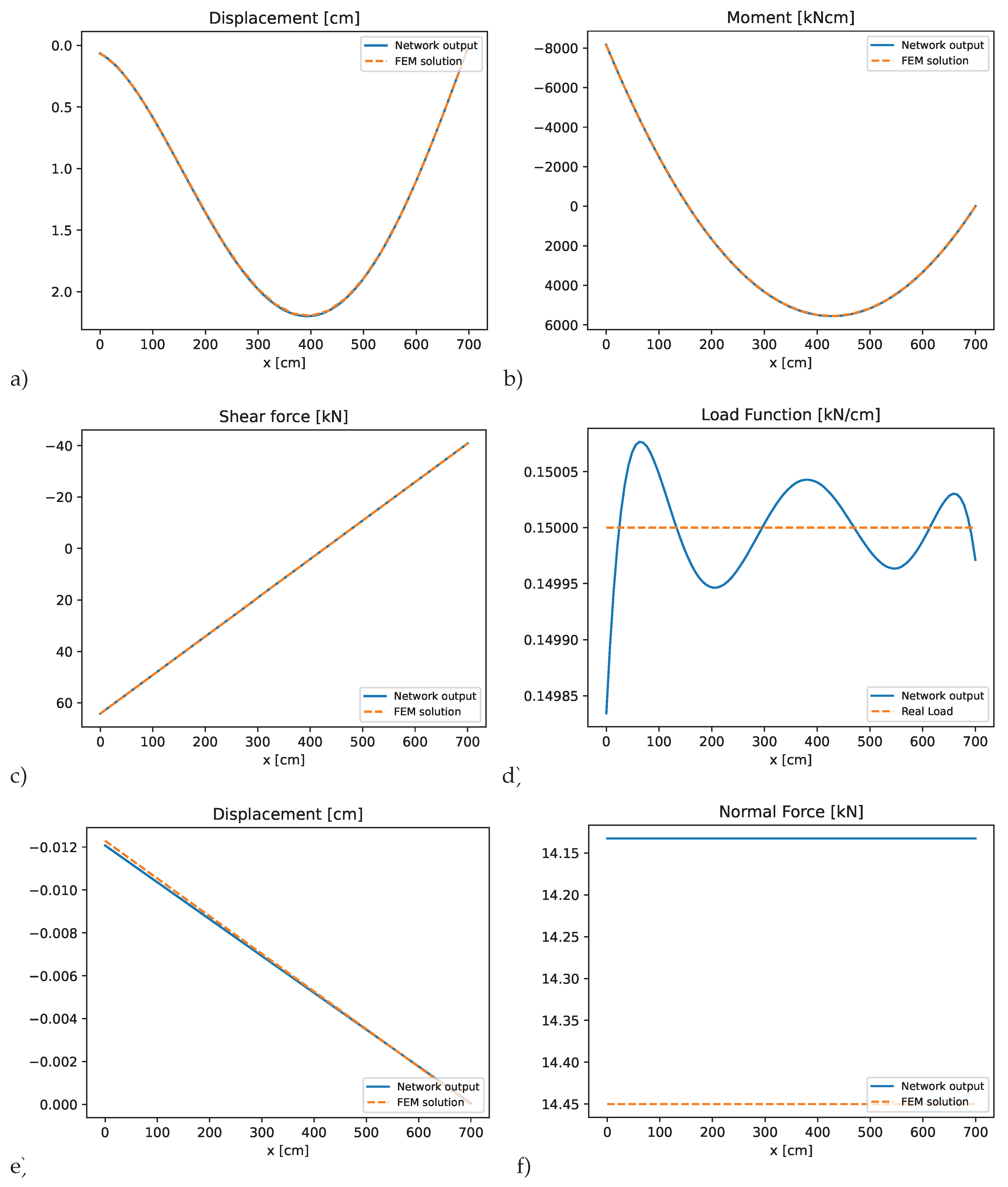
Figure 14.
PINN results for element 3 of the T-structure: a) bending displacements, b) bending moment, c) shear force, d) predicted transverse load, e) axial displacements, f) normal force compared to the finite element solution.
Figure 14.
PINN results for element 3 of the T-structure: a) bending displacements, b) bending moment, c) shear force, d) predicted transverse load, e) axial displacements, f) normal force compared to the finite element solution.
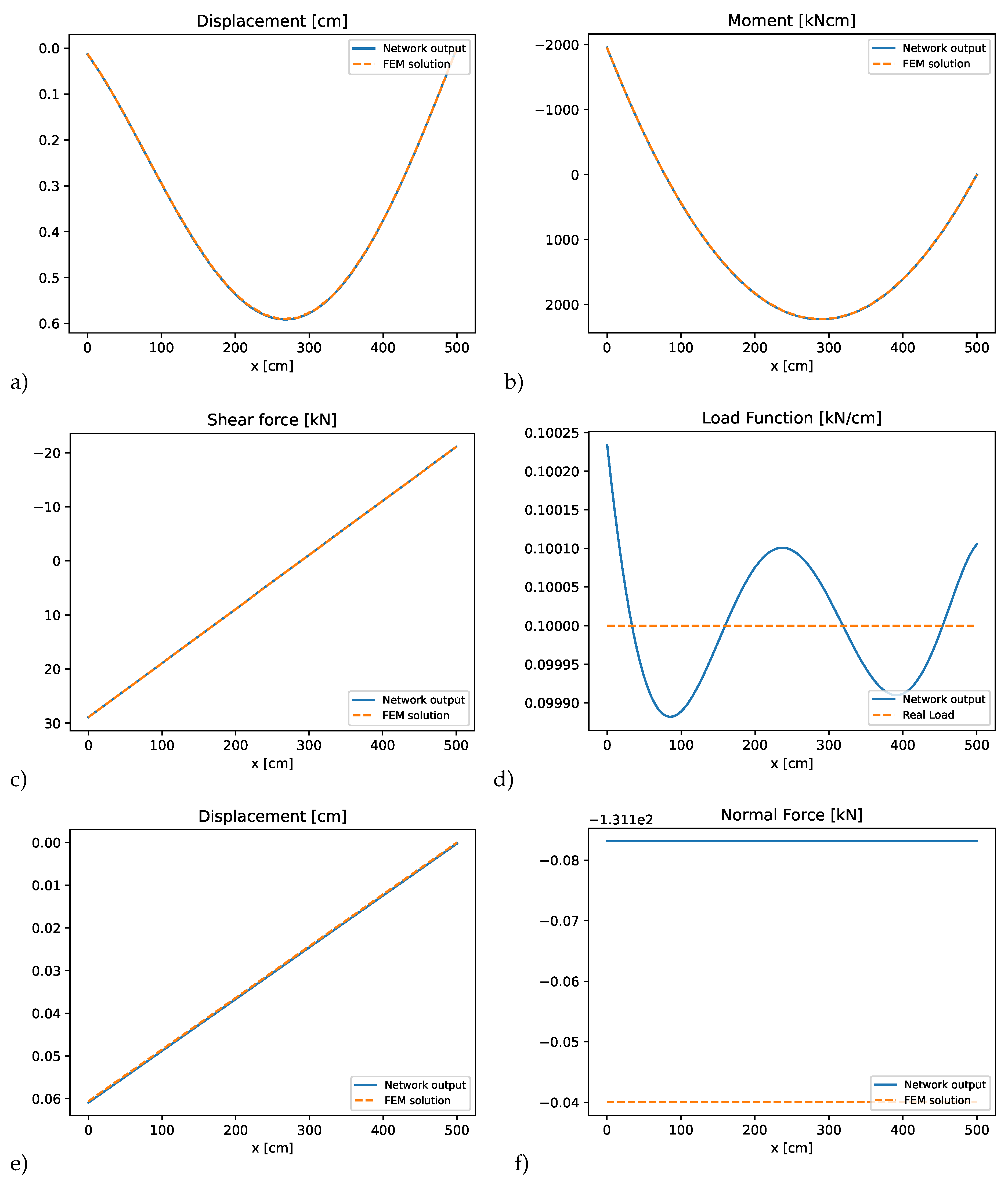
Figure 15.
Optimization convergence history of the logarithmic total loss for the T-structure.
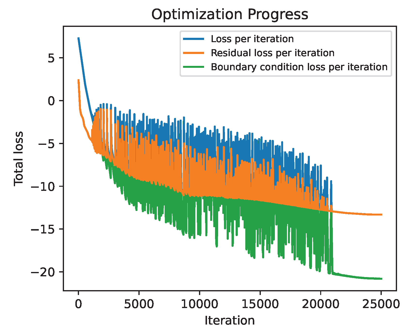
Figure 16.
Double-hinged frame structure.
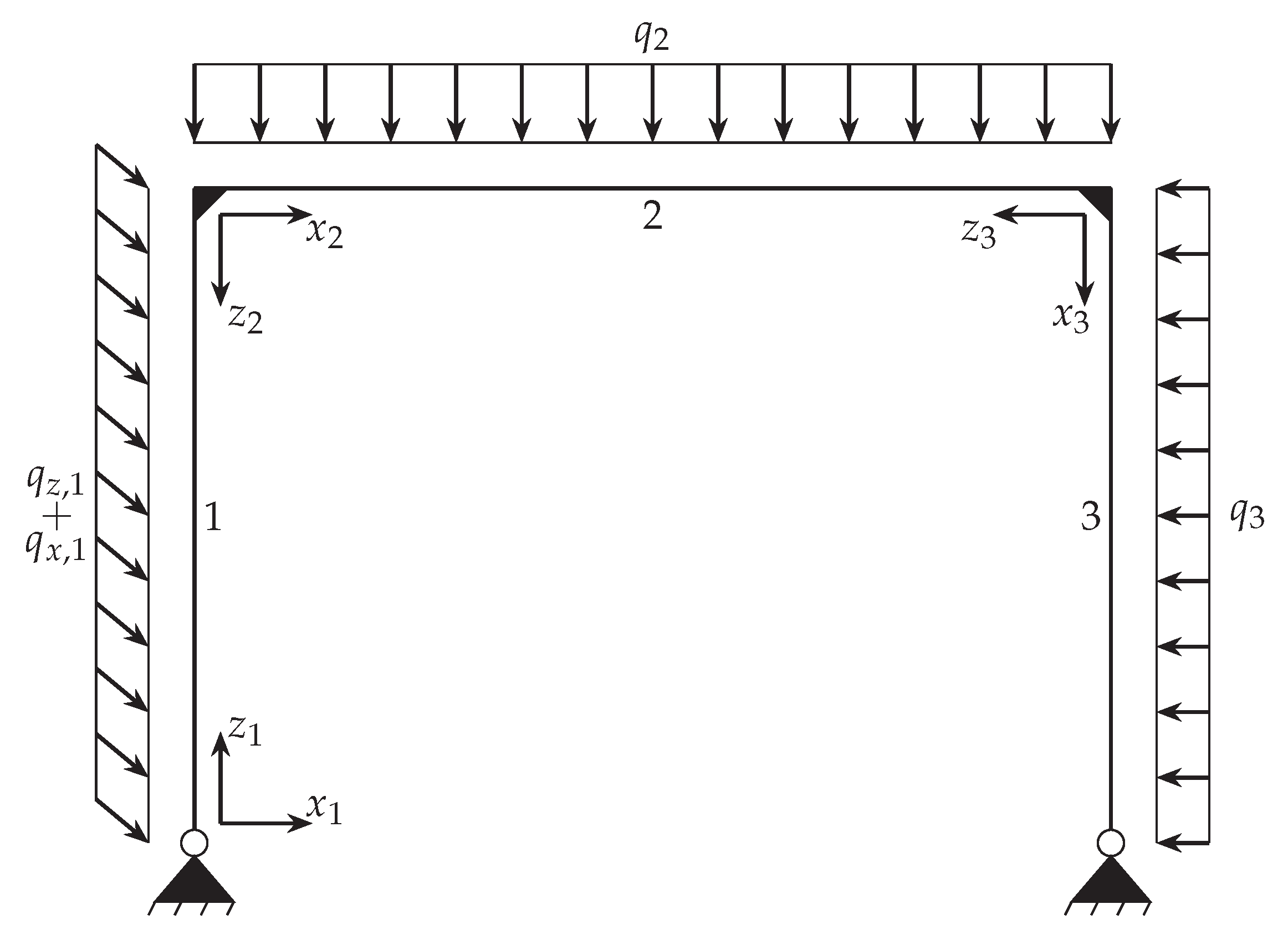
Figure 20.
Optimization convergence history of the logarithmic total loss for the double-hinged frame.
Figure 20.
Optimization convergence history of the logarithmic total loss for the double-hinged frame.
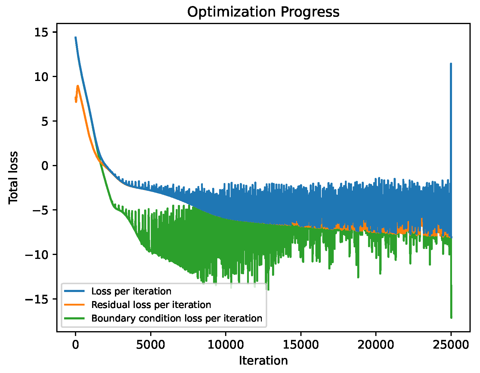

Table 1.
Boundary conditions for bending and axial displacements for different support types.
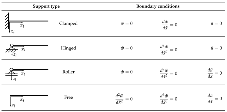
Table 2.
Different examples for the connection of structural elements and the corresponding coupling conditions: a) two beams with rigid connection, b) two beams with hinged connection, c) rigid corner with 2 elements, d) rigid corner with 3 elements.
Table 2.
Different examples for the connection of structural elements and the corresponding coupling conditions: a) two beams with rigid connection, b) two beams with hinged connection, c) rigid corner with 2 elements, d) rigid corner with 3 elements.
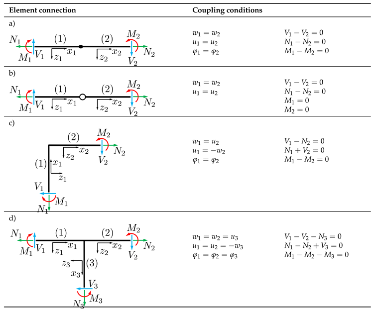
Table 3.
System properties of the cantilever beam with decreasing bending stiffness.
| Property | Unit | Value | |
|---|---|---|---|
| Young’s modulus E | kN/cm² | ||
| Beam length L | cm | ||
| Beam width b | cm | 10.0 | |
| Beam heigth left side | cm | 20.0 | |
| Beam heigth right side | cm | 15.0 | |
| Constant load q | kN/cm | 0.10 | |
Table 4.
System properties of the simply supported beam with concentrated load.
| Property | Unit | Value | |
|---|---|---|---|
| Young’s modulus E | kN/cm² | ||
| Beam length L | cm | ||
| Area moment of inertia | cm4 | 4170.0 | |
| Concentrated load F | kN | 50.0 | |
Table 5.
System properties of the T-structure with multiple beams.
| Property | Unit | Value | |
|---|---|---|---|
| Young’s modulus E | kN/cm² | ||
| Beam length , | cm | ||
| Beam length | cm | ||
| Area moment of inertia , | cm4 | 4917.0 | |
| Area moment of inertia | cm4 | 4170.0 | |
| Cross section area , | cm² | 39.15 | |
| Cross section area | cm² | 51.46 | |
| Constant load , | kN/cm | 0.15 | |
| Constant load | kN/cm | 0.10 | |
Table 6.
System properties of the double-hinged frame structure.
| Property | Unit | Value | |
|---|---|---|---|
| Young’s modulus E | kN/cm² | ||
| Beam length , | cm | ||
| Beam length | cm | ||
| Area moment of inertia , | cm4 | 4170.0 | |
| Area moment of inertia | cm4 | 4917.0 | |
| Cross section area , | cm² | 51.46 | |
| Cross section area | cm² | 39.15 | |
| Constant load | kN/cm | 0.15 | |
| Constant load | kN/cm | 0.10 | |
| Constant load | kN/cm | 0.20 | |
| Constant load | kN/cm | 0.10 | |
Disclaimer/Publisher’s Note: The statements, opinions and data contained in all publications are solely those of the individual author(s) and contributor(s) and not of MDPI and/or the editor(s). MDPI and/or the editor(s) disclaim responsibility for any injury to people or property resulting from any ideas, methods, instructions or products referred to in the content. |
© 2025 by the authors. Licensee MDPI, Basel, Switzerland. This article is an open access article distributed under the terms and conditions of the Creative Commons Attribution (CC BY) license (http://creativecommons.org/licenses/by/4.0/).
Copyright: This open access article is published under a Creative Commons CC BY 4.0 license, which permit the free download, distribution, and reuse, provided that the author and preprint are cited in any reuse.


