Submitted:
24 September 2025
Posted:
25 September 2025
You are already at the latest version
Abstract
Identifications of mixed monopole and dipole sound sources under highly randomized acoustic environments are of interest in many industrial applications. The DAMAS–MS method is one of the few methods that has been explicitly developed to address this problem. However, it suffers from a critical constraint in that it consistently exhibits limited accuracy in identifying monopole sources, which leads to their underestimation in the final results. To overcome this constraint, this paper proposed a novel identification framework that integrates vision transformer (ViT) with beamforming techniques. The framework leverages preliminary beamforming results to construct input features by extracting the real and imaginary components of the cross-spectral matrix at target frequencies and incorporating spatial position encodings derived from estimated source locations. To ensure adaptability to varying source densities, multiple ViT sub-models are trained on representative scenarios. This strategy enables effective generalization across the target range and supports multi-label identification of monopole and dipole sources with varied configurations. Furthermore, anechoic chamber experiments with synthesized monopole and dipole emitters validate the method’s stability under single-frequency excitation. Compared to the DAMAS–MS method, the proposed method achieves significantly improved identification accuracy for monopole sources, while maintaining comparable performance in dipole source identification, underscoring its potential for practical applications.
Keywords:
microphone array
; monopole and dipole identification
; vision transformer
; beamforming
1. Introduction
With the rapid development of low-altitude air mobility in urban transportation, logistics, and emergency response, structural noise generated by aircraft operations has become a major barrier to further development [1,2]. Accurate identification of monopole and dipole sources is fundamental to effective structural noise control in low-altitude aviation. Designing effective noise mitigation strategies requires a clear understanding of the underlying acoustic generation mechanisms [3]. Among various contributors, monopole and dipole sources have been identified as dominant components in the radiated field [4].
Consistently, Zhang and Liu [5] validate a fast multipole Ffowcs Williams and Hawkings (FW-H) solver, demonstrating that monopole and dipole sources dominate the radiated field and thereby proving their fundamental importance. Relying solely on acoustic imaging [6] often fails to distinguish monopole and dipole sources, leading to misinterpretation of source characteristics and suboptimal noise control. Relying identification of these elementary source types, particularly monopoles and dipoles, is a prerequisite for meaningful aeroacoustic analysis and targeted noise reduction.
Beamforming methods are widely applied to source localization tasks, however, conventional methods face intrinsic constraints in identification monopole and dipole sources, especially under turbulent or highly randomized acoustic conditions. These methods are generally formulated under monopole assumptions and thus struggle to characterize directionally radiating sources such as dipoles. These constraints severely hinder source-type identification in complex field conditions. To enhance identification capability, hybrid approaches have been proposed by integrating spherical harmonic decomposition [7,8] or transfer function correction techniques [9,10,11] into beamforming frameworks. However, the former depends on coaxial symmetry in the source field, while the latter heavily relies on prior acoustic models and shows poor adaptability to varying environments. Despite advances in multipole beamforming—such as direction decomposition and source-component separation by Liu et al. [10] and Suzuki [12], or the stability-enhancing deconvolution and directional weakening strategies by Demyanov et al. [13] and Pan et al. [14] —still require prior knowledge of the source type. As a result, these methods remain insufficient for application in acoustically complex, source-diverse environments.
To address the remaining constraints of these advanced methods, recent research has proposed two major categories of deep learning–based frameworks, beamforming-driven methods and Bayesian inference–based methods.
Within the beamforming category, as one of the few methods explicitly developed for highly randomized and complex environments, Lobato et al. [15], inspired by the neural network for sound source localization proposed by Ma and Liu [16], proposed the DAMAS-MS method. This method enhances real-time performance via compression-driven grid refinement and targets the identification of monopole and dipole sources in randomized acoustic fields. However, its identification performance is hindered by a systematic bias toward dipole sources, resulting in frequent overestimation of dipole components and underrepresentation of monopole contributions. In parallel, an unrolled Fast Iterative Shrinkage-Thresholding Algorithm (FISTA) applied to the cross-spectral matrix (CSM) was proposed to improve reconstruction stability in single-shot scenarios [17]. Building on this insight, Goudarzi [18] developed the Broadband CLEAN-SC method, which directly utilizes the raw CSM as input and integrates global optimization, local optimization, and a meshless neural network. This method eliminates the need for predefined source-type assumptions and demonstrates strong performance for broadband dipole identification in controlled configurations. However, it has not been validated in scenarios involving mixed source types, spatial randomness, or turbulent fields. Importantly, its direct use of the CSM as model input provides methodological inspiration for the present paper.
Bayesian inference–based methods have recently emerged as a class of data-driven approaches for acoustic source identification [19]. Among them, Pan et al. [20] proposed a representative sparse bayesian learning framework based on a multipole transfer matrix model, enabling simultaneous identification of monopole and dipole sources without predefined source-type assumptions. However, these methods typically rely on dense microphone arrays to ensure observability and remain limited in low-frequency, low-SNR, or spatially randomized environments, restricting their practicality in real-world scenarios.
To address the limitations of DAMAS-MS under highly randomized conditions, this paper leverages the global representation capability of deep learning models. In particular, the vision transformer (ViT) has demonstrated outstanding performance in global feature modeling [21,22], making it well-suited for complex source identification. Inspired by the work of Goudarzi [18], guided by the findings of Jekosch and Sarradj [23] that the CSM inherently contains dipole orientation information. This paper adopts the CSM as the primary feature representation to retain and exploit its directional content. Localization results are used to extract CSM data at target frequencies, forming a three-channel input of real part, imaginary part, and spatial positional encoding. This preserves the spatial and spectral structure for ViT-based global feature modeling, yielding higher monopole accuracy and maintaining competitive dipole performance, extending CSM based learning to practical airframe noise identification.
This paper is organized as follows. In Section 2, key challenges in monopole and dipole identification are discussed. Section 3 introduces the proposed methodology and its theoretical foundation. Section 4 presents simulations under the same core parameters as DAMAS-MS and reports the corresponding results. Section 5 presents experimental verification conducted in an anechoic chamber. Finally, conclusions are drawn in Section 6.
2. Problem Statement
2.1. Constraints of Conventional Monopole and Dipole Identification Methods Without Prior Source Type Assumptions
Conventional monopole and dipole identification methods are ineffective when no prior assumptions regarding source types are made, primarily for two reasons. First, the Green’s function matrix for combined monopole and dipole sources remains undetermined, thereby preventing the formulation of governing equations for the sound field.
This limitation originates from the fundamental mathematical model commonly used in acoustic inverse problems and source localization [24], given by
Here, denotes the unknown source strengths, while represents noise in the pressure measurements. Once sound pressure data are collected using a microphone array, the time-domain signals are transformed into the frequency domain through the fast Fourier transform (FFT), yielding the frequency-domain sound pressure vector . Conventional approaches require a prior assumption about the source types. With such assumptions specified, the structure of the Green’s function matrix can then be constructed, for example, as .
Then, according to the expression,
The strengths of individual monopole and dipole sources can be computed.
In this work, the superscript denotes the standard transpose operation, used to arrange complex-valued signals or steering vectors into column vectors.
However, in the absence of prior knowledge regarding source types, the arrangement of Green’s functions within the remains ambiguous. It is not feasible to determine the distribution and strength of monopole and dipole sources in complex acoustic fields based on the equation.
2.2. Ill-Posedness of the Inverse Problem
The second challenge stems from the ill-posedness of the inverse problem. Inferring source characteristics from acoustic measurements represents a classic inverse problem, which involves deducing the source distribution, field properties, or other unknown parameters from limited measured data. This process typically contains a large number of unknowns, such as the strength and position of equivalent sources.
When the number of measurement points is limited, the resulting system of equations tends to be underdetermined, meaning that multiple equivalent source or parameter distributions can produce the same external sound field. Under such conditions, there is no unique mapping between the sound field solution and the model parameters.
If the measurement points are located in the far field and the number of sensors is further reduced, the problem becomes more severe, resulting in solution instability and physical distortion. These issues severely limit the reliability and accuracy of source-type identification.
2.3. Proposed Framework of This Paper
To address the two key challenges mentioned above, this study develops a monopole and dipole identification framework that leverages the CSM as a discriminative representation and employs a ViT architecture to capture spatially coherent patterns from complex acoustic fields.
In the task of identifying mixed monopole and dipole sources within complex multi-source fields, constructing intermediate features that accurately represent source characteristics and are suitable for neural network input is essential. Among various representations, in beamforming localization, CSM is widely used in beamforming which is based localization due to its ability to characterize frequency-domain coherence between signals recorded by different microphones in an array, which encodes both phase and amplitude correlations across sensor pairs, forming the foundation for spatial filtering, directional response estimation, and source localization.
In this study, we repurpose the CSM from a localization-oriented tool into a feature representation for source-type identification. By reshaping the CSM into an image-like structure, we leverage capabilities of deep neural networks in pattern identification to extract spatially discriminative features from complex sound fields.
The process begins with spatial sampling of the sound pressure field using a planar microphone array. The array comprises microphones, each recording time-domain acoustic signals , the measured pressure signal is divided into snapshots. These signals are first transformed into the frequency domain via FFT, yielding the frequency-domain pressure vector,
where denotes the complex pressure spectrum at the-th microphone position , is the frequency-domain spectrum at angular frequency measured by the -th microphone at the -th snapshot.
The CSM is the fundamental data representation in array acoustics, defined as:
The diagonal elements of are usually set to zero in order to remove the influence of background noise. The superscript indicates complex conjugation, as employed in cross-spectral computation.
The CSM encodes dipole orientation [23], motivating our identification using CSM. While Goudarzi [18] demonstrated the use of CSM input combined with global and local optimization as well as meshfree neural networks for fixed-source scenarios, its applicability has not yet been extended to mixed or highly randomized source conditions. The ViT architecture, with its strong global modeling capability and contextual sequence learning [22,25,26], offers powerful tools for learning complex spatial relationships. It can directly map source types to spatial phase and sound pressure features derived from the CSM and positional encoding, without explicitly constructing a physical propagation model. This method effectively avoids the traditional dependence on strong physical priors and enables identification under conditions of high randomness.
3. Detailed Architecture of the ViT Algorithm Model
As introduced in Section 2.3, this study proposes a ViT-based framework that leverages the CSM as its core input representation to address the challenge of identifying monopole and dipole sources in complex acoustic fields. The method operates on frequency-domain data derived from beamforming and constructs a three-channel CSM image that integrates the real and imaginary components with a spatial positional encoding derived from source localization. A multi-label neural network architecture is then employed to handle scenarios involving multiple sources with high spatial randomness.
This chapter first introduces the construction process of the CSM image, including the extraction of matrices at characteristic frequencies, the real and imaginary component input format, and the position encoding strategy that incorporates source localization information. These components are ultimately combined to form a three-channel image representation suitable for ViT input. The chapter subsequently details the design of the ViT based multi-label recognition network, including input formatting, network structure, task modeling, and training procedures.
3.1. Input for ViT: CSM with Positional Encoding
In this work, the cross-spectral matrix at a characteristic frequency is selected based on source localization results. To preserve complex acoustic features and enhance the model’s spatial awareness, the real part and imaginary part are extracted and normalized as the first two channels of the image.
Meanwhile, based on preliminary beamforming localization results, the estimated coordinates of all sources in the current sample are normalized and mapped onto an scanning grid, yielding a positional encoding matrix that reflects the prior spatial distribution of the sources.
In this work, the number of microphones is fixed at . This choice is made to ensure a direct and fair comparison with the study of Lobato et al. [15], which also employed a 56-element array for multipole source identification. By adopting the same array configuration, the simulation setup in this study maintains consistency with Lobato et al. [15], thereby allowing a more reliable evaluation of the performance differences between the proposed CSM–ViT framework and the DAMAS–MS baseline. Finally, these three types of information are combined into a three-channel image tensor:
The tensor with dimensions serves as the input to the subsequent ViT model, enabling it to jointly learn phase and amplitude features, while incorporating positional information related to source layout. This enhances the model’s identification performance under complex, multi-source, and non-ideal acoustic conditions.
3.2. Design of the ViT-Based Multi-Label Identification Network
The ViT is a significant recent breakthrough in the field of computer vision. Its core idea is to introduce the ViT architecture—originally developed for natural language processing—into image processing tasks. Since it was first proposed by Dosovitskiy et al. [27] in 2021, ViT has demonstrated outstanding performance and strong global modeling capabilities in tasks such as image identification and object detection [21,22,25]. Unlike traditional convolutional neural networks (CNN), which primarily rely on local receptive fields [28,29], ViT divides the input image into fixed-size patches and employs a multi-head self-attention mechanism to model global features. It is especially effective in handling structured and spatially correlated image data, gradually becoming one of the mainstream techniques in visual recognition [30].
To achieve efficient identification of multiple source types in complex sound fields, this study designs a multi-label identification model based on the ViT. The model takes the image constructed from the CSM as input and leverages ViT’s strength in capturing global dependencies to jointly identify different physical source types (monopole and two directional dipoles).
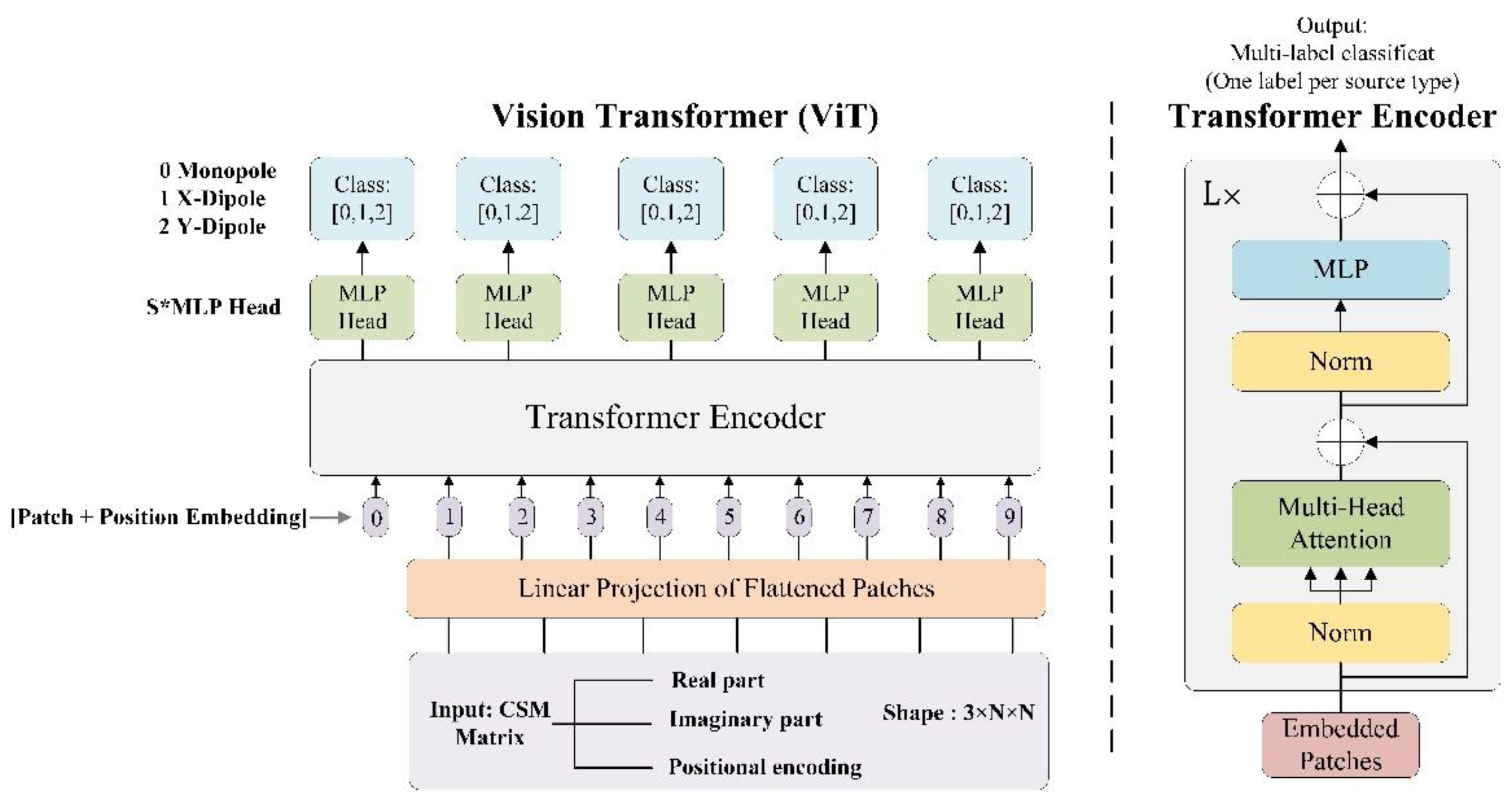
The input size of the model is . ViT first divides the input into non-overlapping image patches, each of size , resulting in patches. Each patch is linearly projected into a 768-dimensional embedding vector through a Conv2D, forming a token sequence of length 36. A learnable identification token (CLS) is prepended to the sequence, and positional embeddings are added element-wise to explicitly provide positional information. The resulting sequence of length 37 is then input into the stacked ViT encoder for feature modeling.
The ViT encoder consists of 12 identical encoder blocks. Each block contains 12 multi-head attention mechanisms and a multilayer perceptron (MLP) module. The embedding dimension is 768, and the hidden dimension of the MLP is 3072 (MLP ratio of 4). Each block uses residual connections and layer normalization. During encoding, the multi-head attention mechanism effectively captures global dependencies between patches and models the spatial distribution characteristics of frequency-domain interference patterns.
After feature extraction, the first token in the output sequence is used as the global representation of the entire image. This token is passed through MLP heads to predict the source types. There are s parallel identification heads in total, each corresponding to a specific source location, and outputting its type prediction. Here, ∈ {2, 5, 10}, representing the number of sources in the sample. Each identification head consists of two fully connected layers with channels 768→384→3, using GELU activation and dropout for regularization. Finally, a softmax layer outputs the source type at each location (0: monopole, 1: -direction dipole, 2: -direction dipole).
The overall architecture of the ViT and its model configuration are illustrated in Figure 1 and Table 1, respectively.

Table 1.
ViT model configuration.
| Layer no. | Layer type | Kernel number | Kernel size | Stride | Activation | Padding | Output size |
| 1 | Patch Embedding | 768 | 9×9 | 9×9 | Linear | No | 6x6×768 |
| 2 | Add CLS Token | - | - | - | - | - | (6×6+1)×768 |
| 3 | Add Positional Encoding | - | - | - | - | - | 37×768 |
| 4 | Dropout | - | - | - | - | - | 37×768 |
| 5-16 | Transformer Block x12 | 12 heads | - | - | GELU | - | 37×768 |
| 17 | Layer Norm | - | - | - | - | - | 37×768 |
| 18 | CLS token extract | - | - | - | - | - | 1×768 |
| 19-23 | MLP Classifier×S | 384→3 | Linear layers | GELU | - | S×3 |
Figure 1.
ViT architecture.
3.3. Training Details
During the model training phase, the Adam W optimizer is employed to update network weights, with an initial learning rate set to 1×10⁻⁴. A Cosine Annealing Warm Restarts (CAWR) scheduler is used to dynamically adjust the learning rate, enhancing convergence stability. The training is performed with a batch size of 64 for up to 200 epochs, and an early stopping strategy is applied on the validation set to prevent overfitting. To mitigate the impact of label uncertainty on model training, the loss function adopts label smoothing cross-entropy, which improves the model’s generalization in multi-class source identification tasks. Throughout training, the loss and accuracy curves for both the training and validation phases are recorded in real time. The model parameters corresponding to the lowest validation loss are saved for subsequent performance evaluation.
4. Simulations
To comprehensively evaluate the applicability and robustness of the proposed CSM–ViT–based source-type identification method under acoustically complex conditions, multiple simulations were designed and implemented. The simulations were conducted with fixed source counts of 2, 5, and 10. By verifying the identification performance under 2, 5, and 10 source conditions respectively, a representative subset of the source-count space is covered; integrating sub-models trained at these discrete counts allows the construction of a generalized framework capable of recognizing mixed monopole and dipole sources across arbitrary counts ranging from 2 to 10, with randomized locations and types.
4.1. Simulation Setup and Evaluation Metrics
In each case, both source types and spatial positions were randomly generated following a consistent rule: the simulation plane was divided into a 64 × 64 uniform grid. Each sample contained three possible source types: monopole, -direction dipole, and -direction dipole.
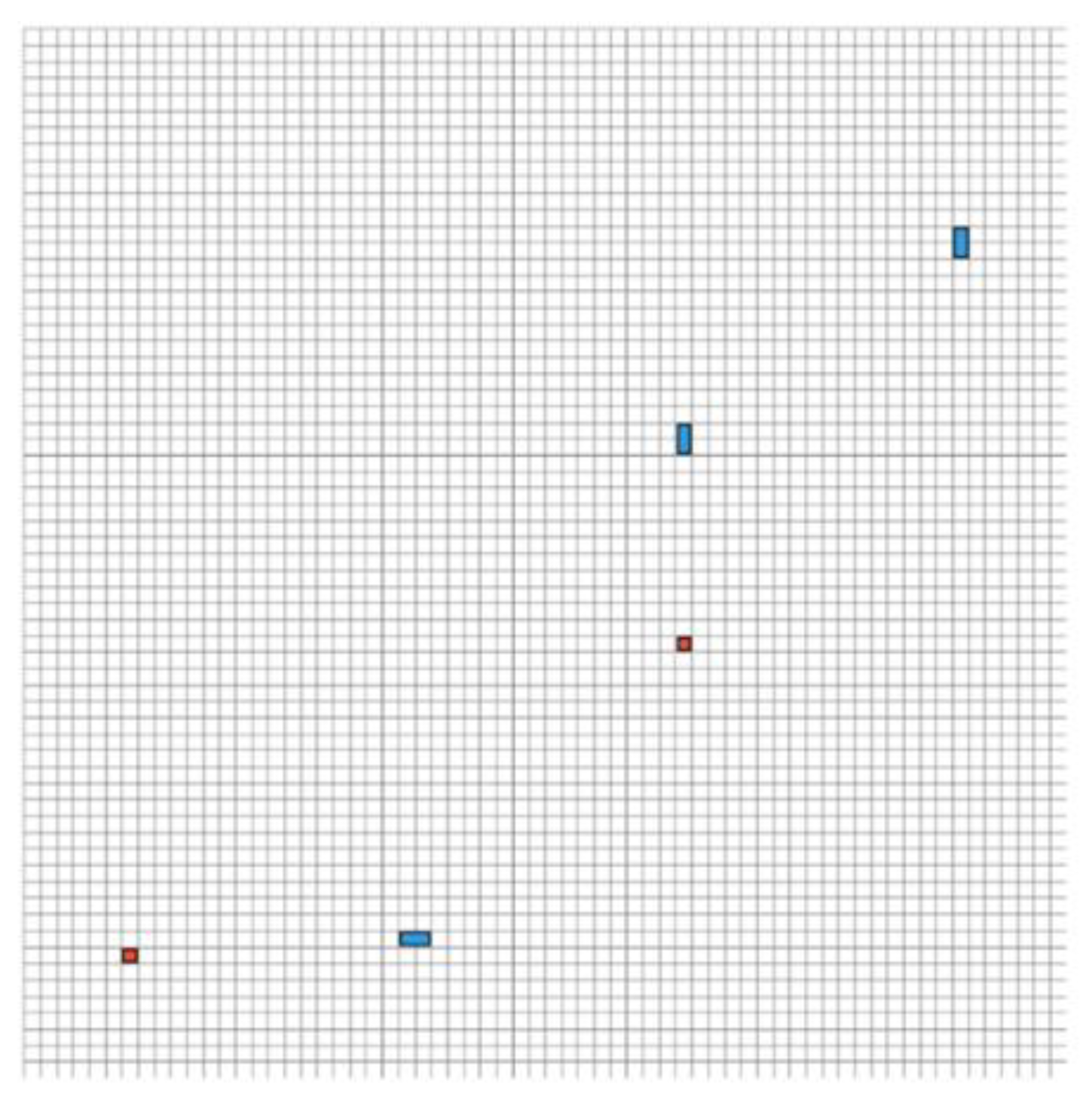
The microphone array layout is shown in Figure 2, while Figure 3 illustrates a randomized source configuration. Monopoles occupy a single red grid cell, whereas dipoles span two adjacent cells—horizontally for x-direction and vertically for y-direction dipoles—visually distinguished by blue horizontal and vertical pairs, respectively, to emphasize their directional characteristics. Each sample was guaranteed to contain at least one monopole and one dipole, with dipole types selected randomly. Overlapping of grid cells between different sources was not permitted.
Model performance was evaluated using precision, recall, F1-score, and confusion matrix metrics within a multi-label identification framework, enabling a thorough assessment of identification accuracy and generalization capability across varied complex mixtures.
Figure 2.
Microphone array layout.
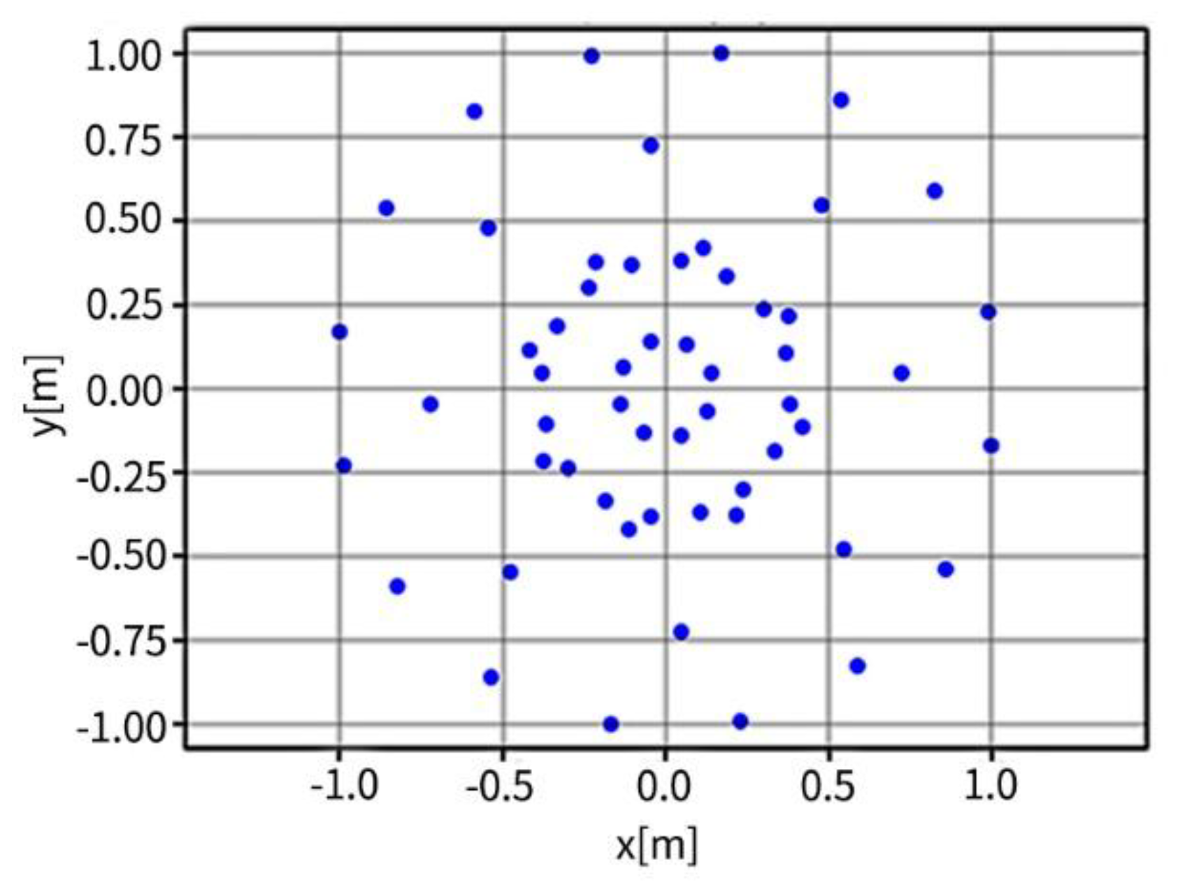
Figure 3.
Example of the randomized source layout.
The simulation cases were as follows:
Case 1: Two sources with random positions and types (monopole–dipole identification across three labels);
Case 2: Five sources with random positions and types (three-label identification);
Case 3: Ten sources with random positions and types (three-label identification).
To ensure comparability among simulations, all three cases shared consistent core parameters, as summarized in Table 2. A custom array file, Acoular_modify_array_56.xml is used, which retains the original Acoular layout but rescales the array dimensions to match the physical aperture described in the DAMAS-MS study.
Table 2.
Overview of simulation parameter settings.
| Parameter Category | Parameter Value |
| Source Frequency | 3000 Hz |
| Microphone Array | Acoular_modify_array_56.xml |
| Source-to-Array Distance | 3 m |
| Scanning Plane | 2 m × 2 m |
| Grid Spacing | 0.03125 m |
| Grid Resolution | 64 × 64 |
4.2. Simulation Analysis of Case 1
In this section, we conduct simulation under the condition of a fixed number of two sound sources. For each sample, two sources are included, with both their spatial positions and types (monopole, -direction dipole, -direction dipole) randomly generated to simulate real-world scenarios characterized by high uncertainty in source distribution and type. The corresponding ViT sub-model is trained to perform a multi-label identification task, identifying the source type at each of the two positions.
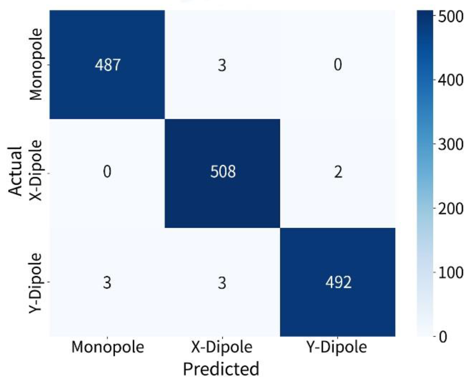
The overall confusion matrix results are shown in Figure 4 which indicates that the model achieves excellent differentiation among the three source types. The number of correctly identified monopoles, -direction dipoles, and -direction dipoles reached 487 out of 490, 508 out of 510, and 492 out of 498, respectively. The overall misidentification rate is extremely low, with minor confusion observed only between - and -direction dipoles. Notably, no systematic misidentification of monopoles as dipoles is observed.
Figure 4.
Confusion matrix for two-source identification.
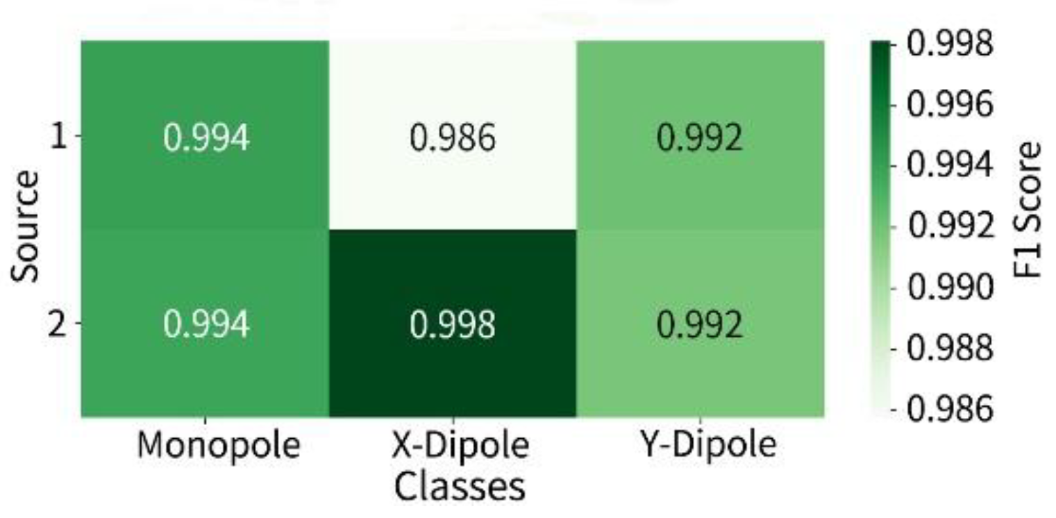
Furthermore, the identification metrics—precision, recall, and F1-score are shown in Figure 5 and Figure 6, remaining above 0.990 across all categories, with the highest F1-score reaching 0.998 for the -direction dipole, demonstrating the model’s stable and fine-grained identification capability under complex input structures. The F1-score heatmap further shows consistent performance across the two sources, with no noticeable variation due to spatial differences. Similarly, the heatmaps of precision and recall confirm that the internal attention mechanism effectively captures the structural association between source type features and spatial patterns in the CSM image.
In summary, under the condition of two-source training, the proposed ViT-based architecture exhibits strong identification accuracy for randomly located and mixed-type sources, highlighting its modeling advantages and practical value under spatial uncertainty.
4.3. Simulation Analysis of Case 2
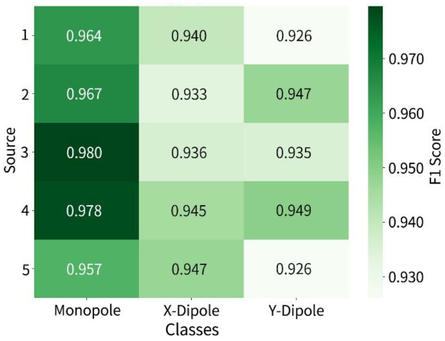
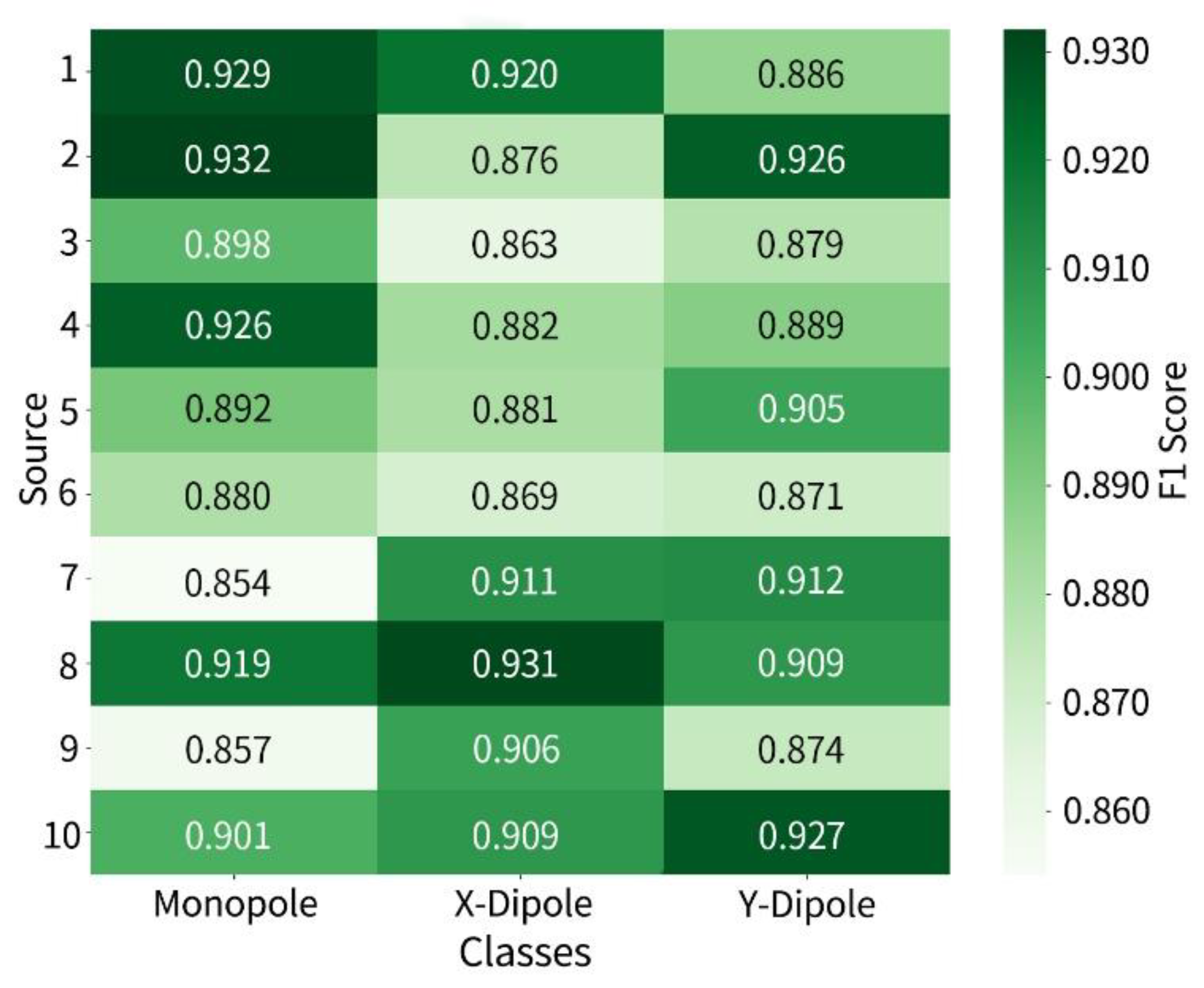
The results under the setting of five fixed sound sources are shown below. The confusion matrix is illustrated in Figure 7, the number of correctly identified sources for each class is as follows: 470 out of 485 for monopoles, 475 out of 504 for -direction dipoles, and 478 out of 511 for -direction dipoles. The overall misidentification rate remains low, though slightly higher than that observed in the two-source scenario, with a noticeable increase in mutual misidentification s between dipole types. The F1-score heatmap further is shown in Figure 8 which reveals the identification performance distribution of each source across different categories, with scores generally ranging from 0.926 to 0.980. Monopoles remain the most consistently recognized category, while the F1-scores for x- and -direction dipoles are slightly lower, primarily due to the similarity in their spatial radiation patterns.
Figure 7.
Confusion matrix for five-source identification.
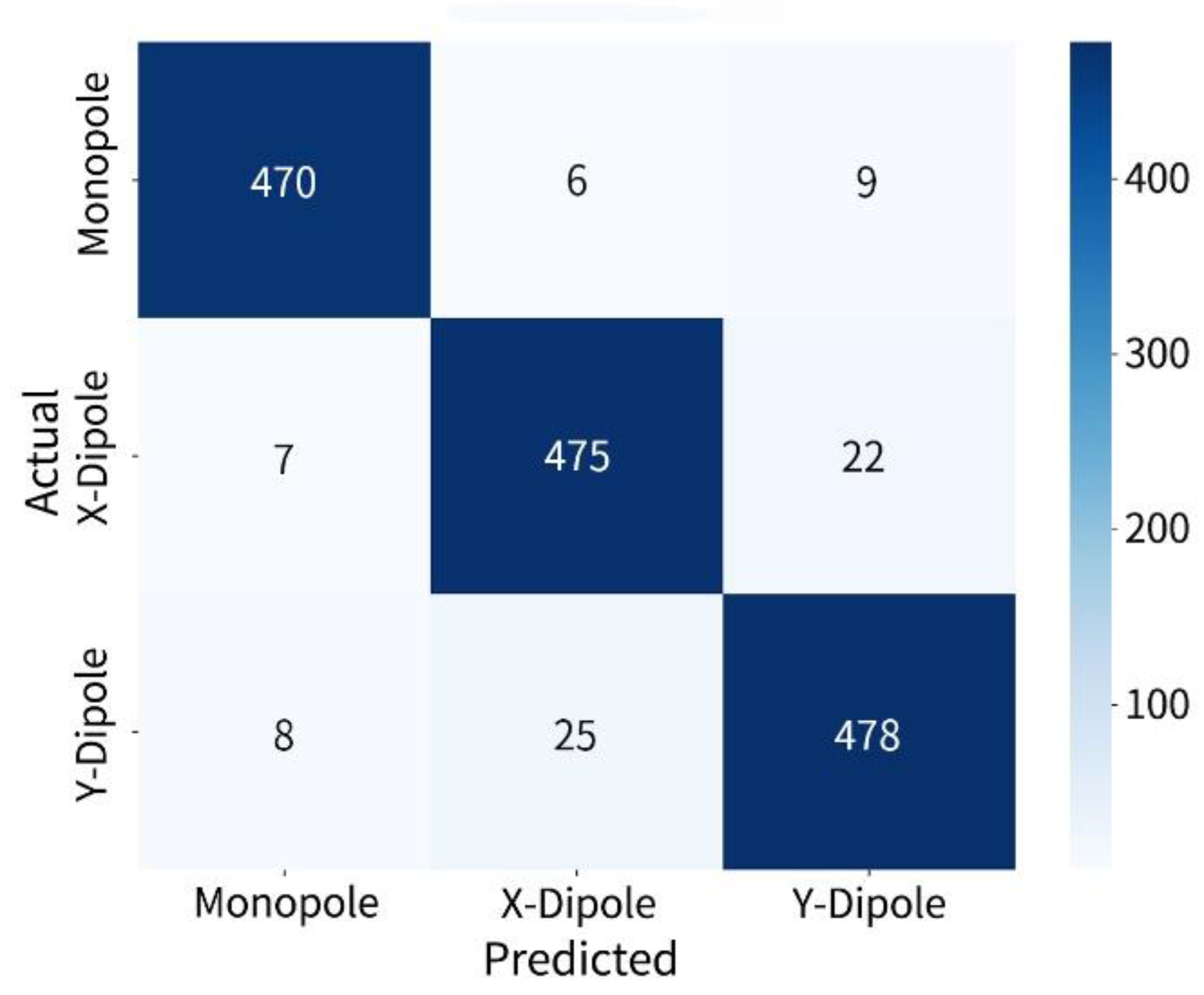
Figure 8.
F1-Score heatmap for five-source identification.
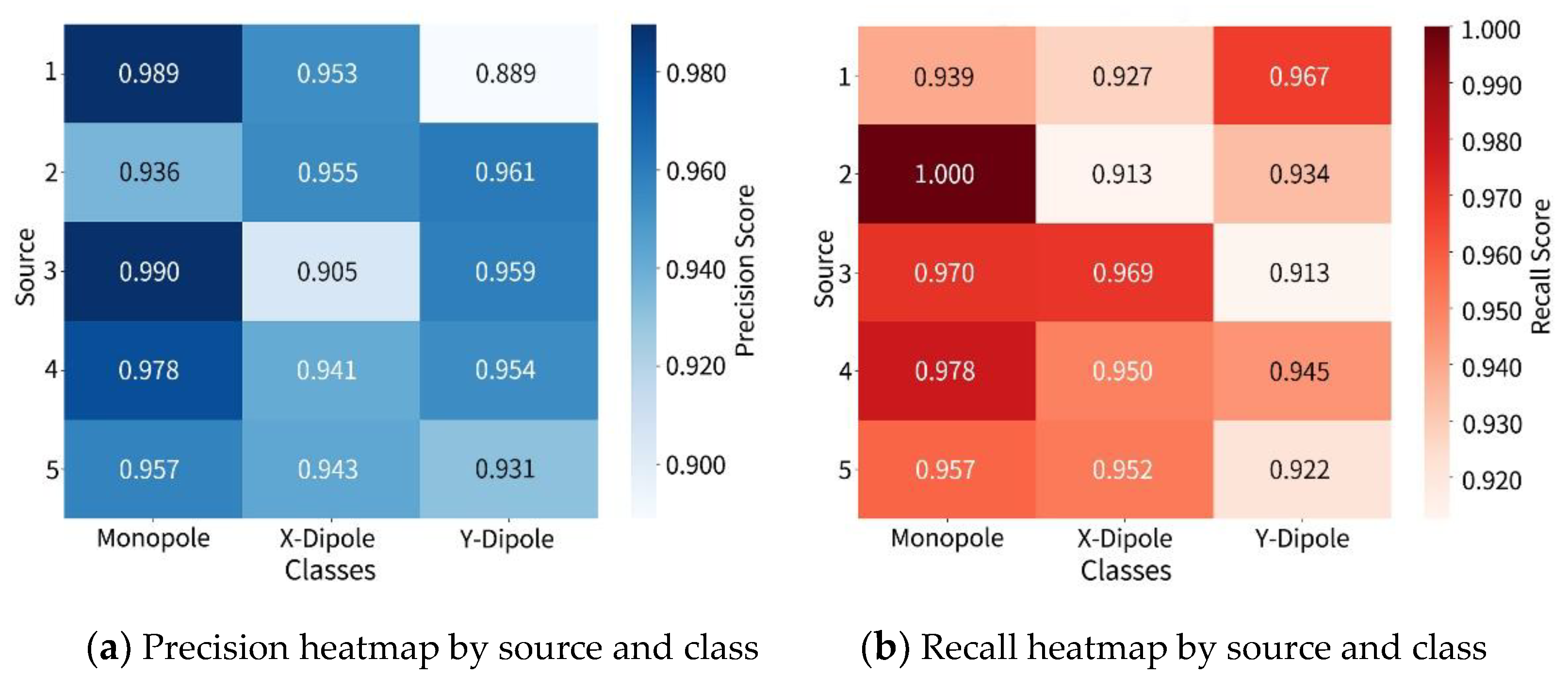
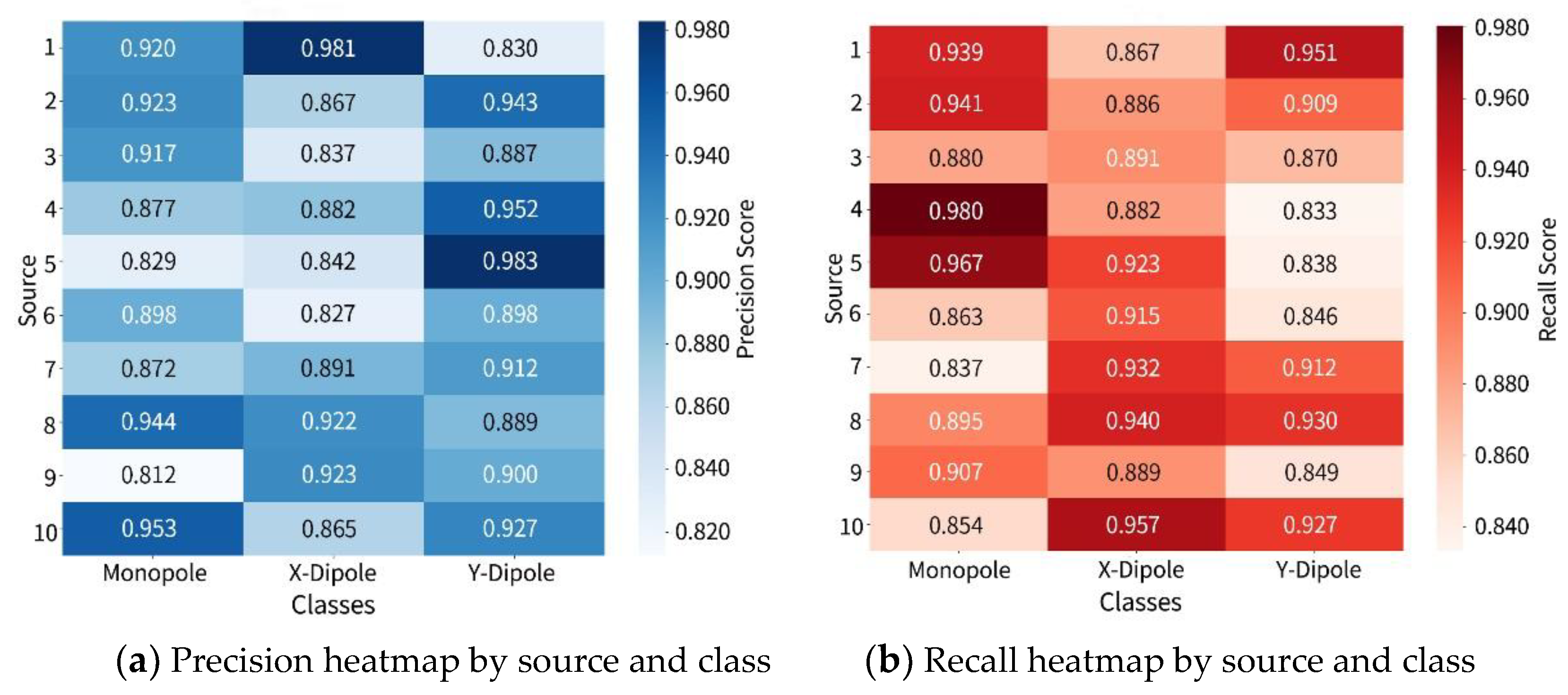
The precision and recall heatmaps are shown in Figure 9 which provide a more detailed analysis of identification performance. Some source positions exhibit a clear drop in Precision for x- and -direction dipoles (as low as 0.905). Although recall at these positions remains above 0.922, the imbalance between these two metrics suggests issues related to confidence disparities and ambiguous boundary decisions when distinguishing adjacent source types. Nevertheless, the overall performance significantly surpasses that of traditional methods and remains consistent under multi-source excitation and structural randomness, indicating that the ViT architecture possesses a certain degree of robust spatial awareness and can stably extract discriminative features from local cross-spectral patterns.
Figure 9.
Precision and recall heatmap for five-source identification.
In summary, the proposed method maintains high accuracy and strong adaptability when extended to five-source complex scenarios, demonstrating certain generalization capability and potential for practical engineering applications.
4.4. Simulation Analysis of Case 3
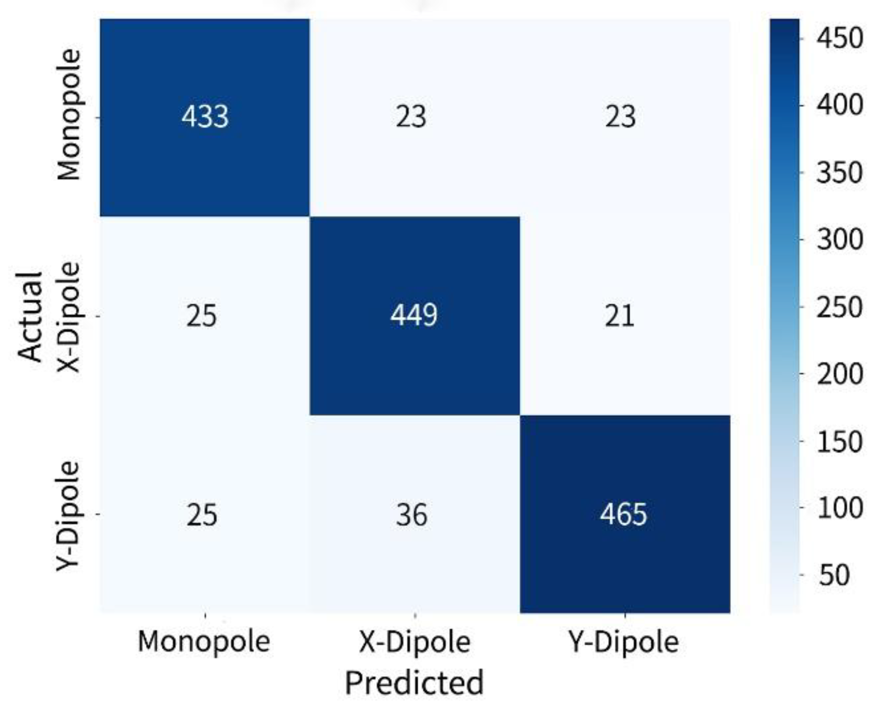
For the case with a fixed source count of ten, the confusion matrix is presented in Figure 10, showing that the model maintains a prominent diagonal dominance. The numbers of correctly identified monopoles, -direction dipoles, and -direction dipoles are 433 out of 479, 449 out of 495, and 465 out of 526, respectively. However, the misidentification rate increases compared to the previous two cases, with a certain degree of cross-type misidentification occurring between monopoles and dipoles. This indicates that under high source density, the decision boundaries between source types begin to be affected by spatial aliasing and feature ambiguity, revealing a degree of boundary generalization error in the model structure.
Figure 10.
Confusion matrix for ten-source identification.
The F1-score heatmap is shown in Figure 11 which further highlights the performance variability across source points. Compared to low-density scenarios, the F1-scores for each class are distributed in the range of 0.850–0.930, demonstrating relatively strong identification stability.
Figure 11.
F1-Score heatmap for ten-source identification.
The precision and recall heatmaps are shown in Figure 12 which exhibit more pronounced metric fluctuations. For -direction dipoles, the minimum precision is 0.827, and the minimum recall is 0.867, indicating that this category poses greater challenges for structural discrimination under complex configurations. In contrast, although monopoles also experience some misidentification, their precision and recall remain relatively stable overall, reaffirming the distinctiveness of their radiation characteristics.
Figure 12.
Precision and recall heatmap for ten-source identification.
It is noteworthy that despite a certain performance degradation, all overall indicators remain above 0.850. The model still successfully performs multi-label identification even under the extreme condition of ten highly interfering sources, demonstrating that the proposed identification framework which based on three-channel CSM construction and the ViT architecture which exhibits strong anti-interference capabilities and generalization, making it suitable for practical engineering applications in densely distributed multi-source scenarios.
4.5. Summary
The combined results from the three simulation cases with different numbers of sound sources (2, 5, and 10) demonstrate that the proposed method exhibits excellent identification performance in complex acoustic scenarios characterized by highly randomized source positions and types. Although each sub-model is trained under a fixed source count setting, all are capable of stably and accurately identifying the specific type of each source in multi-label identification tasks, with key performance metrics including precision, recall, and F1-score, consistently maintained at high levels. As the number of sources increases, slight misidentification between dipole categories is observed; however, the overall model architecture still demonstrates strong anti-interference capability and effective spatial feature decoupling.
Furthermore, compared with the results of DAMAS-MS in [15], which yields a precision of about 0.90 and a recall of approximately 0.82, the proposed method achieves significantly higher accuracy in monopole identification while maintaining the inherent advantages of DAMAS-MS in dipole identification. In the two-source case, the model exhibits near-perfect stability, with precision, recall, and F1-scores all exceeding 0.990. For the five-source case, performance remains excellent, with precision ranging from 0.905–0.980, recall above 0.922, and F1-scores between 0.926–0.980. Even under the challenging ten-source case, where slight category confusion occurs, the method maintains precision no lower than 0.827, recall above 0.867, and F1-scores between 0.850–0.930. This indicates that our method not only enhances performance where conventional methods struggle but also preserves their strengths in scenarios where they perform well.
These findings suggest that the proposed method is capable of accurately identifying arbitrary combinations of 2 to 10 mixed sources with random locations and types, thereby validating the effectiveness of representative sub-model training for generalization. The results also highlight the strong robustness and engineering applicability of the method in densely populated multi-source sound fields.
5. Experimental Verification
To assess the practical applicability and generalization of the proposed method, an acoustic experiment was conducted in an anechoic chamber. This experiment aims to extend the theoretical framework developed in simulation to engineering application scenarios, thereby assessing the method’s robustness and identification performance under real environmental conditions.
5.1. Experimental Environment and Source Configuration
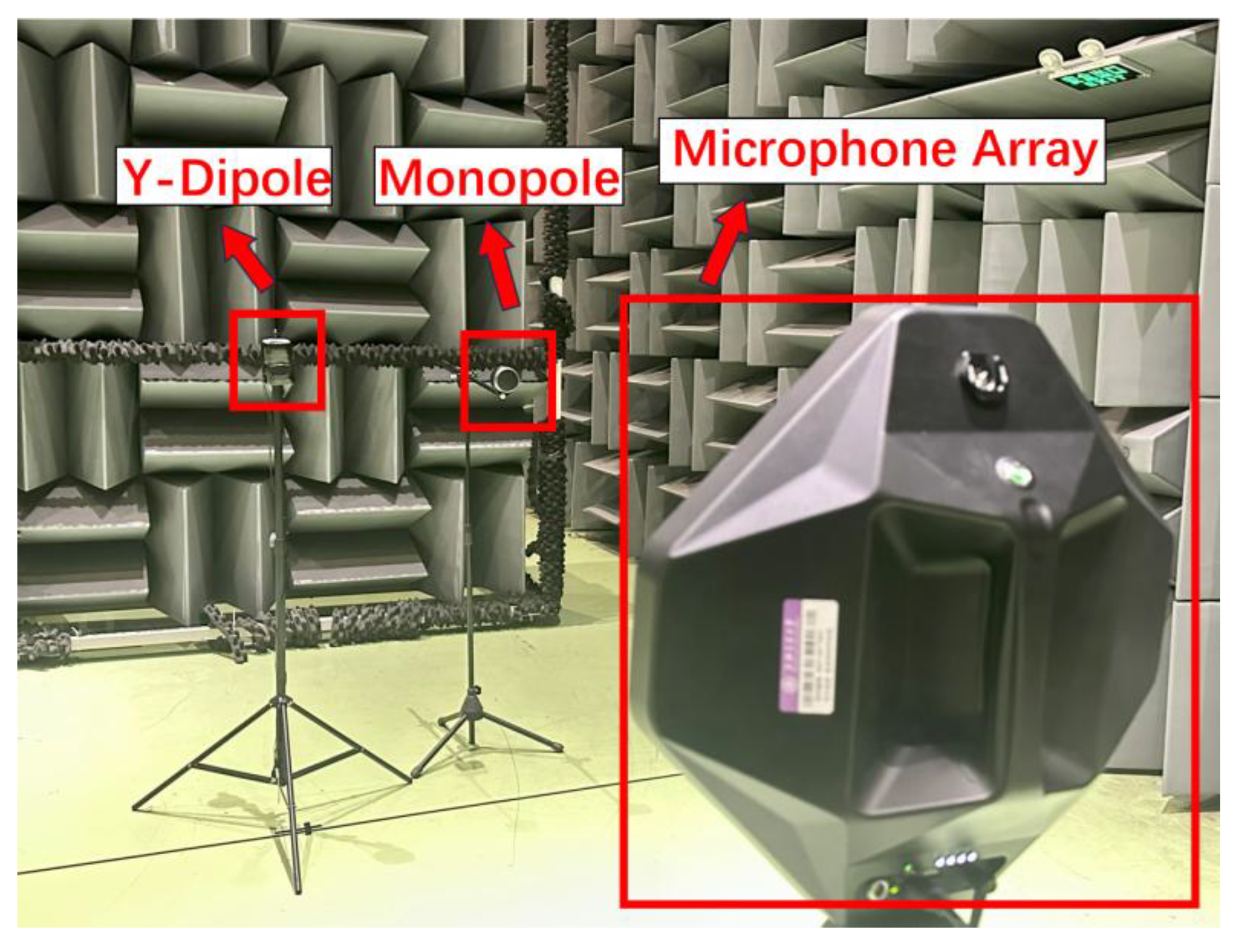
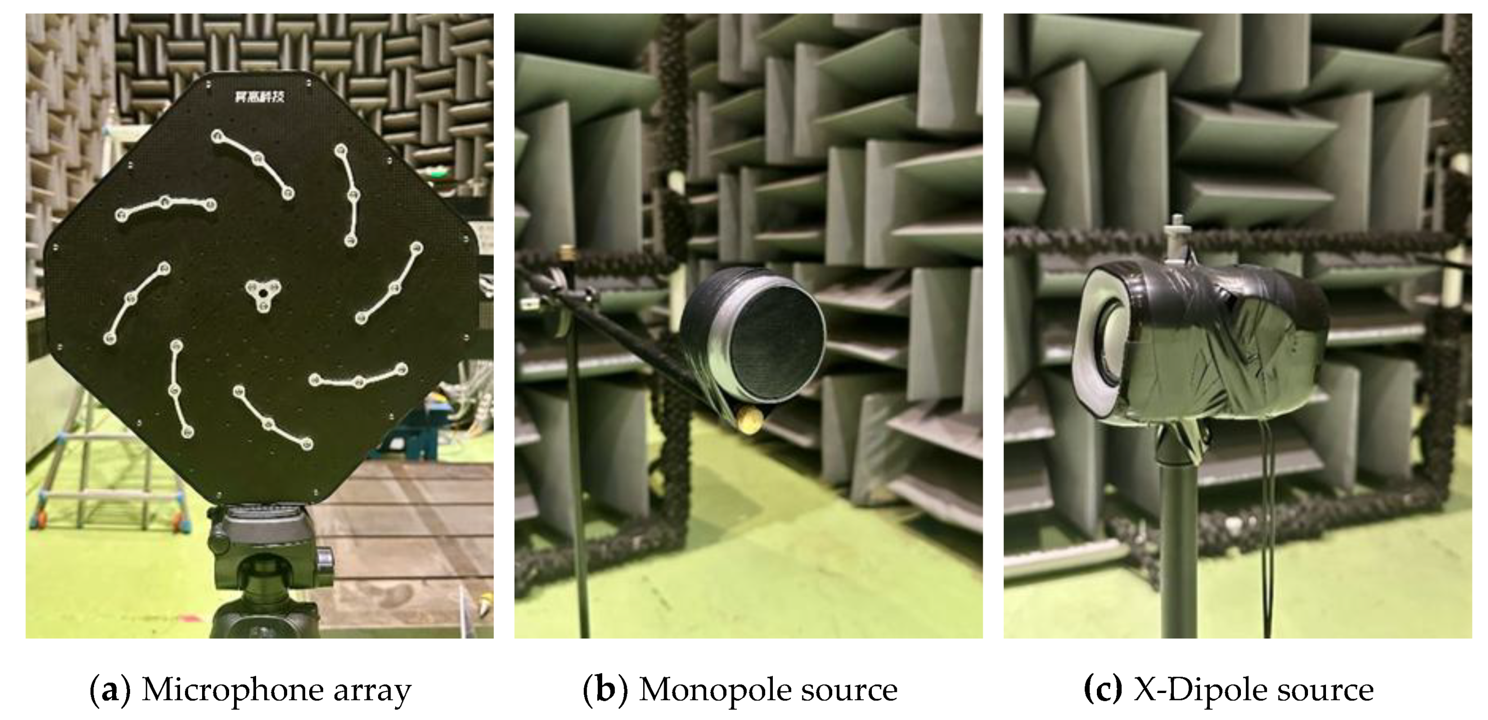
The experimental setup is shown in Figure 13. The experiment employed the DES-T144 portable high-resolution acoustic camera developed by KeyGo Technology, which integrates a 144-channel microphone array and an array imaging module. A ViT sub-model was retrained to adapt to the structure of the DES-T144 array shown in Figure 14(a) and a two-source setup with random positions and random types was selected as the core experimental scenario.
In terms of source construction, as shown in Figure 14(b), the monopole source was simulated using a single independent Bluetooth speaker (Thinkplus BT version Speaker K30), which emitted a 3000 Hz sine wave utilizing its point-like radiation characteristics. The dipole source was constructed using two identical speakers that emitted out-of-phase signals at the same frequency, thereby forming an approximately ideal dipole radiation field (see Figure 14(c)). The x-direction and -direction dipoles were implemented by placing the dual-speaker structure horizontally or vertically, respectively. All source signals were uniformly controlled via an external smartphone to ensure accurate phase alignment between the two sources and consistency with the main frequency used in the simulation.
Figure 13.
Experimental setup.
During the experiment, the distance between the sound sources and the microphone array was fixed at 3m. By manually changing the positions of the sources to simulate random locations, 20 sets of test samples were constructed with different combinations of monopoles and dipoles in various directions to simulate random types. Each group of experiments was conducted under independent conditions for data acquisition and frequency-domain processing, and the processed data were fed into the trained ViT model for identification.
Figure 14.
Experimental equipment.
5.2. Experimental Results and Analysis
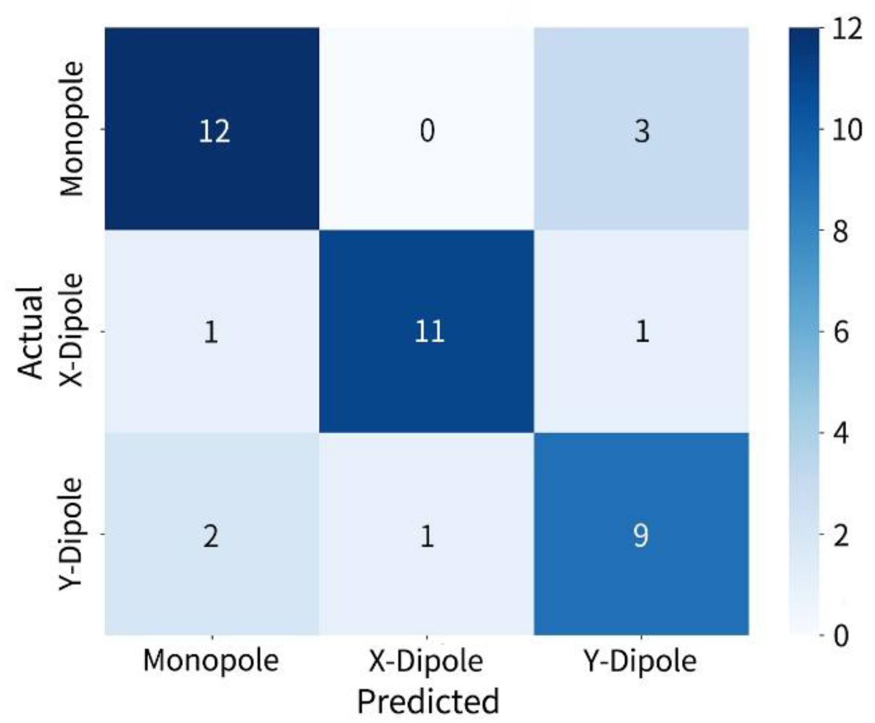
The experimental results are shown in the Figure 15. The overall confusion matrix demonstrates that the model has strong identification ability for the three types of sources. The monopole was correctly identified in 12 out of 15 cases, with most misidentifications occurring as -direction dipoles. The -direction dipole was correctly recognized in 11 out of 13 cases, with only minor misjudgments. The -direction dipole was correctly identification in 9 out of 12 cases, with some misidentification s as monopoles or -direction dipoles. Overall, the model exhibits good discriminative performance under real acoustic conditions, and the slight confusion between dipole types is mainly attributed to their similarity in radiation direction.
Figure 15.
Confusion matrix for anechoic chamber experiment.
6. Conclusions
This paper proposes a novel sound-source type identification framework that integrates beamforming-derived CSM and a ViT identifier, aiming to address the challenge of identifying monopole and dipole sources under unknown source type, position, and number. To the best of our knowledge, this is the first study that systematically applies ViT-based deep learning to multipole acoustic source identification using CSM inputs.
Simulations with fixed source counts (2,5,10) and randomized locations and types demonstrate consistently high identification accuracy across a wide range of configurations. Experimental verification in an anechoic chamber with physical monopole and dipole realizations further confirms the robustness of the model.
By combining sub-models trained on different source counts, the approach can generalize to arbitrary 2-10 source configurations. Even under limited microphone number, ViT can capture spatial phase and pressure correlations within CSM. Its robustness to local disturbances and input order makes it effective for recognizing source types and positions in highly randomized acoustic fields. The model outperforms the DAMAS-MS baseline in monopole identification accuracy. Importantly, it bypasses the ill-posedness of traditional inverse problems by learning directly from CSM, offering a practical and scalable solution for complex acoustic environments.
Funding
This work is supported by the National Natural Science Foundation of China (W2442003). The authors gratefully acknowledge the NSFC’s support in advancing acoustic measurement techniques.
References
- Crighton, D.G. “Airframe noise.” In Aeroacoustics of Flight Vehicles: Theory and Practice; Volume 1; pp. 391–447, 1991.
- Merino Martínez, R.; Sijtsma, P.; Snellen, M.; et al. “A review of acoustic imaging methods using phased microphone arrays: Part of the ‘Aircraft Noise Generation and Assessment’ Special Issue.” CEAS Aeronaut. J. 2019, 10(1), 197–230.
- Good, M.D.; Gilkey, R.H. “Sound localization in noise: the effect of signal-to-noise ratio.” J. Acoust. Soc. Am. 1996, 99(2), 1108–1117.
- Russell, D.A.; Titlow, J.P.; Bemmen, Y.-J. “Acoustic monopoles, dipoles, and quadrupoles: an experiment revisited.” Am. J. Phys. 1999, 67(8), 660–664.
- Zhang, Y.; Liu, Y. “Fast Evaluations of Integrals in the Ffowcs Williams–Hawkings Formulation in Aeroacoustics via the Fast Multipole Method.” Acoustics 2023, 5(3), 817–844.
- Sijtsma, P. “Acoustic beamforming for the ranking of aircraft noise.” In Accurate and Efficient Aeroacoustic Prediction Approaches for Airframe Noise, VKI Lecture Series 2013-03; Schram, C., Dénos, R., Lecomte, E., Eds.; von Karman Institute: Rhode-St-Genèse, Belgium, 25–29 March 2013.
- Bouchard, C.; Havelock, D.I.; Bouchard, M. “Beamforming with microphone arrays for directional sources.” J. Acoust. Soc. Am. 2009, 125(4), 2098–2104.
- Suzuki, T. “Identification of multipole noise sources in low Mach number jets near the peak frequency.” J. Acoust. Soc. Am. 2006, 119(6), 3649–3659.
- Chen, W.; Jiang, H.; He, W. “Dipole source based virtual three dimensional imaging for propeller noise. ” Aerosp. Sci. Technol. 2022, 124, 107562. [Google Scholar] [CrossRef]
- Liu, Y.; Dowling, A.P.; Quayle, A.R.; et al. “Beamforming correction for dipole measurement using two dimensional microphone arrays.” J. Acoust. Soc. Am. 2008, 124(1), 182–191.
- Porteous, R.; Prime, Z.; Doolan, C.J.; et al. “Three dimensional beamforming of dipolar aeroacoustic sources. ” J. Sound Vib. 2015, 355, 117–134. [Google Scholar] [CrossRef]
- Suzuki, T. “L1 generalized inverse beam-forming algorithm resolving coherent/incoherent, distributed and multipole sources.” J. Sound Vib. 2011, 330(24), 5835–5851.
- Demyanov, M.; Bychkov, O.; Faranosov, G.; et al. “Development of beamforming methods for uncorrelated dipole sources. In ” In Proceedings of the 7th Berlin Beamforming Conference, Berlin, Germany; 2018. [Google Scholar]
- Pan, X.; Wu, H.; Jiang, W. “Multipole orthogonal beamforming combined with an inverse method for coexisting multipoles with various radiation patterns. ” J. Sound Vib. 2019, 463, 114979. [Google Scholar] [CrossRef]
- Lobato, T.; Sottek, R.; Vorländer, M. “Identification of multipole sources with neural deconvolution.” In Forum Acusticum, Torino, Italy, 2023.
- Ma, W.; Liu, X. “Phased microphone array for sound source localization with deep learning.” Aerosp. Syst. 2019, 2(2), 71–81.
- Raumer, H.-G.; Ernst, D.; Spehr, C. “Compensation of Modeling Errors for the Aeroacoustic Inverse Problem with Tools from Deep Learning.” Acoustics 2022, 4(4), 834–848.
- Goudarzi, A. “Improving the analysis of aeroacoustic measurements through machine learning.”. Ph.D. Thesis, Universität Göttingen, Göttingen, Germany, 2023. [Google Scholar]
- Tung, A.; Gerstoft, P. “Multipole Source Capture Using Multiple Dictionary Sparse Bayesian Learning.” In Proceedings of the 2024 58th Asilomar Conference on Signals, Systems, and Computers, Pacific Grove, CA, USA, 2024.
- Pan, W.; Wei, L.; Feng, D.; et al. “Multipole transfer matrix model based sparse Bayesian learning approach for sound source identification. ” Appl. Acoust. 2024, 221, 109987. [Google Scholar] [CrossRef]
- Yuan, L.; Chen, Y.; Wang, T.; et al. “Tokens-to-Token ViT: Training vision transformers from scratch on ImageNet. In ” In Proceedings of the IEEE/CVF International Conference on Computer Vision (ICCV), Montreal, QC, Canada, 11–17 October 2021; pp. 558–567. [Google Scholar]
- Yin, H.; Vahdat, A.; Alvarez, J.M.; et al. “A-vit: Adaptive tokens for efficient vision transformer. In ” In Proceedings of the IEEE/CVF Conference on Computer Vision and Pattern Recognition (CVPR), New Orleans, LA, USA, 19–24 June 2022; pp. 10809–10818. [Google Scholar]
- Jekosch, S.; Sarradj, E. “An Inverse Microphone Array Method for the Estimation of a Rotating Source Directivity.” Acoustics 2021, 3(3), 462–472.
- Haykin, S.; Justice, J.H.; Owsley, N.L.; Yen, J.L.; Kak, A.C. Array Signal Processing; Prentice-Hall: Englewood Cliffs, NJ, USA, 1984. [Google Scholar]
- Bao, F.; Nie, S.; Xue, K.; et al. “All are worth words: A ViT backbone for diffusion models. In ” In Proceedings of the IEEE/CVF Conference on Computer Vision and Pattern Recognition (CVPR), Vancouver, BC, Canada, 18–22 June 2023; pp. 22669–22679. [Google Scholar]
- Wang, A.; Chen, H.; Lin, Z.; et al. “RepViT: Revisiting mobile CNN from ViT perspective. In ” In Proceedings of the IEEE/CVF Conference on Computer Vision and Pattern Recognition (CVPR), Seattle, WA, USA, 17–21 June 2024 (under review—arXiv preprint). [Google Scholar]
- Dosovitskiy, A.; Hoffer, E.; Singh, B.; et al. “An Image is Worth 16x16 Words: Transformers for Image Recognition at Scale.” arXiv 2020, arXiv:2010.11929.
- Alzubaidi, L.; Zhang, J.; Humaidi, A.J.; et al. “Review of deep learning: concepts, CNN architectures, challenges, applications, future directions. ” J. Big Data 2021, 8, 1–74. [Google Scholar] [CrossRef] [PubMed]
- Purwono, P.; Ma’arif, A.; Rahmaniar, W.; et al. “Understanding of convolutional neural network (CNN): a review.” Int. J. Robot. Control Syst. 2022, 2(4), 739–748.
- Shi, H.; Shao, H.; Mao, W.; Wang, Z. “Trio ViT: Post Training Quantization and Acceleration for Softmax Free Efficient Vision Transformer.” IEEE Trans. Circuits Syst. I: Regul. Pap. 2025, PP(99), 1–12.
Figure 5.
Precision and recall heatmap for two-source identification.
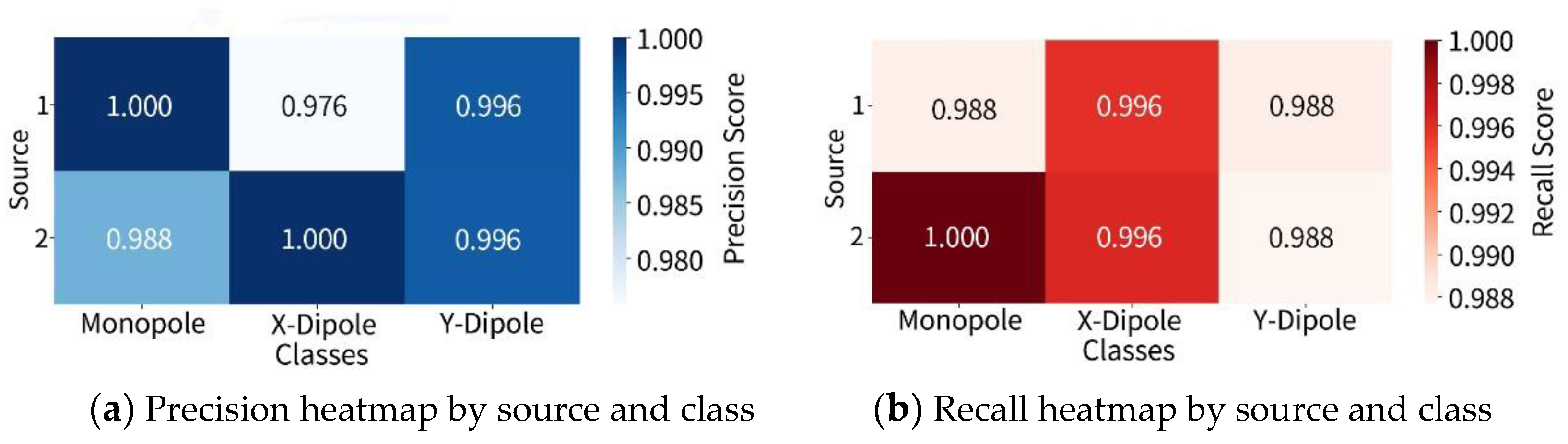
Figure 6.
F1-Score heatmap for two-source identification.
Disclaimer/Publisher’s Note: The statements, opinions and data contained in all publications are solely those of the individual author(s) and contributor(s) and not of MDPI and/or the editor(s). MDPI and/or the editor(s) disclaim responsibility for any injury to people or property resulting from any ideas, methods, instructions or products referred to in the content. |
© 2025 by the authors. Licensee MDPI, Basel, Switzerland. This article is an open access article distributed under the terms and conditions of the Creative Commons Attribution (CC BY) license (http://creativecommons.org/licenses/by/4.0/).
Copyright: This open access article is published under a Creative Commons CC BY 4.0 license, which permit the free download, distribution, and reuse, provided that the author and preprint are cited in any reuse.


