
Submitted:
19 September 2025
Posted:
22 September 2025
You are already at the latest version
Abstract
The Single Inverted Pendulum (SIP) model is widely employed in various robotics applications for balance control due to its structural simplicity and ease of implementation. Self-balancing two-wheeled transport robots offer the advantage of maintaining stability while enabling dynamic acceleration and deceleration. However, their performance is limited when carrying heavy loads, and maintaining stable balance during the loading process remains challenging. To address these limitations, this study proposes a control strategy for a pair of self-balancing two-wheeled transport robots that operate cooperatively through a separation–combination mechanism. Simulations were conducted to compare the performance of the Linear Quadratic Regulator (LQR) and Model Predictive Control (MPC) under a self-balancing condition with an external force of 100 N applied. Additionally, the proposed separation–combination method was evaluated through a simulation involving the transfer of a 20 kg delivery module. The results showed that both methods could stably transport the load, while the MPC-based approach reduced the wheel torque by approximately 50% compared to the LQR method. These findings indicate that a two-wheeled robot employing MPC in conjunction with the separation–combination method is well-suited for transporting heavy loads.
Keywords:
transport robot
; two-wheeled balancing robot
; inverted pendulum model
1. Introduction
Research on wheeled inverted pendulums (WIPs) has been conducted for many years. A basic WIP can be modeled as a single inverted pendulum (SIP) consisting of a single body mounted on two wheels. A well-known example of an SIP-based system is the Segway [1,2]. More recently, wheeled-legged robots (WLRs) such as Ascento [3] have been developed, featuring wheels mounted on articulated legs. WLRs move swiftly on flat terrain and traverse irregular terrain with the adaptability of legged robots. They also perform dynamic maneuvers including jumping and hybrid movements that combine legged walking with wheeled driving, enabling traversal of various obstacles.
WLRs equipped with manipulators have been developed for autonomous cargo handling. Handle [4] from Boston Dynamics is one such example. SIP-based robots are simple in structure, low in cost, and easy to control. However, their performance is limited when carrying heavy loads, and maintaining stable balance during the loading process remains challenging. WLRs, and WLRs with manipulators offer greater versatility yet have complex structures and require high-power actuators.
To address these limitations, this study proposes a control strategy for a pair of self-balancing, two-wheeled transport robots capable of operating either independently or as a single integrated unit through a separation–combination mechanism. Each robot can function on its own for individual tasks, yet when combined, the pair operates in perfect coordination as if it were a single, larger robot. The proposed design retains the structural simplicity of SIPs while enabling autonomous transport of heavy goods without the need for additional robotic systems or human assistance.
This approach expands the capabilities of conventional SIP-based robots to new logistics scenarios, offering a compact yet flexible solution for collaborative material transport. The remainder of this paper presents the system design, control strategy, experimental validation, and performance analysis.
2. Two-Wheeled Self-Balancing Robot
2.1. Modeling of the Two-Wheeled Self-Balancing Robot
The two-wheeled self-balancing robot is modeled as shown in Figure 1. The robot consists of the body, wheel, lift for raising transportation module, and docking mechanism. The physical specification of the robot is listed in Table 1.
Here, is the moment of inertia of the body, is the moment of inertia of the wheel, is the mass of body, is the mass of wheel, r is the radius of wheel, and l is the distance between the wheel’s COM to the body’s COM.
2.2. Dynamic Model
To obtain the robot’s dynamic model, the Lagrangian method [5,6] is used. The free-body diagram of the robot is shown in Figure 2. Here, is the reference system, and , , and are the reference systems for left wheel COM, right wheel COM, and body COM, respectively. The , , and are the robot tilt angle, wheel rotation angle, and applied torque about the wheel, respectively. Through translation and rotation, the positional vector can be obtained as shown in Equations(1)-(3).
Here, D is distance between the body COM and the wheel COM along the y-axis. The free-body diagram and the positional vector from each reference system are used to compute the robot’s kinetic and potential energy. The kinetic energy can be obtained from rotational energy or translational energy as shown in Equations (4)-(6).
Here, g is the gravitational constant. Lagrangian is defined in (7), where the potential energy is subtracted from the kinetic energy.
If the generalized coordinates are defined as , the Lagrangian equation in (7) can be computed using Equations (8)-(10).
Here, , , and are the external forces applied to the system, in which and are the left wheel torque and right wheel torque , respectively. The is the opposite of the summation of and , i.e., .
Equation (11) summarizes the solved Lagrangian Equation.
Where,
Here, M, C, G, and W are the inertia, centrifugal and Coriolis, gravity, and input matrices, respectively. The u is defined as .
The above-written equation linearized at is shown in Equation (12).
Where,
Here,
3. Plan for Self-Balancing Control
3.1. LQR (Linear Quadratic Regulator)
An LQR [8,9,10] controller is an optimal control method that computes an optimal control gain by using the state variable weight Q and the control input weight R. Here, the computed control gains are values solved from the Riccati equation and depend on the values of Q and R, which affect the system response.
3.2. MPC (Model Predictive Control)
The MPC [11,12,13] method predicts the future states until the predictive horizon using a future control input method for every data sample, enabling MPC to exhibit superior control performance. Furthermore, MPC allows for multi-input multi-output (MIMO) system that can easily adapt and consider various constraints, making it optimal for robotics control.
4. Simulation of Self-Balancing Control
The simulation environment of the two-wheeled self-balancing robot is established using a Gazebo [14,15] platform and Linux ubuntu OS 20.04, ROS1 noetic. The virtual robot is set up to be controlled using joystick, and the environment is configured to remove slip between the wheel and the road surface. To control the torque of the robot wheels, the effort controller from Gazebo is used. In addition, the JointState and IMU nodes from Gazebo are used to measure the robot’s tilt angle, body acceleration, and wheel acceleration to use them as feedback of the controllers.
4.1. Simulation of Self-Balancing Control Using LQR
Between the wheel position and the speed states, the LQR controller only used the wheel speed values as feedback. Because the chance of excessive response of the motor control and position feedback is higher owing to the non-minimum phase characteristics of the inverted pendulum system, a speed controller is safer. To verify the performance of the self-balancing control system, a 100 N of external force was exerted on the robot. The robot’s tilt angle and input torque under the external force is shown in Figure 3.
The results of the self-balancing control using LQR on a system with 100 N of external force show that the robot becomes stable within 2 s and 15° tilt angle. About -17 of input torque is needed. A demonstration video is available at Video S1 in the Supplementary Materials.
4.2. Simulation of Self-Balancing Control Using MPC
The MPC controller, like the LQR controller, only uses wheel speed for feedback. The following conditions are defined to minimize the non-minimum phase movement because of the wheel torque input, making the system more optimal for docking and undocking of the transportation module for robots:
To test the performance of self-balancing control, a 100N of external force was applied, similar to the LQR controller scenario. The robot’s tilt angle, acceleration, and input torque under the external force are shown in Figure 4.
After applying 100 N of external force on a self-balancing system using MPC, the results show that, like the LQR controller, the robot becomes stable within 2s, and about -17 of torque is needed. However, owing to the pre-configured conditions of the tilt angle, the robot stabilized within ±5° tilt angle. A demonstration video is available at Video S2 in the Supplementary Materials.
5. Simulation of Separation-Combination and Transportation
A self-balancing simulation was conducted for the transportation of goods. The simulation was conducted using transportation modules weighing 20. The simulation procedure is shown in Figure 5. After the transportation simulation was started, the robots moved towards the transportation module using the self-balancing controller. The lift was then docked, and the robots were combined using the docker located at the end of the lift. After combining, the transportation module was lifted using the lift and was moved to the desired location. After the transportation was complete, the module was lowered, lock was released, and robots were moved away after undocking. Before combining the robots or after separation, the independent movements of the robots were controlled using either the balancing controller. After combining the robots, the robots were controlled using the joystick input, and the LQR or MPC control was removed. This was because, if the transportation module was lifted from both sides, a load was introduced into the lift, causing the robot to tilt. If the robot was tilted while the LQR or MPC control was being used, the wheel torque for keeping the robot balanced became large, and the controller diverged because of the rapidly increased torque from the robot’s control goal of keeping the system upright. Furthermore, after combining, the system became statically stable owing to the four wheels, so the self-balancing controller was not needed. Thus, the balancing controllers were only used when the robots were separated.
Figure 6 is the control diagram of separation-combination and transportation. Where is the angular velocity of the left wheel, is the angular velocity of the right wheel, is the angular velocity of the left wheel, is the reference angular velocity of the right wheel, is the control torque of the left wheel, is the control torque of the right wheel, is the control torque difference of the left wheel, is the control torque difference of the right wheel, is the tilt angular velocity of the robot, is the position of the locker, and is the position of the lift. A demonstration video is available at Video S3 in the Supplementary Materials.
5.1. Simulation of the Cargo Module Using LQR
The simulation results of the LQR-based robot with 20 kg of cargo are shown in Figure 7. The simulated maximum torque for the LQR-based robot for transporting 20 kg of cargo is shown in Table 2.
The simulation results indicate that the robot can safely transport the cargo, and the largest torque applied to the wheel is 10.395 .
5.2. Simulation of the Cargo Module Using MPC
The simulation results of the MPC-based robot for transporting 20 kg of cargo are shown in Figure 8. The simulated maximum torque for the MPC-based robot for transporting 20 kg of cargo is shown in Table 3.
The simulation results indicate that the robot system can safely transport the module, and the largest wheel torque is 5.117. Compared to the previous LQR controller, a lower wheel torque of 5.278 is needed, showing that the MPC method is approximately 50% more effective.
6. Conclusion
Simulation was used to compare the performances of LQR and MPC controllers for a two-wheeled self-balancing robot with a given external force. The LQR and MPC methods both display stable performance. The MPC method exhibits superior self-balancing abilities because additional constraints can be applied. A simulation was performed for transporting heavy cargos, and both controllers showed safe and stable control. Especially, the MPC method required only 50% of the wheel torque to achieve the same performance and robot movement as the LQR method. The constraints such as wheel speed and robot tilt angle can be applied to the MPC method, making the robot more efficient when compared to the LQR method. Thus, the separation–combination cargo transportation two-wheeled self-balancing robot benefits more using the MPC method. In future work, the performances of these separation–combination cargo transportation robots using MPC will be tested for different ranges of weights and more robots. Furthermore, a physical robot is planned to be constructed and tested.
Supplementary Materials
The following supporting videos are available online at: Video S1: Simulation of self balancing control (LQR); Video S2: Simulation of self balancing control (MPC); Video S3: Simulation of separation combination and transportation (accessed on 17 September 2025).
Author Contributions
Conceptualization, S.S. and D.C.; methodology, S.S.; software, S.S. and M.C.; validation, T.K. and S.H.; formal analysis, D.K.; investigation, D.C.; resources, S.S.; data curation, S.S. and T.K; writing—original draft preparation, S.S.; writing—review and editing, D.C.; visualization, S.S. and M.C.; supervision, D.C.; project administration, D.C.; funding acquisition, D.C. All authors have read and agreed to the published version of the manuscript.
Funding
This work was supported by the Korea Research Institute for defense Technology planning and advancement (KRIT) grant funded by the Korean government (DAPA(Defense Acquisition Program Administration)) (No. 20-107-C00-007-01(KRIT-CT-22-001), Development of Multi-Legged Robot Platform for Complex Missions, 2025).
Institutional Review Board Statement
Not applicable
Informed Consent Statement
Not applicable
Data Availability Statement
The original contributions presented in the study are included in the article, further inquiries can be directed to the corresponding author.
Conflicts of Interest
The authors declare no conflicts of interest.
Abbreviations
The following abbreviations are used in this manuscript:
| SIP | Single Inverted Pendulum |
| LQR | Linear Quadratic Regulator |
| MPC | Model Predictive Control |
| WIP | Wheeled Inverted Pendulums |
| WLR | Wheeled-Legged Robots |
| COM | Center of Mass |
| MIMO | Multi-Input Multi-Output |
References
- Nguyen, H.G.; et al. Segway robotic mobility platform. In Mobile Robots XVII; Volume 5609, pp. 207–220, 2004.
- Pinto, L.J.; et al. Development of a Segway robot for an intelligent transport system. In 2012 IEEE/SICE International Symposium on System Integration (SII); pp. 710–715, 2012.
- Klemm, V.; et al. Ascento: A two-wheeled jumping robot. In 2019 International Conference on Robotics and Automation (ICRA); pp. 7515–7521, 2019.
- IEEE Spectrum Robots. Available online: https://robotsguide.com/robots/handle (accessed on 17 September 2025).
- Zefran, M.; Bullo, F. Lagrangian Dynamics. In Robotics and Automation Handbook; Kurfess, R.T., Ed.; CRC Press: Boca Raton, FL, USA, 2005; pp. 74–89. [Google Scholar]
- Spong, M.W.; et al. Robot modeling and control. Wiley: Hoboken, NJ, USA, 2006; Volume 3, pp. 75–118.
- Williams, R.L.; Lawrence, D.A. State-Space Fundamentals. In Linear State-Space Control Systems; John Wiley & Sons, Inc.: Hoboken, NJ, USA, 2007; pp. 48–107. [Google Scholar]
- Wang, H.; et al. Design and simulation of LQR controller with the linear inverted pendulum. In 2010 International Conference on Electrical and Control Engineering; pp. 699–702, 2010.
- Kumar, E.V.; Jerome, J. Robust LQR controller design for stabilizing and trajectory tracking of inverted pendulum. Procedia Eng. 2013, 64, 169–178. [Google Scholar] [CrossRef]
- Prasad, L.B.; et al. Optimal control of nonlinear inverted pendulum system using PID controller and LQR: Performance analysis without and with disturbance input. Int. J. Autom. Comput. 2014, 11, 661–670. [Google Scholar] [CrossRef]
- Wang, L. Model Predictive Control System Design and Implementation Using MATLAB®; Springer: Berlin/Heidelberg, Germany, 2009. [Google Scholar]
- Choi, D. Model Predictive Control of Autonomous Delivery Robot with Non-minimum Phase Characteristic. Int. J. Precis. Eng. Manuf. 2020, 21, 883–894. [Google Scholar] [CrossRef]
- Kim, D.; et al. Control of a two-wheeled self-balancing robot with a sliding mechanism. J. Inst. Control Robot. Syst. 2025, 31, 37–43. [Google Scholar] [CrossRef]
- Koenig, N.; Howard, A. Design and use paradigms for Gazebo, an open-source multi-robot simulator. In 2004 IEEE/RSJ International Conference on Intelligent Robots and Systems (IROS); Volume 3, pp. 2149–2154, 2004.
- Takaya, K.; et al. Simulation environment for mobile robots testing using ROS and Gazebo. In 2016 20th International Conference on System Theory, Control and Computing (ICSTCC); pp. 96–101, 2016.
Figure 1.
Simulation model of the robot
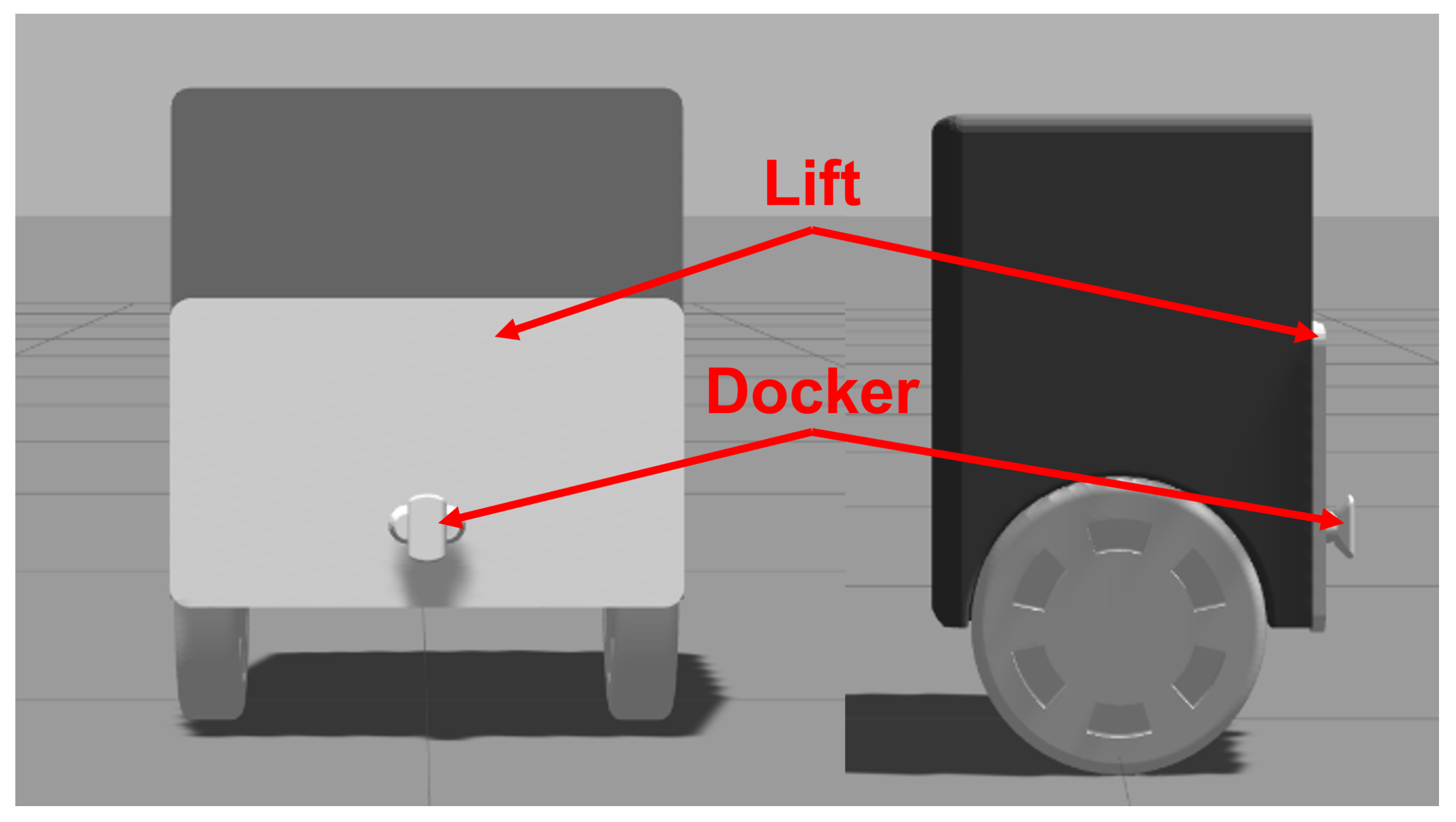
Figure 2.
Free-body diagram of the robot
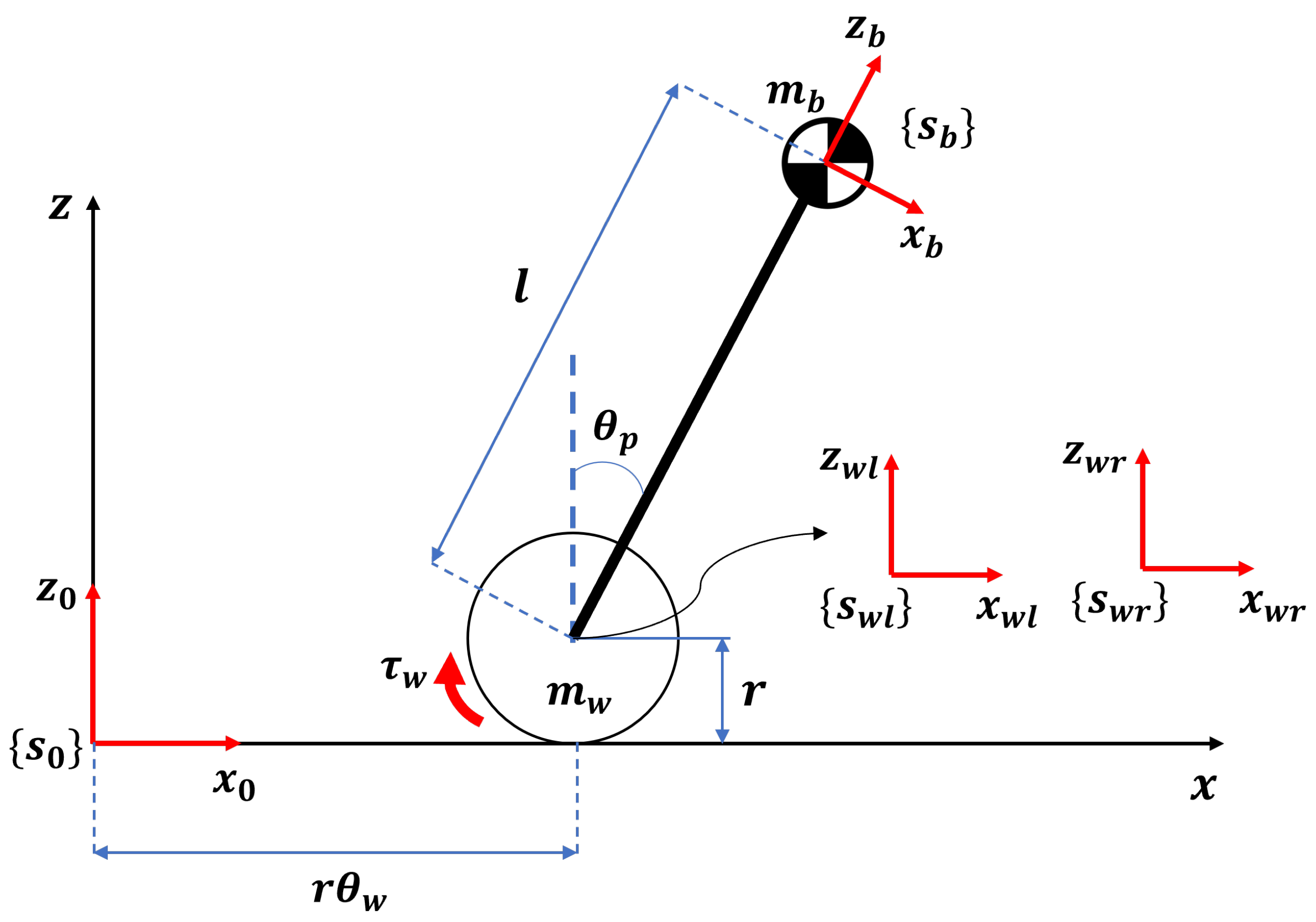
Figure 3.
Results of the LQR control
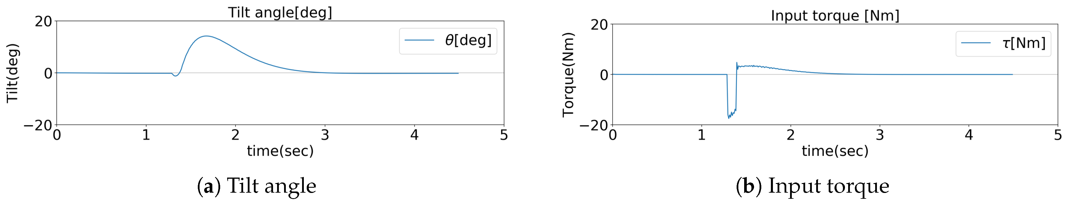
Figure 4.
Results of the MPC control
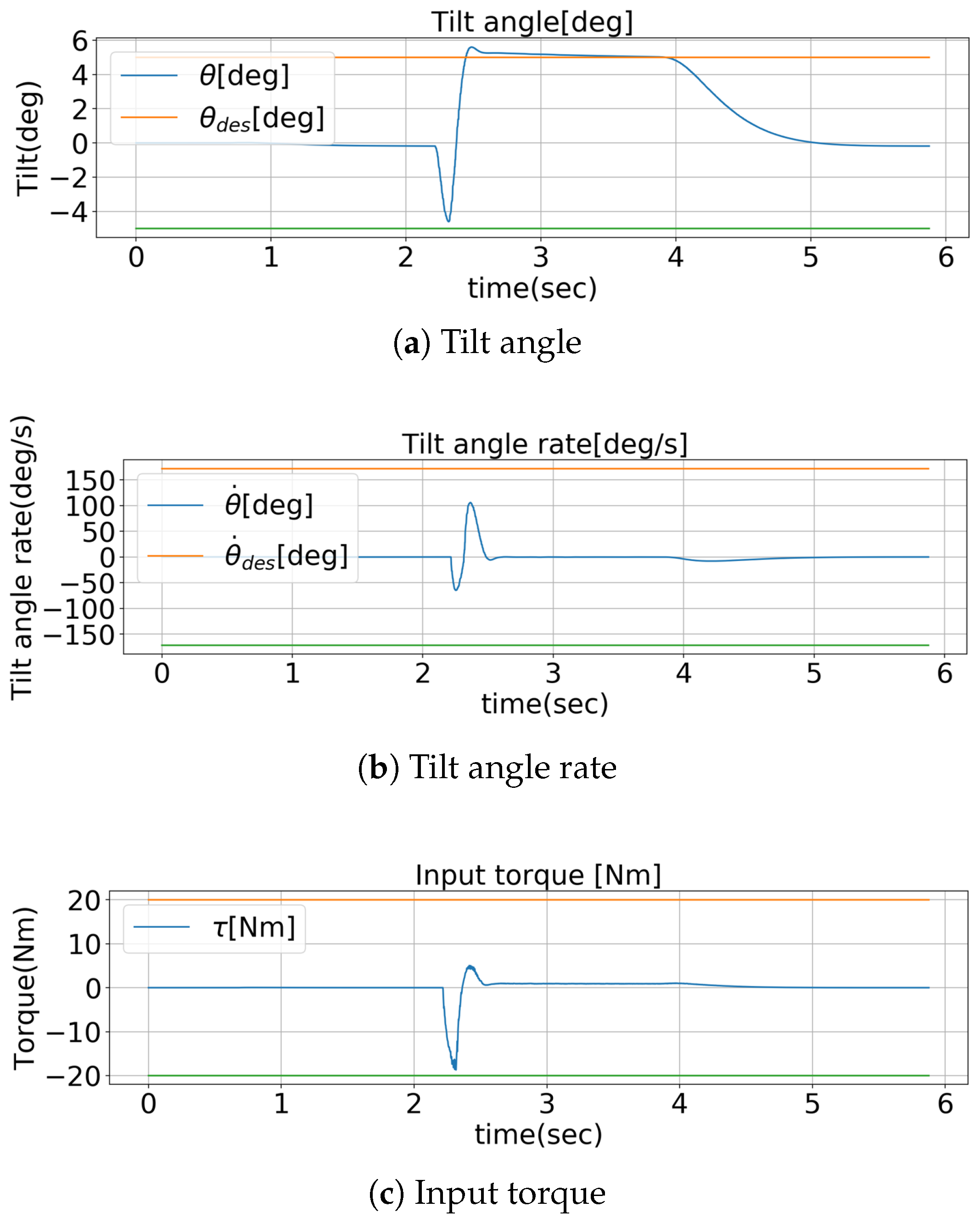
Figure 5.
Process of transport simulation
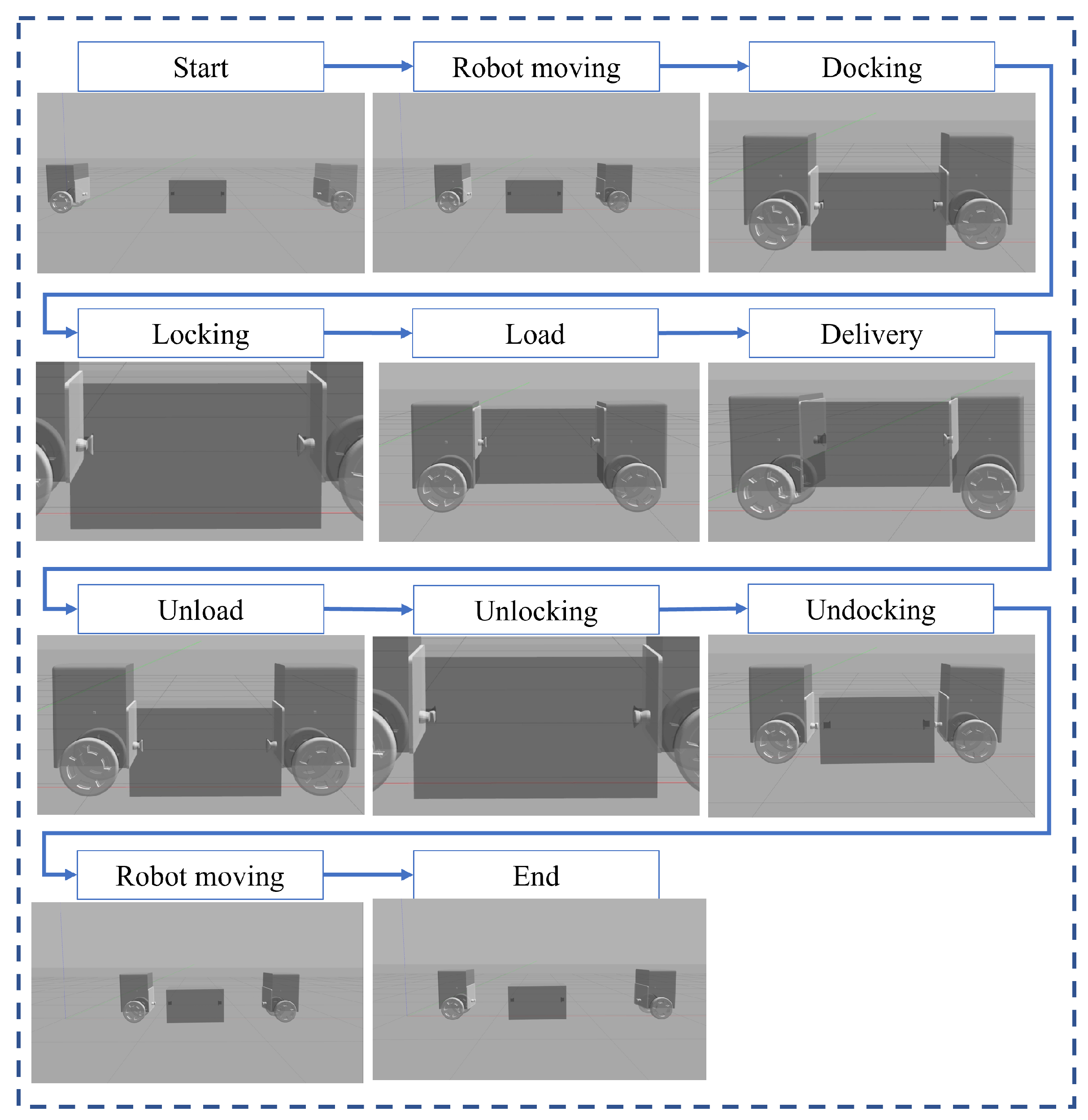
Figure 6.
Control diagram of separation-combination and transportation
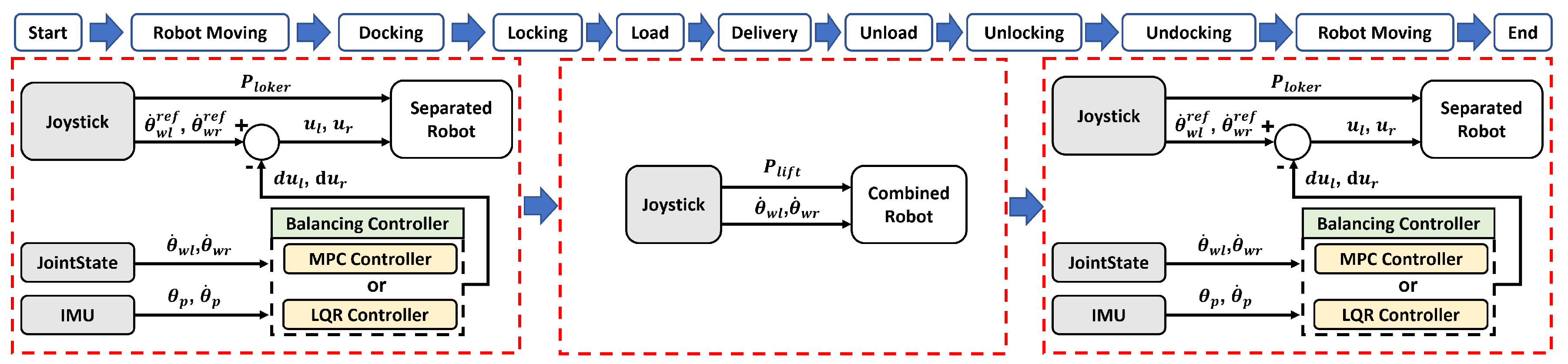
Figure 7.
Simulation results of a 20 kg module using LQR
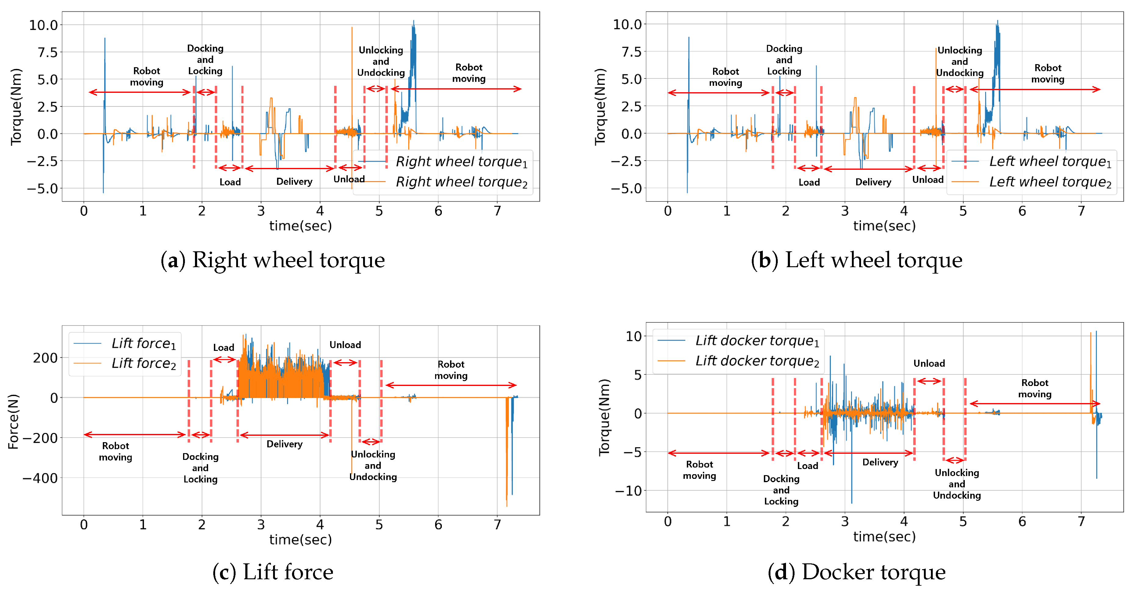
Figure 8.
Simulation results of a 20 kg module using MPC
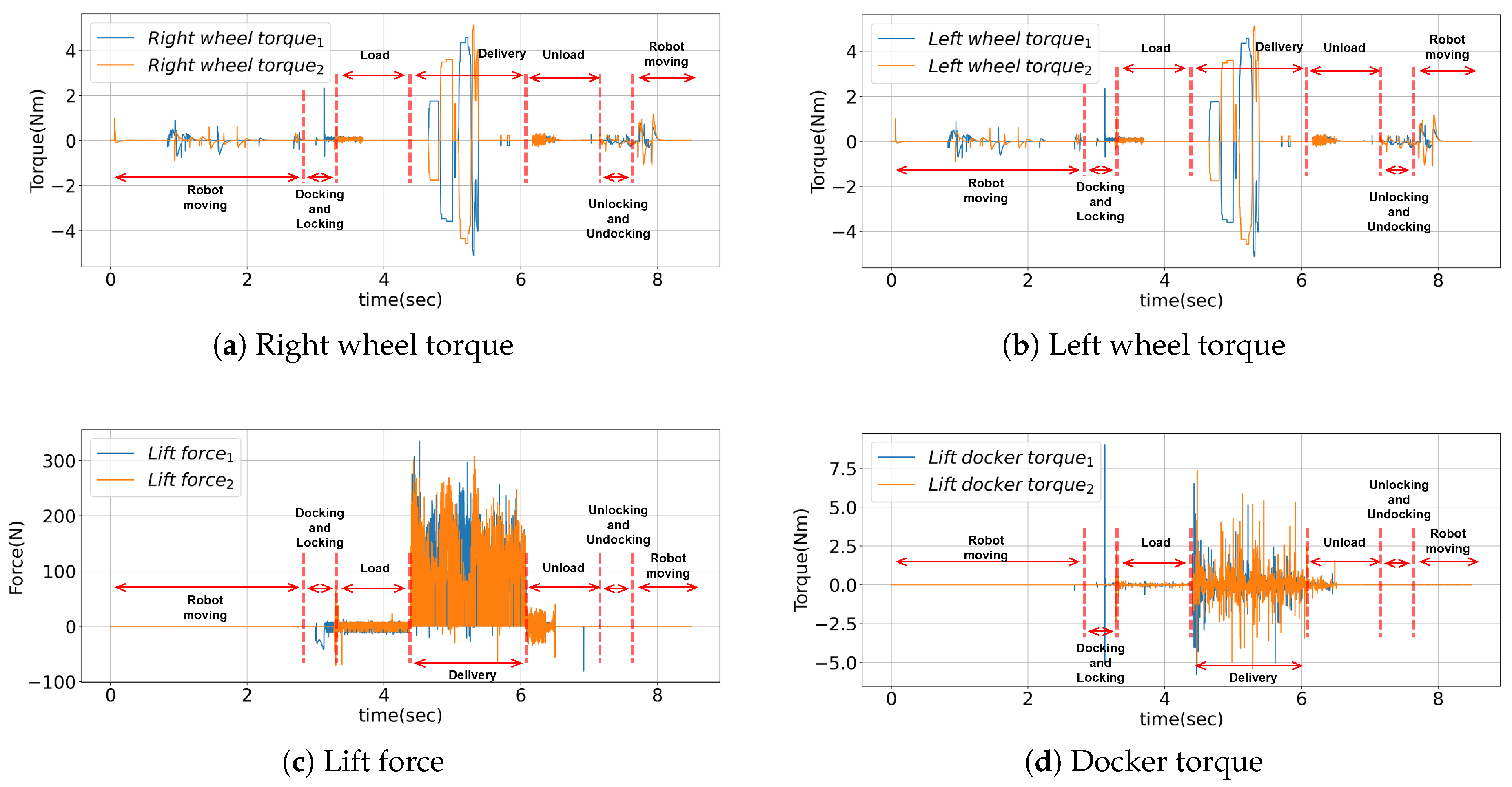

Table 1.
Specification of the two-wheeled self-balancing robot
| 0.361 | |
| 0.032 | |
| 20 | |
| 5 | |
| r | 0.115m |
| l | 0.1425m |
Table 2.
Maximum torque of a 20 kg simulation using LQR
| Robot 1 | Robot 2 | |
|---|---|---|
| Right Wheel Torque [Nm] | 10.395 | 9.771 |
| Left Wheel Torque [Nm] | 10.327 | 7.782 |
| Lift Force [N] | 317.112 | 312.477 |
| Lift Docker Torque [Nm] | 10.635 | 10.437 |
Table 3.
Maximum torque of a 20 kg simulation using MPC
| Robot 1 | Robot 2 | |
|---|---|---|
| Right Wheel Torque [Nm] | 4.574 | 5.117 |
| Left Wheel Torque [Nm] | 4.574 | 5.117 |
| Lift Force [N] | 335.328 | 307.362 |
| Lift Docker Torque [Nm] | 9.020 | 7.374 |
Disclaimer/Publisher’s Note: The statements, opinions and data contained in all publications are solely those of the individual author(s) and contributor(s) and not of MDPI and/or the editor(s). MDPI and/or the editor(s) disclaim responsibility for any injury to people or property resulting from any ideas, methods, instructions or products referred to in the content. |
© 2025 by the authors. Licensee MDPI, Basel, Switzerland. This article is an open access article distributed under the terms and conditions of the Creative Commons Attribution (CC BY) license (http://creativecommons.org/licenses/by/4.0/).
Copyright: This open access article is published under a Creative Commons CC BY 4.0 license, which permit the free download, distribution, and reuse, provided that the author and preprint are cited in any reuse.


