
Submitted:
09 June 2025
Posted:
11 June 2025
You are already at the latest version
Abstract
A modified dual hierarchical terminal sliding mode control (MDHTSMC) strategy is developed in this study for the control of a two-wheeled self-balancing robot (TWSBR). The control framework incorporates individually designed sliding surfaces within a structured dual-layer hierarchy, enabling explicit prediction of convergence time. To overcome the system’s underactuation characteristics, a hierarchical structure is embedded into the dual terminal sliding mode control law. Additionally, the proposed approach mitigates the chattering effect and enhances the system’s selfbalancing capabilities. Numerical simulations are conducted to verify the controller’s effectiveness and to confirm the theoretical results.
Keywords:
two wheeled self-balancing robot
; modified dual hierarchical terminal sliding mode control
; jellyfish search optimization algorithm
1. Introduction
The rapid development of computing, electronics, and manufacturing technologies has substantially advanced the field of mobile robotics, enabling their integration into numerous practical scenarios. These robotic systems are capable of replacing human operators in dangerous or inaccessible environments, including post-disaster rescue missions, nuclear facility maintenance, and military reconnaissance, thereby enhancing operational safety [1]. Furthermore, mobile robots play a vital role in space exploration, underwater investigation, assistive care, rehabilitation, smart transportation, and entertainment, making them increasingly indispensable in modern society [2].
The concept of the two-wheeled self-balancing robot (TWSBR) was first introduced in the late 1980s by Professor Kazuo Yamato of the Automation Department at Tokyo Telecom University, Japan, as shown in Figure 1(a). This robotic configuration presents distinct benefits when compared to conventional multi-wheeled mobile robots, including compactness and dynamic balancing capabilities, positioning it as a promising alternative in a wide range of application scenarios [3].
The TWSBR’s two wheels are arranged coaxially, enabling zero-radius turning capabilities [4]. The robot continuously maintains dynamic balance, enabling it to withstand interference and impacts that could topple statically stable robots [5]. Furthermore, its vertical orientation minimizes its spatial footprint, making it ideal for crowded and narrow indoor environments [6]. Additionally, this configuration enables the robot to function within a larger operational area, enhancing its interaction with humans [7]. These advantages have accelerated the development of TWSBRs in transportation, entertainment, and service sectors in recent years. Prominent examples include the "Segway" (Figure 1(b)) [8,9] and the "uBot" (Figure 1(c)) [10,11], among others.
Sliding Mode Control (SMC), introduced by V.I. Utkin in the 1970s, was designed to address uncertainties and disturbances and is now extensively utilized in industrial automation. The fundamental form of SMC, known as first-order Sliding Mode Control, manages simple nonlinear systems by introducing a single sliding surface, with the primary objective of guiding the system state onto this surface and maintaining sliding motion. Gao et al. study the application of SMC to a two-wheeled self-balancing robot (TWSBR), comparing it with a full state feedback controller (LQR) and demonstrating that SMC provides superior control performance for TWSBR [12]. Jmel et al. design a robust SMC for TWSBR tracking under tilt and disturbance conditions, utilizing continuous approximations near the switching surface to minimize chattering [13]. Ghahremani et al. compare the performance of cascade control with SMC for a TWSBR system [14]. Arani et al. demonstrate that SMC offers superior transient performance and noise immunity compared to LQR [15]. Sinha et al. detail the development of a robust SMC for TWSBR, where a continuous function approximates the discontinuous function, thereby achieving smoother control [16]. Yih et al. propose an SMC scheme for low-speed TWSBR speed control, demonstrating superior performance over linear optimal control in the presence of external disturbances and parameter variations [17]. Wang et al. examine the self-balancing control of TWSBR using PD and SMC, highlighting the advantages of SMC in dynamic performance, steady-state accuracy, and oscillation suppression [18]. Yang et al. present an SMC strategy that addresses matched and mismatched uncertainties in TWSBR systems by employing predefined nonlinear uncertainty bounds and reduced-order sliding mode dynamics to minimize conservatism [19]. Fukushima et al. propose an SMC method to transform a mobile robot with a wheeled arm into an inverted pendulum mode, accounting for the initial robot velocity during the transformation within a confined space. The SMC method for TWSBR is enhanced by deriving an invariant set that guarantees convergence of the system state to the origin [20]. Finally, Durdevic et al. propose a switching controller to stabilize an open-loop unstable TWSBR system with significant backlash characteristics, providing smoother performance [21].
Terminal Sliding Mode Control (TSMC), a variation of SMC, incorporates a terminal sliding surface to achieve a faster and smoother sliding motion in the control system’s terminal phase. TSMC reduces terminal-phase oscillations and instability by incorporating additional control terms into the sliding surface design, ensuring a smoother control response. Irfan et al. compare various linear and nonlinear feedback control techniques for a two-wheeled self-balancing robot (TWSBR), including LQR, SMC with feedback linearization, ISMC, and TSMC [22]. Zheng et al. propose a hierarchical fast TSMC method for TWSBR on uneven terrain, which effectively maintains balance, tracks desired speeds, suppresses disturbances, and minimizes vibrations [23].
Hierarchical Sliding Mode Control (HSMC) decomposes the control task of a complex system into multiple subtasks, with sliding mode controllers implemented at different hierarchical levels to ensure stability. Each subtask is controlled by a dedicated sliding mode controller. Hou et al. propose a method that combines HSMC with a nonlinear disturbance observer for TWSBR trajectory tracking. The system is divided into two subsystems to address coupling issues, employing an improved convergence law to control the system and suppress chattering [24]. Ping et al. propose HSMC for TWSBR, demonstrating rapid and accurate speed tracking and self-balancing performance, with robustness against partial parameter variations and external disturbances [25]. Chen et al. introduce HSMC incorporating a disturbance estimation (PE) technique for TWSBR, effectively addressing coupling effects and disturbances. The PE technique estimates system uncertainties online, thereby enhancing control performance and robustness [26].
The main contributions of this paper are as follows:
- A hierarchical sliding mode control (HSMC) scheme is combined with terminal sliding mode control (TSMC) to address the underactuated control problem of the two-wheeled self-balancing robot (TWSBR), resulting in a dual-terminal sliding mode control (DTSMC) law. Furthermore, a modified dual hierarchical terminal sliding mode control (MDHTSMC) scheme is designed based on the duality concept, with stability rigorously verified through Lyapunov theory.
- A modified dual hierarchical terminal sliding mode control (MDHTSMC) scheme is proposed for the TWSBR nonlinear system, accounting for disturbances and uncertainties. Using Lyapunov theory, finite-time convergence on the newly defined MDHTSMC surface is proven, and the arrival and sliding times are explicitly calculated.
- The Jellyfish Search Optimization (JSO) algorithm is employed to minimize the integral of the time-weighted absolute error (ITAE) by adjusting the x and parameters of the TWSBR, achieving optimal control parameters. These parameters are subsequently fine-tuned for enhanced optimization.
The remainder of the paper is structured as follows: Section 2 presents the mathematical model of the TWSBR. Section 3 introduces the DHTSMC, discusses its finite-time convergence, and provides the DHTSMC scheme with additional design parameters to derive the MHDTSMC. This section also develops the MDHTSMC design to stabilize the underactuated TWSBR system. Section 4 presents the simulation results, and finally, the conclusions are drawn in Section 5.
2. Preliminary
2.1. Dynamic Models
This section outlines the derivation of the dynamic equations governing the two-wheeled self-balancing robot (TWSBR). The dynamic model is developed based on Newtonian mechanics and vector methods, taking into account the forces and torques acting on the left and right wheels, along with the chassis, as equilibrium conditions. Figure 2 illustrates the forces and torques applied to the TWSBR, while Table 1 defines the related parameters and variables. A comprehensive derivation can be found in the literature [27,28]. The derivation here has been reorganized to enhance clarity and facilitate understanding.
Assuming no slip occurs between the wheels and the ground, the equations describing the balance of motion for the left and right wheels are expressed as follows:
Where denotes the wheel’s moment of inertia with respect to the y-axis.
The force equilibrium equations, derived from the components of the balancing forces along the x-axis and the moments about the centre of the wheel axle, are expressed as follows:
Where represents the interaction force between the pendulum and the chassis along the x-axis, and denotes the interaction moment between the pendulum and the chassis around the y-axis.
The equations for force equilibrium, derived from the forces exerted on the chassis along the x-axis and the moments about the z-axis, are formulated as follows:
Where denotes the moment of inertia of the chassis around the y-axis.
The equation derived from the equilibrium of moments acting on the chassis and pendulum about the z-axis is expressed as follows:
Where represents the moment of inertia of both the chassis and pendulum around the z-axis.
Utilizing the aforementioned five equilibrium equations, and acknowledging that , the dynamic equations for the TWSBR are formulated as follows:
where
Since
it can be concluded that is positive for all .
Furthermore, by defining and , the original system can be decomposed into two independent subsystems: rotational and longitudinal dynamics. Through the implementation of a control strategy to form a closed-loop system, sliding mode controllers (SMCs) effectively attenuate disturbances affecting the left and right wheels, denoted as and , respectively. Consequently, this approach results in a reduced-order dynamic model that facilitates the design of the TWSBR control system, as presented below:
2.2. Actuated and Underactuated Subsystems
The dynamics of the two-wheeled self-balancing robot (TWSBR) represent an underactuated system, characterized by two torque inputs controlling three degrees of freedom. Owing to the robot’s distinctive physical properties, its overall dynamics can be decoupled into two subsystems. The first subsystem, denoted as the subsystem, involves the initial dynamic equation with as its fully actuated control input. The second subsystem, referred to as the subsystem, comprises the remaining two dynamic equations, where functions as the underactuated control input.
By exploiting the robustness to parameter variations and disturbance rejection offered by variable structure control, sliding mode control (SMC) is employed to design the control inputs and . It is assumed that the reference trajectories , , and are bounded and twice continuously differentiable. Generally, these conditions are readily satisfied for and . Regarding , as previously discussed, it is influenced by the system dynamics and rolling friction. Practically, when high-order body dynamics are neglected, the conditions of boundedness and continuous differentiability for hold, enabling the achievement of the control objectives. Accordingly, the control strategy is devised to ensure that the rotational angle precisely tracks its desired trajectory while maintaining the robot body in a stable upright posture.
2.2.1. -subsystem
The -subsystem corresponds to Eq. (9) of the dynamics, which is reformulated as follows:
It is evident that this subsystem is fully actuated and can be decoupled from the remaining components of the overall system.
2.2.2. -subsystem
This subsystem is underactuated, requiring at least two variables, v and , to be controlled using only a single control input signal, . Compared to the fully actuated subsystem, controlling this underactuated subsystem is considerably more challenging and critical. Consequently, this study focuses solely on the -subsystem.
3. Modified Dual Hierarchical Terminal SMC
3.1. Dynamic Model
To begin, examine two second-order nonlinear systems, each with two inputs and two outputs, structured as follows:
where represents the system state vector; and are smooth nonlinear functions of and t; denotes the system input; is a bounded nonlinear function satisfying , where , representing uncertainties and disturbances.
3.2. Hierarchical Terminal Sliding Mode Control (HTSMC)
For the two second-order systems described in Eq. (14), two terminal sliding surfaces for TSMC are defined as follows:
where , , , and are positive design parameters. The equivalent control rate is applied to eliminate the terminal sliding dynamics on the sliding surface, ensuring and .
For the first subsystem:
For the second subsystem:
where, denotes the switching control component of the terminal sliding mode controller. For simplicity, the symbol t is generally omitted in this paper and will only appear when time dependence is explicitly involved, such as in the desired sliding mode surface , which is often abbreviated as . The second-level terminal sliding surface is then defined as:
where and are terminal sliding-mode parameters that may either be constant or vary according to different conditions. Next, the switching control law is derived following the Lyapunov stability theorem. The Lyapunov energy function is defined as:
Differentiating with respect to time t yields:
Let , where and k are positive constants.
Then:
The switching control law and the overall control law u for the control system are defined as follows:
where and .
Remark 1.
For the HTSMC system of the TWSBR, the convergence proof of the first and second sliding surfaces is fundamentally the same as the convergence process for MDHTSMC (see the proofs of Theorems 3 and 4 below); hence, a detailed analysis is not provided here, for more comprehensive information, please refer to the literature [31].
3.3. Dual Hierarchical Terminal SMC (DHTSMC)
For the system described in Eq. (14), the desired DHTSMC surface is constructed as follows:
where
where denotes the sign function, and is a positive scalar.
Two lemmas are introduced to facilitate the derivation of finite-time convergence for the DHTSM controller.
Lemma 1.
According to the work in [29], suppose the continuous function V is positive definite and fulfills the following condition:
where d is a positive constant and . Under these circumstances, the function V will reach zero starting from any initial time , and the finite convergence time can be computed as:
Lemma 2.
Consider a second-order dynamic system represented by:
The function is selected to determine the finite convergence time as discussed in [29].
where the meanings of , , and remain consistent with those in Lemma 1. By incorporating the scalar d into Eq. (27), the system dynamics are modified as follows:
with the convergence time now being:
To stabilize the second-order system depicted in Eq. (14), the DHTSM control inputs are designed according to the subsequent theorem:
Theorem 1.
DHTSM Controller Design.
The states of system (14) will reach the origin along the surface within finite time if the control inputs are defined as follows:
where for and is a positive scalar constant.
Proof.
For the system expressed in (14) and the sliding surface defined in (24), the control inputs are designed using the equivalent control approach combined with the sliding mode reaching condition, as proposed in [30]. The resulting control law is formulated as follows:
where
where, and are the equivalent control inputs ensuring and when for . The switching control inputs for , can be used to satisfy the finite-time reaching conditions of the sliding mode surface.
Consider the Lyapunov function , which results in:
Consequently, the system defined by Eq. (14) converges to the designated sliding surface given in Eq. (25), with the convergence time determined based on finite-time stability theory. Once the sliding condition is satisfied, the system dynamics reduce to the following form:
The overall convergence time can be partitioned into two distinct phases: the reaching phase and the sliding phase, depending on the relationship between the system states and the DHTSM surface. Based on Lemma 2, the total finite-time convergence duration can be estimated as follows:
where is the Lyapunov function selected for the reduced system in Eq. (36). Here, and represent the reaching time and the sliding time, respectively.
This concludes the proof.
□
Building upon Theorem 1, the parameters of the sliding surface are designed to improve the system’s performance during the reaching phase. Moreover, the modified approach provides enhanced flexibility in the controller design. Consider the system governed by Eq. (14), with the sliding surface defined as according to the following expressions:
where is a positive constant, and is a design parameter. Accordingly, the modified DHTSM control inputs are defined in the following theorem.
Theorem 2.
Modified DHTSM Controller (MDHTSMC) Design.
The second-order system described by Eq. (14) will reach the specified sliding surface , as defined in Eq. (31), within a finite time. Once on the sliding surface, the system states will converge to the origin along in finite time, provided that the control inputs are designed as follows:
where for , and is a positive scalar value. The overall finite convergence time is given by:
where is the Lyapunov function for the reduced system. Here, denotes the reaching time, and signifies the sliding time.
Proof.
The proof follows a procedure analogous to that of Theorem 1 and is therefore omitted here.
Within the MDHTSM control framework, the system’s behaviour during both the reaching and sliding phases can be enhanced by appropriately tuning the parameters and . Since the initial state is predetermined, the value of is directly influenced by , which in turn affects the distance between and . Generally, corresponds to the state at time , where holds for all . The parameter governs the reaching speed and can be adjusted to regulate the reaching time. Consequently, and jointly control the reaching phase dynamics, whereas determines the convergence rate during the sliding phase.
□
3.4. MDHTSM Controller Design for TWSBR
When the control input is set equal to in system (14), the system becomes underactuated due to having fewer control inputs than degrees of freedom. Underactuated systems are widely encountered and studied in both scientific research and engineering practice, as they enable a reduction in actuator count, leading to decreased system mass and enhanced energy efficiency. By adopting a hierarchical sliding mode framework, the proposed MDHTSM control scheme can robustly stabilise such systems [30]. The hierarchical MDHTSM controller is formulated as follows:
Theorem 3.
Consider the following underactuated nonlinear model representing the dynamics of a two-wheeled self-balancing robot (TWSBR):
where the variables satisfy the same assumptions as those outlined in system (14). The corresponding sliding mode surfaces are defined as follows:
where and are positive design parameters, and and are defined in Eq. (38). Applying the equivalent control design method yields the corresponding equivalent control inputs.
For the previously described system, the desired MDHTSM surface can be constructed as follows:
where the terms and are defined as:
where denotes the sign function, and α is a positive constant. For brevity, the time variable t is omitted throughout this paper unless explicitly required in the derivation. Accordingly, the desired sliding mode surface is abbreviated as .
Two lemmas are employed to facilitate the proof of finite-time convergence properties of the MDHTSM controller.
The equivalent control inputs and are expressed as follows:
The control law u for stabilizing the underactuated system (40) is formulated as:
This guarantees that the underactuated system described by (40) attains stability within the anticipated finite time.
Proof.
Consider the Lyapunov function candidate and take its time derivative as follows:
Define . If , then
Hence, the second-level sliding surface is stable.
Given that , selecting a sufficiently large ensures the reaching condition of the surface S. The stability proof for the sliding mode surfaces and follows the approach outlined in [31] and is therefore omitted here.
This concludes the proof.
□
It is essential to establish the asymptotic stability of the first-level sliding surfaces for various control systems.
Theorem 4.
Consider a class of underactuated systems possessing a stable equilibrium point. Define the sliding surfaces as in Eqs. (41), (42), and (43), and implement the control law given in (45). If both and its derivative are bounded, i.e., and , and the parameter η satisfies , then the first-level sliding surfaces and are guaranteed to be asymptotically stable.
Proof.
Integrating both sides of Eq. (48) yields
Then,
We can observe that
Thus, , i.e.,
From the above inequality, it follows that
This shows that , i.e.,
Given that and , we obtain from Eq. (41) that and , i.e.,
From the HSMC derivation, it is evident that the values of and do not impact system stability as long as . Consequently, the following sliding surfaces can be defined:
where and are arbitrary positive constants, with . Therefore, . Assuming that , we have:
Therefore,
From Eq. (51), we obtain
Furthermore,
Since and , we have and . If the sum of two positive terms is finite, then each must also be finite. Therefore, we have , i.e., . Hence, from Eq. (59),
Thus,
and similarly,
From Eqs. (63) and (64), it can be concluded that and (square integrable). Given that , , , and , it follows from Barbalat’s lemma that and .
In conclusion, the sliding surfaces and of the first-level subsystems are not only stable but also asymptotically stable.
□
Remark 2.
Theorem 4 applies to underactuated systems possessing a stable equilibrium point. Therefore, the boundedness conditions and are naturally fulfilled.
4. Simulation Result
The formula (13) for its subsystem is rewritten as in formula (40). The state variable is selected as , as follows:
where x represents the displacement of the TWSBR and denotes the pitch angle of the robot. The parameters of the TWSBR are as follows: , , , , , , , , .
This paper utilizes MATLAB/Simulink for simulation, employs a fixed-step solver, and sets the simulation time to 0.01 seconds. The initial condition of the system is given by the state vector , where the initial values of the state variables are , , , and . The control objective is to ensure that as , each state variable converges to 0, for .
4.1. Optimization Algorithm
The Jellyfish Search Optimization (JSO) algorithm, proposed by Saremi, Mirjalili, and colleagues in 2020, is a nature-inspired optimization method. This algorithm emulates the foraging behavior of jellyfish in the ocean, utilizing water currents and random motions to locate food sources through a cooperative group strategy. The JSO algorithm mathematically models the movement and position updates of jellyfish, enabling it to effectively solve complex optimization problems. Its main advantages include a straightforward structure, ease of implementation, and robust global optimization capabilities in high-dimensional and complex search spaces. As a result, the JSO algorithm has been extensively applied in various fields such as engineering design, parameter tuning, and path planning.
The Integral of Time-weighted Absolute Error (ITAE) criterion is widely used to assess control system performance, emphasizing the minimization of long-term error. The ITAE performance index is defined as follows:
Where denotes the error signal at time t. This criterion integrates the absolute error weighted by time, thereby assigning greater significance to errors that persist for extended durations. The typical objective in controller design is to minimise this integral, thereby improving system performance.
Given that the proposed sliding mode control method involves numerous parameters, many of which require manual tuning, an optimization algorithm is employed for parameter adjustment. The objective function is defined as
In the JSO optimization algorithm, when tuning the parameters of various sliding mode controllers, a population size of 20 and 300 iterations were selected. These values are generally determined through experimental or empirical methods to achieve an optimal balance between computational efficiency and algorithmic performance, preventing both overfitting and underfitting. The parameter bounds for the sliding mode controller within the optimization process are set to . Considering that the motor employed is a micro-reduction DC motor with a rated torque of only , and that the total torque of the two motors is , the control input is constrained within the range .
The three controllers were optimised using the JSO algorithm. The parameters of the optimised controllers, rounded to four significant figures, are as follows:
The optimized parameters of HSMC (See Appendix A.1 for details) are:
The optimized parameters of HTSMC are:
The optimized parameters of MDHTSMC are:
As shown in Figure 3, following the optimization of the three controllers (JSO-HSMC, JSO-HTSMC, and JSO-MDHTSMC), the fitness curves demonstrate the effectiveness of the JSO algorithm in terms of convergence speed and result stability. Specifically, the JSO-MDHTSMC controller exhibits the lowest fitness value, indicating superior performance on the optimization objective, whereas the JSO-HSMC and JSO-HTSMC controllers have higher fitness values, reflecting relatively lower optimization effectiveness. Overall, the JSO algorithm efficiently identifies a stable optimal solution within a high-dimensional, complex search space, particularly for the JSO-MDHTSMC controller.
Through a systematic analysis of the state response, control input, and sliding surface of the TWSBR under HSMC (Figure 4), HTSMC (Figure 5), and MDHTSMC (Figure 6), significant differences in the performance of each control strategy are evident. HSMC is capable of achieving basic system stability; however, due to the inherent chattering problem, the system exhibits significant oscillations and large control input fluctuations when dealing with uncertainty and interference, making it challenging to fully eliminate dynamic errors. In contrast, HTSMC significantly reduces the oscillation amplitude and chattering phenomenon in the control input, demonstrating higher control accuracy and robustness, thereby enabling stable system operation near the sliding surface. Nevertheless, both HSMC and HTSMC exhibit steady-state errors in the pitch angle (). MDHTSMC, on the other hand, exhibits rapid convergence and high system stability, effectively suppresses initial oscillations, and maintains the sliding surface near zero, verifying the effectiveness and robustness of the control strategy while simultaneously eliminating the steady-state error in the pitch angle (). In summary, MDHTSMC not only eliminates the steady-state error in the pitch angle () but also exhibits superior control performance, making it the most effective control strategy among the three methods.
Remark 3.
As observed in Figure 3, HSMC and HTSMC exhibit higher fitness values, primarily because the pitch angle (θ) retains a certain steady-state error in the optimization solution, resulting in a higher fitness value that cannot be minimized further. Figure 4 and Figure 5 further confirm this observation, validating our hypothesis that this issue is attributed to multiple factors, including modeling inaccuracies, external interference, and omitted friction.
4.2. Parameters Tuning
Based on the preceding analysis and figures, to achieve optimal results, we have fine-tuned the aforementioned parameters accordingly. The parameters after fine-tuning are as follows:
The optimized parameters of HSMC are:
The optimized parameters of HTSMC are:
The optimized parameters of MDHTSMC are:
To more effectively demonstrate the superiority of our proposed method, we conducted two primary simulation cases:
- the performance of each sliding mode controller under ideal, disturbance-free conditions; and
- the performance of each sliding mode controller in the presence of disturbances .
4.2.1. Case 1: Ideal State
In the absence of external interference, it is evident from Figure 7 that under HSMC, the system state and control input exhibit pronounced high-frequency oscillations. The sliding surface is slow to stabilize near the zero point, resulting in significant chattering, which may damage the actuator. From Figure 8, although HTSMC exhibits significant initial peaks, it demonstrates good overall convergence speed and stability. Once the system enters the sliding mode state, the chattering is reduced, and the sliding surface stabilizes rapidly, though the initial peak may still pose challenges in certain applications. In contrast, Figure 9 indicates that MDHTSMC offers superior control performance. The high-frequency oscillations in the system state diminish rapidly, the control input is smooth and stable, and the sliding surface quickly converges to zero and remains stable, demonstrating significant advantages in enhancing system stability.
4.2.2. Case 2: With Disturbance
Under disturbance conditions, as shown in Figure 10, the performance of HSMC remains largely unchanged compared to non-disturbance conditions, particularly in terms of chattering suppression and stability maintenance. However, this reveals its inadequate control performance under high-frequency chattering. This shortcoming underscores the advantages of alternative sliding mode control techniques, such as MDHTSMC and HTSMC, which excel in suppressing disturbances and maintaining system stability. Specifically, as shown in Figure 11, HTSMC preserves its robustness and stability under disturbances and swiftly recovers stability in complex environments, making it well-suited for applications demanding stringent disturbance suppression. However, HTSMC does show a noticeable initial peak but compensates with a commendable convergence speed and stability. MDHTSMC demonstrates strong disturbance suppression capabilities, as shown in Figure 12. Although the initial oscillation amplitude of the pitch angular velocity () slightly increases when subjected to disturbance, the system quickly stabilizes and converges to the desired state, further confirming its excellent ability to maintain system stability.
Remark 4.
Although we adjusted the system parameters, due to inaccurate mathematical modeling, neglecting frictional resistance, external disturbances, and the strong coupling inherent in the TWSBR, HSMC and HTSMC cannot ensure that all state variables of the system converge to zero, particularly the pitch angle (θ), which exhibits a small steady-state error. However, MDHTSMC can ensure that all state variables of the TWSBR are close to zero.
In summary, there are significant differences in the performance of each sliding mode controller between disturbed and undisturbed conditions. Under disturbance conditions, HSMC can achieve fundamental system stability, but the chattering issue becomes more pronounced. HTSMC demonstrates good convergence and stability under disturbance, maintaining high robustness and quickly restoring system stability, making it suitable for scenarios with strict disturbance requirements, although it exhibits a pronounced initial peak. MDHTSMC shows excellent performance under disturbance and can quickly converge to a stable state. Although the initial oscillation amplitude of the pitch angular velocity () increases under disturbance, the system rapidly stabilizes and maintains the sliding mode surface close to zero, further demonstrating its excellent ability to sustain system stability in complex environments. Therefore, MDHTSMC is significantly superior to HSMC and HTSMC in terms of disturbance rejection capability and stability.
5. Conclusions
In this paper, a MDHTSMC scheme was proposed for the TWSBR. The proposed MDHTSMC successfully integrates individual sliding surfaces through a specially designed structure, ensuring finite-time convergence of the tracking error. The underactuation challenge inherent in TWSBR was effectively addressed by implementing a hierarchical control approach within the dual terminal sliding mode framework. Moreover, the proposed control strategy demonstrated significant suppression of chattering, enhancing the stability and performance of the TWSBR during self-balancing tasks. The efficacy and efficiency of the proposed method were validated through rigorous simulation results, which confirmed the theoretical analysis and highlighted the potential of MDHTSMC for advanced control applications in underactuated robotic systems.
Author Contributions
Conceptualization, Zhang Huaqiang and Norzalilah Mohamad Nor; methodology, Zhang Huaqiang; software, Zhang Huaqiang; validation, Zhang Huaqiang, Norzalilah Mohamad Nor and Siti Nur Hanisah Umar; formal analysis, Zhang Huaqiang; investigation, Zhang Huaqiang; resources, Zhang Huaqiang; data curation, Zhang Huaqiang; writing—original draft preparation, Zhang Huaqiang; writing—review and editing, Zhang Huaqiang; visualization, Zhang Huaqiang; supervision, Norzalilah Mohamad Nor; project administration, Norzalilah Mohamad Nor; funding acquisition, not applicable. All authors have read and agreed to the published version of the manuscript.
Funding
This research received no external funding.
Institutional Review Board Statement
Not applicable.
Informed Consent Statement
Not applicable.
Data Availability Statement
The data that support the findings of this study are available from the corresponding author upon reasonable request.
Acknowledgments
The authors would like to thank the Department of Mechanical Engineering, Universiti Sains Malaysia, for providing technical support and laboratory resources during this research.
Conflicts of Interest
The authors declare no conflicts of interest.
Abbreviations
The following abbreviations are used in this manuscript:
| TWSBR | Two-Wheeled Self-Balancing Robot |
| SMC | Sliding Mode Control |
| TSMC | Terminal Sliding Mode Control |
| HSMC | Hierarchical Sliding Mode Control |
| HTSMC | Hierarchical Terminal Sliding Mode Control |
| DHTSMC | Dual Hierarchical Terminal Sliding Mode Control |
| MDHTSMC | Modified Dual Hierarchical Terminal Sliding Mode Control |
| JSO | Jellyfish Search Optimization |
| ITAE | Integral of Time-weighted Absolute Error |
| LQR | Linear Quadratic Regulator |
| PD | Proportional-Derivative |
References
- S. Zhang, J. Yao, Y. Wang, Z. Liu, Y. Xu, and Y. Zhao, “Design and motion analysis of reconfigurable wheel-legged mobile robot,” Defence Technology, vol. 18, no. 6, pp. 1023–1040, 2022. [CrossRef]
- F. Rubio, F. Valero, and C. Llopis-Albert, “A review of mobile robots: Concepts, methods, theoretical framework, and applications,” Int. J. Adv. Robot. Syst., vol. 16, no. 2, p. 01–22, 2019. [CrossRef]
- Y. Olmez, G. O. Koca, and Z. H. Akpolat, “Clonal selection algorithm based control for two-wheeled self-balancing mobile robot,” Simulation modelling practice and theory: International journal of the Federation of European Simulation Societies, no. 118, p. 118, 2022. [CrossRef]
- Y. Guo, J. Guo, L. Liu, Y. Liu, and J. Leng, “Bioinspired multimodal soft robot driven by a single dielectric elastomer actuator and two flexible electroadhesive feet,” Extreme Mech. Lett., vol. 53, p. 101720, 2022. [CrossRef]
- M. B. Khan, T. Chuthong, C. D. Do, M. Thor, P. Billeschou, J. C. Larsen, and P. Manoonpong, “icrawl: an inchworm-inspired crawling robot,” IEEE Access, vol. 8, pp. 200 655–200 668, 2020. [CrossRef]
- P. Wang, Q. Tang, T. Sun, and R. Dong, “Research on stability of the four-wheeled robot for emergency obstacle avoidance on the slope,” Recent Pat. Eng., vol. 15, no. 5, p. 15, 2021. [CrossRef]
- F. Nker, “Proportional controlled moment of gyroscope for two-wheeled self-balancing robot,” J. Vib. Control, 2021.
- D. Voth, “Segway to the future [autonomous mobile robot],” IEEE Intell. Syst., vol. 20, no. 3, pp. 5–8, 2005. [CrossRef]
- A. Delgado-Spíndola, R. Campa, E. Bugarin, and I. Soto, “Design and real-time implementation of a nonlinear regulation controller for the rmp-100 segway twip,” Mechatronics, vol. 79, pp. 102 668–, 2021. [CrossRef]
- J. Zhao, X. Cui, Y. Zhu, and S. Tang, “A new self-reconfigurable modular robotic system ubot: Multi-mode locomotion and self-reconfiguration,” in 2011 IEEE International Conference on Robotics and Automation. IEEE, 2011, pp. 1020–1025. [CrossRef]
- X. Cui, Y. Zhu, J. Zhao, S. Piao, and E. Yang, “Bio-inspired locomotion control for ubot self-reconfigurable modular robot,” in 2023 International Conference on Control, Automation and Diagnosis (ICCAD). IEEE, 2023, pp. 01–06. [CrossRef]
- D. Y. Gao, P. W. Han, D. S. Zhang, and Y. J. Lu, “Study of sliding mode control in self-balancing two-wheeled inverted car,” Appl. Mech. Mater., vol. 241, pp. 2000–2003, 2013.
- I. Jmel, H. Dimassi, S. Hadj-Said, and F. M’Sahli, “Sliding mode control for two wheeled inverted pendulum under terrain inclination and disturbances,” in 2021 9th International Conference on Systems and Control (ICSC). IEEE, 2021, pp. 467–471. [CrossRef]
- A. Ghahremani and A. K. Khalaji, “Simultaneous regulation and velocity tracking control of a two-wheeled self-balancing robot,” in 2023 International Conference on Control, Automation and Diagnosis (ICCAD). IEEE, 2023, pp. 1–6. [CrossRef]
- M. S. Arani, H. E. Orimi, W.-F. Xie, and H. Hong, “Comparison of sliding mode controller and state feedback controller having linear quadratic regulator (lqr) on a two-wheel inverted pendulum robot: Design and experiments,” 2018. [CrossRef]
- A. Sinha, P. Prasoon, P. K. Bharadwaj, and A. C. Ranasinghe, “Nonlinear autonomous control of a two-wheeled inverted pendulum mobile robot based on sliding mode,” in 2015 International Conference on Computational Intelligence and Networks. IEEE, 2015, pp. 52–57. [CrossRef]
- C.-C. Yih, “Sliding-mode velocity control of a two-wheeled self-balancing vehicle,” Asian J. Control, vol. 16, no. 6, pp. 1880–1890, 2014. [CrossRef]
- L. Wang and J. Lei, “Research on self-balancing control for upright vehicle with two wheels based on sliding mode control,” in 2017 International Conference on Computer Technology, Electronics and Communication (ICCTEC). IEEE, 2017, pp. 1192–1195. [CrossRef]
- Y. Yang, X. Yan, K. Sirlantzis, and G. Howells, “Regular form-based sliding mode control design on a two-wheeled inverted pendulum,” Int. J. Model. Identif. Control, vol. 37, no. 3/4, pp. 312–320, 2021. [CrossRef]
- H. Fukushima, K. Muro, and F. Matsuno, “Sliding-mode control for transformation to an inverted pendulum mode of a mobile robot with wheel-arms,” IEEE Trans. Ind. Electron., vol. 62, no. 7, pp. 4257–4266, 2014. [CrossRef]
- P. Durdevic and Z. Yang, “Hybrid control of a two-wheeled automatic-balancing robot with backlash feature,” in 2013 IEEE International Symposium on Safety, Security, and Rescue Robotics (SSRR). IEEE, 2013, pp. 1–6. [CrossRef]
- S. Irfan, A. Mehmood, M. T. Razzaq, and J. Iqbal, “Advanced sliding mode control techniques for inverted pendulum: Modelling and simulation,” Engineering science and technology, an international journal, vol. 21, no. 4, pp. 753–759, 2018.
- N. Zheng, Y. Zhang, Y. Guo, and X. Zhang, “Hierarchical fast terminal sliding mode control for a self-balancing two-wheeled robot on uneven terrains,” in 2017 36th Chinese Control Conference (CCC). IEEE, 2017, pp. 4762–4767. [CrossRef]
- M. Hou, X. Zhang, D. Chen, and Z. Xu, “Hierarchical sliding mode control combined with nonlinear disturbance observer for wheeled inverted pendulum robot trajectory tracking,” Appl. Sci. (Basel), vol. 13, no. 7, p. 4350, 2023. [CrossRef]
- H. Ping, W. Hai, L. Linfeng, K. Huifang, Y. Ming, J. Canghua, et al., “A novel hierarchical sliding mode control strategy for a two-wheeled self-balancing vehicle,” in 2017 36th Chinese Control Conference (CCC). IEEE, 2017, pp. 3731–3736. [CrossRef]
- L. Chen, H. Wang, Y. Huang, Z. Ping, M. Yu, X. Zheng, et al., “Robust hierarchical sliding mode control of a two-wheeled self-balancing vehicle using perturbation estimation,” Mech. Syst. Signal Process., vol. 139, p. 106584, 2020. [CrossRef]
- K. D. Do and G. Seet, “Motion control of a two-wheeled mobile vehicle with an inverted pendulum,” J. Intell. Robot. Syst., vol. 60, no. 3-4, pp. 577–605, 2010. [CrossRef]
- F. Grasser, A. D’arrigo, S. Colombi, and A. C. Rufer, “Joe: A mobile, inverted pendulum,” IEEE Trans. Ind. Electron., vol. 49, no. 1, pp. 107–114, 2002. [CrossRef]
- E. Moulay and W. Perruquetti, “Finite time stability and stabilization of a class of continuous systems,” J. Math. Anal. Appl., vol. 323, no. 2, pp. 1430–1443, 2006. [CrossRef]
- A. Levant, “Sliding order and sliding accuracy in sliding mode control,” Int. J. Control, vol. 58, no. 6, pp. 1247–1263, 1993. [CrossRef]
- W. Wang, J. Yi, D. Zhao, and D. Liu, “Design of a stable sliding-mode controller for a class of second-order underactuated systems,” IEE Proc. Contr. Theory Appl., vol. 151, no. 6, pp. 683–690, 2004. [CrossRef]
Figure 1.
Different types of TWSBR robots: (a) The concept, (b) Segway, (c) uBot.
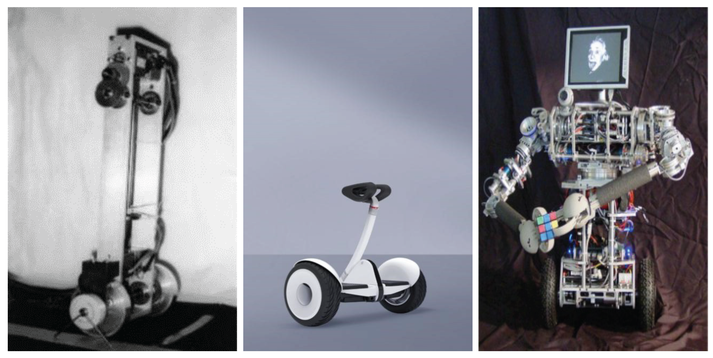
Figure 2.
Math model of TWSBR: (a) TWSBR, (b) Left wheel, (c) Right wheel.
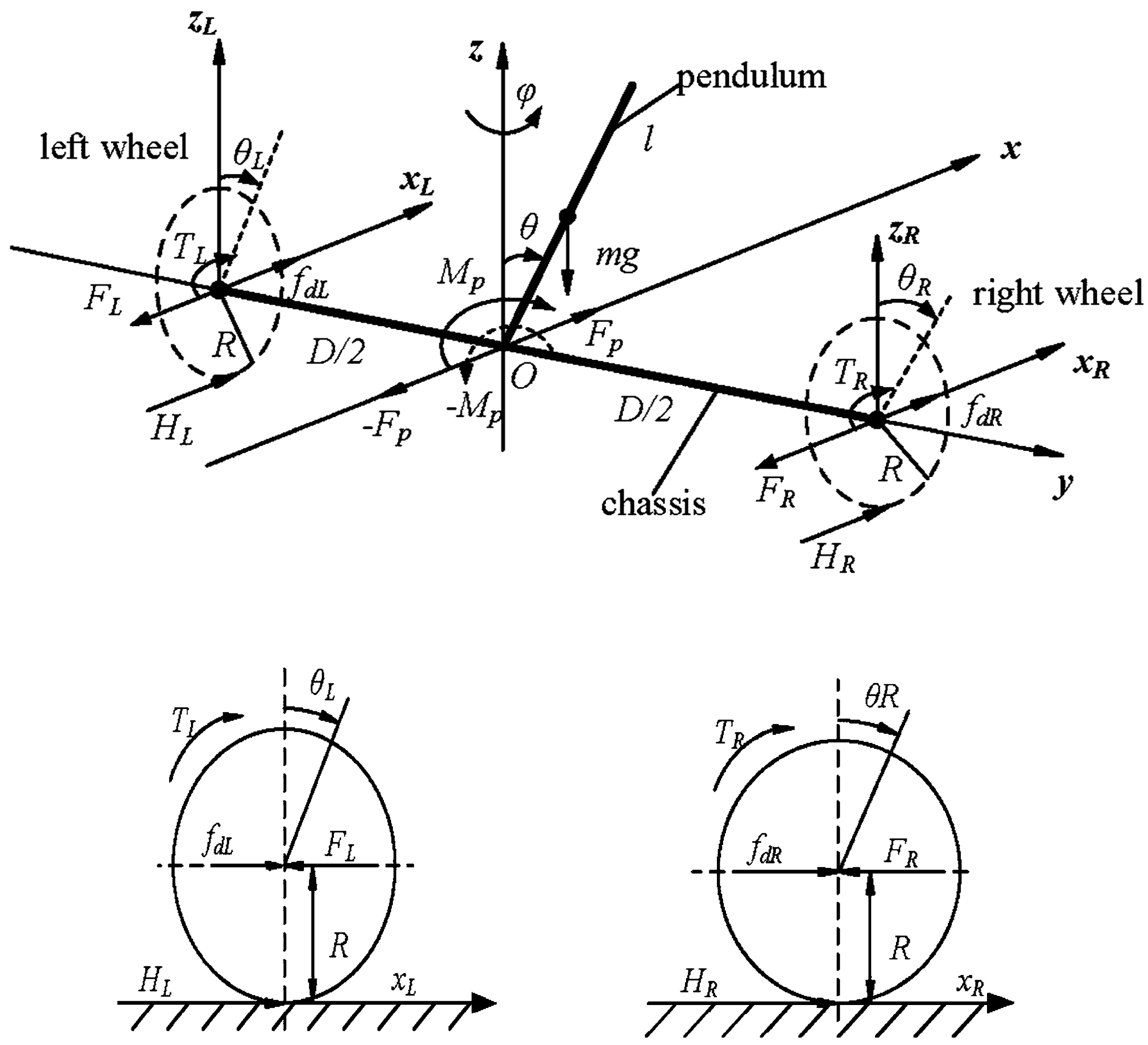
Figure 3.
Fitness graph of JSO optimization algorithm
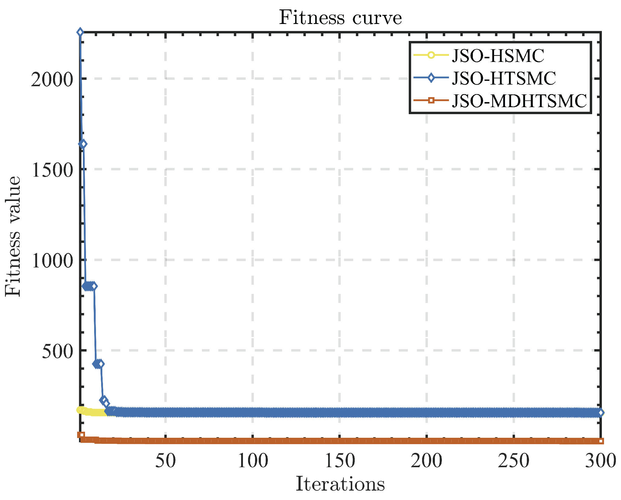
Figure 4.
Performance of HSMC under JSO optimization algorithm
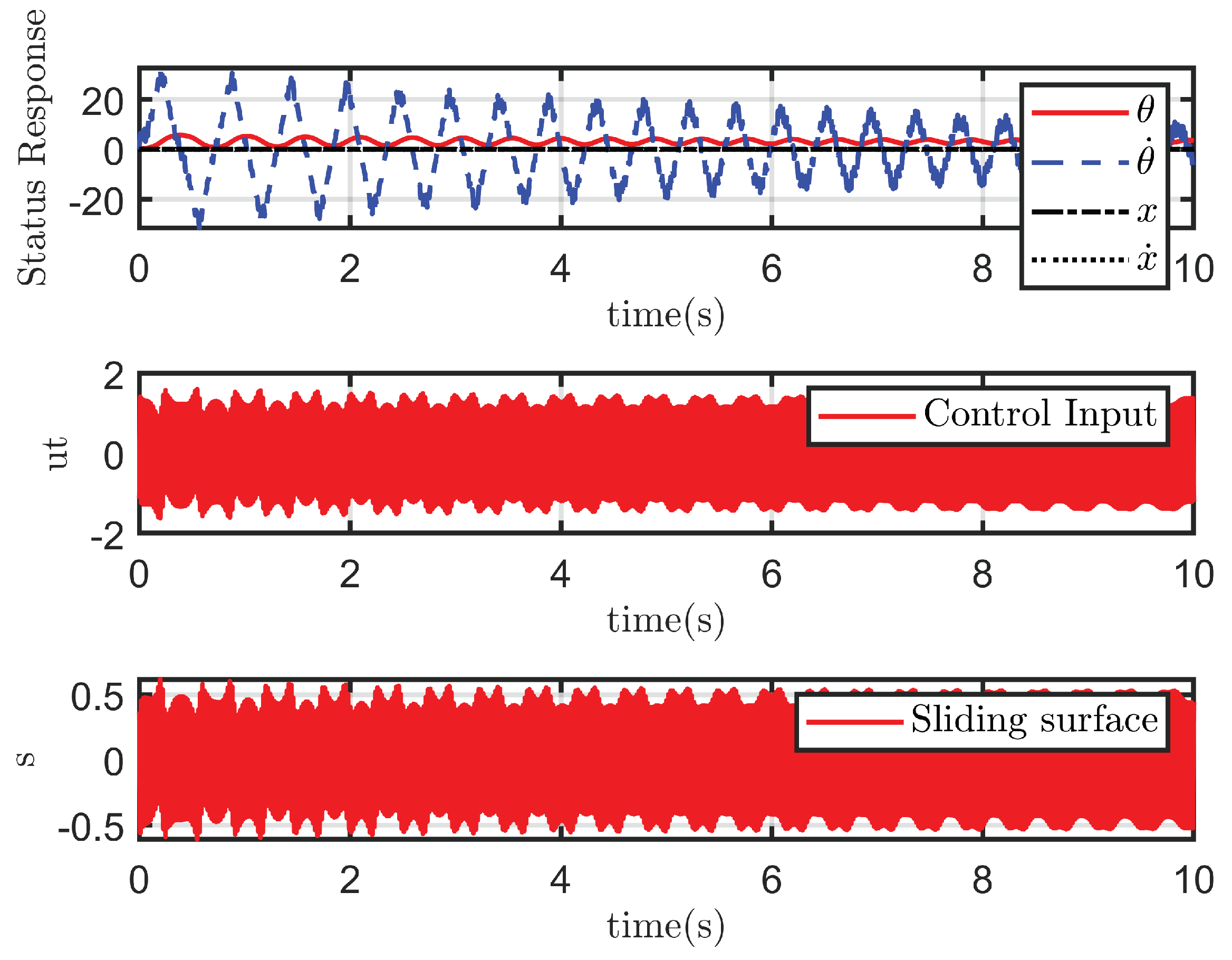
Figure 5.
Performance of HTSMC under JSO optimization algorithm.
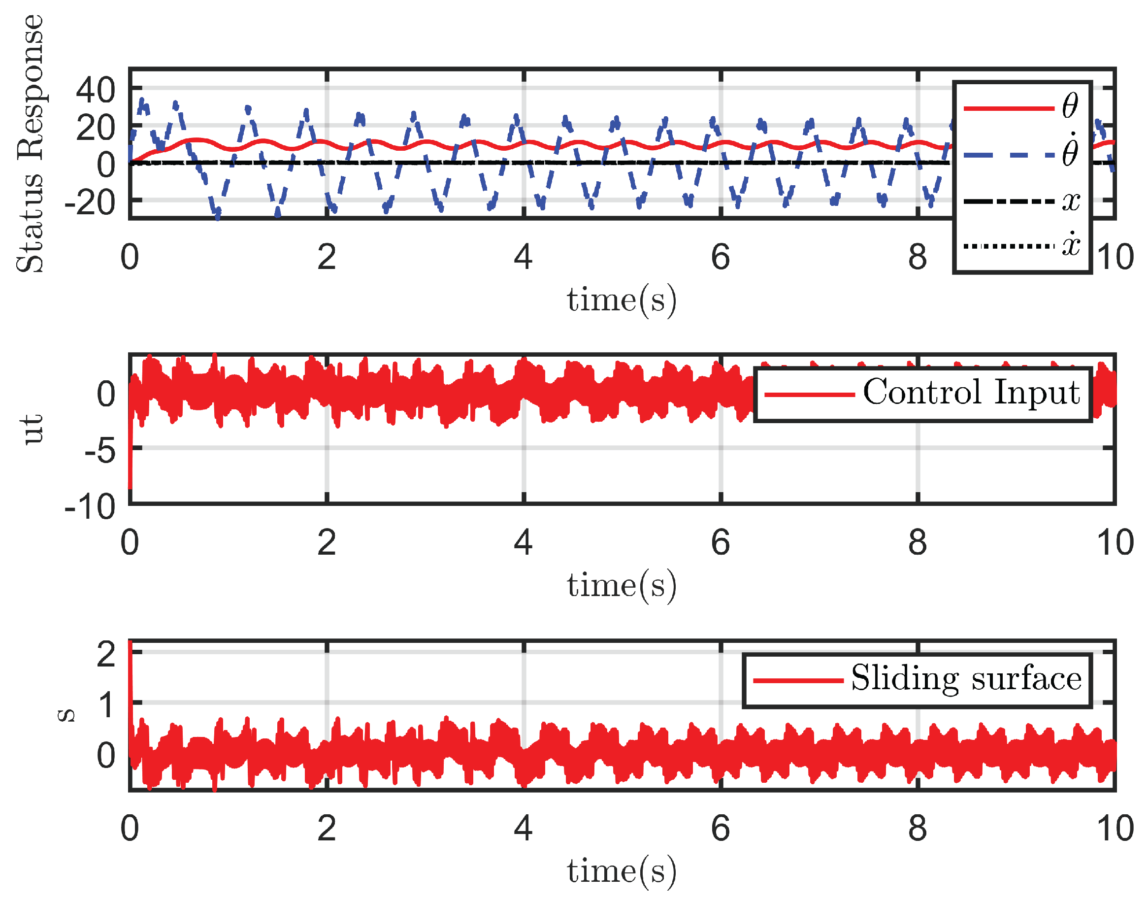
Figure 6.
Performance of MDHTSMC under JSO optimization algorithm.
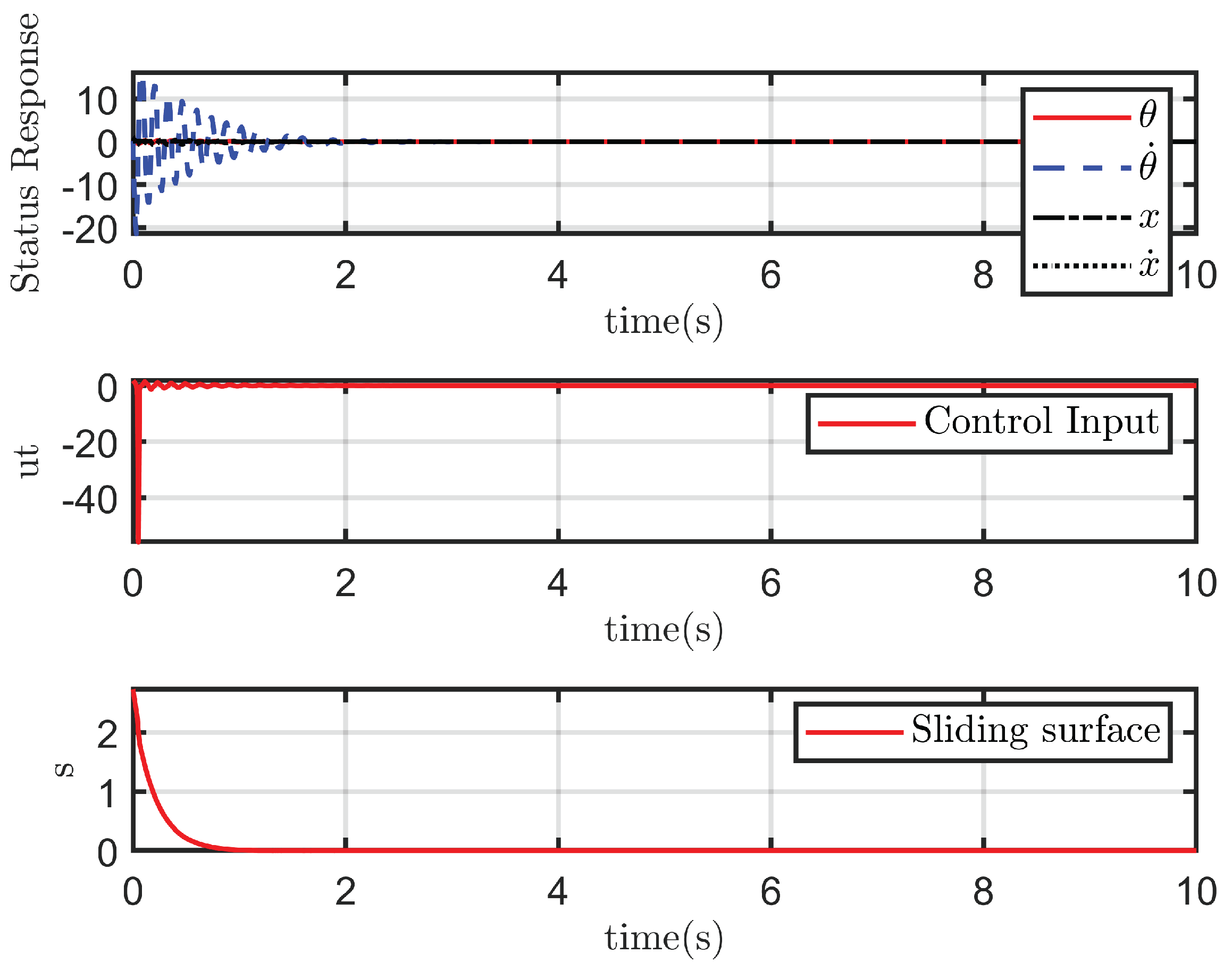
Figure 7.
Performance of HSMC at ideal state.
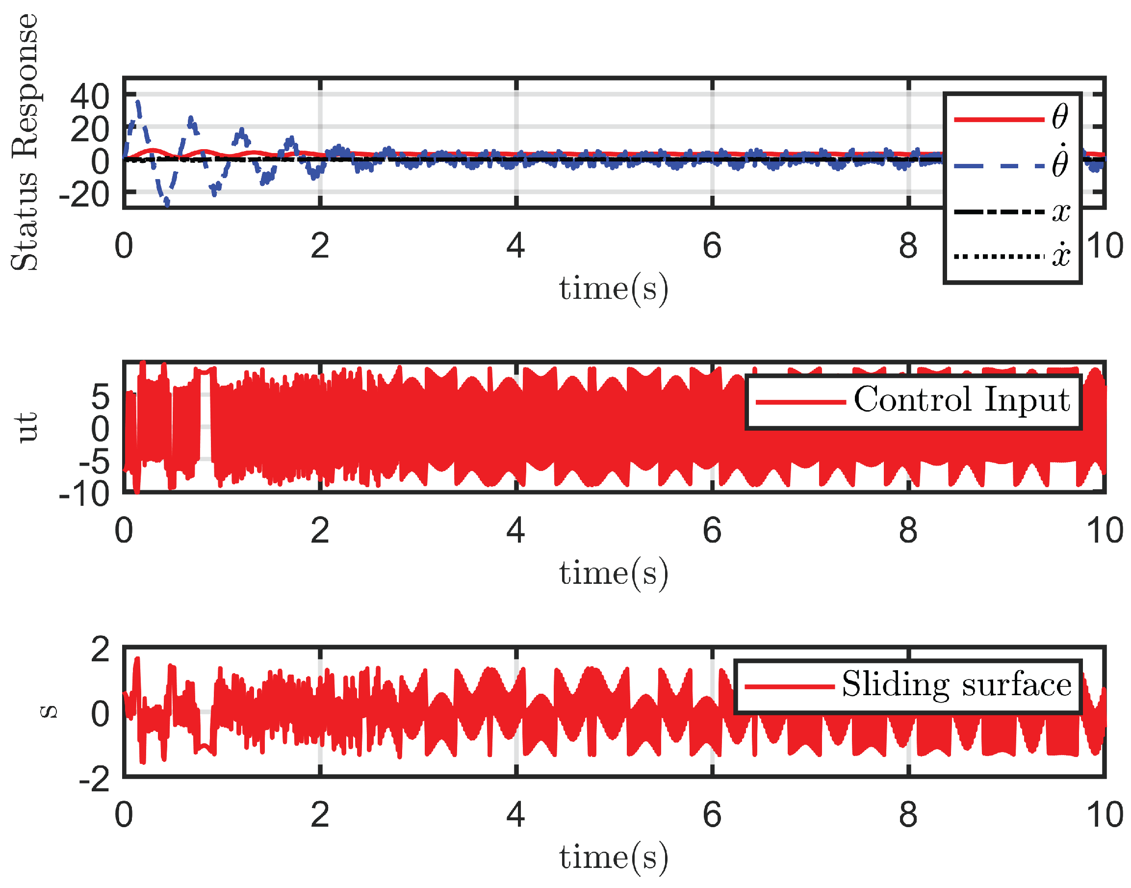
Figure 8.
Performance of HTSMC at ideal state.
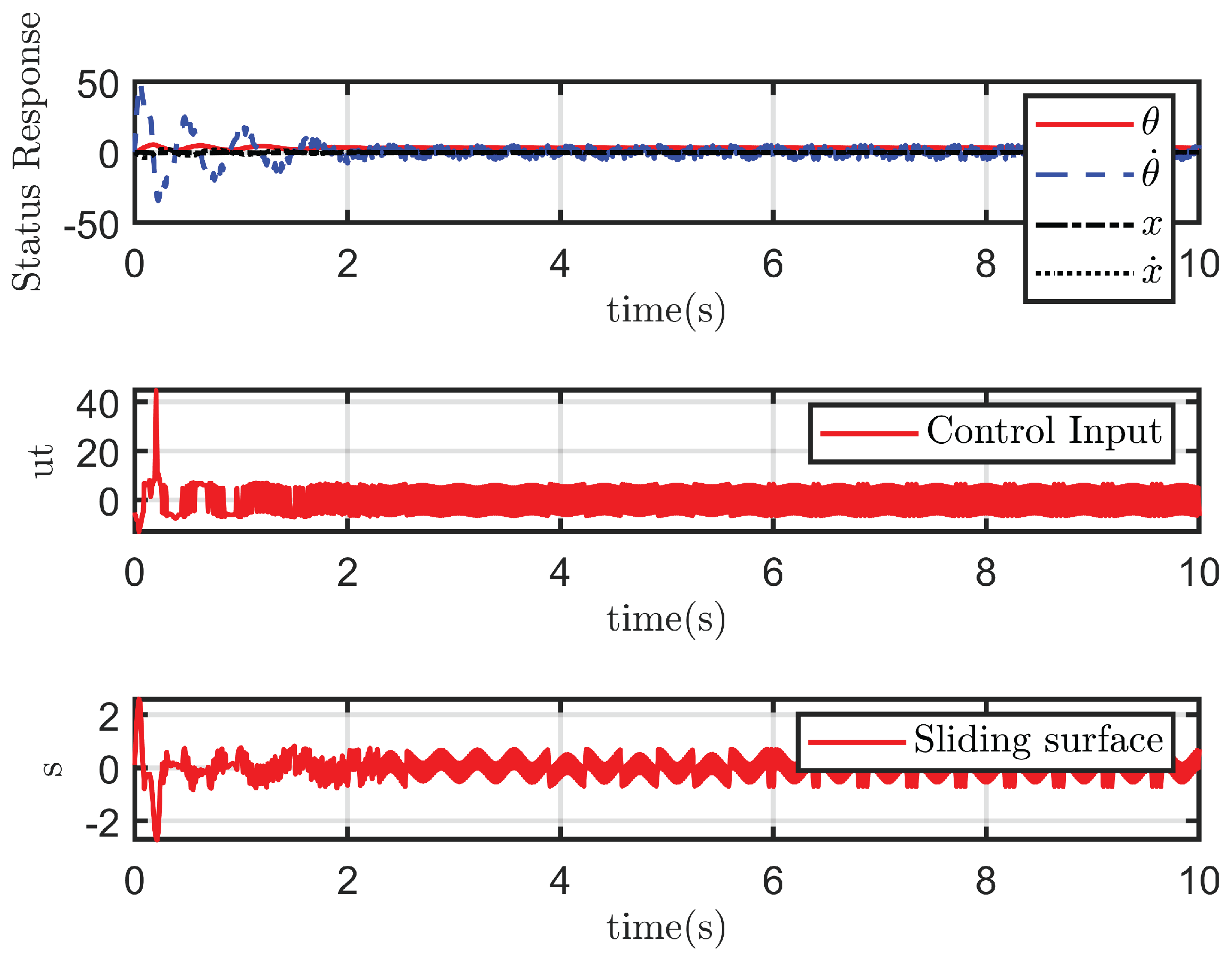
Figure 9.
Performance of MDHTSMC at ideal state.
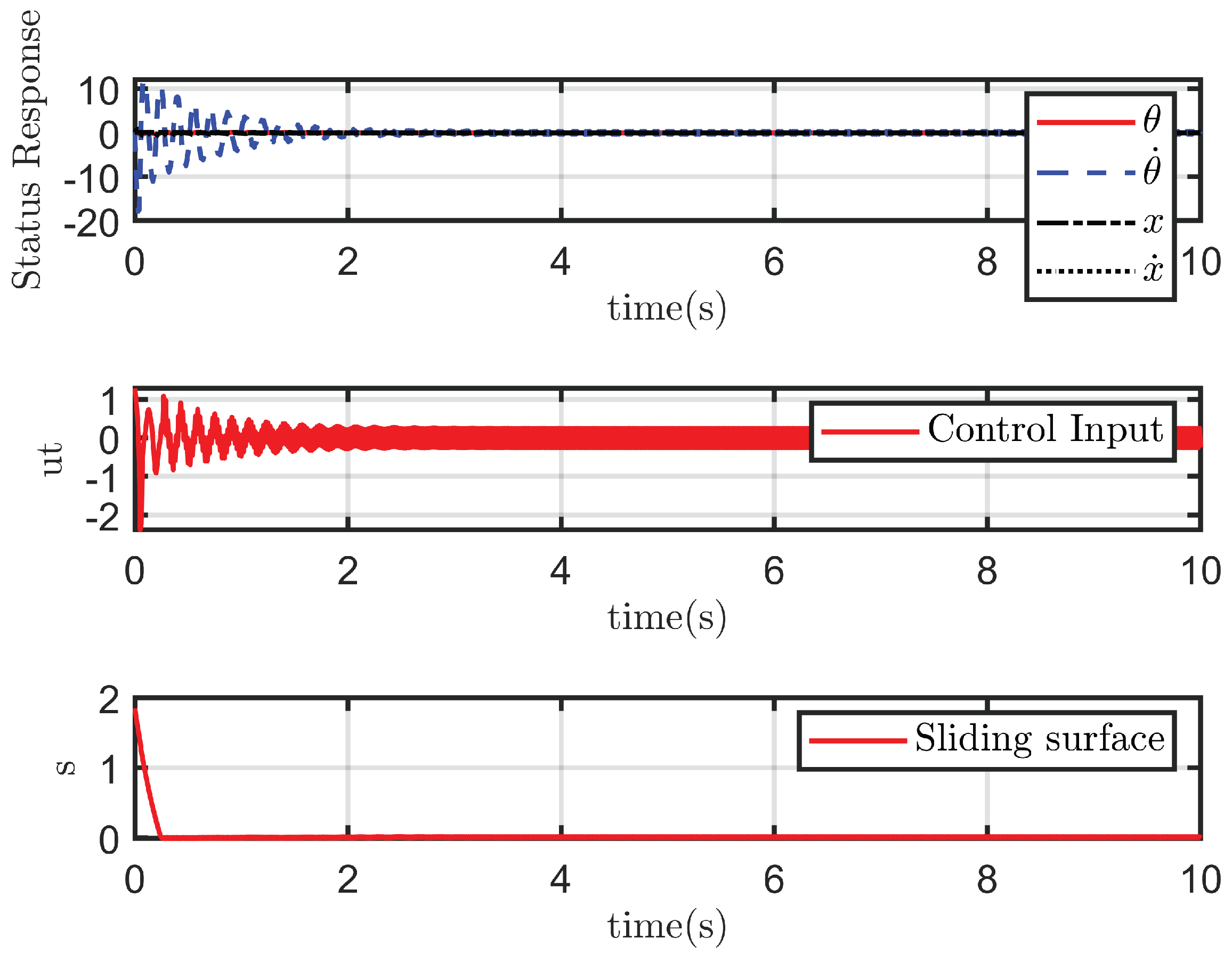
Figure 10.
Performance of HSMC with
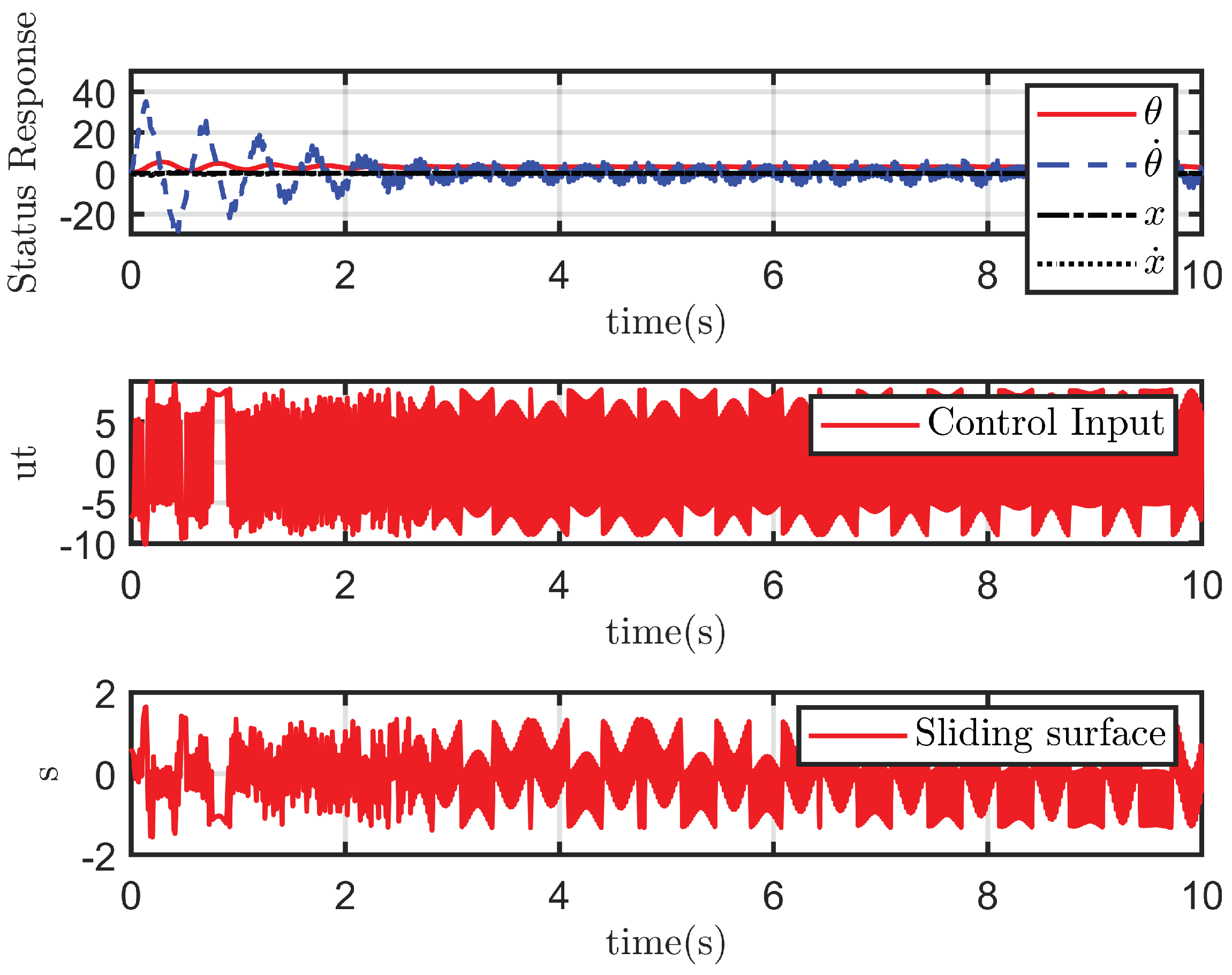
Figure 11.
Performance of HTSMC with
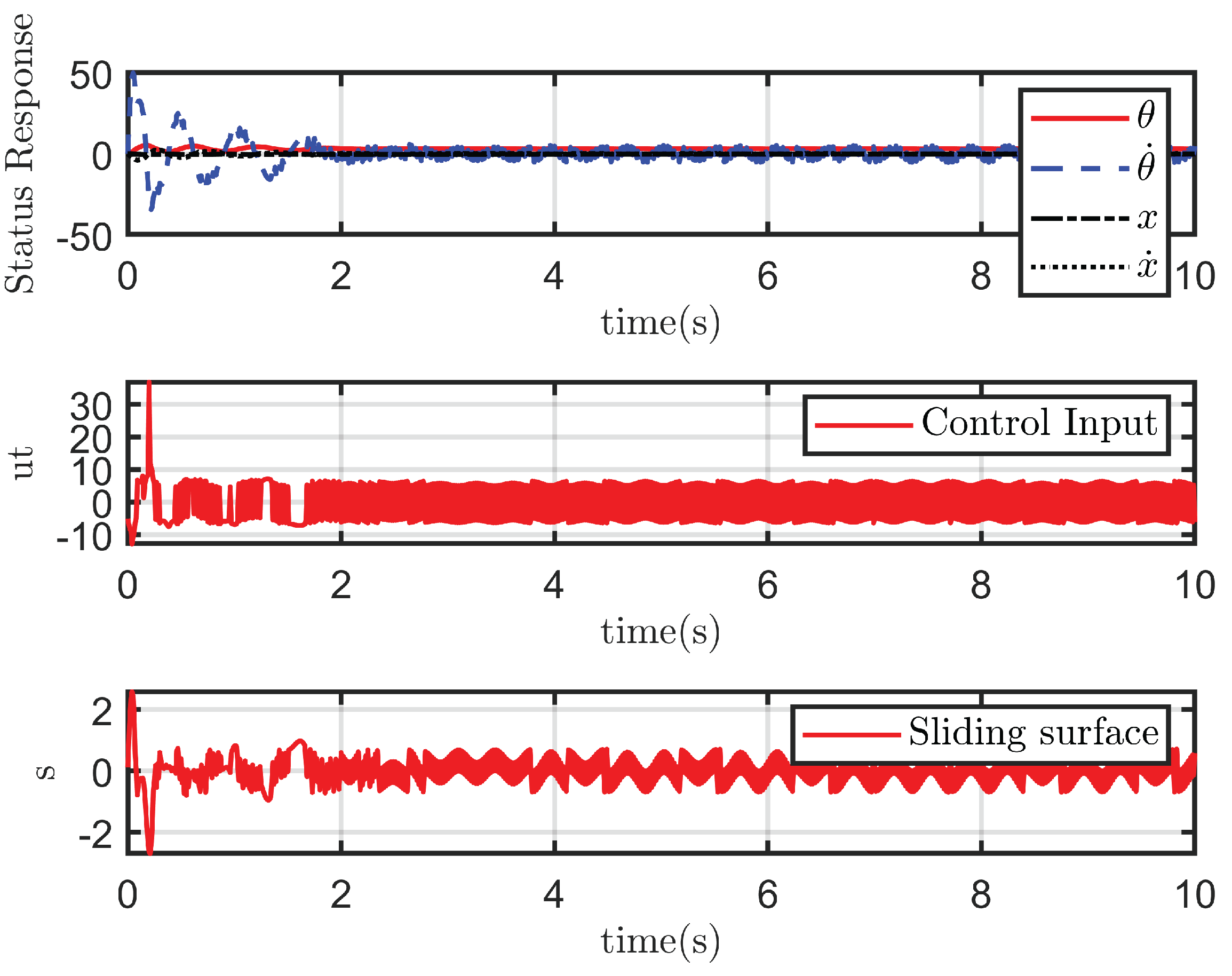
Figure 12.
Performance of MDHTSMC with
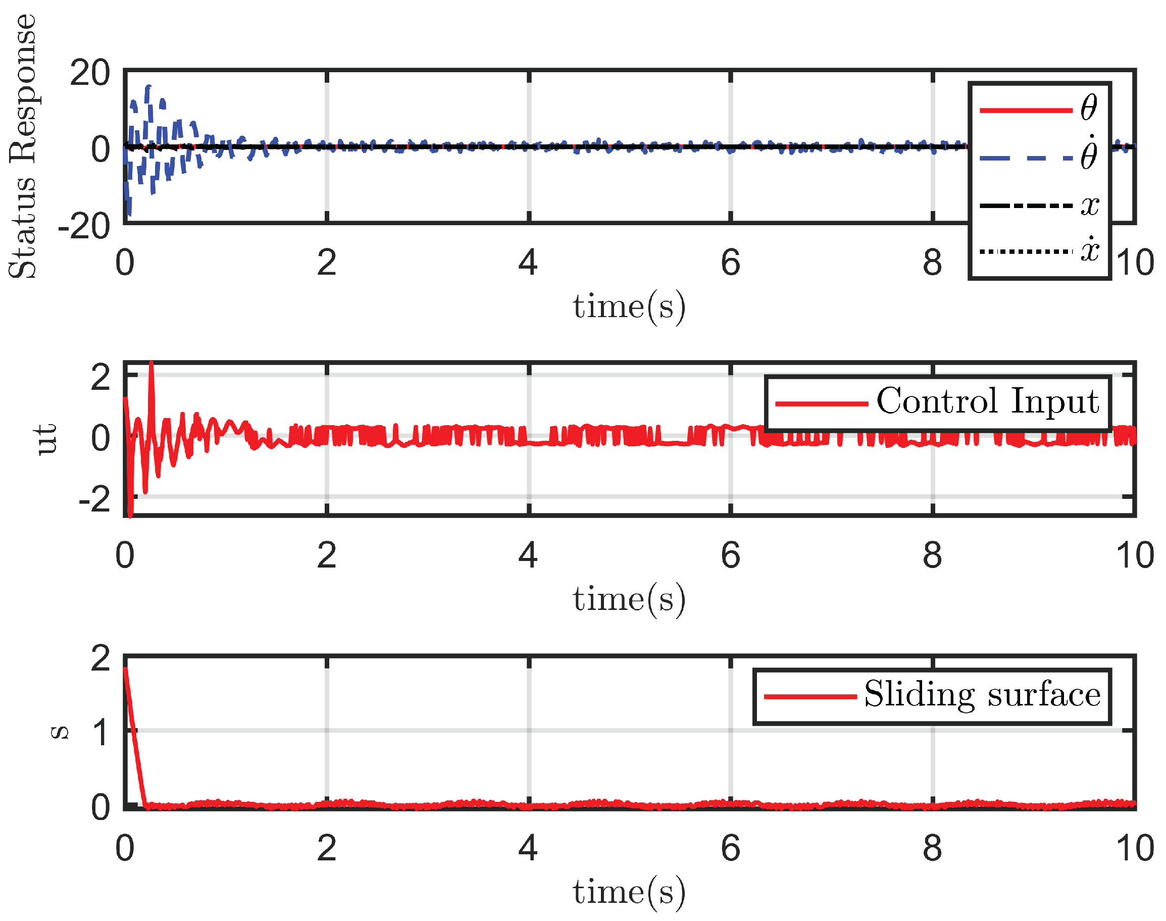

Table 1.
The vehicle parameters and variables.
| Notation | Definition |
|---|---|
| Torques acting on the left and right wheels provided by wheel motors | |
| Interacting forces between the left and right wheels and the chassis | |
| Friction forces acting on the left and right wheels | |
| External forces acting on the left and right wheels | |
| Rotational angles of the left and right wheels | |
| Displacements of the left and right wheels along the x-axis | |
| Tilt angle of the vehicle body | |
| Rotational angle of the vehicle | |
| x | Displacement of the vehicle along the direction of the longitudinal velocity |
| v | Longitudinal velocity of the vehicle |
| m | Mass of the inverted pendulum |
| M | Mass of the chassis |
| Mass of the wheels | |
| R | Radius of the wheels |
| l | Distance between the body center of gravity and the wheel axis |
| D | Distance between the two wheels along the axle center |
| Current position of the vehicle on the plane | |
| Interacting force between the pendulum and the chassis on the x-axis |
Disclaimer/Publisher’s Note: The statements, opinions and data contained in all publications are solely those of the individual author(s) and contributor(s) and not of MDPI and/or the editor(s). MDPI and/or the editor(s) disclaim responsibility for any injury to people or property resulting from any ideas, methods, instructions or products referred to in the content. |
© 2025 by the authors. Licensee MDPI, Basel, Switzerland. This article is an open access article distributed under the terms and conditions of the Creative Commons Attribution (CC BY) license (http://creativecommons.org/licenses/by/4.0/).
Copyright: This open access article is published under a Creative Commons CC BY 4.0 license, which permit the free download, distribution, and reuse, provided that the author and preprint are cited in any reuse.


