Submitted:
19 September 2025
Posted:
19 September 2025
You are already at the latest version
Abstract
Sea surface height (SSH) derived from satellite altimetry is widely used in oceanographic research and marine environmental monitoring. However, numerical ocean models for SSH forecasting are computationally expensive, while purely data-driven methods often lack physical consistency. To address these limitations, we propose a Geostrophic-Constrained Neural Network (GCNN) for short-term SSH prediction in the South China Sea (SCS), utilizing satellite data. Based on the SimVPv2 architecture, the model incorporates several strategies to enhance both physical consistency and forecast performance: (1) using mask information as input to reduce artifacts caused by land contamination in oceanographic data; (2) augmenting the loss function with a physics-informed term that enforces geostrophic balance; and (3) applying latitude-based weighting to this constraint to account for the breakdown of geostrophic approximation near the equator. On the test dataset, the GCNN achieves a root mean squared error (RMSE) of 1.73 cm, representing an 11% improvement over the unconstrained baseline model. Furthermore, the model is computationally efficient, requiring only about 3 hours for training and 3.7 milliseconds per inference. The GCNN not only improves predictive accuracy but also enhances interpretability by adhering to ocean dynamical principles, offering a promising approach for the modeling and prediction of SSH.
Keywords:
Sea Surface Height Forecasting
; Physics-Informed Neural Network
; Geostrophic Constraint
; Deep Learning
; Remote Sensing
1. Introduction
As a critical indicator of mesoscale oceanic dynamical processes, sea surface height (SSH) is routinely used to map mesoscale circulation features [1,2] and quantify mesoscale eddy dynamics [3,4], which contributes to oceanic mass transport comparable in magnitude to that of the large-scale wind- and thermohaline-driven circulation [5]. Given this scientific importance, the ability to accurately forecast SSH is of critical operational and engineering significance. Timely and reliable SSH forecasts provide the basis for deriving surface currents, which are essential for a wide range of maritime activities. In the offshore energy sector, precise knowledge of future current and eddy locations is indispensable for the safe execution of sensitive operations, such as the installation and maintenance of oil rigs and offshore wind turbines [6]. Therefore, developing models that can deliver high-accuracy SSH forecasts is a key objective in modern operational oceanography.
Approaches to forecasting SSH can be broadly categorized into three groups: numerical models, statistical methods, and data-driven deep learning models. Numerical models, such as the Hybrid Coordinate Ocean Model (HYCOM), solve fundamental hydrodynamic equations to simulate oceanic states [7]. While physically comprehensive, they are computationally prohibitive, requiring complex parameterization of sub-grid-scale processes, and the accuracy is highly sensitive to initial and boundary conditions—limitations that have motivated the search for alternative approaches. Statistical methods, such as autoregressive models, offer a computationally cheaper alternative but are often based on linear assumptions, limiting their ability to capture the complex, non-linear dynamics inherent in ocean systems [8].
The rapid development of artificial intelligence (AI) has revolutionized spatiotemporal forecasting in oceanography, with deep learning models emerging as particularly powerful tools. These data-driven approaches have demonstrated remarkable success across various oceanographic applications. Convolutional neural networks (CNNs) have proven effective for El Niño-Southern Oscillation (ENSO) prediction [9], while the integration of multivariate empirical orthogonal function (MEOF) analysis with one-dimensional convolutional long short-term memory (Conv1D-LSTM) networks have shown promising results for multi-variable sea surface forecasting [10]. More recently, innovative adaptations of vision Transformers (ViT) with self-attention mechanisms have enabled three-dimensional multivariate modeling for enhanced ENSO prediction [11].
Despite these advances, fundamental limitations persist in purely data-driven approaches. The inherent “black box” nature of these models raises concerns about physical consistency in their predictions [12], particularly when extrapolating beyond the temporal scope of training data or processing noisy observational inputs. This limitation has motivated the development of Physics-Informed Neural Networks (PINNs), which embed physical laws directly into the learning process through penalty terms that quantify violations of governing equations [13]. The PINN framework has shown considerable promise across various oceanographic applications, including tropical cyclone field reconstruction [14], surface current prediction [15], three-dimensional thermohaline modeling in the tropical Pacific [16], and improved air-sea flux parameterizations [17]. However, despite these successful applications, the potential of PINNs for sea surface height (SSH) forecasting remains largely unexplored, representing a significant gap in current oceanographic research. This gap is particularly noteworthy given SSH’s fundamental role in ocean dynamics through geostrophic balance, a relationship that could provide natural physical constraints for PINN-based forecasting systems.
Building on this potential, we note that among the fundamental principles of ocean dynamics, the geostrophic balance provides a robust first-order approximation for large-scale, low-frequency ocean circulation. This balance, which describes an equilibrium between the Coriolis force and the pressure gradient force, is known to govern the circulation in many regions of the world’s oceans [3]. The South China Sea (SCS) is one such region, where the large-scale circulation is predominantly in geostrophic balance [18,19]. A key practical advantage of using a geostrophic constraint is its elegance and efficiency: it relates the sea level gradient to the velocity field, meaning the constraint can be formulated using only SSH data, without requiring external variables like wind forcing or in-situ velocity measurements.
In this study, we propose and evaluate a Geostrophic-Constrained Neural Network (GCNN) for ten-day SSH forecasting in the SCS. A latitude-weighted geostrophic constraint is embedded into the loss function, along with the incorporation of mask information, to further enhance model performance. Our primary objective is to demonstrate that this physics-informed approach improves both forecast accuracy and physical consistency compared to a purely data-driven baseline. In addition to extensive experiments validating the model’s improvement, we conduct a comprehensive analysis of its performance across different seasons, forecast lead times, and bathymetric regimes. This analysis aims to quantify the benefits and limitations of applying the geostrophic constraint in this dynamically complex region.
2. Data and Methods
2.1. Data
This study employs daily mean absolute dynamic topography data—defined as the sea surface height above the geoid and hereafter referred to as SSH—obtained from the Copernicus Marine Environment Monitoring Service (CMEMS). The dataset has a spatial resolution of 1/8° × 1/8° and incorporates multi-satellite altimeter observations. It has undergone tidal correction and mean dynamic topography processing to ensure data quality.
The study domain (2°N–22°N, 104°E–124°E) encompasses the SCS basin and adjacent Luzon Strait, corresponding to a 160×160 grid. This region captures critical dynamical features including the Kuroshio intrusion through Luzon Strait, which significantly modulates SCS circulation patterns (Nan et al., 2015) and consequently influences SSH variability across the basin. The dataset covers the period from 1 January 1993 to 14 June 2024 and is divided into three subsets: a training set (1993–2021), a validation set (2022), and a test set (2023–14 June 2024). The validation set is used for hyperparameter tuning and monitoring the training process, while the test set serves as an independent dataset to evaluate the model’s predictive performance. Notably, 2022 was a La Niña year, whereas 2023 transitioned to an El Niño year. Previous studies have demonstrated that ENSO signals can influence SCS circulation and SSH variability through processes such as the Luzon Strait water exchange [20]. This interannual variability introduces additional challenges for model predictions but provides a more rigorous assessment of the model’s generalization capability.
2.2. Model
2.2.1. Model Structure
The SimVPv2 model employed in this study is a purely convolutional architecture that efficiently captures spatiotemporal coupling relationships through a gated spatiotemporal attention (gSTA) mechanism. Compared to conventional spatiotemporal prediction models (e.g., ConvLSTM [21], PredRNN [22]), SimVPv2 demonstrates superior performance in terms of structural simplicity, computational efficiency, and prediction accuracy, showing exceptional performance on multiple benchmark datasets [23]. These characteristics make it particularly suitable for modeling complex oceanographic data.
Designed for sequential prediction of two-dimensional spatial variables, the SimVPv2 architecture consists of three primary components: (1) Spatial Encoder, (2) Spatiotemporal Translator, and (3) Spatial Decoder. Similar to U-Net, the model incorporates skip connections between the initial encoder layers and final decoder layers to preserve original features.
The Spatial Encoder comprises Nₛ layers of 2D convolutional blocks, each defined as:
where zᵢ represents the feature map after the i-th convolutional block (with z₀ as input), Conv2d denotes a standard 3×3 2D convolution (implemented as PyTorch’s Conv2d), Norm2d indicates a GroupNorm layer (group=2), and σ represents the SILU activation function. The architecture alternates between stride=1 and stride=2 convolutions for progressive downsampling.
The Spatial Decoder essentially mirrors the structure of the encoder, replacing downsampling operations with upsampling through PyTorch’s PixelShuffle using a scale factor of 2. The final layer serves as the output layer, which converts the feature channels into the desired number of output channels.
The core part lies in the Spatiotemporal Translator, composed of Nₜ stacked gSTA Blocks. As illustrated in Figure 1, each gSTA Block sequentially combines a Spatial Attention layer and a MixMLP layer (constructed from 1×1 convolutions and depth-wise convolutions). The Spatial Attention layer features channel-preserving 1×1 convolutions bracketing an attention module, and the attention module can be mathematically expressed as:
where and denote depthwise and dilated depthwise convolutions respectively, g represents attention coefficients, σ indicates softmax normalization, and ⊙ is element-wise multiplication. This gating mechanism dynamically weights features based on their spatiotemporal importance.
2.2.2. Hyperparameter Configuration
For an input tensor of dimensions , the model first flattens the temporal dimension into the batch dimension . After spatial encoding, the tensor undergoes channel-temporal folding to , where and . The translator’s operations on this restructured tensor enable simultaneous learning of spatial and temporal relationships through depthwise spatial attention and channel-wise convolutions.
As shown in Figure 2, we adopt a 10-day sequence of SSH fields as input to predict the subsequent 10-day SSH fields, corresponding to input and output dimensions of (10, 1, 160, 160). Given the relatively low spatial resolution (160×160), we minimize information loss during downsampling and upsampling by limiting the encoder layers (Ns) to 2, performing only one downsampling and one upsampling operation. Within the attention module, we employ dilated convolutions with a dilation rate of 2 (skipping every other grid point) and an effective kernel size of 21 to capture broader spatial dependencies.
To enhance computational efficiency and mitigate overfitting —constrained by the small training dataset (several thousand samples) and low data resolution—we select conservative hidden layer dimensions: a spatial hidden size of 16 and a temporal hidden size of 128. Further regularization is achieved via dropout and drop path rates of 0.3. Other hyperparameters, including the default kernel size 3 for encoder/decoder convolutions and the MLP ratio 8 in the Translator’s MixMLP, remain unchanged.
The training was conducted on an NVIDIA GeForce RTX 4090 GPU with 24 GB of memory. To mitigate overfitting and improve computational efficiency, the following training strategy was adopted: a batch size of 4 was used to introduce more stochasticity and accelerate training. A ReduceLROnPlateau learning rate scheduler was applied with an initial rate of 1e⁻⁴ to alleviate gradient instability caused by the small batch size. The learning rate was reduced by a factor of 0.1 if the validation loss did not decrease for 5 consecutive epochs, thereby promoting steady convergence. Training proceeded for up to 150 epochs with early stopping configured with a patience of 10 epochs, monitoring the validation loss to terminate training if no improvement was observed.
Under the specified configuration, the GCNN model is relatively compact with only 3,273,809 parameters. Training was completed in approximately three hours, processing samples at an average rate of 64.4 samples per second. During testing, the model demonstrated efficient inference, with an average latency of 3.7 milliseconds per sample — a value derived from averaging over 10,000 inference runs at a batch size of 1. The entire process required only a single RTX 4090 GPU, highlighting its computational efficiency and low resource demands.
2.3. Strategies
2.3.1. Geostrophic Constraint in SSH Prediction
In physical oceanography, the geostrophic balance is a fundamental dynamical approximation in which the Coriolis force is balanced by the horizontal pressure gradient force. Owing to its clear physical meaning and relatively simple mathematical form, it is widely used to estimate large-scale oceanic currents from sea surface height (SSH) observations.
Under the f-plane approximation, where the Coriolis parameter is assumed constant, the geostrophic balance can be expressed as:
where () are the zonal and meridional components of the geostrophic velocity, g is the gravitational acceleration (taken as 9.81 m/s-2), ζ represents the sea surface height (SSH), and f is the Coriolis parameter, defined as:
Here, Ω is the Earth’s angular velocity (taken as 7.2921×10⁻⁵rad/s), and ϕ is the latitude.
Solving equations (5) and (6) for the velocity components yields:
In the training of our SSH prediction model, both the input and output are exclusively SSH fields. The primary loss function is the Mean Squared Error (MSE) between the predicted and target SSH:
Here, denote the predicted SSH and the target SSH from the training dataset for the corresponding date, respectively. The MSE is calculated as:
where N is the total number of data points.
To incorporate the geostrophic balance into the model’s loss function, a geostrophic constraint loss is introduced. First, the SSH spatial gradient fields of predictions and targets are computed using a Sobel operator. Subsequently, the geostrophic velocity components () are derived from the SSH spatial gradient fields as described in equations (8) and (9). The calculated geostrophic velocities are divided by the standard deviation from CMEMS geostrophic velocity data and multiplied by that from CMEMS SSH data—a step intended to align the dimension of the computed geostrophic velocities with that of SSH. Finally, the MSE between the predicted and target geostrophic velocities forms the geostrophic loss term:
The total loss function for training the model is a linear combination of the SSH prediction loss and the geostrophic velocity loss:
where λ is the geostrophic constraint coefficient. A larger value of λ imposes a stronger geostrophic constraint, whereas a smaller value signifies a weaker constraint.
2.3.2. Latitude-Weighted Loss
The geostrophic constraint in our model is based on the geostrophic velocity equations (Eq. 8, 9). A direct application of these equations is problematic at low latitudes, as the Coriolis parameter f in the denominator approaches zero, leading to an over-amplification of the geostrophic loss term where the geostrophic balance is inherently weak. This can introduce significant errors into the model training process.
To mitigate this issue, we introduce a latitude-dependent weighting factor, w(ϕ), designed to smoothly suppress the geostrophic constraint in equatorial regions. The weight is calculated using the following square rooted sigmoid function:
According to Lagerloef et al. (1999), the geostrophic approximation under the f-plane assumption is generally valid at latitudes higher than approximately 5°N. Based on this guidance, we introduce a latitude-dependent weighting scheme to gradually apply the geostrophic constraint with increasing latitude. Specifically, we define a sigmoid-shaped weight function with parameters and k = 2, such that the weight transitions smoothly from nearly 0 south of 5°N to nearly 1 north of 10°N.
2.3.3. Mask-Informed Input
In the application of deep learning models, particularly convolutional neural networks, to oceanographic data, a significant challenge is the prevalence of NaN (Not a Number) values—which often correspond to land grids in marine datasets. A common practice is to replace these NaN values with zeros. However, this approach is suboptimal, as simply zero-filling may mislead the convolutional model during feature extraction, given that such models rely on sliding kernels across the grid to capture meaningful spatial patterns. Another method involves interpolation, which fills the land grids using values derived from surrounding ocean data. While interpolation may offer better performance than simply assigning zeros to land grids, it still introduces misleading information to the model: originally information-free land areas are now filled with artificially imputed values, which do not correspond to any real physical processes and may still distort feature learning.
For instance, in SSH prediction tasks, shallow network layers could misinterpret zero-filled or interpolated land grids as authentic SSH values, thereby propagating erroneous information to deeper layers. To address this issue, we propose a simple yet effective method: concatenating a binary mask that identifies valid grids—a tensor of ones and zeros with the same spatial dimensions as the input, but with a single channel—to the input along the channel dimension. This operation transforms the input shape from (B, T, C, H, W) to (B, T, C+1, H, W), thereby explicitly informing the model about the presence of invalid grid cells in a straightforward yet effective manner.
3. Results
3.1. Impact of the Geostrophic Constraint Coefficient
To determine the optimal weighting for the geostrophic constraint, we conducted a series of experiments in which the model was trained under varying values of the geostrophic constraint coefficient, denoted as . In order to mitigate the effects of randomness and enhance the robustness of the results, each experiment was repeated five times under identical hyperparameter settings except for the random seed. The performance of each configuration was evaluated on the test dataset, and the results were averaged across the five runs to ensure a more reliable and statistically meaningful comparison.
Figure 3 illustrates the relationship between model performance and λ, using the RMSE and the Pearson Correlation Coefficient (PCC) as evaluation metrics. RMSE is computed as the square root of the mean squared error between predicted and target SSH fields, averaged over the test set, while PCC is calculated by averaging the daily correlation coefficients between predicted and target SSH fields across the test set. As λ increases from zero, the RMSE initially decreases and the PCC increases, indicating improved performance. Optimal performance is achieved at λ = 0.7, after which the model’s accuracy degrades. Therefore, the term GCNN hereafter refers specifically to the model trained at this optimal value (λ = 0.7).
Given that the geostrophic loss were normalized, the coefficient λ can be interpreted as the relative importance assigned to the geostrophic loss versus the primary SSH loss. The degradation in performance for λ > 0.7 suggests that the geostrophic constraint should serve as a supplementary, rather than dominant, component of the loss function. This phenomenon can be mainly attributed to the presence of ageostrophic dynamics: Ocean circulation is not exclusively geostrophic; it contains significant ageostrophic components. A key advantage of data-driven models is their ability to learn complex relationships not fully captured by simplified physical equations. Forcing the model to adhere too strictly to geostrophy by increasing λ penalizes it for learning these true, non-geostrophic dynamics. This rigid constraint becomes counterproductive, leading to performance that can be worse than that of the unconstrained AI model.
3.2. Ablation Study
In the Method section, we introduced three strategies aimed at enhancing model performance. As demonstrated in Figure 3, integrating all three leads to notable improvement. However, the individual contribution of each strategy had not been evaluated. To assess their respective effectiveness, we conducted a series of ablation studies in which one strategy was omitted at a time. As shown in Figure 4, the removal of any of the three strategies results in an increase in RMSE and a decrease in PCC. Among them, abandoning the geostrophic constraint has the most pronounced effect. These results confirm that all three strategies contribute to improving the performance of the GCNN, and that the geostrophic constraint plays an especially critical role.
4. Analysis of Results
Authors should discuss the results and how they can be interpreted from the perspective of previous studies and of the working hypotheses. The findings and their implications should be discussed in the broadest context possible. Future research directions may also be highlighted.
From the experiments above, it can be observed that the fluctuations caused by randomness during the training process are considerable. To minimize the impact of such randomness, all random seeds were fixed to 42 and cuDNN’s deterministic algorithms were enabled throughout the training of the subsequent models. This ensures that models trained under the same hyperparameters are strictly identical, except for those trained with geostrophic constraint loss. Due to its additional computational steps, this loss introduces new uncertainties. Nevertheless, as Table 1 demonstrates, despite not being entirely identical, the use of fixed random seeds and cuDNN’s deterministic algorithms still results in highly consistent GCNN outputs across repeated trials under identical hyperparameters. Across three independent trials, the RMSE values exhibit minimal deviation, remaining within 1.6% of the mean RMSE. Based on this high consistency, we selected one of the three runs as the representative instance of the GCNN for all subsequent analyses.
4.1. Comparative Performance Analysis
To further evaluate the effectiveness of the physics-informed approach, the performance at different lead time of the GCNN was compared against two other models: Base and Persistence. Persistence, which assumes the future state is identical to the current state (ζ(t+1) = ζ(t)), is a benchmark comparison and forecast reference widely accepted in oceanic science [24], and serves as a simple baseline for forecast skill here.
As shown in Figure 5, both the GCNN and Base significantly outperform Persistence in terms of RMSE, with the performance gap widening as the lead time increases. A similar trend is observed for the PCC. While Persistence’s correlation is comparable to the AI models at a lead time of one day, its performance degrades rapidly thereafter, highlighting the superior predictive skill of the GCNN at longer horizons.
Most importantly, the GCNN consistently demonstrates improved performance over the Base, exhibiting lower RMSE and higher PCC across all lead times. This result confirms the benefit of incorporating physical knowledge into the neural network architecture. However, the magnitude of this improvement is modest. This is likely attributable to the challenges of applying the geostrophic constraint over a domain that includes extensive low-latitude areas where the geostrophic balance is weak. Although the latitude-weighting scheme was implemented to mitigate this, it may introduce discontinuities in the loss function that can complicate the training process, thereby limiting the full potential benefit of the physical constraint.
4.2. Seasonal Variation in Prediction Accuracy
The predictive performance of both the Base and the GCNN exhibits a distinct seasonal cycle, as illustrated in the time series of forecast errors in Figure 6. For this analysis, the error metric for any given start date represents the average performance over the subsequent ten-day forecast period. Figure 6 clearly indicates that for both models, the RMSE and the PCC are both systematically lower during the summer months (April–September, red shading) compared to the winter months (October–March, blue shading).
We hypothesize that this seasonal difference in forecast skill is primarily driven by the inherent seasonal variability of the SSH field itself. To investigate this, we quantified the temporal and spatial variability of SSH for each season in the test dataset. Mean Temporal variability, denoted as , is defined as the spatial average of the standard deviation calculated over time at each grid point. It measures the typical magnitude of temporal fluctuations within the SSH field. Mean Spatial Variability, denoted as , is defined as the standard deviation of the time-averaged SSH field. It represents the magnitude of spatial fluctuations within the time-averaged SSH field.
As summarized in Table 2, both the mean temporal and spatial variability are significantly lower in summer than in winter. This indicates that the SSH field is generally more quiescent and spatially smoother during the summer. To directly link this variability to prediction error, we computed the PCC between the temporal variability () and the time-averaged absolute error (AE) of the Base prediction at each grid point. The analysis revealed statistically significant positive correlations in both summer (r = 0.52) and winter (r = 0.58), with confidence levels exceeding 99.9%. This confirms that locations with greater temporal variability are inherently more difficult to predict, and that the higher overall variability in winter is a key driver of the observed seasonal degradation in forecast accuracy. Combined with the stronger correlation in winter, we hypothesize that the SSH field exhibits more high-frequency and irregular variations in winter, leading to a greater tendency of the model to overfit. This overfitting contributes to the seemingly counterintuitive phenomenon whereby both RMSE and PCC are higher in winter than in summer.
Furthermore, a closer inspection of Figure 6 reveals that the performance improvement of the GCNN over the Base is more pronounced in summer, especially when the lead time is longer. This observation aligns with established ocean dynamics in the SCS. The summer period is characterized by more stable large-scale geostrophic circulation patterns [25]. In this regime, the geostrophic constraint provides a more accurate and beneficial physical prior. In contrast, winter is typically marked by stronger wind forcing and enhanced Ekman dynamics, which disrupt the geostrophic balance, particularly in the upper ocean [26]. The reduced validity of the geostrophic assumption in winter likely limits the effectiveness of the physics-informed constraint, resulting in a smaller performance gain for the GCNN.
4.3. Spatial Distribution of Forecast Error
The previous section established that the overall forecast error is lower in summer and that the performance improvement of the GCNN is also season-dependent. To further investigate these patterns, we analyze the spatial distribution of the time-averaged absolute error (AE) for both the Base model and the GCNN, as shown in Figure 7 and Figure 8.
Figure 7 indicates that the AE of the Base model is not uniformly distributed, with elevated errors concentrated in dynamically active regions, including the coastal waters off Vietnam, the Gulf of Tonkin, the Guangdong coast, the area east of the Luzon Strait, and the Sunda Shelf.
Further analysis of Figure 8 reveals that the AE of the Base model is initially relatively uniform but becomes increasingly heterogeneous as lead time increases. This inhomogeneity also exhibits seasonal variations. For example, at a lead time of 10 days, the AE is notably higher during winter along the Vietnamese coast, the Guangdong coast, the Gulf of Tonkin, and the Sunda Shelf. This pattern is consistent with the winter intensification of monsoon-driven circulation features, such as the Vietnam Coastal Current and the Natuna Eddy, which are associated with stronger nonlinear dynamics [27].
In addition to seasonal variations, another prominent characteristic of the forecast error is the strong influence of bathymetry. High-error regions are predominantly located in shallow coastal and shelf waters. To quantify this, we divided the domain into shelf areas (< 200 m) and deep-basin regions (DB; defined as areas with water depth exceeding 200 m). As summarized in Table 3, the RMSE for the Base model in the DB region is 1.717 cm, which is 13% lower than the full-domain RMSE of 1.977 cm. This discrepancy can be attributed to two main factors: (1) the reduced accuracy of satellite altimetry data in coastal zones [28], and (2) the presence of complex nearshore dynamical processes—such as coastal currents, shelf waves, tides, and upwelling—which are often nonlinear, high-frequency, and not fully resolved by the model [29].
4.4. Impact of the Geostrophic Constraint
The application of the geostrophic constraint also leads to significant spatial variation in forecast performance. As indicated in Table 3, the improvement achieved by the GCNN over the Base model is more pronounced in the DB region, where the RMSE is reduced by 16%, compared to a 12% reduction in the whole domain (WD).
Figure 7 shows that the GCNN improves forecast accuracy across most of the study areas. One of the most substantial improvements occurs east of the Luzon Strait. This result aligns with previous studies suggesting that the Kuroshio transport through the strait is primarily governed by geostrophic dynamics [30], confirming that the integration of this physical constraint enhances model performance in regions where the underlying assumption is most valid.
The effect of the geostrophic constraint also varies with forecast lead time (Figure 8). At a one-day lead time, the GCNN provides relatively uniform improvement across the domain. However, as the lead time extends to 7 and 10 days, the spatial distribution of improvements becomes more heterogeneous. While performance gains intensify in regions where geostrophic balance dominates—such as east of the Luzon Strait and the central deep basin—some areas near the land boundary show limited improvement or even increased error. This may be related to complex nonlinear effects induced by boundary dynamics, which warrant further investigation.
5. Conclusions
In this study, we developed a physics-informed deep learning model, termed the Geostrophic-Constraint Neural Network (GCNN), to improve sea surface height (SSH) forecasting in the South China Sea (SCS). Based on the SimVPv2 architecture, the GCNN incorporates two key enhancements: First, it uses mask information as input to reduce artifacts introduced by the processing of extensive land points in oceanographic datasets with AI models. Second, a latitude-weighted geostrophic constraint is integrated into the loss function by minimizing the discrepancy between predicted and target geostrophic currents derived from SSH gradients. This constraint accounts for the reduced validity of geostrophic balance near the equator. By embedding these first-order physical dynamics, the model achieves improved forecast accuracy and enhanced physical consistency without increasing computational complexity during prediction.
We investigated the influence of seasonality on model performance. Both the Base and GCNN models demonstrated higher forecast accuracy during summer compared to winter. Correlation analysis between the AE of the Base prediction and temporal variability of the SSH field confirmed that regions with higher temporal variability are inherently more challenging to predict. Consequently, the increased temporal variability of SSH during winter is identified as a significant factor contributing to seasonal degradation in forecast accuracy. Further evaluation revealed that the GCNN consistently outperformed the Base in RMSE, with more substantial improvements during summer (14%) compared to winter (10%). This seasonal discrepancy is likely attributable to more stable and geostrophically consistent circulation patterns during the summer southwestern monsoon.
Bathymetric effects were also investigated. Both models exhibited significantly lower RMSE in deep basin areas (DB, depth > 200 m) compared to the whole domain—a result primarily attributable to two factors: the reduced accuracy of satellite altimetry data in coastal zones, and the presence of complex nearshore dynamical processes not fully captured by the models. Moreover, the performance advantage of the GCNN over the Base was more pronounced in DB. These results underscore the role of topographic features in modulating the efficacy of physical constraints, highlighting the necessity of incorporating bathymetric context into the design of future models.
Overall, this study confirms the feasibility and value of embedding geophysical constraints, specifically geostrophic balance, into deep learning frameworks for SSH forecasting. GCNN improves prediction skill while enhancing interpretability by aligning with physical ocean dynamics. This work demonstrates a promising direction for integrating physical knowledge with data-driven modeling in ocean prediction.
As previous studies have shown that wind forcing plays a critical role in modulating SCS circulation, our future research will focus on incorporating wind stress fields as predictive inputs. Integrating wind fields could further enhance model performance in regions where Ekman dynamics and wind-driven processes dominate SSH variability. This extension may also enable better forecasting of wind-induced coastal currents and mesoscale eddies, with potential applications in real-time navigation, marine hazard early warning, and coupled atmosphere–ocean modeling.
Author Contributions
Conceptualization, L.H. and Y.S.; methodology, L.H.; software, L.H.; validation, L.H. and D.L.; formal analysis, L.H.; investigation, L.H.; resources, Y.S. and J.Y.; data curation, L.H. and J.Y.; writing—original draft preparation, L.H.; writing—review and editing, L.H., Y.S., J.Y., and D.L.; visualization, L.H.; supervision, Y.S.; project administration, L.H. and J.Y.; funding acquisition, J.Y. All authors have read and agreed to the published version of the manuscript.
Funding
This research was funded by the China Meteorological Administration, grant number 2024-K-03, the National Natural Science Foundation of China, grant number 42076201, and the Program of the Chinese Academy of Sciences, grant number 133244KYSB20210026.
Data Availability Statement
The datasets analyzed in this study are publicly available at https://doi.org/10.48670/moi-00148, accessed on 18 May 2025.
Acknowledgments
The numerical simulations in this study were supported by the High-Performance Computing Division of the South China Sea Institute of Oceanology, for which we express our sincere gratitude. We also acknowledge the use of data provided by the Copernicus Marine Service, which greatly contributed to this research. During the preparation of this manuscript, the author L.H. used DeepSeek V3.1, ChatGPT 4o, Gemini 2.5 and Doubao 1.6 for the purposes of polishing the original draft to enhance the readability. The authors have reviewed and edited the output and take full responsibility for the content of this publication.
Conflicts of Interest
The authors declare no conflicts of interest. The funders had no role in the design of the study; in the collection, analyses, or interpretation of data; in the writing of the manuscript; or in the decision to publish the results.
References
- Fu, L.-L.; Smith, R.D. Global Ocean Circulation from Satellite Altimetry and High-Resolution Computer Simulation. Bull. Am. Meteorol. Soc. 1996, 77, 2625–2636. [CrossRef]
- Ducet, N.; Le Traon, P.Y.; Reverdin, G. Global High-Resolution Mapping of Ocean Circulation from TOPEX/Poseidon and ERS-1 and -2. J. Geophys. Res.: Oceans 2000, 105, 19477–19498. [CrossRef]
- Stammer, D. Global Characteristics of Ocean Variability Estimated from Regional TOPEX/POSEIDON Altimeter Measurements. J. Phys. Oceanogr. 1997, 27, 1743–1769. [CrossRef]
- Chelton, D.B.; Schlax, M.G.; Samelson, R.M. Global Observations of Nonlinear Mesoscale Eddies. Prog. Oceanogr. 2011, 91, 167–216. [CrossRef]
- Zhang, Z.; Wang, W.; Qiu, B. Oceanic Mass Transport by Mesoscale Eddies. Science 2014. [CrossRef]
- Schiller, A.; Brassington, G.B.; Oke, P.; Cahill, M.; Divakaran, P.; Entel, M.; Freeman, J.; Griffin, D.; Herzfeld, M.; Hoeke, R.; et al. Bluelink Ocean Forecasting Australia: 15 Years of Operational Ocean Service Delivery with Societal, Economic and Environmental Benefits. J. Oper. Oceanogr. 2020, 13, 1–18. [CrossRef]
- Chassignet, E.P.; Hurlburt, H.E.; Smedstad, O.M.; Halliwell, G.R.; Hogan, P.J.; Wallcraft, A.J.; Bleck, R. Ocean Prediction with the Hybrid Coordinate Ocean Model (HYCOM). In Ocean Weather Forecasting: an Integrated View of Oceanography; Chassignet, E.P., Verron, J., Eds.; Springer Netherlands: Dordrecht, 2006; pp. 413–426 ISBN 978-1-4020-4028-3.
- Fraser, R.; Palmer, M.; Roberts, C.; Wilson, C.; Copsey, D.; Zanna, L. Investigating the Predictability of North Atlantic Sea Surface Height. Clim. Dyn. 2019, 53, 2175–2195. [CrossRef]
- Ham, Y.-G.; Kim, J.-H.; Luo, J.-J. Deep Learning for Multi-Year ENSO Forecasts. Nature 2019, 573, 568–572. [CrossRef]
- Shao, Q.; Li, W.; Han, G.; Hou, G.; Liu, S.; Gong, Y.; Qu, P. A Deep Learning Model for Forecasting Sea Surface Height Anomalies and Temperatures in the South China Sea. [CrossRef]
- Zhou, L.; Zhang, R.-H. A Self-Attention–Based Neural Network for Three-Dimensional Multivariate Modeling and Its Skillful ENSO Predictions. Sci. Adv. 2023, 9, eadf2827. [CrossRef]
- Reichstein, M.; Camps-Valls, G.; Stevens, B.; Jung, M.; Denzler, J.; Carvalhais, N.; Prabhat Deep Learning and Process Understanding for Data-Driven Earth System Science. Nature 2019, 566, 195–204. [CrossRef]
- Raissi, M.; Perdikaris, P.; Karniadakis, G.E. Physics-Informed Neural Networks: A Deep Learning Framework for Solving Forward and Inverse Problems Involving Nonlinear Partial Differential Equations. Journal of Computational Physics 2019, 378, 686–707. [CrossRef]
- Eusebi, R.; Vecchi, G.A.; Lai, C.-Y.; Tong, M. Realistic Tropical Cyclone Wind and Pressure Fields Can Be Reconstructed from Sparse Data Using Deep Learning. Commun. Earth Environ. 2024, 5, 1–10. [CrossRef]
- Zhang, L.; Duan, W.; Cui, X.; Liu, Y.; Huang, L. Surface Current Prediction Based on a Physics-Informed Deep Learning Model. Appl. Ocean Res. 2024, 148, 104005. [CrossRef]
- Wu, S.; Bao, S.; Dong, W.; Wang, S.; Zhang, X.; Shao, C.; Zhu, J.; Li, X. PGTransNet: A Physics-Guided Transformer Network for 3D Ocean Temperature and Salinity Predicting in Tropical Pacific. Front. Mar. Sci. 2024, 11. [CrossRef]
- Zhou, S.; Shi, R.; Yu, H.; Zhang, X.; Dai, J.; Huang, X.; Xu, F. A Physical-Informed Neural Network for Improving Air-Sea Turbulent Heat Flux Parameterization. J. Geophys. Res.: Atmos. 2024, 129, e2023JD040603. [CrossRef]
- Gan, J.; Li, H.; Curchitser, E.N.; Haidvogel, D.B. Modeling South China Sea Circulation: Response to Seasonal Forcing Regimes. J. Geophys. Res.: Oceans 2006, 111. [CrossRef]
- Shu, Y.; Chen, J.; Yao, J.; Pan, J.; Wang, W.; Mao, H.; Wang, D. Effects of the Pearl River Plume on the Vertical Structure of Coastal Currents in the Northern South China Sea during Summer 2008. Ocean Dyn. 2014, 64, 1743–1752. [CrossRef]
- Qu, T.; Du, Y.; Meyers, G.; Ishida, A.; Wang, D. Connecting the Tropical Pacific with Indian Ocean through South China Sea. Geophys. Res. Lett. 2005, 32. [CrossRef]
- Shi, X.; Chen, Z.; Wang, H.; Yeung, D.-Y.; Wong, W.; Woo, W. Convolutional LSTM Network: A Machine Learning Approach for Precipitation Nowcasting 2015.
- Wang, Y.; Long, M.; Wang, J.; Gao, Z.; Yu, P.S. PredRNN: Recurrent Neural Networks for Predictive Learning Using Spatiotemporal LSTMs. Adv. Neural Inf. Process. Syst. 2017, 30.
- Tan, C.; Gao, Z.; Li, S.; Li, S.Z. SimVPv2: Towards Simple yet Powerful Spatiotemporal Predictive Learning 2024.
- Cui, Y.; Wu, R.; Zhang, X.; Zhu, Z.; Liu, B.; Shi, J.; Chen, J.; Liu, H.; Zhou, S.; Su, L.; et al. Forecasting the Eddying Ocean with a Deep Neural Network. Nat. Commun. 2025, 16, 2268. [CrossRef]
- Fang, W.; Fang, G.; Shi, P.; Huang, Q.; Xie, Q. Seasonal Structures of Upper Layer Circulation in the Southern South China Sea from in Situ Observations. J.Geophys.Res. 2002, 107. [CrossRef]
- Centurioni, L.R.; Niiler, P.N.; Lee, D.-K. Near-Surface Circulation in the South China Sea during the Winter Monsoon. Geophys. Res. Lett. 2009, 36, L06605. [CrossRef]
- Chu, P.C.; Edmons, N.L.; Fan, C. Dynamical Mechanisms for the South China Sea Seasonal Circulation and Thermohaline Variabilities. J. Phys. Oceanogr. 1999, 29, 2971–2989. [CrossRef]
- Vignudelli, S.; Birol, F.; Benveniste, J.; Fu, L.-L.; Picot, N.; Raynal, M.; Roinard, H. Satellite Altimetry Measurements of Sea Level in the Coastal Zone. Surv. Geophys. 2019, 40, 1319–1349. [CrossRef]
- Yang, H.; Liu, Q.; Liu, Z.; Wang, D.; Liu, X. A General Circulation Model Study of the Dynamics of the Upper Ocean Circulation of the South China Sea. J. Geophys. Res.: Oceans 2002, 107, 22-1-22–14. [CrossRef]
- Song, Y.T. Estimation of Interbasin Transport Using Ocean Bottom Pressure: Theory and Model for Asian Marginal Seas. J. Geophys. Res.: Oceans 2006, 111. [CrossRef]
Figure 1.
Hierarchical illustration of the gSTA architecture: (a) overall framework, (b) expansion of the Spatial Attention in (a), and (c) details of the Attention Module in (b). The abbreviations used in the figure are defined as follows: Conv, Convolutional layer; GN, Group Normalization; Scale, multiplication with a learnable scale factor; DP, Drop Path; GELU, GELU activation function.
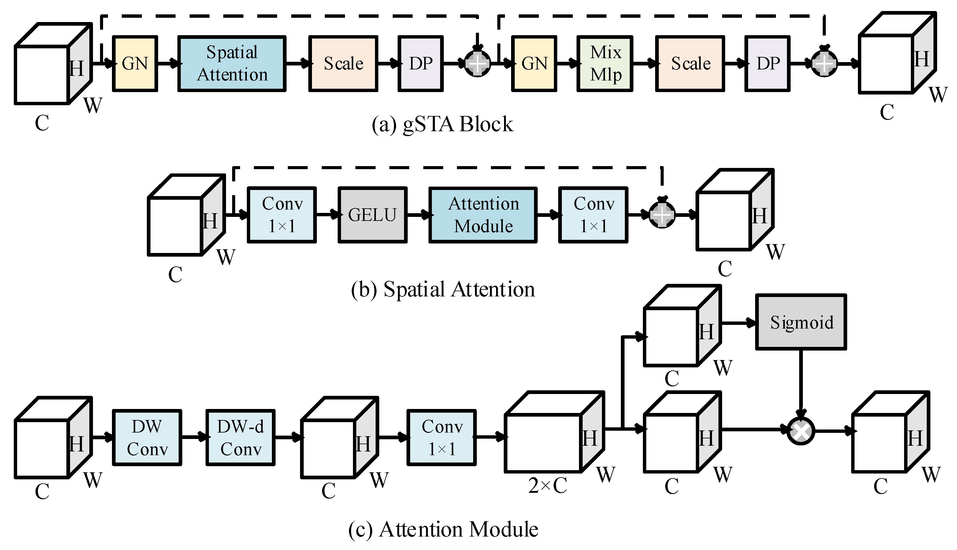
Figure 2.
Flowchart of the SimVPv2 model for SSH prediction. The batch dimension is omitted for clarity. The batch size is 40 (4 × 10) in both the Spatial Encoder and Spatial Decoder, and 4 in the Spatiotemporal Translator.
Figure 2.
Flowchart of the SimVPv2 model for SSH prediction. The batch dimension is omitted for clarity. The batch size is 40 (4 × 10) in both the Spatial Encoder and Spatial Decoder, and 4 in the Spatiotemporal Translator.
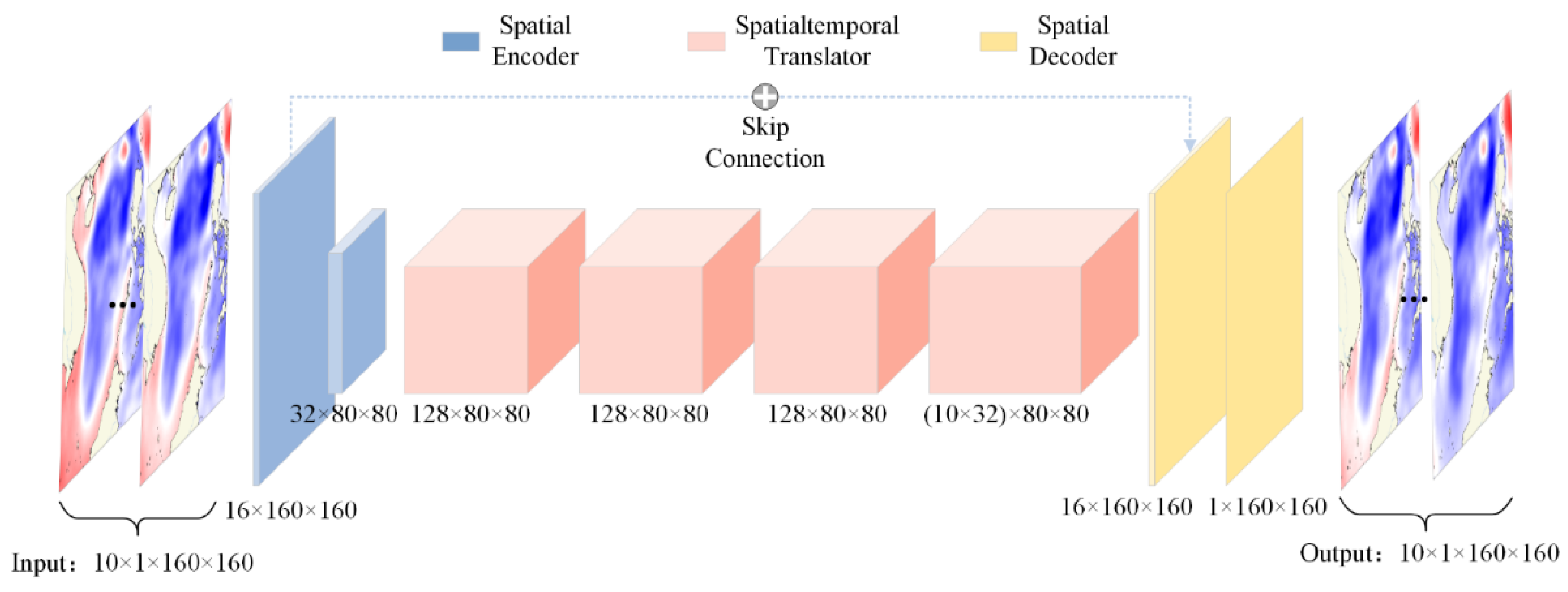
Figure 3.
(a) RMSE and (b) PCC between CMEMS target data and GCNNs predictions under different values of the geostrophic constraint coefficient λ. Dark blue dots represent the mean values from five models trained with identical configurations except random seeds; error bars indicate the 95% confidence intervals (CI) computed via Bootstrap method. Light blue points show individual results from each run. The Base (red dashed line) denotes the SimVPv2 model trained without applying any introduced strategies; the shaded region represents its 95% CI.
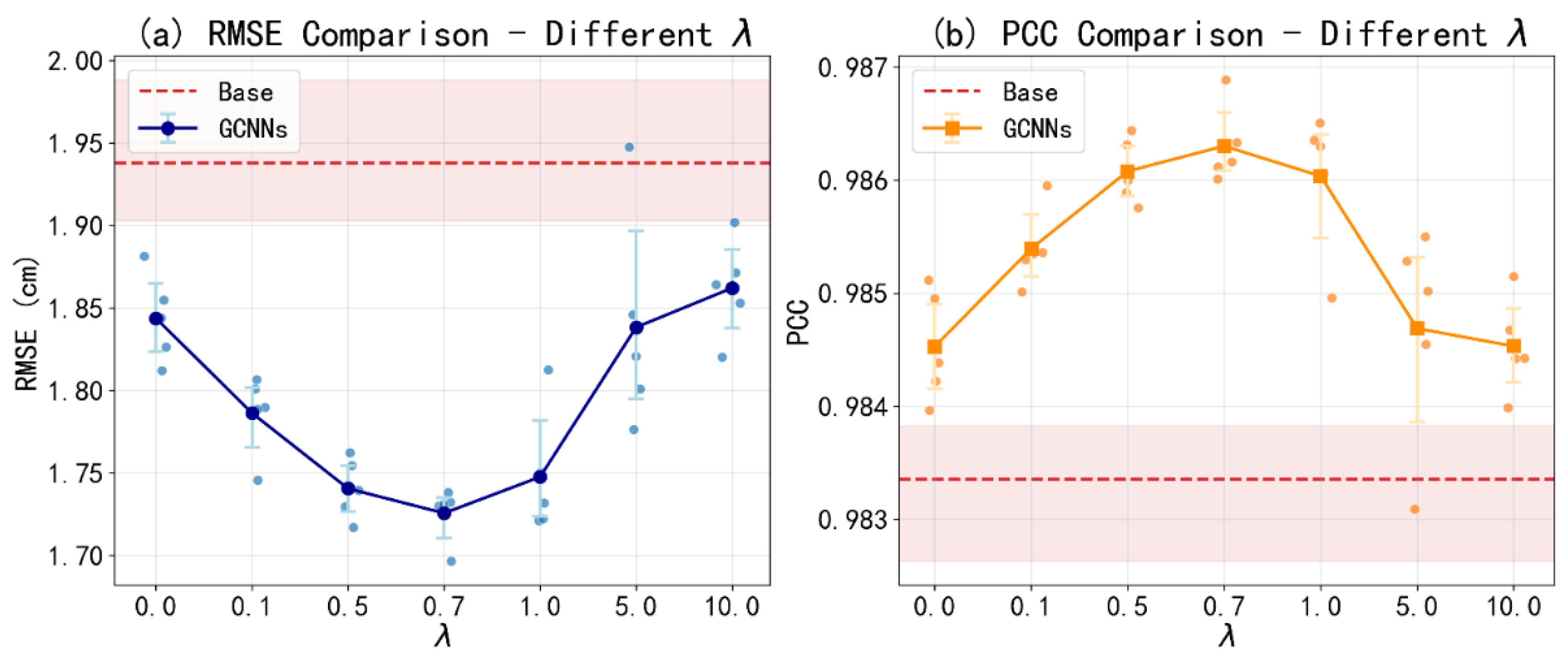
Figure 4.
Similar to Figure 3, except that the GCNN here specifically denotes the model incorporating all three strategies—geostrophic constraint (λ = 0.7), latitude-weighted loss, and mask-informed input—while “No GC”, “No LW”, and “No MI” correspond to models trained without the respective strategy.
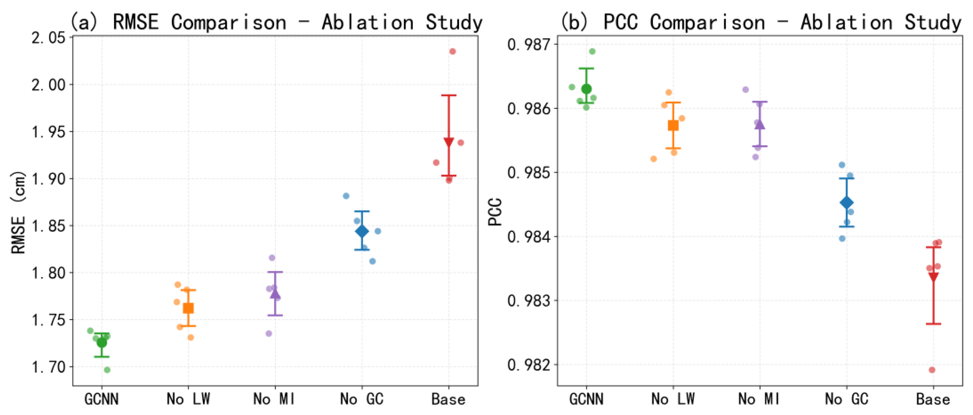
Figure 5.
Comparison of the forecast skill of different models at different lead time in the SCS from 1 January 2023 to 14 June 2024, using (a) RMSE and (b) PCC.
Figure 5.
Comparison of the forecast skill of different models at different lead time in the SCS from 1 January 2023 to 14 June 2024, using (a) RMSE and (b) PCC.
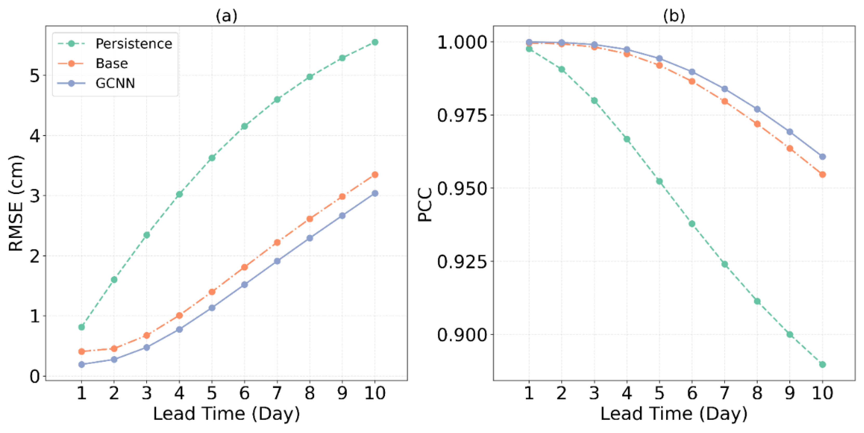
Figure 6.
(a) Lead-mean RMSE for the Base and the GCNN predictions versus date on the test dataset. Seasonal-mean (b) RMSE and (c) PCC at different forecast lead time, comparing performance of the Base and the GCNN.
Figure 6.
(a) Lead-mean RMSE for the Base and the GCNN predictions versus date on the test dataset. Seasonal-mean (b) RMSE and (c) PCC at different forecast lead time, comparing performance of the Base and the GCNN.
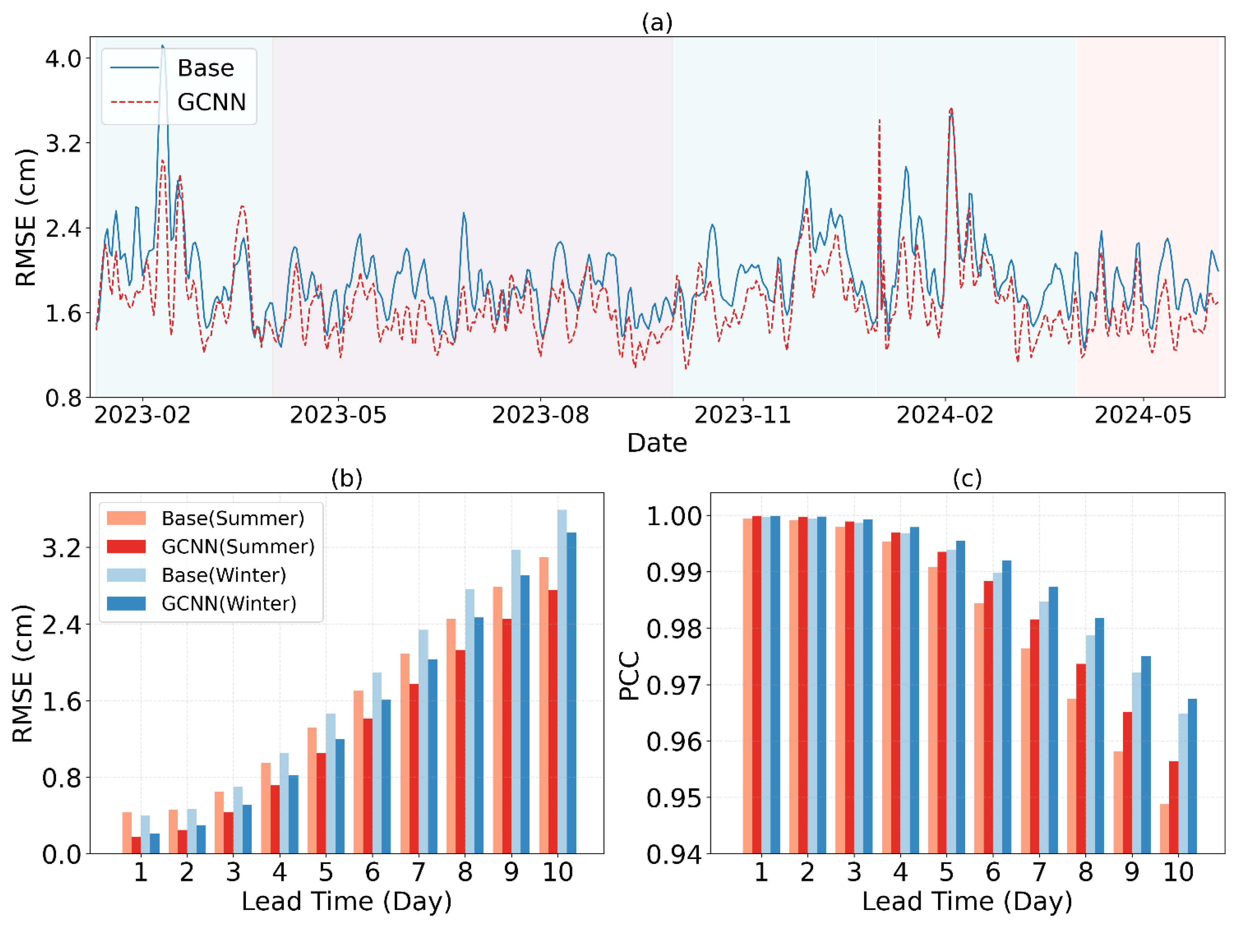
Figure 7.
The spatial distribution of the time-averaged prediction (a) absolute error (AE) for the Base model and (b) the absolute error reduction (AER) of the GCNN model compared to the Base model () from 1 January 2023 to 14 June 2024. The black line indicates the 200-meter isobath.
Figure 7.
The spatial distribution of the time-averaged prediction (a) absolute error (AE) for the Base model and (b) the absolute error reduction (AER) of the GCNN model compared to the Base model () from 1 January 2023 to 14 June 2024. The black line indicates the 200-meter isobath.
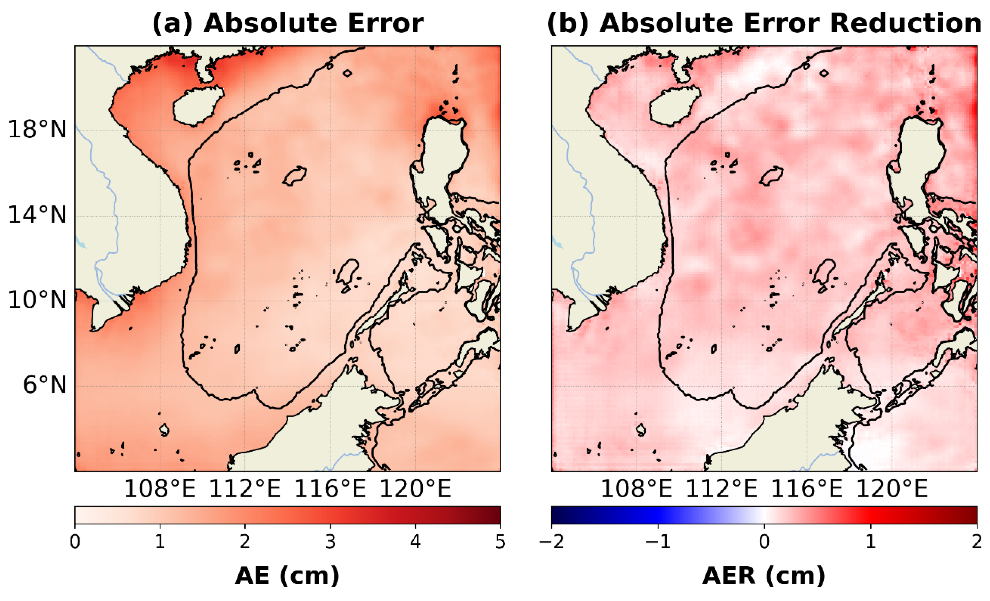
Figure 8.
Same as Figure 7, but for different lead times and seasons: (a) summer, (b) winter.
Figure 8.
Same as Figure 7, but for different lead times and seasons: (a) summer, (b) winter.
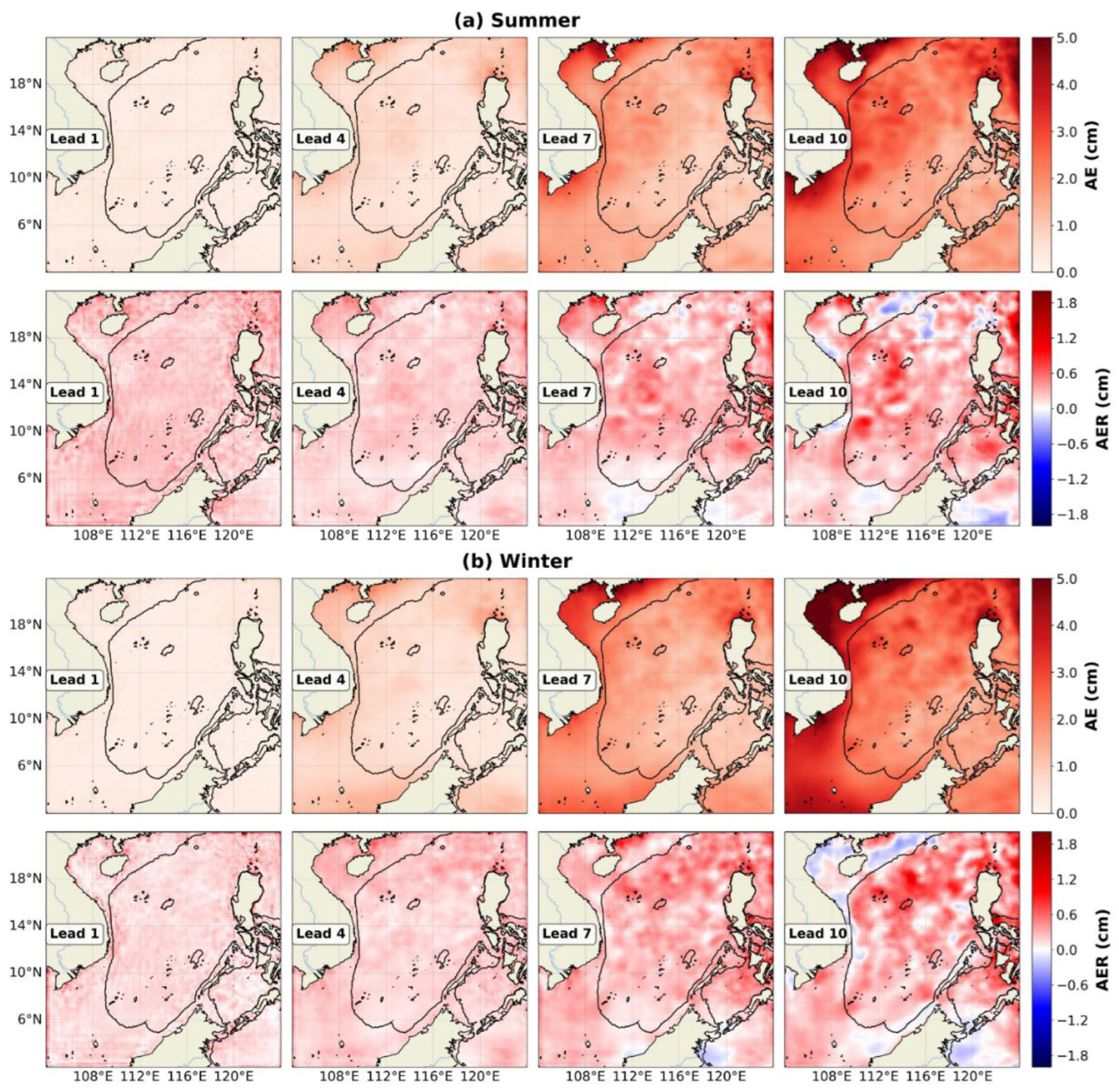

Table 1.
Independent replicate experiments using same random seeds.
| Model | RMSE (cm) | ||||
|---|---|---|---|---|---|
| Trial 1 | Trial 2 | Trial 3 | Mean | SD | |
| Base | 1.9768 | 1.9768 | 1.9768 | 1.9768 | 0 |
| Base + MI | 1.9329 | 1.9329 | 1.9329 | 1.9329 | 0 |
| Base + GC | 1.7899 | 1.7921 | 1.8242 | 1.8021 | 0.0157 |
| GCNN | 1.7309 | 1.7316 | 1.7286 | 1.7304 | 0.0013 |
Table 2.
Seasonal statistics of SSH variability and the PCC between and time-averaged absolute error (AE) of the Base prediction.
Table 2.
Seasonal statistics of SSH variability and the PCC between and time-averaged absolute error (AE) of the Base prediction.
| Season | (cm) | (cm) | PCC (100%) |
|---|---|---|---|
| Summer | 7.41 | 5.45 | 0.52 |
| Winter | 9.54 | 6.97 | 0.58 |
Table 3.
Model performance metrics (RMSE) for the whole domain (WD) and deep-basin areas (DB, depth > 200 m).
Table 3.
Model performance metrics (RMSE) for the whole domain (WD) and deep-basin areas (DB, depth > 200 m).
| Model | Scope | Full year | Summer | Winter |
|---|---|---|---|---|
| Base | WD | 1.977 | 1.851 | 2.096 |
| DB | 1.717 | 1.694 | 1.718 | |
| GCNN | WD | 1.732 | 1.593 | 1.876 |
| DB | 1.445 | 1.416 | 1.485 |
Disclaimer/Publisher’s Note: The statements, opinions and data contained in all publications are solely those of the individual author(s) and contributor(s) and not of MDPI and/or the editor(s). MDPI and/or the editor(s) disclaim responsibility for any injury to people or property resulting from any ideas, methods, instructions or products referred to in the content. |
© 2025 by the authors. Licensee MDPI, Basel, Switzerland. This article is an open access article distributed under the terms and conditions of the Creative Commons Attribution (CC BY) license (http://creativecommons.org/licenses/by/4.0/).
Copyright: This open access article is published under a Creative Commons CC BY 4.0 license, which permit the free download, distribution, and reuse, provided that the author and preprint are cited in any reuse.


