Submitted:
17 March 2025
Posted:
18 March 2025
You are already at the latest version
Abstract
Mesoscale eddies play a critical role in ocean circulation and biogeochemical processes, yet predicting their dynamic characteristics remains challenging due to nonlinear interactions and background errors in traditional methods. This study proposes a physics based Long Short-Term Memory (LSTM) network to predict key eddy features, amplitude, radius, and maximum circularly averaged speed (MCAs), by integrating multi-source observational data and hydrodynamic principles. Utilizing 28 years (1993-2020) of daily eddy trajectories from the global META3.1exp atlas and high-resolution reanalysis data (JCOPE2M) in the Northwest Pacific (15°-35°N, 115°-135°E), we systematically evaluate the effects of temporal sequence length and physical variables on prediction performance. The model demonstrates superior accuracy compared to conventional LSTM approaches, with mean absolute errors (MAE) for 1-7 day predictions increasing from 0.72 cm to 1.37 cm (amplitude), 8.85 km to 18.02 km (radius), and 0.80 cm/s to 2.46 cm/s (MCA). Key innovations include: 1) Dynamic reconstruction of spatiotemporal label-feature relationships to mitigate error accumulation, 2) Incorporation of sea surface temperature (SST) and height (SSH), which improve prediction accuracy by 5.33-5.92% and 3.65-5.47%, respectively, outperforming eddy kinetic energy inputs. Seasonal analysis reveals lower model accuracy in summer versus winter, particularly for amplitude (MAE: 1.29 cm vs 1.03 cm) and radius (15.3 km vs 13.2 km). Interannual error patterns correlate with El Niño events, highlighting climate-ocean coupling effects. This work advances eddy prediction through physics-guided machine learning, providing a framework for operational ocean forecasting. Future extensions could incorporate three-dimensional eddy structures and additional environmental drivers to enhance predictive capability.
Keywords:
mesoscale eddy
; LSTM networks
; eddy features prediction
; error analysis
1. Introduction
Mesoscale phenomena are ubiquitous and highly energetic features of ocean circulation [1].They carry enormous amounts of energy and have a significant impact on the transfer of mass, momentum and heat in the oceans, as well as on the distribution of organisms [2,3].Accurate prediction of the characteristics of mesoscale eddies can help us better understand the formation and evolution of ocean circulation and provide a scientific basis for the rational development of marine resources.
The study of mesoscale eddies has always been a hot area in marine science. With the continuous progress of observation technology, our understanding of mesoscale eddies has gradually deepened. From the early satellite remote sensing observation to the current multi-source data fusion, the research methods are constantly innovated. However, the prediction of mesoscale eddy characteristics still faces many challenges, such as the complex ocean environment, variable meteorological conditions and nonlinear dynamical processes. Generally, there are three main types of feature prediction methods for mesoscale eddies, namely, statistical prediction methods, numerical prediction methods, and machine learning prediction methods.
- (1)
- Statistical prediction methods build prediction models by analyzing historical data, Liu et al [4] developed a global eddy forecasting system, LICOM Forecast System, based on an ocean circulation model, was proposed to forecast the physical state of the ocean for 1-8 days. Robinson et al [5] originally used a mesoscale eddy observation network for predicting eddy evolution in two weeks, in which, the model is an anisotropic statistical model used for mixed spatio-temporal target analysis.
- (2)
- The numerical prediction method is based on the hydrodynamic equations, which are solved numerically to simulate the motion of the ocean and thus to predict mesoscale eddy features, Li et al [6] developed a multivariate linear regression model to predict eddy propagation trajectories at 1 - 4 weeks. This simple empirical model combines ocean parameters that mainly represent the beta effect and the mean flow advection with the position of eddy propagation. Xu et al [7] revealed the global distribution pattern of eddy variability by analyzing the overall pattern of spatial variations of the spectral slope of the wave number. With the development of computer technology, numerical forecasting has been applied to study ocean eddies. However, statistical prediction methods and numerical modeling methods have difficulties in predicting mesoscale eddy currents in terms of handling nonlinear features as well as background errors [8,9,10]. Machine learning (ML) methods appear to be effective in dealing with this aspect.
- (3)
- ML prediction methods have played an important role and achieved remarkable results in many fields of oceanography [11,12]. With the breakthroughs in satellite remote sensing technology, large-area and long-time series of ocean sample data can be obtained more easily, and the study of mesoscale eddy current has made many breakthroughs, especially in prediction method. Automatic identification and extraction of eddy current based on remote sensing data has become an effective means of predicting eddy current [13].Wang et al [14] constructed a prediction model for mesoscale eddy features and trajectories using a long and short-term memory network (LSTM) and extreme random trees. The root-mean-square errors (RMSE) between the predicted and actual longitudes (latitudes) of the trajectories range from 28.8 km to 47.2 km (23.8 km to 37.2 km). Ashkezari [15] used ML to predict the lifetime of vortices in steady evolution, constructed and extended a multivariate dataset of mesoscale eddy trajectories, and achieved a minimum centroid error of 8.507 km on 7-day prediction. Zhu et al [16] proposed a deep learning approach based on a video prediction model using a neural network to fuse remotely sensed meta-data with input data, which improved the accuracy with a prediction error of 5.6 km for 3-day prediction and 13.6 km for 7-day prediction of vorticity center position. Although ML algorithms are effective in predicting mesoscale eddy features, the forecasts are strongly affected by sea level anomalies noise in each grid, ignoring the internal physical relationships of eddy formation as well as the correspondence between before and after times. This is still a major challenge in predicting target eddies in current fields with complex physical fields remains.
To solve the above problems, this paper constructs a prediction model containing numerical vectors of the most relevant physical features of eddies based on mesoscale eddy properties and physical oceanographic theorems. The model uses an LSTM network to learn the spatio-temporal variation features to make comprehensive and accurate predictions of the target eddy currents at different prediction times. The important procedure are as follows: (1) Data preparation: Obtain mesoscale eddy data from the global atlas and sea surface data from JCOPE2M, and calculate related physical quantities for model input, (2) Model training: Utilize the LSTM network with its unique gate mechanism to train on the processed data to form an integrated learning system for predicting eddy features, and (3) Result evaluation: Employ MAE and RMSE to assess the model's performance on 63630 eddy samples over 1-7 days, and analyze the impacts of different factors on prediction errors.
The experimental results show that the performance of the proposed method is superior to that of previously studied methods. The prediction of eddy current properties relies more on historical time series data than on propagation trajectories. Finally, the variability characteristics and predictability of eddy current properties and propagation trajectories are discussed. The eddy properties have different effects on the model performance in propagation prediction.
2. Data and Methodology
In this paper, we predicted the eddy characteristics and analyzed the propagation characteristics based on 28 years (1993-2020) of daily mesoscale eddy signature data, using 15°-35°N latitude and 115°-135°E longitude as the test area. The overall process framework is shown in Section 2.2. The characterization factors can be divided into two categories. One category describes the relevant characteristics of the eddy itself, including amplitude (Amp), radius (Rad) and maximum circularly averaged (MCA) speed. These characteristics reflect the real state of eddies on the two-dimensional sea surface. The other involves the spatio-temporal information and physical factors related to the changes of the above eddy features, eddy latitude (Lon) and longitude (Lat), eddy kinetic energy(EKE), sea surface temperature (SST), sea surface height (SSH), and so on. During the evolution of eddies, the properties and propagation trajectories are dynamically changing and interrelated. The two-dimensional properties of eddies are related to the motion and reflect the current state and changes of the eddies.
2.1.1. Mesoscale Eddy Data
This paper uses the global mesoscale eddy track atlas (META3.1exp DT) published by Cori Pegliasco et al [17], which is available in the Archiving, Validation and Interpretation of Satellite Oceanographic Data (AVISO) (https://www.aviso.altimetry.fr/en/data/data-access). The track atlas consists of trajectories generated from eddy identification and altimetry maps, and the resolved detection method used is derived from the py-eddy-tracker (PET) algorithm developed by Mason et al. [18], which is an improvement on the earlier META2.0, providing complementary eddy information such as eddy shapes, eddy fringes, maximum speed contours, and average eddy speed from centre to edge profiles. The multi-physical information helps the mechanical learning algorithm to improve its accuracy [19], therefore, it is selected in this paper as a source of mesoscale eddy features.
2.1.2. Sea Surface Physical Information Data
The high-resolution reanalysis dataset used for the physical information is derived from the Japan Coastal Ocean Predictability Experiment (JCOPE2M) dataset released by the Japan Agency for Marine-Earth Science and Technology (JAMSTEC), which can be accessed at http://www.jamstec.go.jp/jcope/ [20]. JCOPE2M covers the western North Pacific Ocean with a temporal resolution of 1 day and a horizontal resolution of 1/12°. It is widely used to study mesoscale phenomena and flow fields by assimilating high-resolution satellite sea surface temperature (SST) data, sea surface altitude (SST) level data, and in-situ data into the model using a multiscale three-dimensional variational method [21].
2.2. LSTM Network for Eddy Current Feature Prediction
LSTM is a special type of recurrent neural network, proposed by Hochreiter and Schmidhuber in 1997 [22]. It is designed to solve the problems of gradient vanishing and gradient explosion encountered by traditional recurrent neural network(RNN) when dealing with long sequence data, and to maintain the persistence of information in the loaded sequence data [23,24]. In this paper, an attempt is made to use LSTM neural network to train the prediction of mesoscale eddy feature sequences under different labeled sequences. The ability of LSTM network to deal with the long and short-term dependencies can be effectively improved with the existence of mesoscale eddy sequences under the META3.1 dataset with time series spanning from tens to thousands. The key of the LSTM is its special network structure, by which, we can predict eddy feature sequences under different labeled sequences through the introduction of the structure which controls the inflow, storage and outflow of information by introducing a gating mechanism [25]. As shown in Figure 1, the LSTM network is a cell form, which is consisted of three gates. And the strcuture of these gates are descrebed as followed.
- (1)
- Forgeting Gate (FG): FG determines to forget or retain information from the cell. And, FG consists of a sigmoid layer that determines which historical information should be discarded from the cell. The processed data will produce the state of the neural unit at a specific point in time, and this state is continuously transmitted over the time series. When the neural unit receives a new input, it is updated by combining the current input value with the output value from the previous point in time. The input information passes through the FG,and the forgetting functions is
Where is a vector input at moment t, is an output of the previous moment; is a weight matrix corresponding to the current calculation, is the bias corresponding to the current computation, is the state of the neural unit at the previous moment, is the sigmoid function, is the product of the corresponding elements, is the Physical information data at the current moment.
According to (1), we determine what information is unnecessary and should be deleted from memory.
- (2)
- Inputing Gate(IG): IG determines which information enters the cell from the input x. It is a sigmoid layer and a tanh layer. It consists of two sigmoid layers and a tanh layer. The prior sigmoid layer decides inputing values it, which is given by
Where 、、denote the weight matrix corresponding to the current computation, respectively. is bias matrix.
The next sigmoid layer together with the tanh layer decides the new value of the cell, which is
Where 、、denote the weight matrix and bias corresponding to the current computation, respectively.
After through FG and IG, we get the cell state value , is written by (4), and taken as the inputing value of the naxt update cell.
- (3)
- Outputing Gate(OG): OG determines what information is output from the cell state. It also consists of two sigmoid layers. The first sigmoid layer decides which information will be output from the cell state to the next hidden state, and the second sigmoid layer together with the tanh layer decides the next hidden state of the cell state.
The output arithmetic process of the neural cell at the current moment is
Where , is an output of the OG.、、denote the weight matrix corresponding to the current computation, respectively. is a bias matrix.
In this paper, LSTM networks are used to predict eddy properties. Mesoscale eddy motion (including speed, shape, radius, displacement, etc.) is a process with temporal and spatial variations [26]. During the motion process, the positions and properties of vortices at different moments are characterized, and these properties are related to the previous motion state. Therefore, the future state of mesoscale eddies can be predicted from the parameters characterizing multiple moments in the previous sequence. vortices at time t are considered as the inputing values of the LSTM model.The time series forecasting model can be represented as follows
Under the time-series model, we consider a machine learning model based on the corresponding relationships ((X,t),(Y,t+n)) in the eigenvectors (x,t) and the predicted values (Y,t+n) at different prediction time steps n, and we constructed a machine learning model to explore the implicit relationship between these eigen factors and the eddy current prediction labels. The prediction algorithm consists of the following steps.
Step 1: Process all mesoscale eddy data within the experimental sea area, and rearrange the individual eddy feature data Xn containing the complete time series into a new sequence according to eddy labels and before and after time after clearing the missing values and outliers.
Step 2: The eddy feature X at time t is combined with the predicted value Y under the same eddy label at time t+1 to form a correspondence ((X,t), (Y,t+n)), which is preprocessed and inputted into the model to obtain the three prediction models for eddy amplitude, radius and MCAs.
Step 3: According to the longitude and latitude and the time difference before and after in the eddy characteristics, the meridional velocities () and latitudinal velocities () are obtained in accordance with (7) and (8), and the meridional and latitudinal velocities are brought in to generate the EKE in accordance with (9).
Where is the fluid density, which is looked on as a constant value in the surface of the experimental sea area.
Step 4: Input the data Xm such as EKE, sea surface temperature, sea surface height, etc. into the model also according to the step 1 and step 2 to get the eddy feature input based on physical information.
Step 5: Repeat the above steps according to the prediction time interval of n. Then independent model matrices for different prediction objectives are obtained and the training models are parallelized to form an integrated learning system for eddy current feature prediction.
The overall process framework is shown in Figure 2.
3. Experiment and Results
3.1. Evaluation Criteria
In our model, training starts with initializing the weights of the interlayer nodes and updating the parameters by gradient descent. According to the iterative processing of the training set, the loss function is minimized to obtain the optimal solution [27,28], while the model predictions are assimilated using the true values at regular intervals to further improve the accuracy of the model predictions.
In order to evaluate the performance of the model in predicting mesoscale eddy currents, the mean absolute error (MAE) and RMSE are used as the criteria to judge the performance of the prediction model [29]. The formulae for each evaluation error index are shown in (10) and (11), repectively.
Where is the predicted values obtained after model training, is observed true values and n is the number of samples. The smaller the values of MAE and RMSE obtained, the superior the performance of the model.
3.2. Prediction of Mesoscale Eddy
Mesoscale oceanic eddies reserve a huge amount of energy and play an important role in material and energy transport and air-sea interaction [30,31,32,33]. In this study, we obtain a large number of valid samples based on eddy position and property information recorded in the eddy track dataset, and used machine learning to investigate the eddy evolution trend. Figure 3 shows the histogram of the property information, including amplitude, radius and MCA information, for the study sea area from 1993 to 2020; the mean values of the three properties about amplitude, radius, and average speed are 3.83 cm, 59.57 km, and 20.74 cm/s, respectively.
The development of mesoscale eddies is often accompanied by oblique pressure instability, which makes mesoscale forecasts particularly sensitive to initial conditions [34,35]. At the same time daily variations in eddy current characteristics are usually stable and small. However, as the prediction time increases, the stability of this variation decreases. The model can learn complex trends by using feature information and variations from previous time steps, and the gate structure of the LSTM network can be used to transmit and update important features in the historical information time series, as well as to selectively forget invalid information. Historical time series, which are too long, are wasteful of resources and require long run times, therefore, such series are not suitable for sample testing or processing of missing data. In the prediction of eddy current properties, we use historical datasets with different time series lengths to train and test the performance of the LSTM model. In eddy radius prediction, the model gets the best performance when the prediction time is short and the time series length is 5 days. When the prediction time is relatively long, a time series length of 7 days leads to the lowest prediction error. For eddy amplitude and MCA prediction, the prediction results are similar for different time series lengths, which indicates that the time series length has little effect on the model performance. It is worth nothing that the prediction error of the model is so small that small changes in the time series length are not reflected in the overall index.
We calculated the prediction results for 63630 eddy current samples using the optimal parameters of the LSTM model. Figure 4, Figure 5, and Figure 6 show the temporal distribution of the errors in eddy current properties over the 1-7 day prediction time. As the prediction time increases, the number of eddies with large absolute errors increases and the number of eddies with small errors decreases, resulting in an increase in the average absolute error for all tested eddies. The distribution of errors of eddy properties is also related to their absolute values, with eddies characterized by smaller properties producing relatively small errors. Table 1 lists the MAEs of eddy properties for different prediction times and compares recent studies on eddy prediction. Ma et al [8] found that the polarity of eddy currents has little effect on the prediction of eddy characteristics, so instead of distinguishing between eddy polarity, we use the average of the prediction errors of cyclonic and anticyclonic eddies obtained by Ma et al. as the measurement standard for the model in this paper.
The results show that the prediction accuracy of the model decreases with the increase of the number of prediction days, and the MAE increases continuously, and the MAE of the mesoscale eddy amplitude prediction in the study sea area gradually increases from 0.72 cm on the first day of the forecast to 1.37 cm on the seventh day, the MAE of the radius prediction increases from 8.85 km to 18.02 km on the first day, and the MAE of the MCAs prediction increases from 0.80 cm/s to 2.46 km/s. The results indicate the superiority of the proposed model in this paper, which is much better than the LSTM network model proposed by wang et al. in terms of prediction accuracy, and the results also indicate the efficiency of the model in this paper in predicting mesoscale eddy properties and its ability to address the shortcomings of traditional prediction methods. We try to rebuild the correspondence between the spatio-temporal labels in the dataset and the mesoscale eddy features after each training of the network, which effectively prevents the model from accumulating errors during the training, and makes each prediction relatively independent, which is reflected in the smooth increase of the 7-day prediction error.
4. Discussion
In the study, we build an LSTM network for mesoscale eddy feature prediction based on physical information under the LSTM network, and try multiple factors including EKE, spatio-temporal information, sea surface temperature, sea surface height and other factors are added to the network for training, and according to the conclusions of Xu et al [18], the appropriate input of physical information can lead to the improvement of the model prediction accuracy of the network after training by 2.80% to 11.92% .In order to verify that these physical factors do play an important role in the prediction model, this paper also tries to analyse the error of the model prediction of mesoscale eddy features under the initial conditions by adding EKE, sea surface temperature, sea surface height, etc. and adjusting them to the best network parameters. The training results are shown in Figure 8.
We attempted to train the model 42 times for each of the four physical information input types when all other things being equal, to obtain the results of the box-and-line plot above, where the mean RMSE values of the model's predictions of the mesoscale eddy's 7-day amplitude, radius, and MCAs under the initial conditions are 1.69 cm, 19.2 km, and 2.56 cm/s, respectively. When EKE is added to the model, the mean RMSE values of the three features are 1.68 cm, 19.2 km and 2.55 cm/s, respectively, while adding sea surface temperature to the model, the mean RMSE values of the three features are 1.60 cm, 18.6 km and 2.45 cm/s, respectively, while adding sea surface height to the model, the mean RMSE values of the three features are 1.59 cm, 18.5km and 2.42 cm /respectively. The results show that the EKE has a limited, or perhaps even non-existent improvement on the model performance when other parameters are kept constant, which we speculate, is because the EKE itself is derived from the latitude/longitude and spatial/temporal information of the eddy trajectory atlas according to the formulae. Essentially, there is no optimisation of the model training without new information inputting. While adding the sea-surface temperature to the model, the mesoscale eddy 7-day amplitude, radius, and MCAs are improved by 5.33%, 3.13%, and 4.30%, respectively. After adding sea surface height, the prediction accuracies of the three features are improved by 5.92%, 3.65%, and 5.47%, respectively. Therefore, we conclude that the significant enhancement of model prediction performance, by the addition of sea surface temperature and sea surface height, is attributed to the input of new physical information. At the same time, this physical information is independent of the original dataset, which is equivalent to enhancing the input dimension of the original model and increasing the information abundance. This result also shows that sea surface temperature play an important role in the variation of mesoscale eddy features as well as sea surface height.
In addition to the above results, we also discuss the interannual variability of mesoscale eddy features, and obtain the predicted RMSEs for the amplitude, radius, and MCAs of mesoscale eddies in different years and different seasons, respectively, and the results are shown in Figure 9.
Comparing the RMSEs of the three features in different years with the average RMSE, we find that there seems to be some kind of overlap in the prediction accuracy of the three features, namely, almost all of them have a low prediction accuracy in the years of 1993-1994, 1997-1998, 2004-2005, 2009-2010, 2014-2016, and 2020-2021, while, a high or unstable prediction accuracy in the rest of the years. We consider that the above pheonomenon is related to the El Niño events. Furthermore find that the years above-mentioned are El Niño years.
In terms of seasonal differences, the MAEs of the three features of the mesoscale eddies in the summer and winter seasons are statistically calculated, and the results in Table 2 show that the differences between the summer and winter seasons do not seem to be reflected in the speed of the MCAs, whereas there are more obvious differences in the amplitude and radius.
Various studies in recent years have pointed out that eddy motion is correlated with topography, season, and various other physical quantities [36,37]. In this paper, an end-to-end approach is used to directly establish the correlation between the initial characteristics of eddies and their propagation trajectories. Although more important and complex changes may occur, eddy characteristics are a direct result of speed variations and other influences that include recent eddy propagation patterns influenced by beta effects and mean advection [13]. Since the complexity of eddy motion is the result of a combination of factors, training based on machine learning algorithms can indirectly reflect the correlation of other factors affecting eddy propagation trajectories, thus effectively enabling the prediction of eddy trajectories.
5. Conclusions
This study developed a LSTM-based model incorporating physical information for mesoscale eddy characteristic prediction. Using data from the global mesoscale eddy trajectory atlas and JCOPE2M dataset within the specified test area (15°-35°N, 115°-135°E) from 1993 - 2020, the experiment result demonstrate the proposed model has the more accuracy performance than that of the conventional models.
In the prediction of eddy amplitude, radius, and MCA speed, the MAE values increased with the extension of the prediction time from 1 to 7 days. For instance, the MAE of amplitude rose from 0.72 cm to 1.37 cm. The model outperformed previous LSTM models in accuracy. By reconstructing the correspondent relationship between samples and labels, avoiding error accumulation effectively, and ensuring the reliability of the prediction results. Although EKE had a negligible effect on model improvement, sea surface temperature and sea surface height, compared to the rest proposed information, significantly enhanced the prediction accuracy of the three eddy characteristics by different percentages.
In the analysis of interannual variability, a potential relationship between prediction errors and the El Niño phenomenon was identified. In addition, there were obvious seasonal differences in the prediction accuracy of eddy amplitude and radius. We got the lower accuracy in summer, conversely, the higher accuracy in winter.
It should be noted that the analyses and methods provided in this paper need to be further refined and deepened, and the prediction of individual mesoscale eddy characteristics, intensity and size, especially the seasonal differences in mesoscale eddy systems, need to be further evaluated. Future research may focus on integrating more variables, such as solar cycle, tidal and currents, to further enhance the model's performance and deepen the understanding of mesoscale eddy behavior. In addition, due to the lack of suitable observations, this paper focuses only on the two-dimensional structure of mesoscale eddies, the three-dimensional field structure is not discussed in this paper, and this element will be carried out in a subsequent study.
Author Contributions
W.Z. and X.W. conceived and designed the experiments; W.Z. performed the experiments and wrote the paper; X.W. helped with field work, discussion, and revisions. All authors have read and agreed to the published version of the manuscript.
Funding
This research was funded by the National Science Foundation of China (61071006).
Acknowledgments
All the data used in this study are available as follows: The global mesoscale eddy track atlas is from the Archiving, Validation and Interpretation of Satellite Oceanographic Data (AVISO) (https://www.aviso.altimetry.fr/en/data/data-access), and the Japan Coastal Ocean Predictability Experiment (JCOPE2M) dataset is from the Japan Agency for Marine-Earth Science and Technology (JAMSTEC) (http://www.jamstec.go.jp/jcope/).
Conflicts of Interest
The authors declare no conflict of interest.
References
- McGillicuddy,J D. Mechanisms of Physical-Biological-Biogeochemical Interaction at the Oceanic Mesoscale. J. Annual Review of Marine Science,2016,8(1), 125-159.
- Zhu, Y.; Peng, S. A vortex-implanted initialization scheme for the mesoscale eddy prediction: Real simulation and hindcast. J. Ocean Modelling,2025,194, 102489-102489.
- Ma, X.; Zhang, L.; Xu, W. AB-LSTM: a mesoscale eddy feature prediction method based on an improved Conv-LSTM model. J. Frontiers in Marine Science, 2024, 11, 1463531–1463531. [Google Scholar]
- Hailong, L.; Pengfei, L.; Weipeng,Z. A global eddy-resolving ocean forecast system in China – LICOM Forecast System (LFS). J. Journal of Operational Oceanography, 2023, 16(1), 15-27.
- Ashkezari, M.D.; Hill, C.N.; Follett, C.N.; Forget, G.; Follows, M.J. Oceanic eddy detection and lifetime forecast using machine learning methods. Geophys. Res. Lett. 2016, 43, 12234–12241. [Google Scholar]
- Li, J.; Wang, G.; Xue, H.; Wang, H. A simple predictive model for the eddy propagation trajectory in the northern South China Sea. Ocean Sci. 2019, 15(3), 401–412. [Google Scholar]
- Xu, Y.; Fu. Global Variability of the Wavenumber Spectrum of Oceanic Mesoscale Turbulence. J. Journal of Physical Oceanography, 2011, 41(4), 802-809.
- Li, J.; Wang, G.; Xue, H.; Wang, H. A simple predictive model for the eddy propagation trajectory in the northern South China Sea. Ocean Sci. 2019, 15, 401–412. [Google Scholar]
- Ma, C.; Li, S.; Wang, A.; Yang, J.; Chen, G. Altimeter Observation-Based Eddy Nowcasting Using an Improved Conv-LSTM Network. Remote Sens. 2019, 11(12), 783. [Google Scholar] [CrossRef]
- W.; Huizan, W.; Donghan, L. The Prediction of Oceanic Mesoscale Eddy Properties and Propagation Trajectories Based on Machine Learning. J. Water, 2020, 12(9), 2521-2521.
- Doan, V.-S.; Huynh-The, T.; Kim, D.-S. . Underwater acoustic target classification based on dense convolutional neural network. IEEE Geosci. Remote Sens. Lett. 2020, 19, 1–5. [Google Scholar]
- Yang, H.; Zhu, R.; Chen, Z.; Li,J.; Wu, L. Temperature Variability and Eddy‐Flow Interaction in the South of Oyashio Extension. J. Journal of Geophysical Research: Oceans, 2022, 127(11).
- Duo, Z.; Wang, W.; Wang, H. Oceanic Mesoscale Eddy Detection Method Based on Deep Learning. Remote Sens. 2019, 11, 1921. [Google Scholar] [CrossRef]
- Wang, X.; Wang, H.; Liu, D.; Wang, W. The prediction of oceanic mesoscale eddy properties and propagation trajectories based on machine learning. Water, 2020, 12, 2521. [Google Scholar] [CrossRef]
- Ashkezari, M.D.; Hill, C.N.; Follett, C.N.; Forget, G.; Follows, M.J. Oceanic eddy detection and lifetime forecast using machine learning methods. Geophys. Res. Lett. 2016, 43, 12234–12241. [Google Scholar] [CrossRef]
- Zhu, R,; Song, B.; Qiu, Z,; Yuan, T. A Metadata-Enhanced Deep Learning Method for Sea Surface Height and Mesoscale Eddy Prediction. J. Remote Sensing, 2024, 16(8), 1466-1491.
- Cori, P.; Antoine, D.; Evan, M.;Morrow, R.; Faugère, Y. META3.1exp: a new global mesoscale eddy trajectory atlas derived from altimetry. J. Earth System Science Data, 2022, 14(3), 1087-1107.
- Mason, E.; Pascual, A.; McWilliams, J.C. A New Sea Surface Height–Based Code for Oceanic Mesoscale Eddy Tracking. J. Atmos. Ocean. Technol, 2014, 31, 1181–1188. [Google Scholar] [CrossRef]
- Xu, W.; Zhang, L.; Li, M.; Ma, X.; Wang, H. A physics-informed machine learning approach for predicting acoustic convergence zone features from limited mesoscale eddy data. J. Frontiers in Marine Science, Mar. Sci. 11, 1364884.
- Ohishi, S. , Miyoshi, T. & Kachi, M. LORA: a local ensemble transform Kalman filter-based ocean research analysis. Ocean Dynamics, 2023, 73, 117–143. [Google Scholar]
- Ocean Research, Recent Research from Institute of Oceanography 2 Highlight Findings in Ocean Research (Tempo-spatial Variations of the Kuroshio Current In the Tokara Strait Based On Long-term Ferryboat Adcp Data). J. Energy & Ecology, 2019.
- Eduardo, M.; Yassine, B.; João, M. KDBI special issue: Explainability feature selection framework application for LSTM multivariate time-series forecast self optimization. J. Expert Systems, 2024, 42(2), 13674-13674.
- Zhang, Q.; Wang, H.; DONG, J. Prediction of Sea Surface Temperature using Long Short-Term Memory. J. IEEE Geoscience and Remote Sensing Letters, 2017, 14(10), 1745-1749.
- SONG, G.; PENG, Z.; BIN, P.; Yaru,L.; Min, Z. A nowcasting model for the prediction of typhoon tracks based on a long short term memory neural network. J. Acta Oceanologica Sinica, 2018, 37(05), 8-12.
- Pankaj, C.; Muhammed, E.; Rajib, S.; Kalachand, S. Forecast future disasters using hydro-meteorological datasets in the Yamuna river basin, Western Himalaya: Using Markov Chain and LSTM approaches. J. Artificial Intelligence in Geosciences. 2024, 5, 100069. [Google Scholar]
- Chen, Y.; Zhao, Z.; Yang, Y.; Li, X.; Peng, Y.; Wu, H.; Zhou, X.; Zhang, D.; Wei, H. BiST-SA-LSTM: A Deep Learning Framework for End-to-End Prediction of Mesoscale Eddy Distribution in Ocean. J. Journal of Marine Science and Engineering, 2024, 13(1), 52.
- Zhang, K.; Chao, W.-L.; Sha, F.; Grauman, K. Video Summarization with Long Short-Term Memory. In Proceedings of the 14th European Conference on Computer Vision (ECCV), Amsterdam, The Netherlands, 11–14 October 2016; pp. 766–782. [Google Scholar]
- Wang, D.; Su, J.; Yu, H. Feature Extraction and Analysis of Natural Language Processing for Deep Learning English Language. IEEE Access 2020, 8, 46335–46345. [Google Scholar]
- Ma, X.; Zhang, L.; Xu, W.; Li, Q.; Li, M. Analysis and prediction of mesoscale eddy kinetic energy variations in the Kuroshio extension. J. Dynamics of Atmospheres and Oceans, 2024, 108, 101497–101497. [Google Scholar]
- Dong, D.; Brandt, D.; Chang, P.; et al. 2017. Mesoscale eddies in thenorthwestern Pacific Ocean: Three-dimensional eddy struc-tures and heat/salt transports. J. Geophysical Re-search, Oceans, 122(12), 9795–9813.
- Sun, B.; Liu, C.; Wang, F. 2019b. Global meridional eddyheat transport inferred from Argo and altimetry observations. J. Scientific Reports, 9(1), 1345.
- Sun, B.; Xu, S.; Wang, Z.Spatiotemporal features and vertical structures of four types of mesoscale eddies in the Kuroshio Extension region. J.Acta Oceanologica Sinica,2024,43(05):30-40.
- Yang, G.; Zheng, Q.; Xiong, X. 2023. Subthermo-cline eddies carrying the Indonesian Throughflow water ob-served in the southeastern tropical Indian Ocean. J. Acta Oceano-logica Sinica, 42(5), 1–13.
- Li, Z.; Fei, J.; Zhang, R.; et al. Numerical prediction of oceanic mesoscale circulation and satellite altimetry data assimilation in the Western Pacific. J. Sci. China Earth Sci, 2025, 68, 909–927. [Google Scholar]
- McWilliams, J. Submesoscale currents in the ocean. Proc R Soc A, 2016, 472, 20160117. [Google Scholar] [PubMed]
- Nan, F.; Xue, H.; Yu, F. Kuroshio intrusion into the South China Sea: A review. Prog. Oceanogr. 2015, 137, 314–333. [Google Scholar]
- Du, Y.; Wu, D.; Liang, F.; Yi, J.; Mo, Y.; He, Z.; Pei, T. Major migration corridors of mesoscale ocean eddies in the South China Sea from 1992 to 2012. J. Mar. Syst. 2016, 158, 173–181. [Google Scholar]
Figure 1.
Structure of LSTM network based on physical features.
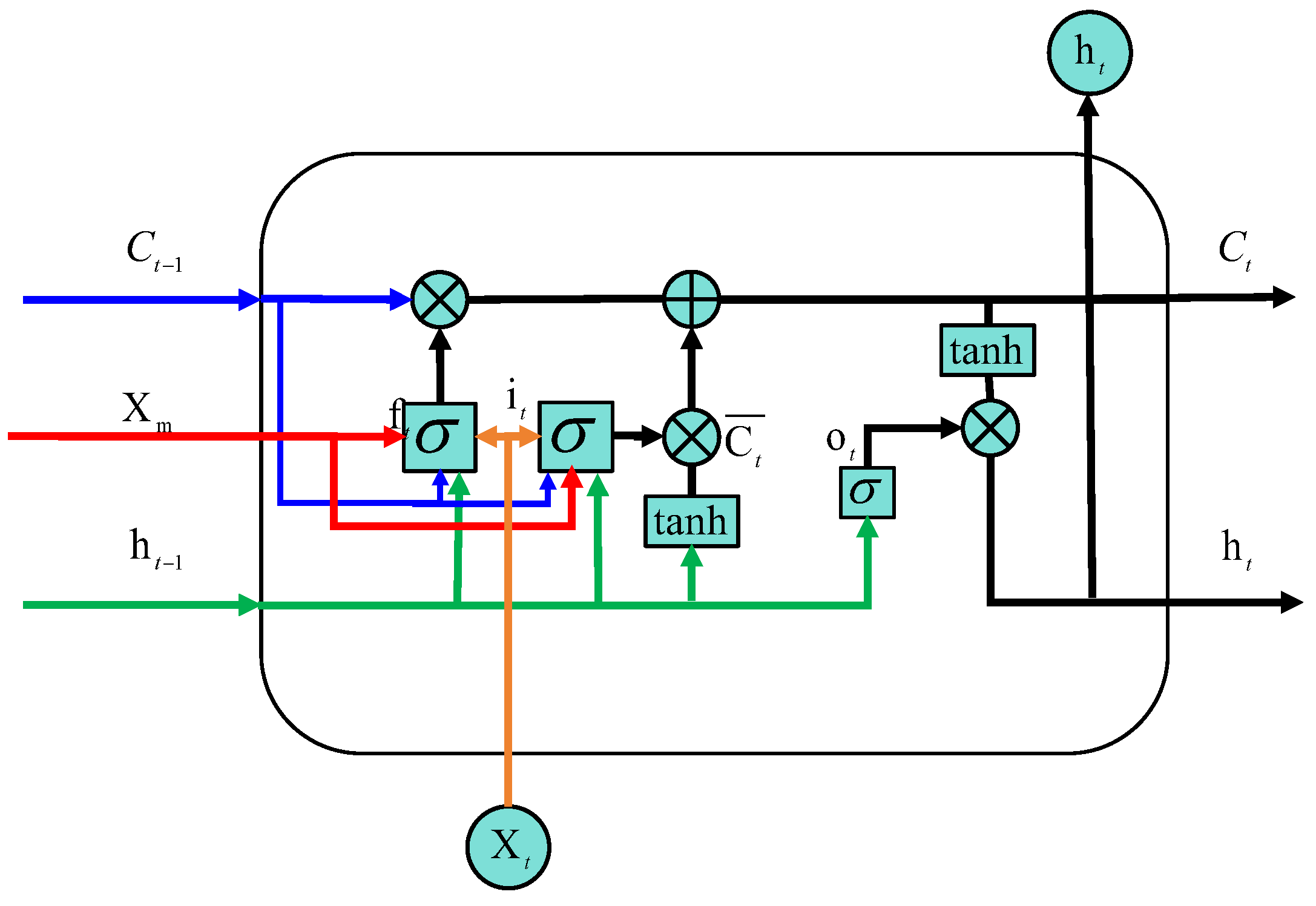
Figure 2.
Framework for predictive analysis of eddy current properties.
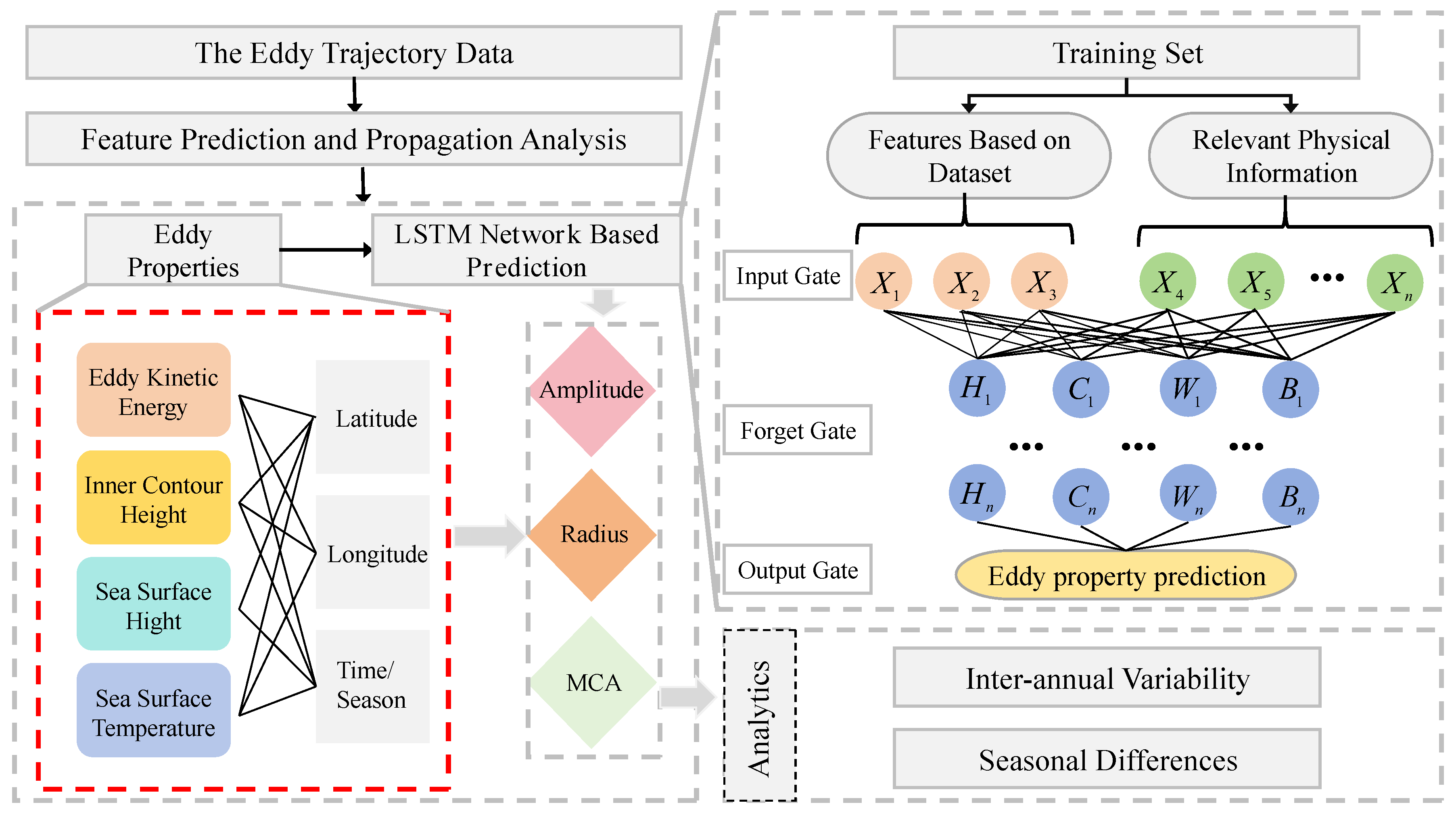
Figure 3.
Histogram of eddy current characteristics from 1993 to 2020.
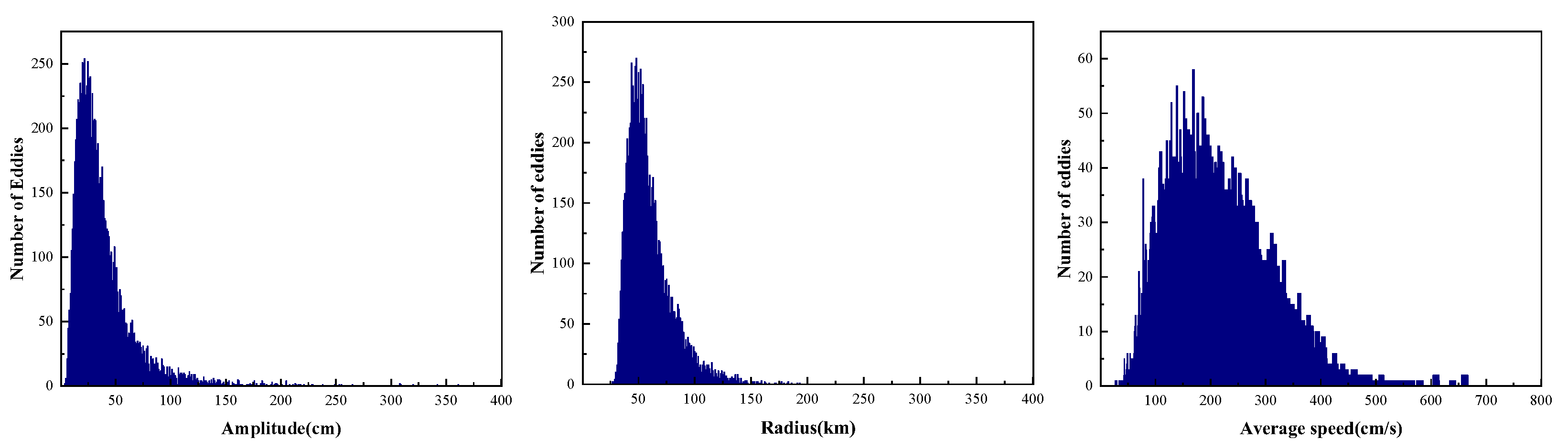
Figure 4.
(a) Scatterplot of the spatial distribution of eddy amplitudes (cm) in the test set. And Figure 4 (b-h) Forecast errors (cm) of eddy amplitudes from day 1 to day 7.
Figure 4.
(a) Scatterplot of the spatial distribution of eddy amplitudes (cm) in the test set. And Figure 4 (b-h) Forecast errors (cm) of eddy amplitudes from day 1 to day 7.
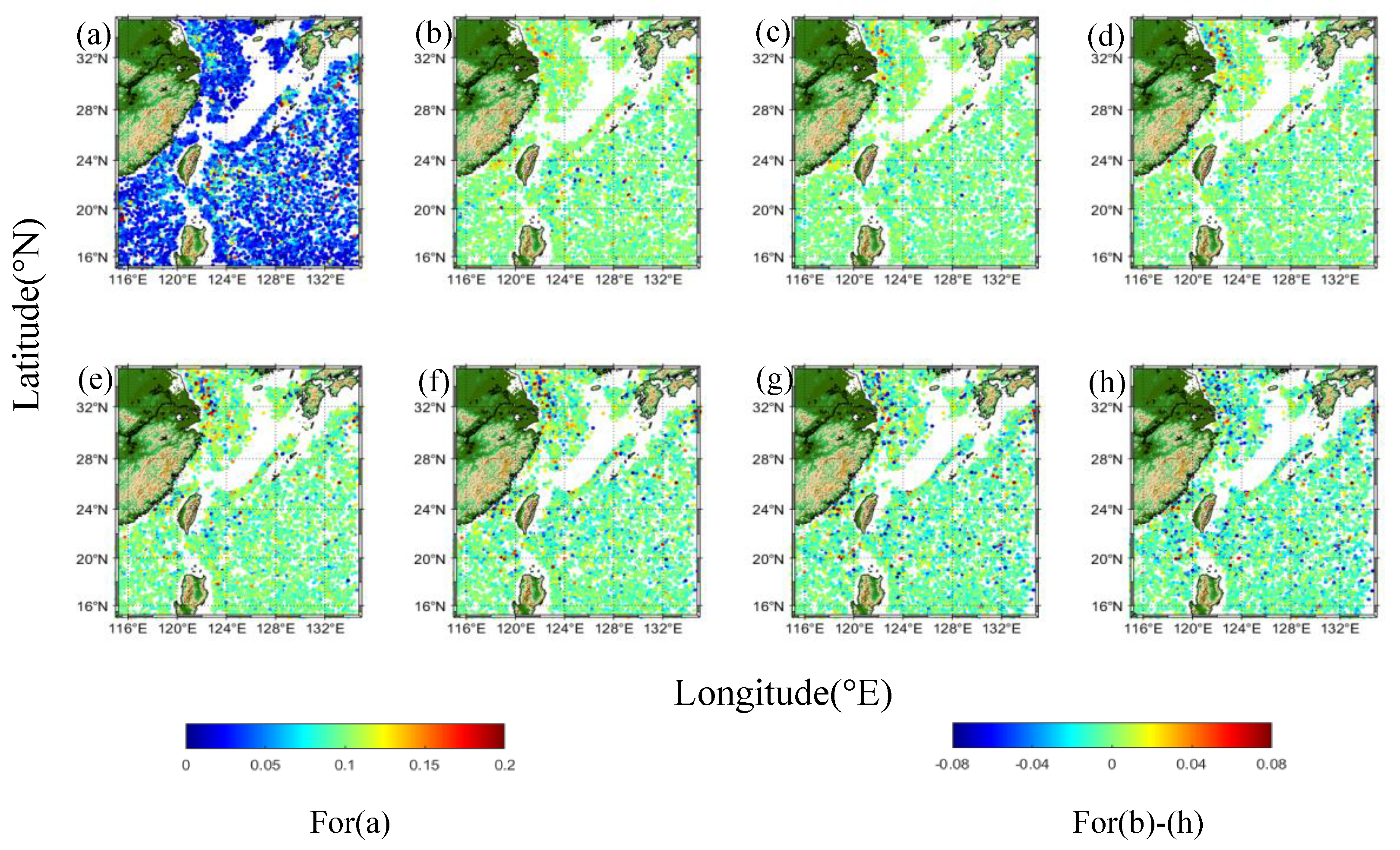
Figure 5.
(a) Scatterplot of the spatial distribution of the eddy radius (km) in the test set. And Figure 5 (b-h) Forecast errors (km) of eddy radii from day 1 to day 7.
Figure 5.
(a) Scatterplot of the spatial distribution of the eddy radius (km) in the test set. And Figure 5 (b-h) Forecast errors (km) of eddy radii from day 1 to day 7.
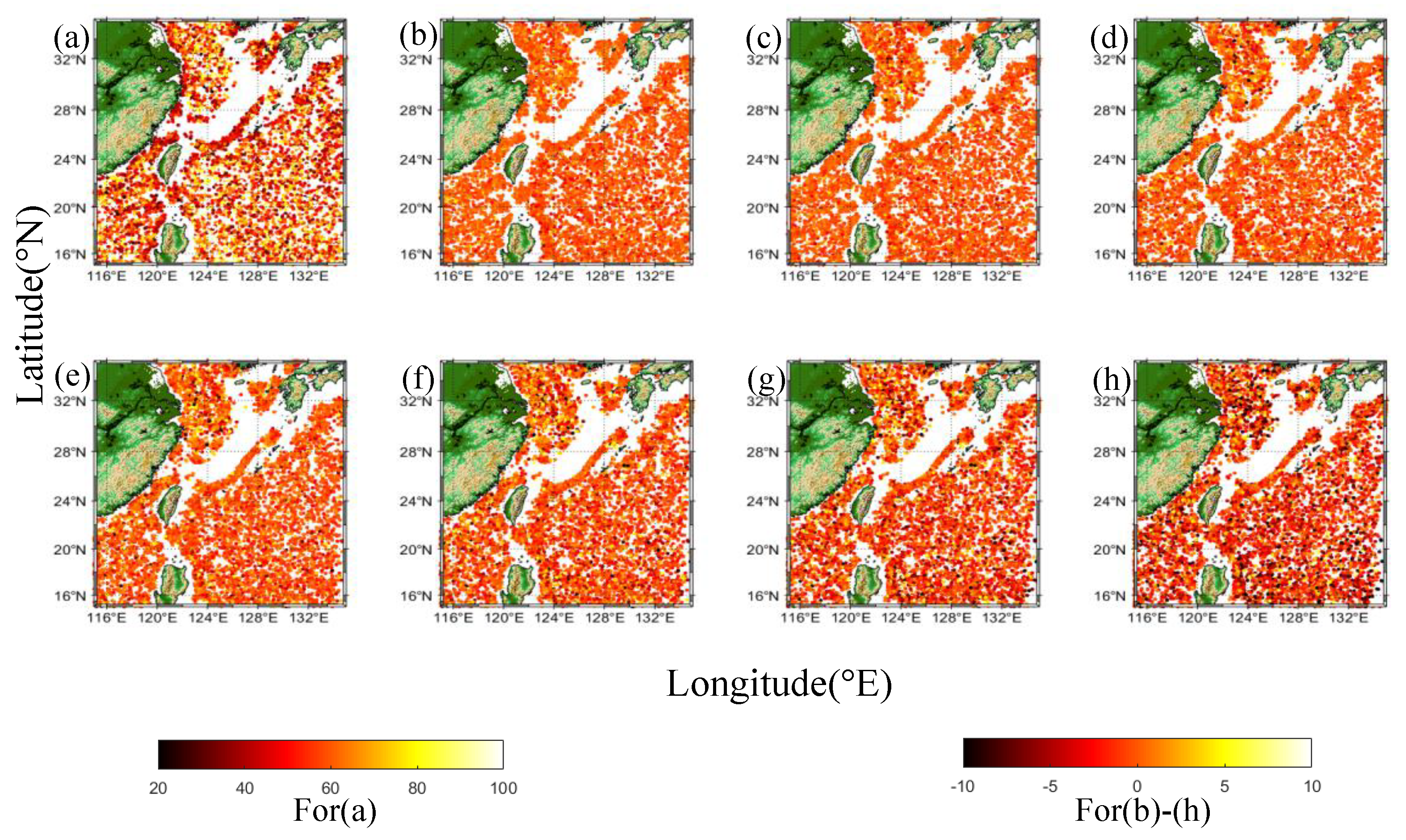
Figure 6.
(a) Scatterplot of the spatial distribution of eddy MCA (cm/s) in the test set. And Figure 6 (b-h) Forecast errors (cm/s) of eddy MCAs from day 1 to day 7.
Figure 6.
(a) Scatterplot of the spatial distribution of eddy MCA (cm/s) in the test set. And Figure 6 (b-h) Forecast errors (cm/s) of eddy MCAs from day 1 to day 7.
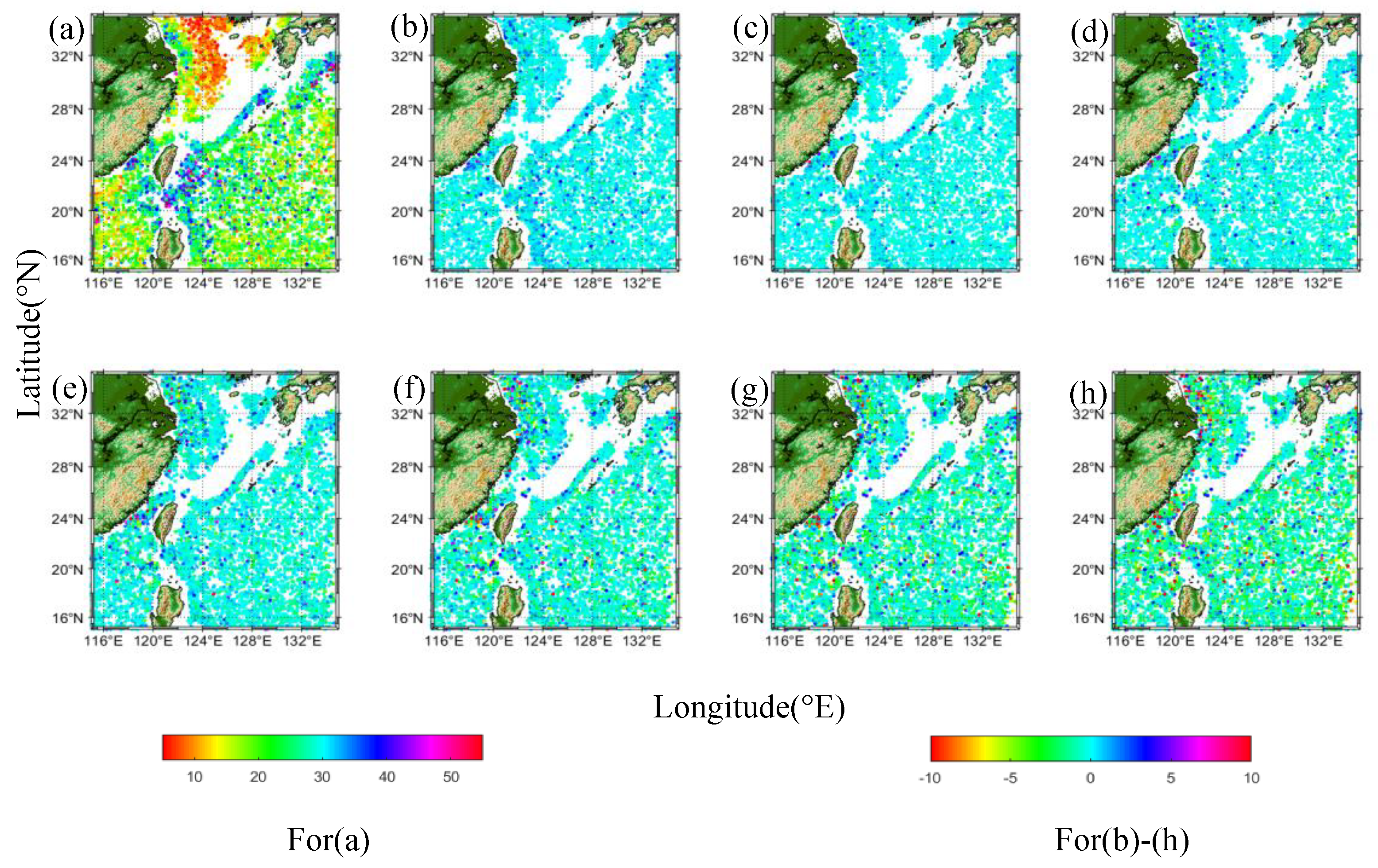
Figure 7.
Comparison of MAE between the proposed model and Wang et al. (2020) for amplitude, radius, and MCAs predictions.
Figure 7.
Comparison of MAE between the proposed model and Wang et al. (2020) for amplitude, radius, and MCAs predictions.
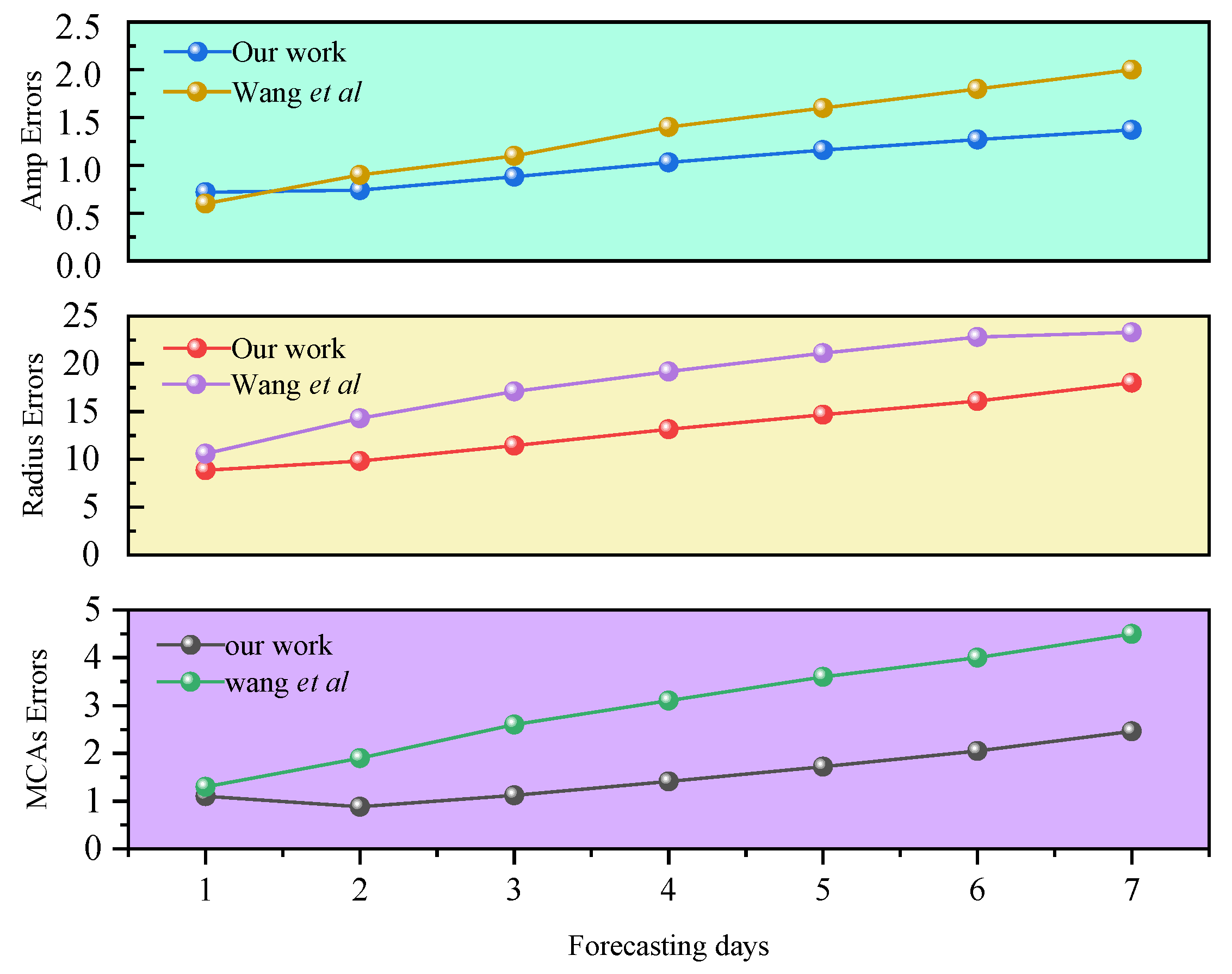
Figure 8.
Box-line plots of prediction results for three features with different physical information inputs, where type A is the initial condition, type B is the addition of EKE, type C is the addition of sea surface temperature, and type D is the addition of sea surface height.
Figure 8.
Box-line plots of prediction results for three features with different physical information inputs, where type A is the initial condition, type B is the addition of EKE, type C is the addition of sea surface temperature, and type D is the addition of sea surface height.
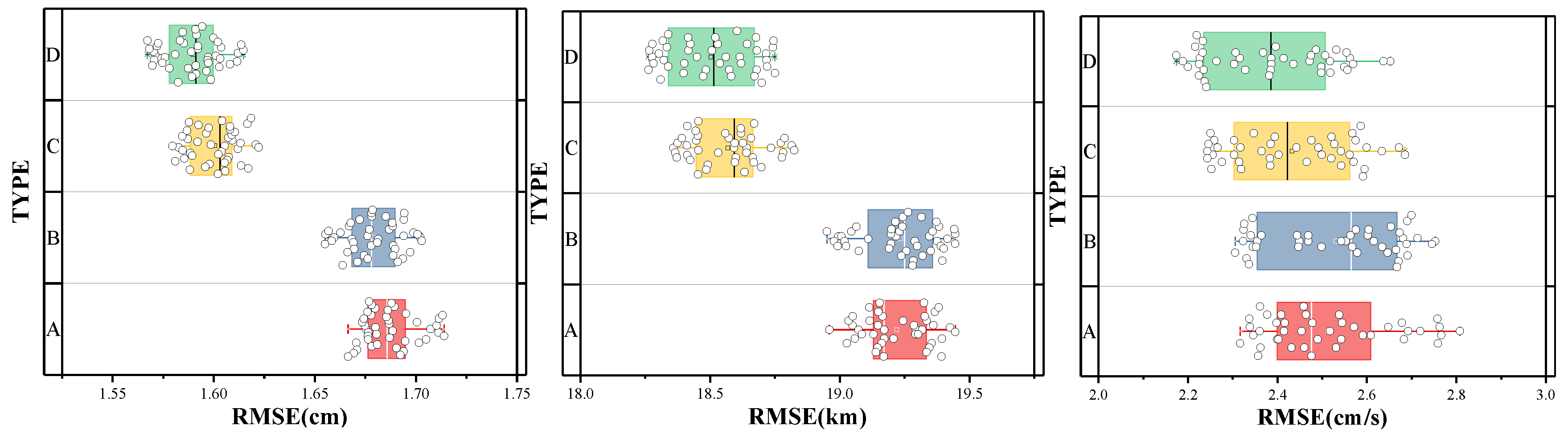
Figure 9.
RMSE. mean for amplitude, radius and MCA speed predictions for different years.
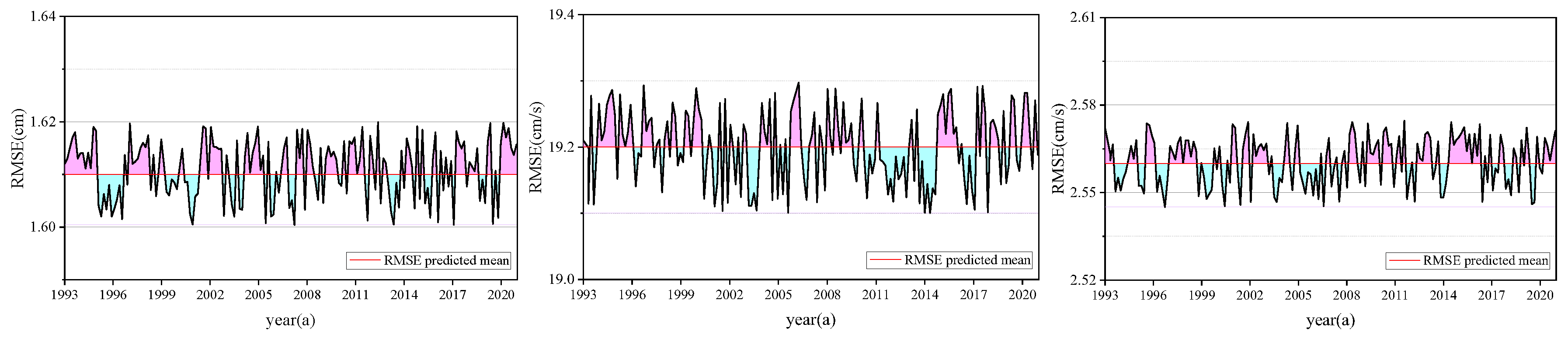

Table 1.
Prediction errors of eddy current characteristics in our work.
| Forecasting Days | 1st | 2nd | 3rd | 4th | 5th | 6th | 7th |
|---|---|---|---|---|---|---|---|
| Amplitude(cm) | 0.72 | 0.75 | 0.88 | 1.03 | 1.16 | 1.27 | 1.37 |
| Radius(km) | 8.85 | 9.82 | 1.14 | 1.32 | 1.47 | 1.61 | 1.80 |
| MCA Speed(cm/s) | 0.80 | 0.89 | 1.13 | 1.42 | 1.73 | 2.05 | 2.46 |
Table 2.
Prediction errors of eddy characteristics in different seasons.
| Summer | Winter | |
|---|---|---|
| Amp(cm) | 1.29 | 1.03 |
| Radius(km) | 15.3 | 13.2 |
| MCAs(cm/s) | 1.52 | 1.54 |
Disclaimer/Publisher’s Note: The statements, opinions and data contained in all publications are solely those of the individual author(s) and contributor(s) and not of MDPI and/or the editor(s). MDPI and/or the editor(s) disclaim responsibility for any injury to people or property resulting from any ideas, methods, instructions or products referred to in the content. |
© 2025 by the authors. Licensee MDPI, Basel, Switzerland. This article is an open access article distributed under the terms and conditions of the Creative Commons Attribution (CC BY) license (http://creativecommons.org/licenses/by/4.0/).
Copyright: This open access article is published under a Creative Commons CC BY 4.0 license, which permit the free download, distribution, and reuse, provided that the author and preprint are cited in any reuse.


