
Submitted:
23 October 2025
Posted:
24 October 2025
You are already at the latest version
Abstract
Long-term time series forecasting (LTSF) remains challenging, as models must capture long-range dependencies and remain robust to noise accumulation. Traditional recurrent architectures, such as Recurrent Neural Networks (RNNs) and Long Short-Term Memory (LSTM), often suffer from instability and information degradation over extended horizons. To address these issues, we propose the Kalman-Optimal Selective Long-Term Memory (KOSLM) model, which embeds a Kalman-optimal selective mechanism driven by the innovation signal within a structured state-space reformulation of LSTM. KOSLM dynamically regulates information propagation and forgetting to minimize state estimation uncertainty, providing both theoretical interpretability and practical efficiency. Extensive experiments across energy, finance, traffic, healthcare, and meteorology datasets show that KOSLM reduces mean squared error (MSE) by 10–30% compared with state-of-the-art methods, with larger gains at longer horizons. The model is lightweight, scalable, and achieves up to 2.5× speedup over Mamba-2. Beyond benchmarks, KOSLM is further validated on real-world Secondary Surveillance Radar (SSR) tracking under noisy and irregular sampling, demonstrating robust and generalizable long-term forecasting performance.
Keywords:
long-term time series forecasting
; LSTM
; state-space model
; Kalman Optimality
; selective memory
; robust prediction
; SSR tracking
1. Introduction
Long-term time series forecasting (LTSF) aims to predict future values over extended horizons based on historical observations. Accurate long-range forecasts are critical for applications such as energy scheduling, climate modeling, financial planning, traffic management, and healthcare resource allocation. LTSF presents unique challenges: capturing long-range dependencies, mitigating error accumulation, and adapting to non-stationary temporal dynamics [1].
Traditional recurrent architectures, including Recurrent Neural Networks (RNNs) [2] and Long Short-Term Memory (LSTM) networks [3,4], often struggle with long sequences due to vanishing or exploding gradients [5]. While LSTM gates alleviate some of these issues, their heuristic design lacks explicit structural constraints derived from a principled optimality criterion, potentially leading to suboptimal memory retention over extended horizons.
The Kalman filter (KF) [6] provides optimal state estimation under Gaussian noise [7]. Recent studies have explored integrating KF with LSTM to improve the accuracy of time-series forecasting. Representative approaches include: (i) Deep Kalman Filters [8], which parameterize the state-transition and observation functions of KF using LSTM; (ii) KalmanNet [9], which employs an LSTM to learn residual corrections to the Kalman gain under a known KF model; and (iii) uncertainty-aware LSTM–KF hybrids [10], which estimate the covariance or uncertainty structures of KF through recurrent dynamics. However, these approaches generally maintain a loose coupling between LSTM and KF — they do not embed Kalman-inspired feedback directly into the internal gating dynamics of LSTM.
Recently, selective state space models (S6) [11,12] have demonstrated efficient sequence modeling with linear-time complexity. By dynamically modulating SSM’s parameters based on the input, they can filter task-irrelevant patterns while retaining critical long-term information. This selective modulation property motivates revisiting LSTM gates from a state-space perspective, into which Kalman-inspired feedback can be injected, thereby endowing the gating mechanism with Kalman-optimal structural constraints.
In this work, we propose the Kalman-Optimal Selective Long-Term Memory (KOSLM) model, which establishes a context-aware feedback pathway that optimally balances memory retention and information updating, providing both theoretical interpretability and practical efficiency.
Our main contributions are as follows:
- State-space reformulation of LSTM: We formalize LSTM networks as input- and state-dependent state space models (SSMs), where each gate dynamically parameterizes the state-transition and input matrices. This framework provides a principled explanation of LSTM’s long-term memory behavior.
- Kalman-optimal selective gating: Inspired by the Kalman filter and selective SSMs, we introduce a Kalman-optimal selective mechanism in which the state-transition and input matrices are linearly modulated by a Kalman gain learned from the innovation term, establishing a feedback pathway that minimizes state estimation uncertainty.
- Applications to real-world forecasting: KOSLM consistently outperforms state-of-the-art baselines across long-term time series forecasting (LTSF) benchmarks in energy, finance, traffic, healthcare, and meteorology, achieving 10–30% lower mean squared error (MSE) and up to 2.5× faster inference compared with Mamba-2. In real-world Secondary Surveillance Radar (SSR) tracking under noisy and irregular sampling, KOSLM demonstrates strong robustness and generalization ability.
By bridging heuristic LSTM gating with principled Kalman-optimal estimation, KOSLM provides a robust, interpretable, and scalable framework for long-term sequence modeling, offering both methodological novelty and practical forecasting utility.
2. Background and Theory
2.1. LSTM Networks
RNNs model sequential data through recursive temporal computation. However, traditional RNNs often suffer from vanishing and exploding gradients when capturing long-term dependencies. The LSTM network [3] addresses this issue by introducing gating mechanisms that regulate the flow of information over time. The network structure of the LSTM neuron is shown in Figure 1.
Each LSTM unit maintains a cell state that carries long-term information and a hidden state that provides short-term representations. The cell state is updated according to:
where , , and denote the forget, input, and output gates, respectively. These gates are nonlinear functions of the current input and the previous hidden state . The final output is obtained as:
This gating mechanism allows the model to selectively retain or discard information, mitigating gradient degradation. However, the gates are learned heuristically through data-driven optimization rather than derived from an explicit structural optimality constraint, making the LSTM sensitive to noise and unstable for long-term dependencies.
2.2. State Space Models
2.2.1. Selective State Space Models
S6 are a recent class of sequence models for deep learning that are broadly related to RNNs and classical SSMs. They are inspired by a particular system (Equation (3)) that maps a 1-dimensional function or sequence through an implicit latent state :
These models integrate the SSM described above into deep learning frameworks and introduce input-dependent selective mechanisms (see Appendix A for a detailed discussion), achieving Transformer-level modeling capability with linear computational complexity.
The theoretical connections among LSTM, KF, and SSM provide the foundation for constructing a unified Kalman-optimal selective memory framework.
2.2.2. Kalman Filter
The KF [6] is a classical instance of the state-space model, providing the minimum mean-square-error (MMSE) estimate of hidden system states under noisy observations. The system dynamics are expressed as:
where A and M are the state transition and observation matrices; and denote process and observation noise with covariances and , respectively. Note that the observation can be regarded as the input in the SSMs.
At each time step, the KF performs two operations: prediction and update. The prediction step estimates the prior state:
while the update step refines this prediction using the observation :
Here, is the Kalman gain, which minimizes the posterior estimation error covariance. It determines how much new information (the innovation term ) should be incorporated into the updated state. This principle of optimal selective information integration forms the theoretical foundation for the innovation-driven gating design proposed later. A detailed justification for interpreting the Kalman gain as a prototype of dynamic selectivity is provided in Appendix B.1
3. Proposed Method
3.1. Reformulating LSTM as a State-Space Model
Following the LSTM formulation in Equation (1), the LSTM cell can be equivalently reformulated as a time-varying SSM, where the cell state evolves under nonlinear, input- and state-dependent dynamics:
Here, serves as the observation in the KF (corresponding to the input in the SSM and LSTM), and the matrices and are determined by the forget gate and input gate , respectively. A detailed derivation of this LSTM-to-SSM reconstruction, including the mapping of gating mechanisms to state-space parameters, is provided in Appendix B.2.
3.2. Kalman-Optimal Selectivity via Innovation-Driven Gain
We introduce the innovation term from the KF:
which measures the discrepancy between the observation input and the predicted state based on the previous cell state , serving as a real-time correction signal between model prediction and actual measurement.
In classical KF, this innovation drives the computation of the Kalman gain (Equation (6)), which regulates the incorporation of new information and the retention of prior state during the update step. In KOSLM, rather than explicitly solving the Riccati recursion [13], we learn a functional mapping:
where is a lightweight neural module implemented as a two-layer MLP with sigmoid activation, parameterized by . The use of the sigmoid ensures that the estimated gain , maintaining physical interpretability as an adaptive weighting coefficient and preventing numerical instability.
The learned gain dynamically regulates the trade-off between prior memory and new information, yielding a learnable yet principled mechanism for Kalman-optimal selectivity. The bounded output range of further stabilizes the state-space update and constrains divergence during long-horizon inference. Appendix B.3 provides the theoretical derivation demonstrating that the innovation term serves as a sufficient statistic for learning the Kalman gain. Appendix B.4 further presents controlled experiments confirming that the learned gain accurately approximates the oracle Kalman gain across various regimes (Table A1). These results jointly establish the theoretical and empirical foundation for embedding Kalman-optimal selectivity into deep learning models.
We then define the state-space evolution as:
where A is the base state transition matrix, serving as a learnable parameter of the model.
The KOSLM network architecture is illustrated in Figure 2, mirroring the classical Kalman update while maintaining differentiability and learnability.
3.3. Structural Overview of KOSLM
The KOSLM cell preserves the computational efficiency of a standard LSTM while embedding a Kalman-inspired feedback loop. At each timestep, the operations are:
- Compute the innovation: ;
- Estimate the Kalman gain: ;
- Update state transition matrices: , ;
- Propagate the hidden state: ;
- Compute the output hidden representation: .
3.4. Theoretical Interpretation
Under linear–Gaussian assumptions and with a sufficiently expressive mapping , the learned gain converges to the oracle Kalman solution. Consequently, KOSLM inherits the nonlinear expressive power of LSTM while achieving the minimum-variance estimation property of the Kalman filter in its linear regime. This leads to improved stability and robustness, particularly in long-horizon or noisy sequence modeling.
3.5. Practical Advantages
KOSLM offers several practical benefits:
- Robustness: The feedback structure mitigates error accumulation and improves performance under noise or distributional shifts.
- Efficiency: With only 0.24M parameters, KOSLM achieves up to 2.5× faster inference than Mamba-2, while maintaining competitive accuracy.
- Versatility: The model generalizes across diverse domains, from energy demand forecasting to radar-based trajectory tracking.
4. Results
This section provides a comprehensive evaluation of the proposed KOSLM model through large-scale long-term forecasting benchmarks (§Section 4.1), component ablation studies (§Section 4.2), efficiency assessments (§Section 4.3), and a real-world radar trajectory tracking case study (§Section 4.4). The experimental analyses collectively aim to validate both the predictive accuracy and robustness of KOSLM across diverse and noisy temporal conditions.
4.1. Main Experiments on Benchmark Datasets
To examine the capability of KOSLM in modeling long-range dependencies and maintaining stability over extended forecasting horizons, we conduct systematic experiments on nine widely used real-world datasets covering domains such as traffic flow, electrical load, exchange rate, meteorology, and epidemiology. The datasets vary in frequency, dimensionality, and temporal regularity, providing a comprehensive benchmark for assessing model generalization.
4.1.1. Dataset Details
We summarize the datasets used in this study as follows. Weather [16] contains 21 meteorological variables (e.g., temperature and humidity) recorded every 10 minutes throughout 2020. ETT (Electricity Transformer Temperature) [17] includes four subsets: two hourly-level datasets (ETTh1, ETTh2) and two 15-minute-level datasets (ETTm1, ETTm2). Electricity [18], derived from the UCI Machine Learning Repository, records hourly power consumption (kWh) of 321 clients from 2012 to 2014. Exchange [19] comprises daily exchange rates among eight countries. Traffic [20] consists of hourly road occupancy rates measured by 862 sensors on San Francisco Bay Area freeways from January 2015 to December 2016. Illness (ILI) dataset [21] tracks the weekly number of influenza-like illness patients in the United States. Table 2 summarizes the statistical properties of all nine benchmark datasets. All datasets are divided into training, validation, and test subsets with a ratio of 7:1:2.
4.1.2. Implementation Details
All models are trained using the Adam optimizer without weight decay. The learning rate is selected from via grid search. Batch size is set to 32 by default, adjustable up to 256 depending on GPU memory. Training is performed for 15 epochs, and the checkpoint with the lowest validation loss is used for testing. Experiments are repeated five times, and average results are reported. All models adopt a 2-layer architecture with hidden dimension 64. We use PyTorch’s default weight initialization, and no additional regularization (dropout or gradient clipping) is applied. All experiments are implemented in PyTorch 2.1.0 with Python 3.11 on NVIDIA RTX 4090 GPUs. Random seeds for Python, NumPy, and PyTorch are fixed to ensure reproducibility.
The gain function is implemented as a one-layer MLP with hidden dimension 64 and sigmoid activation, followed by a linear projection to the gain matrix . The same network is shared across all timesteps to ensure parameter consistency.
4.1.3. Experimental Setup
All experiments follow the evaluation protocol established in xLSTMTime [22], adopting prediction horizons of for standard datasets and for the weekly-sampled ILI dataset. We compare the proposed KOSLM with nine recent state-of-the-art baselines that represent diverse architectural paradigms, spanning state-space, recurrent, attention-based, and linear modeling frameworks:
- LSTM-based: xLSTMTime [22];
This comprehensive selection enables a fair and systematic comparison across diverse sequence modeling paradigms.
4.1.4. Overall Performance
Table 3 and Table 4 report the long-term multivariate forecasting results on nine real-world datasets, evaluated by mean squared error (MSE) and mean absolute error (MAE). Across nearly all datasets and prediction horizons, the proposed KOSLM achieves the best or near-best performance, highlighting its superior generalization and robustness under diverse temporal dynamics.
- Consistent superiority across domains: KOSLM outperforms all competing baselines, particularly under complex and noisy datasets such as Traffic, Electricity, and ILI. In terms of average MSE reduction, KOSLM achieves relative improvements of +31.96% on Traffic, +13.37% on Electricity, +5.47% on Exchange, +11.26% on Weather, and +22.04% on ILI. Moreover, on the four ETT benchmarks (ETTh1/2, ETTm1/2), KOSLM yields steady improvements ranging from 4.03% to 27.46%, demonstrating strong adaptability to varying periodic and nonstationary patterns. These consistent gains verify that the Kalman-inspired selective updating mechanism effectively filters noise and dynamically adjusts to regime shifts, leading to stable forecasting accuracy over long horizons.
- Stable error distribution and reduced variance: The MSE–MAE gap of KOSLM remains narrower than that of other baselines, implying reduced large deviations and more concentrated prediction errors. This indicates more stable error behavior, which is crucial for long-horizon forecasting where cumulative drift often occurs. The innovation-driven Kalman gain estimation provides adaptive correction at each timestep, ensuring smooth and consistent prediction trajectories under uncertain dynamics.
- Strong scalability and generalization: KOSLM achieves leading performance not only on large-scale datasets (Traffic, Electricity) but also on small, noisy datasets (ILI), confirming robust generalization across different temporal resolutions and noise levels. Its consistent advantage over Transformer-based (e.g., iTransformer, FEDFormer, PatchTST), recurrent (e.g., xLSTMTime), and state-space models (e.g., S-Mamba, FiLM) demonstrates that the proposed Kalman-optimal selective mechanism provides an effective inductive bias for modeling long-term dependencies.
- Advantage over LSTM-based architectures: Compared with advanced LSTM-based models such as xLSTMTime, KOSLM achieves consistently better results across nearly all datasets and horizons. This verifies that replacing heuristic gates with Kalman-optimal selective gating enhances memory retention and update stability. While xLSTMTime alleviates gradient decay via hierarchical memory, KOSLM further refines state updates through innovation-driven gain estimation, thereby achieving a more principled and stable information flow.
To further demonstrate the long-horizon stability of the proposed model, we compare KOSLM with the recent S-Mamba [24], a state-of-the-art state space model that represents the latest advancement in efficient sequence modeling. Figure 3 presents the forecasting trajectories at the long horizon () across five representative datasets. KOSLM maintains accurate trend alignment and amplitude consistency with the ground truth, showing particularly superior convergence behavior on smoother and more stationary datasets such as Weather and Exchange, where the Kalman gain adaptation stabilizes long-term predictions. In contrast, S-Mamba exhibits slight temporal lag and amplitude attenuation under extended forecasting conditions. These results visually confirm the advantage of the proposed Kalman-based feedback selectivity in preserving long-term temporal fidelity.
4.2. Ablation Study
To further analyze the effectiveness of each proposed component, we conduct ablation experiments on four widely used long-term time-series forecasting datasets (ETTm1, ETTh1, Traffic, and Exchange) with a prediction length of , following the data preprocessing described in Section 4.1.1. All model variants are trained and tested following the default implementation settings described in Section 4.1.2, and the results are averaged over five runs to ensure statistical reliability.
4.2.1. Structural Ablation.
We first evaluate the contribution of the Kalman-based structure by comparing three variants: (i) Full (KOSLM): the complete model where and ; (ii) No-Gain: receives the innovation but directly outputs , removing the explicit Kalman gain variable; (iii) No-Innov: receives the standard network input (e.g., ) instead of the innovation, while is still mapped to via the Kalman form.
As shown in Table 5, removing either the gain computation or the innovation input consistently leads to higher errors across all datasets. For instance, on ETTm1, the MSE increases by 32.9% when the gain path is removed, confirming that both the innovation statistic and Kalman gain are essential for stable long-horizon prediction. This finding aligns with the Kalman filtering principle that the innovation serves as a sufficient statistic for state correction.
4.2.2. Capacity Ablation
To verify that the performance gains of KOSLM mainly stem from the Kalman-optimal structural design rather than the network capacity, we conduct a capacity ablation study. We evaluate the network under four progressively larger configurations: (i) Linear: a single linear layer with input dimension equal to the number of input features and output dimension 64, without any activation; (ii) SmallMLP: a two-layer MLP with 128 hidden units and sigmoid activation; (iii) MediumMLP: a three-layer MLP with 256 hidden units per layer and Rsigmoid activation; (iv) HighCap: a four-layer MLP with 512 hidden units per layer and sigmoid activation.
All models are trained under identical settings with five independent random seeds, and the results are reported as mean ± standard deviation. This allows us to evaluate both performance trends and statistical reliability. From Table 6, it is evident that increasing the network capacity beyond SmallMLP does not consistently improve MSE or MAE; in some cases, the error even increases slightly. The small MediumMLP improvements (ETTm1) or slight deterioration (ETTh1, Traffic, Exchange) indicate that performance gains are dominated by the Kalman-optimal structural design rather than network depth or over-parameterization. This confirms the effectiveness of the innovation-driven gain estimation in KOSLM for stable long-horizon prediction.
4.3. Efficiency Benchmark
To evaluate the computational efficiency of KOSLM, we benchmark it against representative sequence modeling baselines, including Transformer, Mamba-2, and LSTM, across four key metrics: runtime scalability, end-to-end throughput, memory footprint, and parameter count. All experiments are conducted using PyTorch 2.1.0 with torch.compile optimization on a single NVIDIA RTX 4090 GPU.
4.3.1. Runtime Scalability
We assess runtime performance on both a controlled synthetic setup and the ETTm1 dataset. As illustrated in Figure 4, KOSLM exhibits near-linear growth in inference time with increasing sequence length L. For sequences longer than , KOSLM surpasses optimized Transformer implementations (FlashAttention [31]) and achieves up to faster execution than the fused-kernel version of Mamba-2 [24] at . Compared with a standard PyTorch LSTM, KOSLM achieves approximately – speedup across the tested sequence lengths, demonstrating robust scalability for long sequences.
4.3.2. Throughput Analysis.
Figure 5 reports the end-to-end inference throughput measured in million tokens/s (M tokens/s). KOSLM maintains consistently high throughput across all tested sequence lengths, achieving up to higher throughput than LSTM and higher than Mamba-2 in the 4K–8K regime. The performance remains stable for even longer sequences, highlighting the model’s suitability for extended temporal dependencies.
4.3.3. Memory Footprint.
Table 7 reports GPU memory usage during training for varying batch sizes with input length 2048 and models containing approximately 0.24M parameters. KOSLM demonstrates favorable memory efficiency relative to similarly sized Mamba-2 implementations and remains comparable to a standard LSTM with roughly ten times more parameters. This efficiency results from KOSLM’s compact Kalman-optimal selective mechanism, which dynamically modulates state transitions with minimal parameter overhead.
4.3.4. Model Size.
Table 8 summarizes the parameter counts. KOSLM contains only 0.24M parameters, roughly 4.5% of the Transformer and 11% of the LSTM baselines, while achieving comparable or superior forecasting performance. The compact design emphasizes KOSLM’s suitability for deployment in resource-constrained environments.
This efficiency stems directly from the Kalman-optimal selective mechanism, which adaptively regulates the state update through innovation-driven gain modulation. Such a formulation not only reduces redundant computation but also provides a principled pathway for scaling to long sequences.
4.4. Real-world Application: SSR Target Trajectory Tracking
To further evaluate the robustness and practical generalizability of KOSLM under real-world noisy conditions, we conducted a real-world experiment on secondary surveillance radar (SSR) target trajectory tracking. SSR is a ground-based air traffic surveillance system where aircraft respond to radar interrogations with encoded transponder signals, generating sparse range–azimuth sequences known as raw SSR plots. These observation sequences present three major challenges for sequential modeling:
- High stochastic noise: Measurement noise leads to random fluctuations in the estimated positions;
- Irregular sampling: Aircraft maneuvers and radar scan intervals result in uneven temporal spacing;
- Correlated anomalies: Spurious echoes or missing detections introduce discontinuities in the trajectories.
These characteristics make SSR a natural yet challenging testbed for assessing model stability, noise resilience, and temporal consistency. KOSLM addresses these challenges by integrating context-aware selective state updates with learnable dynamics under the Kalman optimality principle, enabling robust filtering, smoothing, and extrapolation in partially observed environments.
4.4.1. Experimental Setup
To achieve a balance between realism and experimental controllability, we adopted a semi-physical simulation approach. Training data were derived from Automatic Dependent Surveillance–Broadcast (ADS-B) flight tracks obtained from the OpenSky Network [32]. Controlled Gaussian noise with an SNR of 33 dB was added to emulate SSR observation uncertainty. For evaluation, we deployed KOSLM on real SSR radar data collected from an operational ground-based system (peak transmit power 6 kW), capturing eight live air-traffic targets under operational conditions. Detailed data acquisition and preprocessing procedures are provided in Appendix C.
Unlike the main benchmarking experiments on standardized long-term time series forecasting (LTSF) datasets, this case study aims to demonstrate practical applicability and operational robustness. Due to irregular sampling, sparse observations, and high stochastic noise, conventional quantitative metrics such as MSE or MAE are not meaningful. Therefore, we focus on qualitative trajectory visualizations to illustrate model performance in realistic conditions.
4.4.2. Results and Analysis
Figure 6 presents representative trajectories of eight air-traffic targets, comparing classical KF algorithm, Transformer, Mamba, and KOSLM. The classical KF algorithm exhibits locally inaccurate and jagged trajectories due to its fixed linear dynamics, which cannot adapt to irregular sampling or abrupt maneuvers. The Transformer captures general trends but produces fragmented and temporally inconsistent tracks under sparse and noisy observations. Mamba improves noise robustness but still demonstrates local instability during complex maneuvers.
In contrast, KOSLM generates smooth, coherent, and temporally consistent trajectories that closely follow the true flight paths, highlighting its ability to handle high stochastic noise, irregular sampling, and correlated anomalies. This robustness stems from the innovation-driven Kalman gain and context-aware selective state updates, which allow KOSLM to adapt dynamically to non-stationary motion patterns.
5. Conclusions
This study addressed a fundamental limitation of recurrent architectures such as LSTM, whose heuristically designed gates lack structural constraints for optimality, leading to instability and information decay over long sequences. To overcome this issue, we proposed the Kalman-Optimal Selective Long-Term Memory Network (KOSLM), which reconstrues LSTM as a nonlinear, input- and state-dependent state-space model, and integrates an innovation-driven Kalman-optimal gain path for principled information selection. This formulation unifies LSTM gating, selective state-space modeling, and Kalman filtering into a single theoretically grounded recurrent framework.
Extensive experiments demonstrate that KOSLM achieves state-of-the-art performance on long-term forecasting benchmarks, while ablation studies confirm the essential role of the innovation statistic and Kalman-form gain in stabilizing long-horizon modeling. Moreover, validation on real-world SSR trajectory tracking highlights its robustness under noisy and non-stationary conditions. In summary, embedding Kalman-optimal principles into deep recurrent networks provides both theoretical insights and practical benefits for robust long-term sequence modeling. Future work will focus on extending KOSLM beyond Gaussian assumptions and applying it to multimodal and cross-domain time-series scenarios.
Author Contributions
All authors contributed to the conception and design of the study. Material preparation, code implementation, data collection, and analysis were performed by Xin Tan and Lei Wang. The first draft of the manuscript was written by Lei Wang, and all authors commented on previous versions of the manuscript. Xin Tan and Mingwei Wang supervised the research and provided critical revisions and theoretical guidance. Ying Zhang assisted in data verification and manuscript editing. All authors read and approved the final manuscript.
Funding
This research received no external funding.
Data Availability Statement
The datasets and source code used in this study are publicly available at https://github.com/wl822513/KOSLM.
Conflicts of Interest
The authors declare no conflicts of interest.
Appendix A. Selective State Space Models
This section focuses on S6, which provide a unified framework connecting the gating with time-varying state-space representations. Their associated selection mechanisms have become a central design principle in modern SSMs, such as Mamba [11]. These mechanisms improve modeling efficiency by dynamically identifying and retaining task-relevant information over long sequences, effectively compressing the latent state without compromising representational capacity.
- Relation to Existing Concepts
Selection mechanisms are conceptually related to several prior ideas, including gating, hypernetworks, and data-dependent parameterization:
- Gating was originally introduced as a signal-control mechanism in recurrent neural networks (RNNs) such as LSTM [3] and GRU [33], where multiplicative gates regulate information updates across time steps. The concept has been generalized to other architectures, including gated convolutions and transformers [34,35], though often without an explicit interpretation in terms of temporal signal control.
- Hypernetworks [36] generate network parameters dynamically through auxiliary networks, enabling the model’s internal dynamics to adapt based on input signals.
- Data-dependent parameterization [37] represents a broader paradigm in which model parameters are directly conditioned on input data. Both gating and hypernetworks can be viewed as specific instances within this larger class.
While selection mechanisms share certain similarities with these paradigms, they form a distinct modeling category. Unlike classical gating or hypernetwork mechanisms that often operate locally or step-wise, selection mechanisms are explicitly designed to route, filter, or suppress sequence-level information in an input- or state-dependent manner, enabling stable long-horizon modeling. In selective SSMs, this is typically realized by parameterizing system matrices (e.g., , A, B, C) as functions of the input at each time step.
- From Implicit to Explicit Selection
Early structured SSMs (S4) [38] encoded fixed inductive biases through learned structured dynamics, providing an implicit, input-independent form of selection via controlled signal propagation. Later models, including Mamba [11], introduced explicit selection, where the parameters of the state-space system (e.g., , A, B, C) are conditioned directly on the current input, allowing the model to dynamically emphasize or suppress features at each step.
- Semantic Clarification
As discussed in S6 [11], while selection mechanisms can be loosely related to gating, hypernetworks, or general data dependence, these broader descriptions do not capture the defining characteristic of selection. The term selection is reserved for mechanisms that explicitly operate along the sequence dimension, enabling adaptive memory compression and long-range information control. From a dynamical systems perspective, such mechanisms can be interpreted through state-space discretization and signal propagation theory [39,40]. Importantly, classical RNN gating can be viewed as a local, step-wise precursor to these more general selection mechanisms.
- Scope and Relevance
The principle of selection underlies recent progress in linear-time sequence modeling. Building upon this paradigm, our proposed KOSLM extends selective SSMs by introducing an innovation-driven Kalman-optimal feedback pathway, transforming heuristic selection into a principled, uncertainty-aware mechanism for long-term sequence modeling.
Appendix B. Detailed Derivation
Appendix B.1. Kalman Gain as a Prototype for Dynamic Selectivity
In classical filtering theory, the Kalman gain acts as a dynamic weighting factor that determines how prior state estimates and new observations are combined to produce a new state [6]. It is formally derived as the solution to the Riccati differential equation, and its value depends on the evolving uncertainty in the internal system state (captured by the prior covariance ) and the noise characteristics of the observation process (captured by the measurement covariance R) [41]. This time-varying gain governs the extent to which incoming measurements correct the state estimate, ensuring minimum mean-squared error under Gaussian noise assumptions.
This correction process is essentially a trade-off between the historical state information of the system and the incoming input information. In the context of deep learning, we interpret the observation as the current input sequence, and the prior state estimate as the latent representation of the system’s history. From this perspective, the Kalman gain plays a role analogous to a dynamic selection factor that balances the contribution of contextual knowledge (from the model state) and content information (from the input) in generating the updated representation. Therefore, the Kalman gain can be viewed as a principled prototype for content-aware and context-sensitive information selection. This perspective justifies the broader use of dynamic selection strategies in sequence models, especially when aiming to balance stability and adaptability in long-range modeling.
Appendix B.2. LSTM-to-SSM Reconstruction
To endow LSTM networks with structured modeling semantics, in this section we reconstruct them as a form of nonlinear time-varying state-space model ((see Equation (3a)). Specifically, we identify that the interactions among the forget gate, input gate, output gate, input signal, and cell state in LSTMs essentially constitute an input-dependent and state-aware state transition–observation process.
As illustrated in Figure 1, the gating mechanisms and the cell state in LSTM establish a pathway for memory propagation across time. The cell state is the core component that preserves long-term memory across the temporal dimension and models long-range dependencies. In terms of representational role, it is both semantically and structurally equivalent to the latent state in SSMs (see Equation (3a)). Therefore, we take as the central axis and analyze its information propagation process.
The forget gate regulates the degree to which short-term memory from cell state is discarded. It is determined jointly by the current input and the previous hidden state , thereby embodying an input- and state-dependent transition process:
where denotes the concatenated input. The corresponding retained term is .
The pathway for new information input in LSTM consists of two steps:
- The candidate cell state can be interpreted as a differentiable nonlinear mapping from the joint input :where the linear transformation fuses the external input and the hidden state into the observation space, with introducing nonlinearity to produce an intermediate representation . We treat this representation as the observation input at time t under the SSM.1
- The interaction between the input gate and the candidate state establishes a structured pathway for injecting new information into the state dynamics, analogous to the excitation of state evolution by external inputs in SSMs.where serves as the input matrix, structurally equivalent to the input gate .
Consequently, the update process of the LSTM cell state at time t (Eq.1) can be rewritten in the form of a state-space transition:
where and are realized through the forget and input gates driven by the joint input , thereby endowing the model with the ability to selectively forget or memorize long-term information in an input-dependent and context-aware manner.
Finally, the output pathway of LSTM is given by
which is formally equivalent to the observation equation of a classical SSM:
where is formed by the output gate together with the nonlinear transformation .
The above reconstruction shows that the gating mechanism in LSTM can be interpreted as a class of nonlinear, input- and state-dependent SSMs. This perspective establishes a valid unification of LSTM gating mechanisms and state-space models, and reveals that LSTM’s long-term memory capability originates from the structured realization of both state-space modeling and efficient information selection. Building on this understanding, we further introduce the Kalman gain into this state-space structure, imposing a structural constraint that minimizes the uncertainty of state estimation errors.
Appendix B.3. Kalman-Optimal Selective Mechanism
Recent studies on time series modeling have proposed a class of selective mechanisms based on SSMs, among which the most representative work is S6 [11]. Its core idea points out:
“One method of incorporating a selection mechanism into models is by letting their parameters that affect interactions along the sequence (e.g., the recurrent dynamics of an RNN or the convolution kernel of a CNN) be input-dependent.”
Inspired by this, we design a selective mechanism based on Kalman-optimal state estimation within the SSM (Equation (3)). Unlike the input-dependent selection mechanism represented by S6, we make the key parameters (, ), which control how the model selectively propagates or forgets information along the sequence dimension, depend on the innovation term: the deviation between the observation input and the prior state prediction in the observation space, denoted as in this paper. This method constructs a learnable selection path that integrates observational inputs and latent state feedback, with the optimization objective of minimizing the uncertainty in state estimation errors.
- Learnable Gain from Innovation
In the KF algorithm, the closed-form solution of the Kalman gain (Equation (6)) is obtained by minimizing the covariance of the state estimation error [6]. Here, the observation matrix and the observation noise covariance are considered known system priors, usually derived from physical modeling or domain knowledge. Therefore, the dynamics of entirely stem from the statistical properties of the prior estimation error . Under the linear observation model (4b), is mapped into the observation space, yielding the following representation of the innovation term:
This equation shows that is a linear mapping of , which, although perturbed by additive observation noise , still retains the full uncertainty information of . Thus, can serve as a sufficient statistic for estimating , providing a theoretical basis for directly estimating from the innovation term. The estimation process is defined as:
where is a differentiable nonlinear function, parameterized by a neural network and trained via gradient descent. Theoretical soundness of this formulation is confirmed by a controlled experiment (Appendix B.4), which demonstrates that can reliably recover the oracle Kalman gain from the innovation statistics with negligible estimation error.
- Optimal Selectivity via Gain
By substituting the KF prediction process (Equation (5)) into the state update equation (Equation (7)), the two processes can be expressed as a nonlinear time-varying SSM form (Equation (3a)):
Within this framework, parameters and are linearly modulated by driven by the innovation term, yielding a context-aware Kalman-optimal selective path that minimizes state estimation uncertainty and imposes structural optimality constraints on LSTM.
Appendix B.4. Empirical Validation of Innovation-Driven Kalman Gain Learning
To empirically validate the theoretical claim that the Kalman gain can be dynamically inferred from the innovation term, we design a controlled linear–Gaussian synthetic experiment where the optimal gain has a closed-form solution. This allows us to directly compare the learned gain against the ground-truth Kalman gain and quantify their alignment over time.
- Experimental Design
We consider a one-dimensional linear dynamical system as in Equation (4). The analytical Kalman gain is computed from the standard Riccati recursion and serves as the oracle reference. We design three model variants for comparison:
- (i)
- Oracle-KF: Standard Kalman filter using the known parameters to compute .
- (ii)
- Supervised-: A small MLP takes the innovation as input and predicts , trained by minimizing over all timesteps. During training, the predicted prior state is provided by the Oracle-KF to isolate the learning of the innovation-to-gain mapping. This tests whether the innovation term contains sufficient information to recover the oracle gain.
- (iii)
- End-to-End: The same MLP is trained to directly map from to without explicitly constructing the innovation term, serving as an ablation to assess the importance of innovation-driven modeling.
- Setup and Metrics
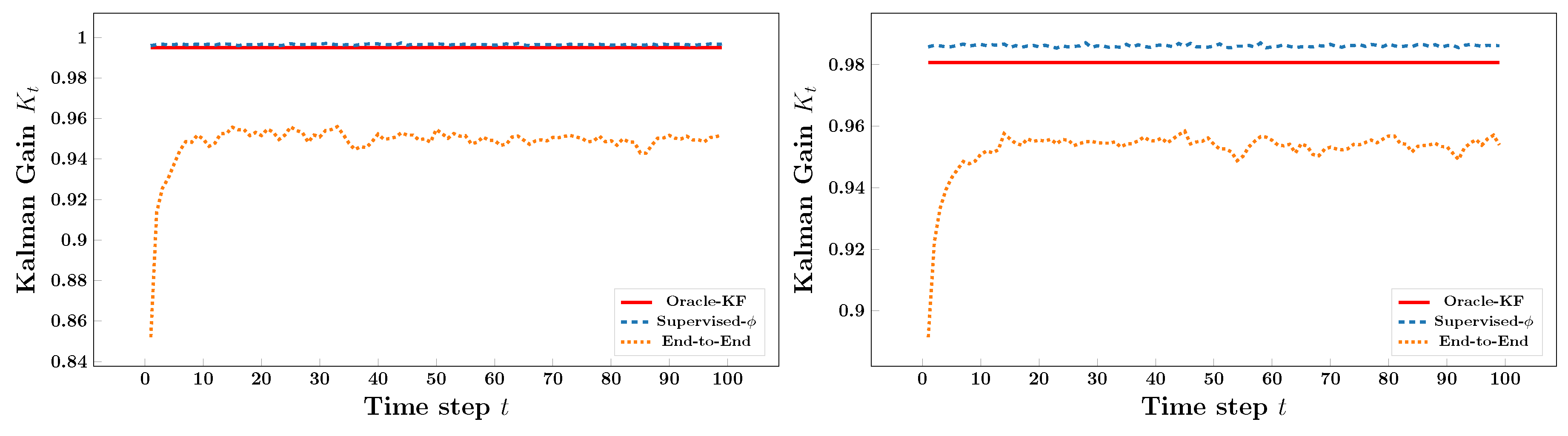
We simulate trajectories of length with fixed system parameters . To test robustness under different noise regimes, we consider four parameter settings by varying process noise Q and observation noise R: (i) ; (ii) ; (iii) ; (iv) . The supervised models are trained for 200 epochs using Adam optimizer with a learning rate . Performance is evaluated by:
- MSE of Gain:, measuring how well the learned gain matches the oracle trajectory.
- State Estimation RMSE: Root-mean-square error between estimated and true state trajectories, where the state estimates are produced by running a Kalman update step with the learned , verifying that accurate gain learning improves filtering quality.

Table A1.
Quantitative Results of Kalman Gain Learning. Supervised- achieves orders-of-magnitude lower gain MSE and consistently better state estimation RMSE across all noise regimes compared to End-to-End learning, highlighting the critical role of explicitly modeling the innovation term in recovering accurate Kalman gain dynamics.
| (Q, R) | Supervised- | End-to-End | ||
|---|---|---|---|---|
| MSE | RMSE | MSE | RMSE | |
| (5, 0.1) | 0.317 | 0.368 | ||
| (5, 0.5) | 0.684 | 0.694 | ||
| (10, 0.1) | 0.216 | 0.341 | ||
| (100, 0.5) | 0.310 | 0.747 | ||
- Results and Analysis
Figure A1 presents the learned Kalman gain trajectories across all considered noise regimes. Across every configuration, the Supervised- model closely matches the oracle Kalman gain , producing stable and accurate trajectories throughout both transient and steady phases. In contrast, the End-to-End model produces a noisier and slightly biased gain curve, indicating that omitting the explicit innovation term fails to accurately capture the gain dynamics. This qualitative observation is quantitatively confirmed in Table A1: Supervised- achieves up to four orders-of-magnitude lower gain MSE and reduces state-estimation RMSE by under all noise settings. These results demonstrate that the innovation term is indeed sufficient for inferring the optimal Kalman gain and that explicitly modeling innovation-driven selectivity yields more stable and accurate state estimation. Together, the figure and table provide strong empirical support for our theoretical claim that innovation-guided gain learning constitutes a principled and robust mechanism for selective state updates.
Figure A1.
Kalman gain learning across different noise regimes. Top-left: ; top-right: ; bottom-left: ; bottom-right: . Supervised- closely matches the oracle in all cases, while End-to-End trajectories remain noisy and biased. These results confirm that innovation-driven modeling provides stable and accurate gain learning across both low- and high-noise conditions.
Appendix C. SSR Case Study: Data and Preprocessing Details
Appendix C.1. Data Acquisition
The semi-physical training dataset is constructed using ADS-B logs from the OpenSky Network, recorded on June 15, 2025, between 10:00 and 10:15 AM. The data cover a 300 km region surrounding Tokyo Haneda, Narita, and Incheon Airports. Each log provides updates every 5 seconds for 503 aircraft, including longitude, latitude, altitude, and timestamp information. A detailed statistical summary of the dataset is provided in Table A2.
To emulate realistic Secondary Surveillance Radar (SSR) observation noise, zero-mean Gaussian perturbations are applied to each measurement with a signal-to-noise ratio (SNR) of 33 dB, formulated as
where represents the empirical variance of the i-th feature. This noise configuration reflects typical radar tracking uncertainty under moderate atmospheric interference.
Table A2.
Summary of the Semi-physical ADS-B Dataset Used for Training. The dataset consists of 5-second updates for 503 aircraft collected within a 15-minute window around major East Asian airports. Each sample includes four state variables: longitude, latitude, altitude, and timestamp.
Table A2.
Summary of the Semi-physical ADS-B Dataset Used for Training. The dataset consists of 5-second updates for 503 aircraft collected within a 15-minute window around major East Asian airports. Each sample includes four state variables: longitude, latitude, altitude, and timestamp.
| Targets | Update Frequency | # Features | Total Samples | Time Span |
|---|---|---|---|---|
| 503 | 5 seconds | 4 | 166,110 | 2025–06–15, 10:00–10:15 |
Appendix C.2. Normalization and Reverse Transformation
All input data are standardized to zero mean and unit variance:
Appendix C.3. Field Data Collection
For real-world evaluation, we use raw SSR plots collected by a field-deployed radar with a peak transmit power of 6 kW. These sequences contain irregular sampling, strong noise, and missing returns, providing a rigorous test of model robustness.
Figure A2.
SSR Trajectory Modeling Pipeline. The upper branch shows training using ADS-B data with noise simulation and normalization; the lower branch shows testing on real raw SSR plots using trained models, followed by trajectory prediction and comparison.
Figure A2.
SSR Trajectory Modeling Pipeline. The upper branch shows training using ADS-B data with noise simulation and normalization; the lower branch shows testing on real raw SSR plots using trained models, followed by trajectory prediction and comparison.
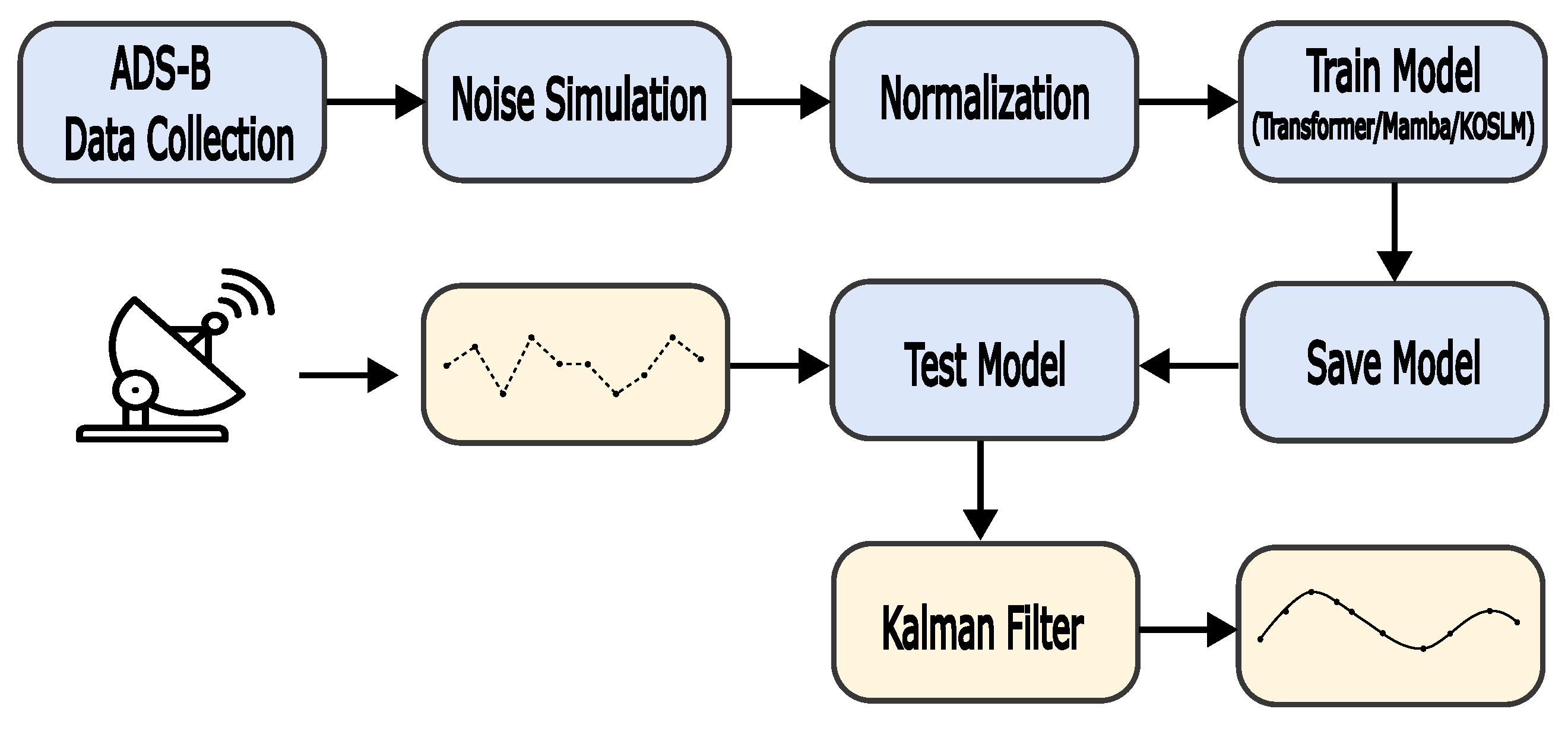
Appendix C.4. Processing Workflow
The overall pipeline—from semi-physical data generation to field testing—is summarized in Figure A2, where the upper branch denotes the training stage on noisy ADS-B data, and the lower branch represents inference on real SSR plots. This workflow ensures consistency between semi-physical training data and real-world SSR testing scenarios.
References
- Cheng, M.; Liu, Z.; Tao, X.; Liu, Q.; Zhang, J.; Pan, T.; Zhang, S.; He, P.; Zhang, X.; Wang, D.; et al. A comprehensive survey of time series forecasting: Concepts, challenges, and future directions. Authorea Preprints 2025.
- Salazar, C.; Banerjee, A.G. A distance correlation-based approach to characterize the effectiveness of recurrent neural networks for time series forecasting. Neurocomputing 2025, 629, 129641. [CrossRef]
- Hochreiter, S.; Schmidhuber, J. Long short-term memory. Neural computation 1997, 9, 1735–1780.
- Benjamin, J.; Mathew, J. Enhancing continuous integration predictions: a hybrid LSTM-GRU deep learning framework with evolved DBSO algorithm. Computing 2025, 107, 9. [CrossRef]
- Pascanu, R.; Mikolov, T.; Bengio, Y. On the Difficulty of Training Recurrent Neural Networks. In Proceedings of the Proceedings of the 30th International Conference on Machine Learning (ICML), Atlanta, GA, USA, 2013; ICML’13, pp. 1310–1318.
- Kalman, R.E. A New Approach to Linear Filtering and Prediction Problems. Journal of Basic Engineering 1960, 82, 35–45. [CrossRef]
- Yuan, X.; Li, J.; Kuruoglu, E.E. Robustness enhancement in neural networks with alpha-stable training noise. Digital Signal Processing 2025, 156, 104778. [CrossRef]
- Krishnan, R.G.; Shalit, U.; Sontag, D. Deep kalman filters. arXiv preprint arXiv:1511.05121 2015.
- Revach, G.; Shlezinger, N.; Ni, X.; Escoriza, A.L.; Van Sloun, R.J.; Eldar, Y.C. KalmanNet: Neural network aided Kalman filtering for partially known dynamics. IEEE Transactions on Signal Processing 2022, 70, 1532–1547. [CrossRef]
- Dahan, Y.; Revach, G.; Dunik, J.; Shlezinger, N. Uncertainty quantification in deep learning based Kalman filters. In Proceedings of the ICASSP 2024-2024 IEEE International Conference on Acoustics, Speech and Signal Processing (ICASSP). IEEE, 2024, pp. 13121–13125.
- Gu, A.; Dao, T. Mamba: Linear-time sequence modeling with selective state spaces. arXiv preprint arXiv:2312.00752 2023.
- Dao, T.; Gu, A. Transformers are ssms: Generalized models and efficient algorithms through structured state space duality. arXiv preprint arXiv:2405.21060 2024.
- Aliyu, B.K.; Osheku, C.A.; Adetoro, L.M.; Funmilayo, A.A. Optimal Solution to Matrix Riccati Equation – For Kalman Filter Implementation. In MATLAB; Katsikis, V.N., Ed.; IntechOpen: Rijeka, 2012; chapter 4. https://doi.org/10.5772/46456. [CrossRef]
- Gu, A.; Goel, K.; Gupta, A.; Ré, C. On the parameterization and initialization of diagonal state space models. Advances in Neural Information Processing Systems 2022, 35, 35971–35983.
- Gu, A.; Gulcehre, C.; Paine, T.; Hoffman, M.; Pascanu, R. Improving the gating mechanism of recurrent neural networks. In Proceedings of the International conference on machine learning. PMLR, 2020, pp. 3800–3809.
- Weather Dataset. Accessed: May 12, 2024. [Online], 2024. Weather data from the BGC Jena Climate Data archive.
- ETT Datasets. Accessed: May 12, 2024. [Online], 2024. Energy Transformer Temperature dataset (ETT) for long-term forecasting.
- Electricity Dataset. Accessed: May 12, 2024. [Online], 2024. Electricity load diagrams dataset from UCI Machine Learning Repository.
- Exchange Rate Dataset. Accessed: May 12, 2024. [Online], 2024. Daily exchange rate dataset for long-term time series forecasting, provided with the ETT benchmark collection.
- Traffic Dataset. Accessed: May 12, 2024. [Online], 2024. Traffic flow data from California Performance Measurement System (PeMS).
- Illness (ILI) Dataset. Accessed: May 12, 2024. [Online], 2024. Weekly influenza-like illness (ILI) dataset for forecasting tasks, available within the ETT benchmark suite.
- Alharthi, M.; Mahmood, A. xlstmtime: Long-term time series forecasting with xlstm. AI 2024, 5, 1482–1495. [CrossRef]
- Zhou, T.; Ma, Z.; Wen, Q.; Sun, L.; Yao, T.; Yin, W.; Jin, R.; et al. Film: Frequency improved legendre memory model for long-term time series forecasting. Advances in neural information processing systems 2022, 35, 12677–12690.
- Wang, Z.; Kong, F.; Feng, S.; Wang, M.; Yang, X.; Zhao, H.; Wang, D.; Zhang, Y. Is mamba effective for time series forecasting? Neurocomputing 2025, 619, 129178. [CrossRef]
- Zhou, T.; Ma, Z.; Wen, Q.; Wang, X.; Sun, L.; Jin, R. Fedformer: Frequency enhanced decomposed transformer for long-term series forecasting. In Proceedings of the International conference on machine learning. PMLR, 2022, pp. 27268–27286.
- Liu, Y.; Hu, T.; Zhang, H.; Wu, H.; Wang, S.; Ma, L.; Long, M. itransformer: Inverted transformers are effective for time series forecasting. arXiv preprint arXiv:2310.06625 2023.
- Zhang, Y.; Yan, J. Crossformer: Transformer Utilizing Cross-Dimension Dependency for Multivariate Time Series Forecasting. In Proceedings of the Proceedings of the Eleventh International Conference on Learning Representations (ICLR), 2023. OpenReview preprint.
- Su, J.; Shen, Y.; Wu, Z.; et al.. DLinear: A Linear Complexity Approach for Long-Term Time Series Forecasting. arXiv preprint arXiv:2205.13504 2022.
- Huang, X.; Tang, J.; Shen, Y. Long time series of ocean wave prediction based on PatchTST model. Ocean Engineering 2024, 301, 117572. [CrossRef]
- Wang, S.; Wu, H.; Shi, X.; Hu, T.; Luo, H.; Ma, L.; Zhang, J.Y.; Zhou, J. Timemixer: Decomposable multiscale mixing for time series forecasting. arXiv preprint arXiv:2405.14616 2024.
- Dao, T. Flashattention-2: Faster attention with better parallelism and work partitioning. arXiv preprint arXiv:2307.08691 2024.
- Zhang, J.; Wei, L.; Yanbo, Z. Study of ADS-B data evaluation. Chinese Journal of Aeronautics 2011, 24, 461–466.
- Cho, K.; Van Merriënboer, B.; Gulcehre, C.; Bahdanau, D.; Bougares, F.; Schwenk, H.; Bengio, Y. Learning phrase representations using RNN encoder-decoder for statistical machine translation. In Proceedings of the EMNLP, 2014, pp. 1724–1734.
- Mehta, H.; Gupta, A.; Cutkosky, A.; Neyshabur, B. Long range language modeling via gated state spaces. arXiv preprint arXiv:2206.13947 2022.
- Hua, W.; Dai, Z.; Liu, H.; Le, Q. Transformer quality in linear time. In Proceedings of the International conference on machine learning. PMLR, 2022, pp. 9099–9117.
- Ha, D.; Dai, A.; Le, Q.V. Hypernetworks. arXiv preprint arXiv:1609.09106 2016.
- Poli, M.; et al. Data-dependent neural networks. arXiv preprint arXiv:2305.13272 2023.
- Gu, A.; Goel, K.; Ré, C. Combining recurrent, convolutional, and continuous-time models with structured state space. Advances in Neural Information Processing Systems 2021, 34, 21984–21998.
- Funahashi, K.I.; Nakamura, Y. Approximation of dynamical systems by continuous time recurrent neural networks. Neural networks 1993, 6, 801–806. [CrossRef]
- Tallec, C.; Ollivier, Y. Can recurrent neural networks warp time? arXiv preprint arXiv:1804.11188 2018.
- Tahirovic, A.; Redzovic, A. Optimal Estimation for Continuous-Time Nonlinear Systems Using State-Dependent Riccati Equation (SDRE). arXiv preprint arXiv:2503.10442 2025.
| 1 | Here, the observation input denotes the externally observable signal that directly drives the state update process. It is written as in KF and as in SSMs, which are semantically equivalent. |
Figure 1.
Structure of the LSTM network.
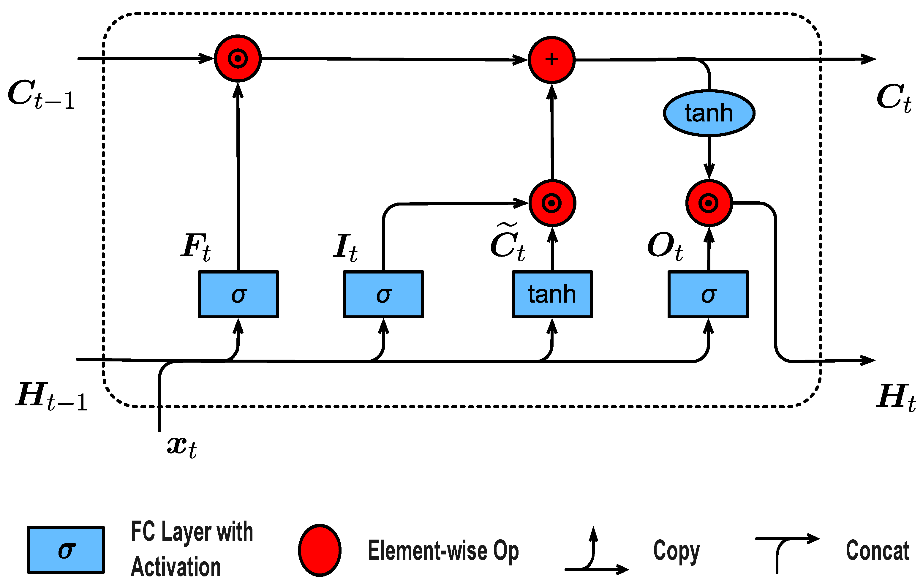
Figure 2.
Unfolded KOSLM network layer. The D-dimensional input is dynamically coupled with the N-dimensional hidden state and mapped to the output through the higher-dimensional cell state . Compared to the heuristic forget and output gates of the classical LSTM, our mechanism introduces Kalman-optimal constraints by parameterizing SSM parameters (, ) based on the innovation term.
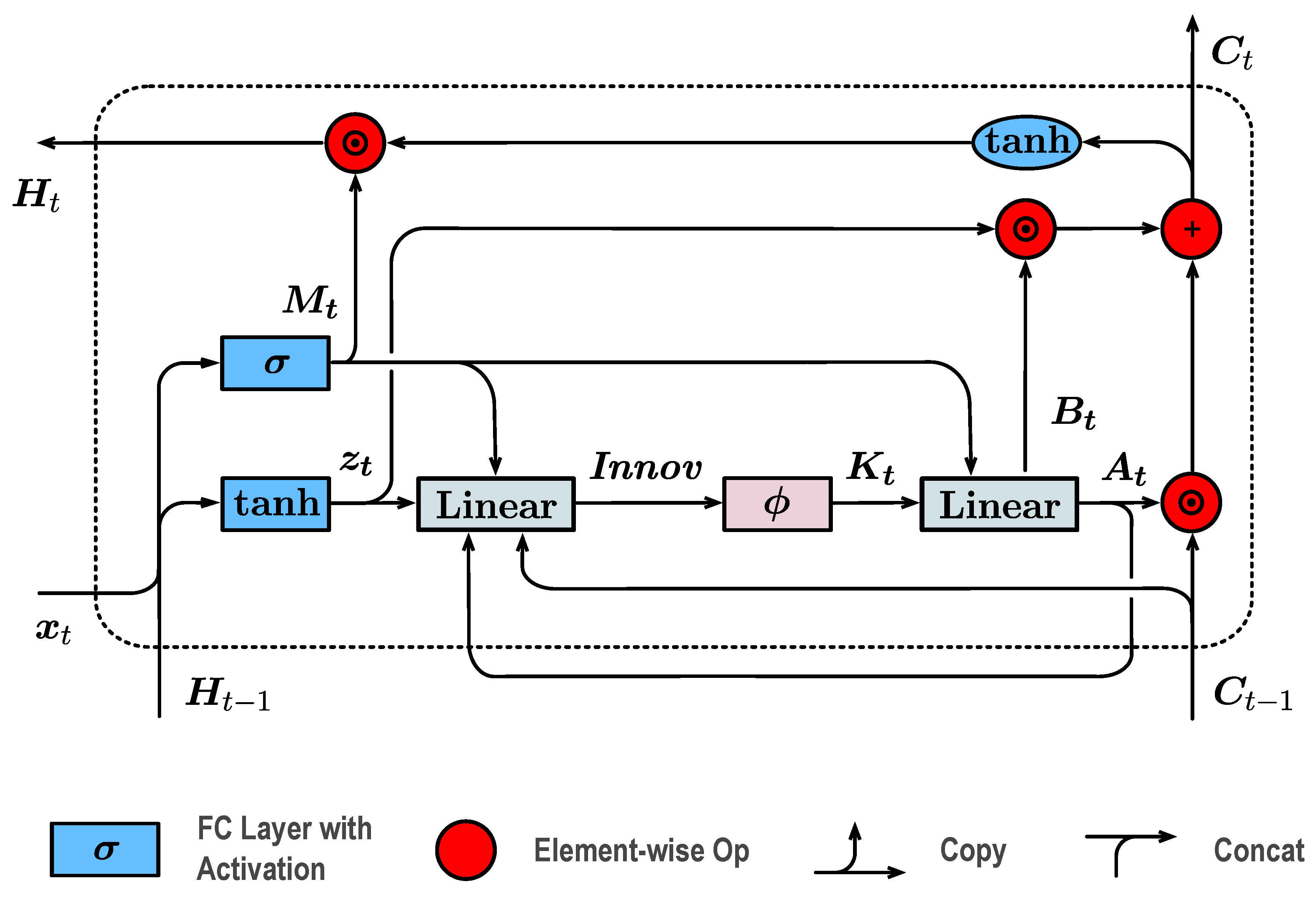
Figure 3.
KOSLM vs. S-Mamba: Forecasting comparison on five representative datasets with both input and prediction horizons set to 720. The blue line denotes the ground truth, and the red line indicates model predictions. KOSLM demonstrates superior long-horizon stability and trend consistency compared to S-Mamba.
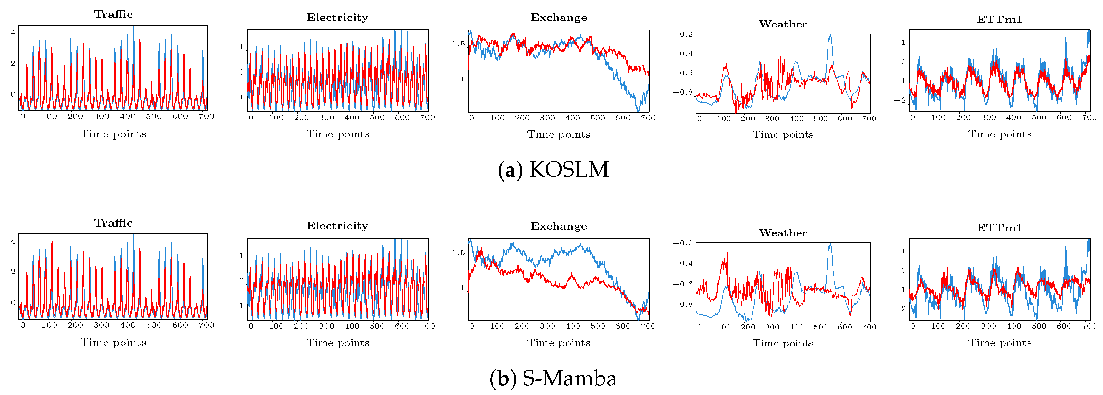
Figure 4.
Runtime Benchmarks. Inference time (ms) as a function of sequence length L. KOSLM demonstrates near-linear scaling and maintains faster inference than Transformer and Mamba-2 for long sequences.
Figure 4.
Runtime Benchmarks. Inference time (ms) as a function of sequence length L. KOSLM demonstrates near-linear scaling and maintains faster inference than Transformer and Mamba-2 for long sequences.
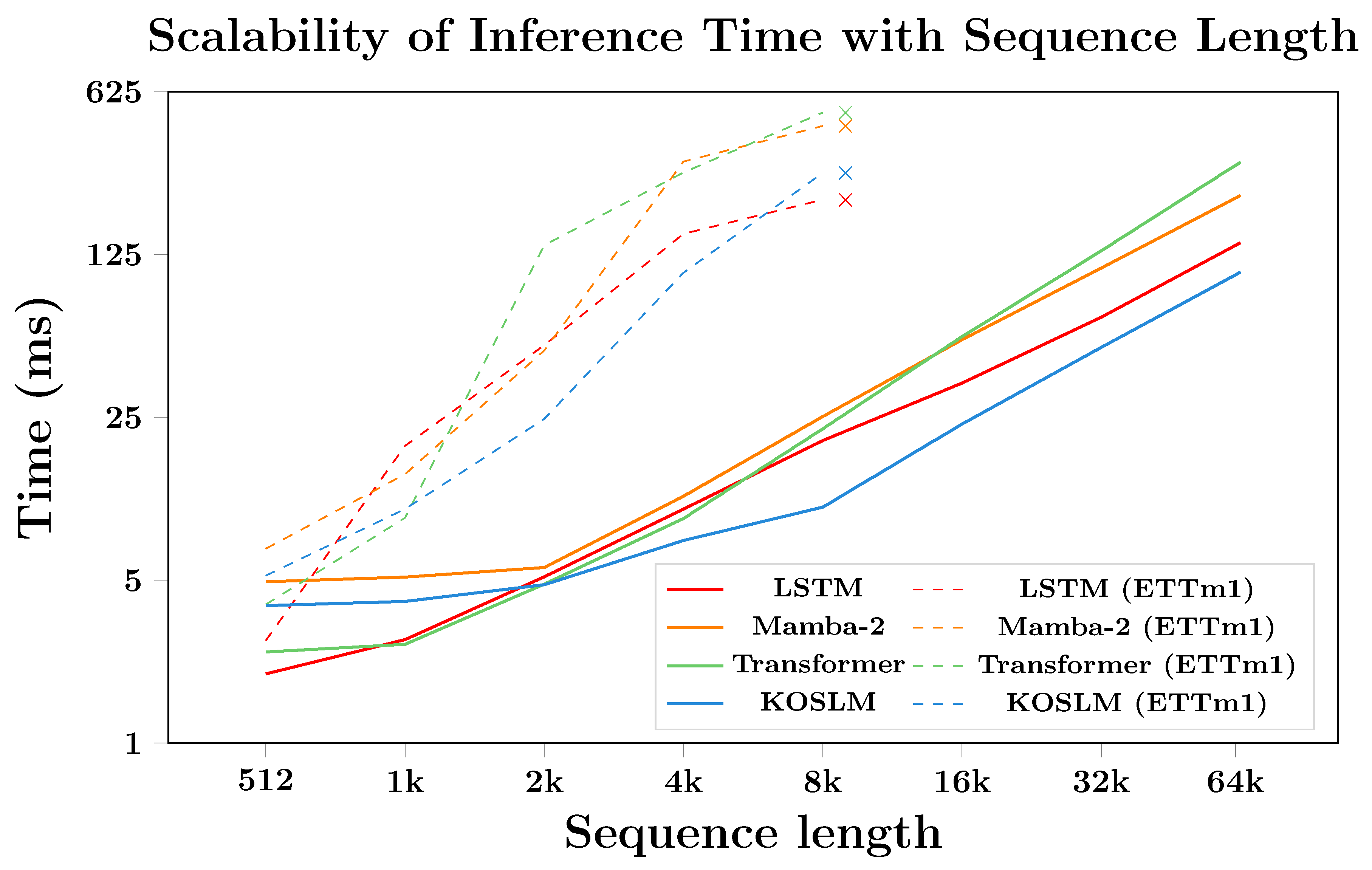
Figure 5.
Throughput Benchmarks. End-to-end inference throughput on RTX 4090. KOSLM maintains stable throughput as sequence length increases, outperforming LSTM and Mamba-2 for long sequences.
Figure 5.
Throughput Benchmarks. End-to-end inference throughput on RTX 4090. KOSLM maintains stable throughput as sequence length increases, outperforming LSTM and Mamba-2 for long sequences.
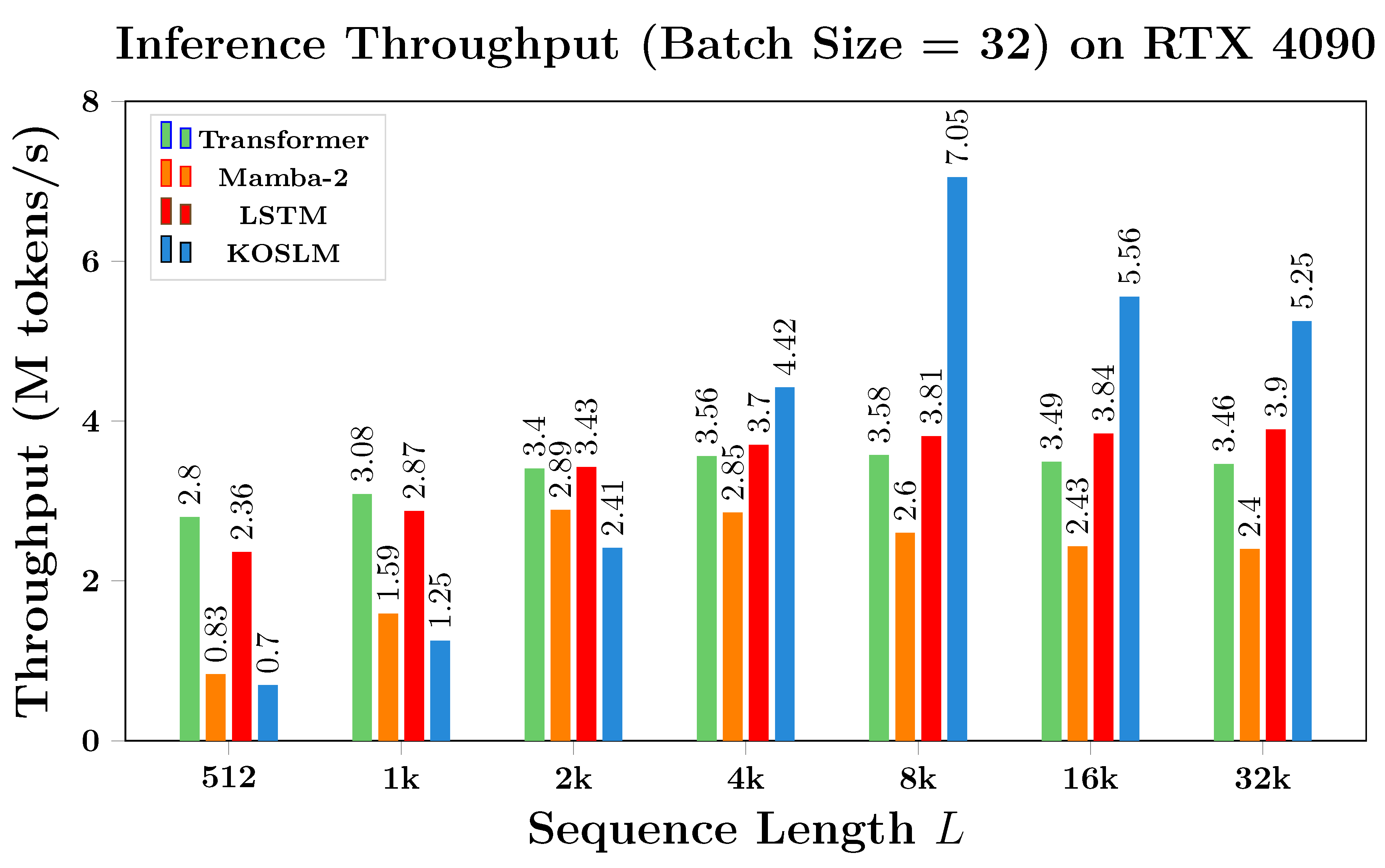
Figure 6.
SSR Target Tracking under Real-world Operational Conditions. Trajectories of eight air-traffic targets tracked from SSR measurements. Red curves denote raw SSR observations, Blue curves denote tracking by the conventional KF algorithm (on-site SSR interrogator output), and Teal curves indicate deep model predictions (Transformer, Mamba, or KOSLM), followed by KF smoothing. KOSLM achieves smoother, more accurate, and stable tracking under strong noise and irregular sampling conditions.
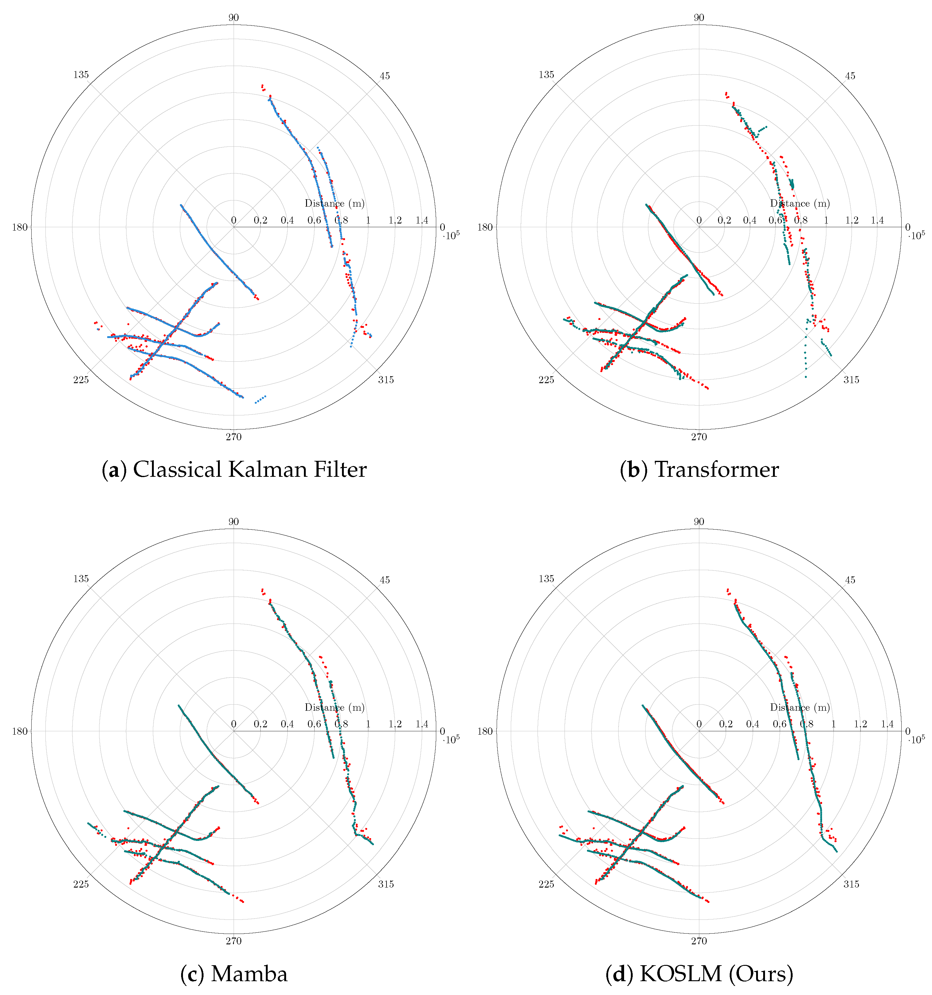
Table 1.
Core Structural Comparison between KalmanNet and KOSLM.
| Aspect | KalmanNet | KOSLM (Ours) |
|---|---|---|
| Core idea | Strictly follows the classical KF architecture (§Section 2.2.2); the neural network learns to correct the Kalman gain under partially known linear dynamics. | Reinterprets LSTM gating as a Kalman-optimal state estimation problem; state estimation does not strictly adhere to the KF equations, but directly learns from the innovation term. |
| System dynamics | Assumes fixed parameters ; suitable for systems with known or partially known dynamics. | Learns from data; A is a learnable parameter matrix; fully adaptive to nonlinear and nonstationary environments. |
| Form of gain | — learns a residual correction to the classical Kalman gain. | — directly learns the gain function from the innovation. |
| Gain network input | — uses both predicted state and innovation as inputs. | — relies solely on the innovation signal for gain computation (see Appendices Appendix B.3 and Appendix B.4, which prove its sufficiency). |
| Output role | Outputs a residual correction added to . | Outputs and integrates gain estimation into the state transition: , , forming a unified recurrent–estimation pathway. |
| System dependency | Requires partial knowledge of for baseline Kalman computation. | Fully data-driven; no analytical Kalman gain or explicit system parameters required. |
| Theoretical interpretation | Neural residual learning to compensate model mismatch. | Innovation-driven dynamic selectivity that enforces Kalman-optimal information update behavior. |
Table 2.
Details of benchmark datasets used in our experiments.
| Dataset | Frequency | # Features | Time Steps | Time Span |
|---|---|---|---|---|
| ETTh1 | 1 hour | 7 | 17,420 | 2016–2017 |
| ETTh2 | 1 hour | 7 | 17,420 | 2017–2018 |
| ETTm1 | 15 minutes | 7 | 69,680 | 2016–2017 |
| ETTm2 | 15 minutes | 7 | 69,680 | 2017–2018 |
| Exchange | 1 day | 8 | 7,588 | 1990–2010 |
| Weather | 10 minutes | 21 | 52,696 | 2020 |
| Electricity | 1 hour | 321 | 26,304 | 2012–2014 |
| ILI | 7 days | 7 | 966 | 2002–2020 |
| Traffic | 1 hour | 862 | 17,544 | 2015–2016 |
Table 3.
Long-Term Forecasting: Multivariate long-term forecasting results on the Traffic, Electricity, Exchange, Weather, and ILI datasets. The prediction length is set to for all datasets except ILI, which uses due to its weekly resolution. The best results are shown in bold red, and the second-best are underlined purple. All results are averaged over 5 runs.
| Models | KOSLM | xLSTMTime | FiLM | iTransformer | FEDFormer | S-Mamba | Crossformer | DLinear | PatchTST | TimeMixer | |||||||||||
|---|---|---|---|---|---|---|---|---|---|---|---|---|---|---|---|---|---|---|---|---|---|
| Metric | MSE | MAE | MSE | MAE | MSE | MAE | MSE | MAE | MSE | MAE | MSE | MAE | MSE | MAE | MSE | MAE | MSE | MAE | MSE | MAE | |
| Traffic | 96 | 0.290 | 0.230 | 0.358 | 0.242 | 0.416 | 0.294 | 0.395 | 0.268 | 0.587 | 0.366 | 0.382 | 0.261 | 0.522 | 0.290 | 0.650 | 0.396 | 0.462 | 0.295 | 0.462 | 0.285 |
| 192 | 0.260 | 0.210 | 0.378 | 0.253 | 0.408 | 0.288 | 0.417 | 0.276 | 0.604 | 0.373 | 0.396 | 0.267 | 0.530 | 0.293 | 0.598 | 0.370 | 0.466 | 0.296 | 0.473 | 0.296 | |
| 336 | 0.227 | 0.179 | 0.392 | 0.261 | 0.425 | 0.298 | 0.433 | 0.283 | 0.621 | 0.383 | 0.417 | 0.276 | 0.558 | 0.305 | 0.605 | 0.373 | 0.482 | 0.304 | 0.498 | 0.297 | |
| 720 | 0.290 | 0.232 | 0.434 | 0.287 | 0.520 | 0.353 | 0.467 | 0.302 | 0.626 | 0.382 | 0.460 | 0.300 | 0.589 | 0.328 | 0.645 | 0.394 | 0.514 | 0.322 | 0.506 | 0.313 | |
| +31.96% | Avg | 0.266 | 0.212 | 0.391 | 0.261 | 0.442 | 0.308 | 0.428 | 0.282 | 0.610 | 0.376 | 0.434 | 0.287 | 0.550 | 0.304 | 0.625 | 0.383 | 0.481 | 0.304 | 0.485 | 0.297 |
| Electricity | 96 | 0.136 | 0.184 | 0.128 | 0.221 | 0.154 | 0.267 | 0.148 | 0.240 | 0.193 | 0.308 | 0.139 | 0.235 | 0.219 | 0.314 | 0.197 | 0.282 | 0.181 | 0.270 | 0.153 | 0.247 |
| 192 | 0.131 | 0.184 | 0.150 | 0.243 | 0.164 | 0.258 | 0.162 | 0.253 | 0.201 | 0.315 | 0.159 | 0.255 | 0.231 | 0.322 | 0.196 | 0.285 | 0.188 | 0.274 | 0.166 | 0.256 | |
| 336 | 0.120 | 0.177 | 0.166 | 0.259 | 0.188 | 0.283 | 0.178 | 0.269 | 0.214 | 0.329 | 0.176 | 0.272 | 0.246 | 0.337 | 0.209 | 0.301 | 0.204 | 0.293 | 0.185 | 0.277 | |
| 720 | 0.158 | 0.205 | 0.185 | 0.276 | 0.236 | 0.332 | 0.225 | 0.317 | 0.246 | 0.355 | 0.204 | 0.298 | 0.280 | 0.363 | 0.245 | 0.333 | 0.246 | 0.324 | 0.225 | 0.310 | |
| +13.37% | Avg | 0.136 | 0.187 | 0.157 | 0.250 | 0.186 | 0.285 | 0.178 | 0.270 | 0.214 | 0.327 | 0.170 | 0.265 | 0.244 | 0.334 | 0.212 | 0.300 | 0.205 | 0.290 | 0.182 | 0.272 |
| Exchange | 96 | 0.135 | 0.212 | – | – | 0.086 | 0.204 | 0.086 | 0.206 | 0.148 | 0.278 | 0.086 | 0.207 | 0.256 | 0.367 | 0.088 | 0.218 | 0.088 | 0.205 | 0.095 | 0.207 |
| 192 | 0.279 | 0.292 | – | – | 0.188 | 0.292 | 0.177 | 0.299 | 0.271 | 0.315 | 0.182 | 0.304 | 0.470 | 0.509 | 0.176 | 0.315 | 0.176 | 0.299 | 0.151 | 0.293 | |
| 336 | 0.341 | 0.339 | – | – | 0.356 | 0.433 | 0.331 | 0.417 | 0.460 | 0.427 | 0.332 | 0.418 | 1.268 | 0.883 | 0.313 | 0.427 | 0.301 | 0.397 | 0.264 | 0.361 | |
| 720 | 0.282 | 0.322 | – | – | 0.727 | 0.669 | 0.847 | 0.691 | 1.195 | 0.695 | 0.867 | 0.703 | 1.767 | 1.068 | 0.839 | 0.695 | 0.901 | 0.714 | 0.586 | 0.602 | |
| +5.47% | Avg | 0.259 | 0.291 | – | – | 0.339 | 0.400 | 0.360 | 0.403 | 0.519 | 0.429 | 0.367 | 0.408 | 0.940 | 0.707 | 0.354 | 0.414 | 0.367 | 0.404 | 0.274 | 0.365 |
| Weather | 96 | 0.144 | 0.171 | 0.144 | 0.187 | 0.199 | 0.262 | 0.174 | 0.214 | 0.217 | 0.296 | 0.165 | 0.210 | 0.158 | 0.230 | 0.196 | 0.255 | 0.177 | 0.218 | 0.163 | 0.209 |
| 192 | 0.224 | 0.236 | 0.192 | 0.236 | 0.228 | 0.288 | 0.221 | 0.254 | 0.276 | 0.336 | 0.214 | 0.252 | 0.206 | 0.277 | 0.237 | 0.296 | 0.225 | 0.259 | 0.208 | 0.250 | |
| 336 | 0.249 | 0.248 | 0.237 | 0.272 | 0.267 | 0.323 | 0.278 | 0.296 | 0.339 | 0.380 | 0.274 | 0.297 | 0.272 | 0.335 | 0.283 | 0.335 | 0.278 | 0.297 | 0.251 | 0.287 | |
| 720 | 0.169 | 0.175 | 0.313 | 0.326 | 0.319 | 0.361 | 0.358 | 0.347 | 0.403 | 0.428 | 0.350 | 0.345 | 0.398 | 0.418 | 0.345 | 0.381 | 0.354 | 0.348 | 0.339 | 0.341 | |
| +11.26% | Avg | 0.197 | 0.208 | 0.222 | 0.255 | 0.253 | 0.309 | 0.258 | 0.278 | 0.309 | 0.360 | 0.251 | 0.276 | 0.259 | 0.315 | 0.265 | 0.317 | 0.259 | 0.281 | 0.240 | 0.271 |
| ILI | 24 | 1.160 | 0.507 | 1.514 | 0.694 | 1.970 | 0.875 | 3.154 | 1.235 | 3.228 | 1.260 | – | – | 3.041 | 1.186 | 2.215 | 1.081 | 1.319 | 0.754 | 1.453 | 0.827 |
| 36 | 1.262 | 0.561 | 1.519 | 0.722 | 1.982 | 0.859 | 2.544 | 1.083 | 2.679 | 1.150 | – | – | 3.406 | 1.232 | 1.963 | 0.963 | 1.579 | 0.870 | 1.627 | 0.903 | |
| 48 | 1.098 | 0.545 | 1.500 | 0.725 | 1.868 | 0.896 | 2.489 | 1.112 | 2.622 | 1.080 | – | – | 3.459 | 1.221 | 2.130 | 1.024 | 1.553 | 0.815 | 1.644 | 0.914 | |
| 60 | 1.118 | 0.583 | 1.418 | 0.715 | 2.057 | 0.929 | 2.675 | 1.034 | 2.857 | 1.078 | – | – | 3.640 | 1.305 | 2.368 | 1.096 | 1.470 | 0.788 | 1.633 | 0.908 | |
| +22.04% | Avg | 1.160 | 0.549 | 1.488 | 0.714 | 1.969 | 0.890 | 2.715 | 1.116 | 2.847 | 1.170 | – | – | 3.387 | 1.236 | 2.169 | 1.041 | 1.480 | 0.807 | 1.589 | 0.888 |
Table 4.
Long-Term Forecasting: Forecasting results on the ETT datasets with prediction lengths . The best results are shown in bold red, and the second-best are underlined purple. All results are averaged over 5 runs.
Table 4.
Long-Term Forecasting: Forecasting results on the ETT datasets with prediction lengths . The best results are shown in bold red, and the second-best are underlined purple. All results are averaged over 5 runs.
| Models | KOSLM | xLSTMTime | FiLM | iTransformer | FEDFormer | S-Mamba | Crossformer | DLinear | PatchTST | TimeMixer | |||||||||||
|---|---|---|---|---|---|---|---|---|---|---|---|---|---|---|---|---|---|---|---|---|---|
| Metric | MSE | MAE | MSE | MAE | MSE | MAE | MSE | MAE | MSE | MAE | MSE | MAE | MSE | MAE | MSE | MAE | MSE | MAE | MSE | MAE | |
| ETTm1 | 96 | 0.204 | 0.221 | 0.286 | 0.335 | – | – | 0.334 | 0.368 | 0.379 | 0.419 | 0.333 | 0.368 | 0.404 | 0.426 | 0.345 | 0.372 | 0.329 | 0.367 | 0.320 | 0.357 |
| 192 | 0.233 | 0.237 | 0.329 | 0.361 | – | – | 0.377 | 0.391 | 0.426 | 0.441 | 0.376 | 0.390 | 0.450 | 0.451 | 0.380 | 0.389 | 0.367 | 0.385 | 0.361 | 0.381 | |
| 336 | 0.414 | 0.339 | 0.358 | 0.379 | – | – | 0.426 | 0.420 | 0.445 | 0.459 | 0.408 | 0.413 | 0.532 | 0.515 | 0.413 | 0.413 | 0.399 | 0.410 | 0.390 | 0.404 | |
| 720 | 0.481 | 0.368 | 0.416 | 0.411 | – | – | 0.491 | 0.459 | 0.543 | 0.490 | 0.475 | 0.448 | 0.666 | 0.589 | 0.474 | 0.453 | 0.454 | 0.439 | 0.458 | 0.441 | |
| +4.03% | Avg | 0.333 | 0.291 | 0.347 | 0.372 | – | – | 0.407 | 0.410 | 0.448 | 0.452 | 0.398 | 0.405 | 0.513 | 0.496 | 0.403 | 0.407 | 0.387 | 0.400 | 0.382 | 0.395 |
| ETTm2 | 96 | 0.100 | 0.232 | 0.164 | 0.250 | 0.165 | 0.256 | 0.180 | 0.264 | 0.203 | 0.287 | 0.179 | 0.263 | 0.287 | 0.366 | 0.193 | 0.292 | 0.175 | 0.259 | 0.175 | 0.258 |
| 192 | 0.132 | 0.274 | 0.218 | 0.288 | 0.222 | 0.296 | 0.250 | 0.309 | 0.269 | 0.328 | 0.250 | 0.309 | 0.414 | 0.492 | 0.284 | 0.362 | 0.241 | 0.302 | 0.237 | 0.299 | |
| 336 | 0.244 | 0.382 | 0.271 | 0.322 | 0.277 | 0.333 | 0.311 | 0.348 | 0.325 | 0.366 | 0.312 | 0.349 | 0.597 | 0.542 | 0.369 | 0.427 | 0.305 | 0.343 | 0.298 | 0.340 | |
| 720 | 0.268 | 0.408 | 0.361 | 0.380 | 0.371 | 0.389 | 0.412 | 0.407 | 0.421 | 0.415 | 0.411 | 0.406 | 1.730 | 1.042 | 0.554 | 0.522 | 0.402 | 0.400 | 0.275 | 0.323 | |
| +24.39% | Avg | 0.186 | 0.324 | 0.254 | 0.310 | 0.259 | 0.319 | 0.288 | 0.332 | 0.305 | 0.349 | 0.288 | 0.332 | 0.757 | 0.610 | 0.350 | 0.401 | 0.281 | 0.326 | 0.246 | 0.306 |
| ETTh1 | 96 | 0.298 | 0.277 | 0.368 | 0.395 | – | – | 0.386 | 0.405 | 0.376 | 0.419 | 0.386 | 0.405 | 0.423 | 0.448 | 0.386 | 0.400 | 0.414 | 0.419 | 0.375 | 0.400 |
| 192 | 0.337 | 0.306 | 0.401 | 0.416 | – | – | 0.441 | 0.436 | 0.420 | 0.448 | 0.443 | 0.437 | 0.471 | 0.474 | 0.437 | 0.432 | 0.460 | 0.445 | 0.479 | 0.421 | |
| 336 | 0.395 | 0.334 | 0.422 | 0.437 | – | – | 0.487 | 0.458 | 0.459 | 0.465 | 0.489 | 0.468 | 0.570 | 0.546 | 0.481 | 0.459 | 0.501 | 0.466 | 0.484 | 0.458 | |
| 720 | 0.471 | 0.364 | 0.441 | 0.465 | – | – | 0.503 | 0.491 | 0.506 | 0.507 | 0.502 | 0.489 | 0.653 | 0.621 | 0.519 | 0.516 | 0.500 | 0.488 | 0.498 | 0.482 | |
| +8.09% | Avg | 0.375 | 0.320 | 0.408 | 0.428 | – | – | 0.454 | 0.447 | 0.440 | 0.460 | 0.455 | 0.450 | 0.529 | 0.522 | 0.456 | 0.452 | 0.469 | 0.454 | 0.459 | 0.440 |
| ETTh2 | 96 | 0.194 | 0.338 | 0.273 | 0.333 | – | – | 0.297 | 0.349 | 0.358 | 0.397 | 0.296 | 0.348 | 0.745 | 0.584 | 0.333 | 0.387 | 0.302 | 0.348 | 0.289 | 0.341 |
| 192 | 0.238 | 0.384 | 0.340 | 0.378 | – | – | 0.380 | 0.400 | 0.429 | 0.439 | 0.376 | 0.396 | 0.877 | 0.656 | 0.477 | 0.476 | 0.388 | 0.400 | 0.372 | 0.392 | |
| 336 | 0.258 | 0.394 | 0.373 | 0.403 | – | – | 0.428 | 0.432 | 0.496 | 0.487 | 0.424 | 0.431 | 1.043 | 0.731 | 0.594 | 0.541 | 0.426 | 0.433 | 0.386 | 0.414 | |
| 720 | 0.314 | 0.432 | 0.398 | 0.430 | – | – | 0.427 | 0.445 | 0.463 | 0.474 | 0.426 | 0.444 | 1.104 | 0.763 | 0.831 | 0.657 | 0.431 | 0.446 | 0.412 | 0.434 | |
| +27.46% | Avg | 0.251 | 0.387 | 0.346 | 0.386 | – | – | 0.383 | 0.407 | 0.437 | 0.449 | 0.381 | 0.405 | 0.942 | 0.684 | 0.559 | 0.515 | 0.387 | 0.407 | 0.364 | 0.395 |
Table 5.
Structural Ablation. Comparison of KOSLM and its structural variants on four long-term forecasting datasets (). Removing either the Kalman gain path or the innovation input leads to consistent performance degradation. All results are averaged over five runs with mean ± standard deviation. Lower is better.
| Dataset | Model | MSE ↓ | MAE ↓ | MSE vs Full |
|---|---|---|---|---|
| ETTm1 | Full | 0.498 ± 0.011 | 0.416 ± 0.007 | — |
| No-Gain | 0.662 ± 0.017 | 0.553 ± 0.014 | +32.9% | |
| No-Innov | 0.583 ± 0.012 | 0.487 ± 0.008 | +17.1% | |
| ETTh1 | Full | 0.510 ± 0.012 | 0.378 ± 0.010 | — |
| No-Gain | 0.605 ± 0.022 | 0.448 ± 0.015 | +18.6% | |
| No-Innov | 0.554 ± 0.016 | 0.411 ± 0.010 | +8.6% | |
| Traffic | Full | 0.321 ± 0.008 | 0.195 ± 0.016 | — |
| No-Gain | 0.428 ± 0.011 | 0.260 ± 0.008 | +33.4% | |
| No-Innov | 0.375 ± 0.009 | 0.228 ± 0.007 | +16.9% | |
| Exchange | Full | 0.266 ± 0.014 | 0.341 ± 0.023 | — |
| No-Gain | 0.299 ± 0.018 | 0.383 ± 0.023 | +12.3% | |
| No-Innov | 0.294 ± 0.015 | 0.377 ± 0.019 | +10.6% |
Table 6.
Capacity Ablation (Corrected). Performance of KOSLM with varying network capacities on four long-term forecasting datasets (). Averaged over five runs with standard deviations. Bold font highlights the variant under comparison.
Table 6.
Capacity Ablation (Corrected). Performance of KOSLM with varying network capacities on four long-term forecasting datasets (). Averaged over five runs with standard deviations. Bold font highlights the variant under comparison.
| Dataset | Variant | #Params | MSE ↓ | MAE ↓ | MSE vs SmallMLP |
|---|---|---|---|---|---|
| ETTm1 | Linear | 0.183M | 0.480 ± 0.012 | 0.355 ± 0.008 | +46.3% |
| SmallMLP | 0.255M | 0.328 ± 0.010 | 0.282 ± 0.007 | — | |
| MediumMLP | 0.389M | 0.335 ± 0.011 | 0.284 ± 0.001 | +2.13% | |
| HighCap | 0.898M | 0.342 ± 0.015 | 0.288 ± 0.010 | +4.27% | |
| ETTh1 | Linear | 0.183M | 0.440 ± 0.010 | 0.330 ± 0.004 | +30.95% |
| SmallMLP | 0.255M | 0.336 ± 0.008 | 0.291 ± 0.006 | — | |
| MediumMLP | 0.389M | 0.341 ± 0.010 | 0.294 ± 0.002 | +1.49% | |
| HighCap | 0.898M | 0.355 ± 0.012 | 0.302 ± 0.008 | +5.65% | |
| Traffic | Linear | 0.183M | 0.290 ± 0.011 | 0.232 ± 0.006 | +9.02% |
| SmallMLP | 0.255M | 0.266 ± 0.010 | 0.212 ± 0.007 | — | |
| MediumMLP | 0.389M | 0.270 ± 0.012 | 0.216 ± 0.002 | +1.50% | |
| HighCap | 0.898M | 0.279 ± 0.014 | 0.222 ± 0.005 | +4.89% | |
| Exchange | Linear | 0.183M | 0.272 ± 0.010 | 0.305 ± 0.005 | +4.62% |
| SmallMLP | 0.255M | 0.260 ± 0.009 | 0.291 ± 0.009 | — | |
| MediumMLP | 0.389M | 0.264 ± 0.010 | 0.294 ± 0.007 | +1.54% | |
| HighCap | 0.898M | 0.285 ± 0.012 | 0.310 ± 0.009 | +9.62% |
Table 7.
Memory Footprint (GB) under Different Batch Sizes, Input Length = 2048. KOSLM exhibits lower memory usage than Transformer and Mamba-2, while remaining comparable to LSTM despite its smaller size.
Table 7.
Memory Footprint (GB) under Different Batch Sizes, Input Length = 2048. KOSLM exhibits lower memory usage than Transformer and Mamba-2, while remaining comparable to LSTM despite its smaller size.
| Batch Size | Transformer | Mamba-2 | LSTM | KOSLM |
|---|---|---|---|---|
| 1 | 0.223 | 0.085 | 0.081 | 0.061 |
| 2 | 0.363 | 0.158 | 0.109 | 0.104 |
| 4 | 0.640 | 0.290 | 0.166 | 0.188 |
| 8 | 1.180 | 0.561 | 0.283 | 0.344 |
| 16 | 2.256 | 1.103 | 0.518 | 0.668 |
| 32 | 4.408 | 2.188 | 0.987 | 1.317 |
| 64 | 8.712 | 4.357 | 1.926 | 2.615 |
| 128 | 17.000 | 8.696 | 3.803 | 5.211 |
Table 8.
Model Parameter Sizes. KOSLM remains lightweight while providing competitive long-horizon forecasting performance.
Table 8.
Model Parameter Sizes. KOSLM remains lightweight while providing competitive long-horizon forecasting performance.
| Model | Parameters (M) |
|---|---|
| LSTM | 2.17 |
| Transformer | 5.33 |
| Mamba-2 | 0.21 |
| FiLM | 1.50 |
| KOSLM | 0.24 |
Disclaimer/Publisher’s Note: The statements, opinions and data contained in all publications are solely those of the individual author(s) and contributor(s) and not of MDPI and/or the editor(s). MDPI and/or the editor(s) disclaim responsibility for any injury to people or property resulting from any ideas, methods, instructions or products referred to in the content. |
© 2025 by the authors. Licensee MDPI, Basel, Switzerland. This article is an open access article distributed under the terms and conditions of the Creative Commons Attribution (CC BY) license (http://creativecommons.org/licenses/by/4.0/).
Copyright: This open access article is published under a Creative Commons CC BY 4.0 license, which permit the free download, distribution, and reuse, provided that the author and preprint are cited in any reuse.


