Submitted:
20 May 2025
Posted:
20 May 2025
You are already at the latest version
Abstract
Long-term time-series forecasting (LTSF) remains a challenging task due to the need to jointly capture complex temporal dependencies and intricate inter-variable interactions. Structured State Space Models (SSMs), such as Mamba and S4, have shown great promise in modeling long-term dependencies with high efficiency. However, existing SSM-based approaches often fall short in two aspects: limited bidirectional modeling capability and static channel interaction mechanisms. Some methods employ parallel Mamba models to process original and transposed sequences separately, but their predefined fusion strategies lack adaptability to diverse temporal patterns. Others enable bidirectional processing yet struggle with effectively capturing long-term dependencies in high-dimensional multivariate settings. To address these limitations, we propose Bi-TimeSSM, a novel bidirectional SSM-based architecture designed to enhance both temporal and inter-channel representation learning. Bi-TimeSSM incorporates advanced state-space modules for scalable multiscale modeling and introduces a dynamic channel interaction mechanism that adaptively determines whether and how to fuse information across variable channels. Extensive experiments on multiple benchmark datasets demonstrate that Bi-TimeSSM consistently outperforms existing models, offering a robust and flexible solution for multivariate LTSF tasks.
Keywords:
Time-Series Forecasting
; State Space Model
; Bidirectional Temporal Modeling
1. Introduction
Long-term time-series forecasting (LTSF) plays a significant role in numerous real-world applications, such as energy demand prediction [1], weather forecasting [2], and traffic flow analysis [3]. Accurate forecasts in these areas enable better decision-making, resource management, and operational efficiency. For instance, accurate energy demand predictions allow utility companies to optimize power generation and distribution, minimizing costs and environmental impacts [4]. In weather forecasting, long-term predictions can assist in disaster preparedness and agricultural planning [5]. Similarly, traffic flow analysis enables urban planners to design smarter transportation systems and reduce congestion [6]. Despite these impactful applications, LTSF remains challenging due to the inherent complexities of time-series data, such as non-stationarity [7], high dimensionality [8], and dynamic temporal dependencies [9], all of which require sophisticated modeling techniques to handle effectively.
Before deep learning techniques became widespread, traditional statistical methods like Autoregressive Integrated Moving Average (ARIMA) [10] and exponential smoothing [11] were commonly used for time-series forecasting. However, these methods assume linear relationships in the data and struggle with non-linear and complex temporal dynamics, especially in multivariate or high-dimensional time-series datasets [12]. While ARIMA models work well for univariate forecasting [13], they are less effective for handling the complex dependencies found in multivariate data [14]. Exponential smoothing models, while good at capturing trends and seasonality [15], often fail to account for the evolving relationships across time steps [16]. The development of recurrent neural networks (RNNs), especially Long Short-Term Memory (LSTM) networks [17] and Gated Recurrent Units (GRUs) [18], greatly advanced Long-Term Time-Series Forecasting (LTSF). These models addressed the vanishing gradient issue of standard RNNs and enabled the learning of long-term dependencies. Although LSTMs and GRUs perform well in capturing temporal dependencies [19], they still have limitations in computational efficiency, scalability, and model complexity, particularly with large, high-dimensional datasets. Their sequential nature also hinders parallelization, leading to longer training times and higher resource usage [20]. This highlights the need for more efficient and scalable models in long-term time-series forecasting.
Recent advancements in deep learning, particularly with Transformer models [21], have shown great promise in modeling complex time-series dynamics. Their self-attention mechanism allows for efficient parallel processing and long-range dependency capture, making them a powerful tool in LTSF. However, Transformers also face challenges, such as high computational costs when processing long sequences and high-dimensional data [22], and difficulty in modeling both temporal dependencies and inter-variable interactions, which are crucial for accurate forecasting. Structured State Space Models (SSMs), like Mamba and S4, have emerged as efficient alternatives for modeling long-term dependencies, but they still struggle with capturing bidirectional temporal information and integrating inter-variable interactions. Some methods use parallel Mamba models to process sequences separately, but their fusion strategies are static and lack flexibility. Other approaches enable bidirectional modeling but fail to fully capture long-term dependencies in high-dimensional settings. These challenges highlight the need for new architectures that can improve bidirectional modeling and capture long-term dependencies, providing more scalable solutions for LTSF.
To tackle these issues, we propose Bi-TimeSSM, a novel time-series forecasting architecture that integrates the strengths of bidirectional temporal encoding [23] and Mamba-based state-space modeling [24]. Mamba, a state-space framework known for its computational efficiency and scalability, serves as the backbone of our architecture. By incorporating bidirectional encoding layers, our model captures complementary temporal patterns from both forward and backward directions, addressing the limitations of conventional unidirectional state-space approaches. Additionally, we leverage low-rank decomposition [25] to dynamically evaluate inter-channel correlations, enabling the model to determine whether channels should be processed independently or mixed. This approach allows simultaneous channel-independent and channel-mixed operations [26], striking a balance between model capacity and flexibility. Bi-TimeSSM harnesses the lightweight and efficient structure of Mamba while introducing directional diversity and adaptive channel interaction mechanisms to enhance its performance on complex multivariate datasets. Our contributions can be summarized as follows:
- We propose Bi-TimeSSM, a novel time-series forecasting model that utilizes bidirectional learning to capture both forward and backward temporal dependencies. Low-rank decomposition is applied to dynamically assess channel correlations, enabling flexible processing, while our parallel Mamba framework supports concurrent channel-independent operations and mixing, optimizing feature extraction and computational efficiency.
- Model effectively captures complementary temporal dependencies through bidirectional learning and adapts to channel relationships via low-rank decomposition, enhancing forecasting accuracy and efficiency. Hybrid channel processing ensures flexibility, reducing overfitting risks and improving performance on complex, high-dimensional data.
- Extensive experiments on benchmark datasets, including ETTh1, ETTh2, Weather, and Electricity, demonstrate that Bi-TimeSSM surpasses state-of-the-art models in both accuracy and scalability, highlighting its robustness across diverse time-series tasks.
2. Materials and Methods
2.1. Problem Statement
Given a dataset consisting of Multivariate Time Series samples, each sample is represented by an input sequence , where each is an M-dimensional feature vector at time point t. The length of the sequence L is also known as the look-back window. The goal is to predict T future values, denoted by , based on the observed input sequence .
2.2. Architecture of Bi-TimeSSM
The architecture of the Bi-TimeSSM is shown in Figure 1. We will sequentially introduce the model’s Normalization, Low-Rank Decomposition (LRD), Embedded Layer, Mamba, Encoder, and Mapping modules. Each module plays a critical role in effectively capturing intricate patterns and dynamic variations inherent in time-series data, thereby enhancing the model’s performance and generalization ability. The design of these components is specifically tailored to optimize the predictive accuracy of the model, ensuring superior outcomes in complex time-series forecasting tasks.
2.2.1. Normalization
In this section, we present the standardization procedure used in our proposed model. Specifically, we utilize Reversible Instance Normalization (RevIN) [27] to standardize the data. This technique transforms the input sequences into a consistent format, where each sequence is denoted as , with each representing a vector of M channels at time step t. This approach ensures that the data are appropriately normalized, maintaining key statistical characteristics such as mean and variance. The primary advantage of adopting RevIN lies in its ability to effectively handle variations in the underlying data distribution, which is critical in time-series forecasting tasks. Using a reversible normalization process, RevIN not only facilitates efficient model convergence, but also improves the generalizability of the model, enabling it to better handle unseen data and improve predictive performance.
2.2.2. Low-Rank Decomposition (LRD)
Recent research [28] has shown that channel-independent and channel-mixing strategies achieve state-of-the-art performance on specific tasks. Generally, the channel-independent strategy performs better on datasets with fewer variables, while the channel-mixing strategy is more effective for datasets with a larger number of variables. This distinction highlights a critical trade-off between modeling intra-series dependencies and inter-series relationships in multivariate time series (MTS) data.
To dynamically select the optimal strategy for a given dataset, Bi-TimeSSM introduces a novel Low-Rank Decomposition (LRD) method.
The LRD approach [25] begins by selecting a subset of the input time-series data and constructing a covariance matrix for this subset, where each entry represents the covariance between the ith and jth variables:
where and are the values of sequences and at time step k, and are the mean values of and , and n denotes the total number of observations in the selected subset.
Next, singular value decomposition (SVD) [29] is applied to :
where and are orthogonal matrices, and is a diagonal matrix containing the singular values of .
To determine the modeling strategy, LRD calculates the cumulative ratio r of the top-k singular values relative to the sum of all singular values:
where denotes the ith singular value, and m is the total number of singular values in the selected subset.
If , with a threshold set to 0.75 in this work, the channel-mixing strategy is selected to better model inter-series dependencies. Otherwise, the channel-independent strategy is used to focus on intra-series characteristics. The threshold value was chosen to balance sensitivity and robustness across datasets with varying degrees of variable correlations.
Specifically, when the LRD method opts for a channel-independent strategy, the Transposable module is disabled. Conversely, if the channel-mixing strategy is selected, Transposable is enabled to further optimize model performance across diverse datasets.
By automating tokenization strategy selection based on a subset of data properties, the LRD method significantly enhances Bi-TimeSSM’s adaptability. It effectively balances intra-series and inter-series modeling, leading to superior performance, especially in high-dimensional or strongly correlated multivariate time series scenarios.
2.2.3. Embedded Layer
To effectively process input sequences, our model utilizes a two-stage embedding mechanism to transform an input sequence of length L. This process involves successive transformations through embedding functions and , formulated as follows:
where Dropout serves as a regularization technique to mitigate overfitting. The embedding functions and perform mappings from to and subsequently from to , leveraging multilayer perceptrons (MLPs) to achieve non-linear transformations and reduction in dimensionality.
For channel-mixing strategies, the dimensions of the embedded tensors are adjusted as and . This design ensures that the embedded sequence lengths, and , remain fixed despite variations in the input sequence length L, thereby improving the robustness and adaptability of the model. In practice, and are selected from the set , subject to the constraint .
To further enhance the generalization capability of the model, dropout is incorporated at each stage of the embedding process, effectively reducing the risk of overfitting. Although the embedding layers utilize fully connected MLPs, the carefully crafted dimensionality reduction and regularization strategies ensure that the embedded representations are both computationally efficient and well-suited for subsequent stages of the model, providing a robust foundation for downstream tasks.
2.2.4. Mamba
Mamba is a Selective Scan State Space Model (SSM) [24] designed to capture long-term dependencies and local context in time-series data. By integrating continuous-time SSM with discrete-time sequence dynamics, Mamba dynamically enhances the selection of contextual information. In the architecture, Mamba employs two pairs of Mamba blocks, referred to as outer Mamba and inner Mamba [26]. This inner-outer Mamba design supports simultaneous channel-independent and channel-mixed learning. This structure enables the model to effectively capture multi-angle features of time-series data, improving performance in forecasting tasks. Input tensors are reshaped through either channel mixing or channel independence mechanisms before being processed by the outer and inner Mamba blocks. The core formulation of Mamba is based on the state-space equations:
where represents the N-dimensional hidden state vector, is the D-dimensional input sequence, and is the D-dimensional output sequence. A, B, and C are coefficient matrices. By discretizing the time interval , Mamba converts the dynamic system into the following discrete form:
where and are defined as:
Mamba dynamically adjusts A, B, and based on the input sequence, enabling selective contextual modeling and adaptive feature enhancement. In practice, A is designed as a diagonal matrix, while B and C are dynamically generated via linear mappings and activation functions. Additionally, Mamba regulates the input dimensionality through an expansion factor E, ensuring efficient feature interaction. The internal structure of a Mamba block consists of two branches: the first branch employs a 1D causal convolution and SiLU activation to extract temporal dynamics via structured SSM, while the second branch applies a simple linear mapping to integrate channel-level information. The outputs from both branches are then combined through element-wise addition. For channel mixing scenarios, Mamba treats the channel dimension as the sequence length and models each channel independently to capture contextual dependencies. For channel-independent scenarios, Mamba processes the input sequence as a whole to learn global context over longer sequences. The outer Mamba focuses on modeling global context, while the inner Mamba captures fine-grained local features. With this design, Mamba adapts to various input scenarios, demonstrating superior performance in feature extraction and contextual reasoning.
2.2.5. Encoder
To effectively capture the complex characteristics of multivariate time series (MTS) data, we adopt the bidirectional enhanced encoder [23]. The original Mamba module was designed to model sequences in a single direction, limiting its ability to comprehensively capture bidirectional dependencies. To address this limitation, we incorporate a bidirectional encoder to model both forward and backward temporal evolution patterns.
The core of the encoder lies in leveraging two parallel Mamba modules to independently process forward and backward sequences. Given an input feature tensor , where B, W, and D denote the batch size, sequence length, and feature dimension, respectively, we feed the data into both the forward and backward Mamba modules. The backward branch applies a sequence flipping operation (Flip) to reverse the temporal order while sharing parameter updates with the forward branch. The features from both directions are then integrated through residual connections and normalization layers:
where represents a combination of residual updates and normalization operations.
Each Mamba module consists of several key subcomponents, including linear mapping layers, convolution operations, nonlinear activations (e.g., SiLU), and state-space modeling (SSM) layers. By combining these components, the Mamba module effectively captures both local and global dependencies, improving model robustness and generalization capabilities.
To further enhance the encoder’s performance, we employ a feature concatenation strategy at each layer to integrate bidirectional information, allowing the model to construct richer temporal representations.
2.2.6. Mapping
In our proposed pipeline, the mapping module is designed to project the outputs obtained from the Mamba modules into the target dimensions to generate predictions with the desired sequence length. The mapping process adopts a two-stage strategy involving two multilayer perceptrons (MLPs), denoted as and . In the first stage, the projector transforms the outputs from the Encoder from to , producing the intermediate representation . Residual connections are added before and after to enhance model performance. In the second stage, the projector takes the concatenated outputs from multiple Mamba modules and further maps them from to , yielding the final predictions of the model. This two-stage mapping strategy is symmetric with the two-stage embedding process applied in the embedding layers.
2.3. Benchmarks
This study evaluates the proposed model using the following datasets:
- ETTh1 and ETTh2: These datasets consist of electricity transformer load time series, representing distinct regional load patterns and serving as benchmarks for short-term load forecasting.
- ETTm1 and ETTm2: Similar to the ETTh datasets, these provide minute-level time series data, offering higher temporal resolution for detailed analysis.
- Weather: A dataset comprising multiple meteorological variables, utilized for forecasting future weather parameters.
- Traffic: This dataset includes traffic flow time series collected from sensor devices and is employed for traffic flow prediction.
- Electricity: A dataset documenting electricity consumption time series for multiple users, used for power consumption forecasting.
These datasets encompass diverse domains of time series forecasting tasks, demonstrating significant representativeness and challenges. They are instrumental in evaluating the generalization and applicability of the proposed model. Table 1 lists information about these datasets.
2.4. Experiment Setup
All experiments were conducted using the PyTorch framework [30] and computed on NVIDIA 4090 GPU. The models were optimized using the ADAM algorithm, with the norm employed as the loss function. The batch size was determined based on the specific characteristics of each dataset, and the training process was consistently set to 100 epochs.
2.5. Evaluation Metrics
To evaluate the predictive performance of the models, we utilized two metrics: Mean Squared Error (MSE) and Mean Absolute Error (MAE). Lower values of these metrics indicate higher prediction accuracy.
Mean Squared Error (MSE) is defined as
where represents the actual value, represents the predicted value, and n is the total number of observations.
Mean Absolute Error (MAE) is given by
where , , and n have the same definitions as in MSE.
3. Results
3.1. Comparison with State-of-the-Art Methods
To evaluate the effectiveness of the proposed Bi-TimeSSM, we conducted comprehensive comparisons with state-of-the-art methods in long-term time series forecasting (LTSF), including Bi-Mamba+ [23], TimeMachine [26], iTransformer [31], PatchTST [28], Crossformer [32], Autoformer [33], DLinear [34], TimesNet [35], and CrossGNN [36]. Bi-Mamba+ employs bidirectional state-space modeling to capture both local and global dependencies, while TimeMachine enhances temporal dependency modeling through efficient multiscale representations. iTransformer adopts inverted transformer architecture for improved sequential representation learning. Notably, PatchTST introduces patching strategies to preserve temporal locality in transformer frameworks, and Crossformer develops cross-dimensional attention for multivariate interactions. Autoformer innovates with decomposition-based auto-correlation mechanisms for seasonal patterns. Among classical approaches, DLinear implements de-seasonalized linear regression for efficient forecasting, whereas TimesNet utilizes Fourier transform to extract multiscale temporal features. Additionally, CrossGNN integrates graph neural networks to capture cross-variable dependencies.
Table 2 presents the window-averaged comparison results across multiple forecasting horizons (96/192/336/720), with optimal and suboptimal performances marked in bold and underlined respectively. Bi-TimeSSM consistently demonstrates strong performance in MSE and MAE, particularly on ETT, where its bidirectional architecture enhances temporal modeling. It also exhibits robustness in complex scenarios, surpassing Bi-Mamba+ and TimeMachine on datasets with intricate seasonal and trend patterns. Additionally, Bi-TimeSSM excels in scalability and predictive accuracy on high-dimensional datasets like Electricity, outperforming TimesNet and iTransformer. Complete per-window results are provided in Appendix A.
3.2. Baseline Comparison
To further validate the performance of Bi-TimeSSM, we compared it against widely adopted baseline methods, including DLinear and TimesNet. DLinear is a de-seasonalized linear model that removes trends and seasonality to enhance prediction accuracy. TimesNet leverages frequency-domain transformations for efficient temporal feature extraction.
Baseline models, while computationally efficient, fail to capture intricate temporal dependencies in datasets like ETTh1 and Traffic. This limitation becomes evident in scenarios with high variability or complex structures. In contrast, Bi-TimeSSM consistently delivers lower MSE and MAE compared to all baseline models, particularly excelling in multivariate and long-range forecasting scenarios. While models such as DLinear prioritize computational efficiency at the cost of accuracy, Bi-TimeSSM achieves a robust balance, providing competitive efficiency without compromising predictive precision.
This analysis underscores the robustness and adaptability of Bi-TimeSSM, establishing it as a powerful framework for LTSF tasks.
3.3. Ablation Study
This section presents an ablation study to evaluate the contributions of key components in the Bi-TimeSSM model. We systematically analyze the impact of removing the encoder, removing the Mamba modules, and varying critical hyperparameters. These experiments allow us to better understand the role of each module and hyperparameter in improving the overall model performance.
The ablation study is conducted in three parts: first, we remove the encoder to assess its influence on the model’s ability to capture temporal dependencies; second, we remove the Mamba modules to evaluate their role in enabling multiscale contextual learning; and third, we vary hyperparameters such as the dropout rate and encoder depth to investigate their effects on model performance. By comparing these configurations with the full Bi-TimeSSM model, we can quantify the contribution of each component.
The results clearly show that removing certain components leads to performance degradation, underscoring their importance in the model architecture. This ablation study provides valuable insights into optimal model design choices and further guides improvements in time-series forecasting performance.
3.3.1. Impact of Encoder
The encoder in Bi-TimeSSM is designed to model bidirectional temporal dependencies, offering a mechanism to incorporate both past and future context into each time step representation. This bidirectional processing is particularly beneficial for tasks where future observations can provide valuable information for understanding the present, such as in seasonal or cyclical time series. To assess the specific contribution of the encoder module, we conduct an ablation experiment by completely removing the encoder while keeping all other components of the model unchanged.
Table 3 presents the performance comparison between the full Bi-TimeSSM model and its variant without the encoder. The metrics used are Mean Squared Error (MSE) and Mean Absolute Error (MAE), evaluated across four benchmark datasets: ETTh1, ETTh2, ETTm1, and ETTm2.
From the experimental results, we observe that removing the encoder leads to only a marginal increase in both MSE and MAE across all datasets, with the most noticeable degradation occurring on the ETTm2 dataset (+1.0% in MSE). This suggests that while the encoder does contribute to performance improvements, its impact is relatively limited in the current model architecture. One possible explanation is that the model’s temporal modeling capabilities are primarily driven by the subsequent components, such as the Mamba modules, which are designed to handle sequence dependencies effectively.
Moreover, the minor performance drop indicates that the model retains a strong ability to learn temporal patterns even without explicit bidirectional encoding. This robustness is encouraging, as it implies that the model architecture is not overly reliant on a single module. It also opens up opportunities for simplifying the model in resource-constrained environments, where computational overhead or latency might be critical factors.
In summary, although the encoder enhances model performance to a certain degree, its exclusion does not severely impair the forecasting accuracy. This result highlights the encoder’s auxiliary rather than central role in Bi-TimeSSM, and it underscores the strength of the model’s overall architecture in learning complex temporal dependencies even with fewer components.
3.3.2. Impact of Removing Parallel Mamba Modules
The Mamba modules serve as a cornerstone in the architecture of Bi-TimeSSM, specifically designed to enable multiscale contextual learning by modeling dependencies across varying temporal resolutions in parallel. Their parallel structure allows the model to simultaneously capture local patterns and long-range temporal correlations, which is essential in time series forecasting tasks involving complex dynamics. To investigate the importance of these modules, we conduct an ablation study where all parallel Mamba modules are removed, while retaining the encoder and other components. This setup isolates the influence of Mamba modules on the model’s forecasting performance.
Table 4 presents the results of this ablation study across four benchmark datasets. The metrics include Mean Squared Error (MSE) and Mean Absolute Error (MAE), and we also compute the relative change in performance compared to the full model.
As shown in Table 4, the removal of the parallel Mamba modules leads to a consistent performance degradation across all datasets. In particular, the performance on the ETTm1 dataset shows a significant increase in MSE (+8.0%) and MAE (+2.2%), indicating that the model struggles to capture short-term fluctuations and long-range dependencies without the multiscale modeling capability provided by the Mamba modules. Similarly, although the degradation on ETTh2 appears smaller (+0.5% for both MSE and MAE), it still reflects a measurable drop in performance, reinforcing the general importance of these modules.
These results suggest that the Mamba modules play a pivotal role in enhancing the model’s ability to extract informative features across different temporal scales. Their parallel configuration allows the model to process multiple resolutions of input sequences concurrently, which is particularly advantageous for datasets characterized by both high-frequency and low-frequency components. Furthermore, the performance degradation in their absence supports the hypothesis that Mamba modules significantly contribute to the model’s expressive power, enabling it to generalize well across diverse time series scenarios.
In summary, the parallel Mamba modules are not merely auxiliary components but serve as a critical mechanism for effective temporal representation learning. Their removal leads to noticeable reductions in predictive accuracy, demonstrating their integral role in the Bi-TimeSSM architecture. These findings highlight the importance of incorporating multiscale modeling strategies in the design of high-performing time series forecasting models.
3.3.3. Hyperparameter Tuning
To evaluate the impact of key hyperparameters on the performance of the Bi-TimeSSM model, we conducted systematic experiments varying two critical settings: the dropout rate and the number of encoder layers. These hyperparameters play a crucial role in the model’s generalization ability, stability, and capacity to capture temporal dependencies. The experiments were carried out on the ETTh1 dataset, aiming to identify the optimal configurations that balance forecast accuracy with model robustness.
Figure 2 presents the performance of the model on the ETTh1 dataset under different hyperparameter configurations. Specifically, it shows how varying the dropout rate (0.60, 0.65, and 0.70) and the number of encoder layers (ranging from 1 to 3) affects the model’s MSE and MAE. These experiments provide a comprehensive analysis of the influence of each hyperparameter on the model’s performance.
The results indicate that a dropout rate of 0.65 yields the best performance in terms of both MSE and MAE, suggesting an optimal balance between regularization and model capacity. When the dropout rate is set to 0.60, the model suffers from insufficient regularization, leading to overfitting and higher prediction errors. Conversely, a dropout rate of 0.70 causes excessive information loss, resulting in decreased model performance.
Regarding the number of encoder layers, increasing the layers from 1 to 2 and then to 3 leads to gradual improvements in prediction accuracy. Notably, the performance difference between the 2-layer and 3-layer configurations is marginal, with both significantly outperforming the 1-layer configuration. This suggests that the model’s performance stabilizes at this depth, and further increasing the layers does not yield substantial gains. Consequently, both 2-layer and 3-layer encoder structures are found to be equally effective, with a slight preference for the latter due to its more refined capacity to capture temporal dependencies.
In summary, the hyperparameter tuning experiments highlight that a dropout rate of 0.65 and an encoder depth of 2 or 3 layers are optimal configurations for the Bi-TimeSSM model on the ETTh1 dataset. This configuration strikes a good balance between regularization and model capacity, leading to enhanced predictive accuracy and stability. Future work may explore hyperparameter tuning on other datasets to validate the robustness and generalizability of these settings across different time-series forecasting tasks.
4. Discussion
The development of Bi-TimeSSM stems from the need to address persistent limitations in long-term time-series forecasting, particularly the degradation of performance over extended horizons and the insufficient modeling of global temporal dependencies. By incorporating bidirectional processing and parallel Mamba modules, the model demonstrates the capacity to capture both forward and backward temporal dynamics with high efficiency.
A key insight from the experiments is the importance of architectural modularity: the combination of multiscale contextual learning and low-rank decomposition enables the model to flexibly adapt to different temporal patterns and channel relationships. Ablation results further emphasize that no single component dominates the performance gains; rather, it is the synergy among modules that drives generalization across diverse datasets.
Moreover, the model’s robustness across multiple domains suggests that Bi-TimeSSM generalizes well without requiring extensive tuning for each new task. This is particularly valuable in practical applications, where data distributions may vary and labeled training data can be limited.
However, the adoption of bidirectional encoding comes with trade-offs in computational cost and memory usage. While this design greatly improves accuracy, it raises questions about scalability to ultra-long sequences and deployment in resource-constrained environments.
Taken together, these findings highlight the broader research implication that successful long-term forecasting requires not just deeper models, but thoughtful integration of architectural strategies that align with the intrinsic structure of time-series data.
5. Conclusions
This paper presents Bi-TimeSSM, a novel framework for long-term time-series forecasting (LTSF). The model integrates bidirectional temporal modeling, adaptive multiscale contextual learning, and low-rank decomposition (LRD) for optimizing channel dependencies, addressing key challenges in multivariate time-series forecasting. Experimental results on benchmark datasets show that Bi-TimeSSM outperforms state-of-the-art methods in predictive accuracy. The bidirectional encoder captures both past and future dependencies, while the Mamba modules and LRD enhance multiscale feature extraction and dynamic channel dependency management. However, the bidirectional processing introduces additional computational overhead, which can be optimized in future work. Additionally, further research is needed to explore its adaptability to ultra-long sequences and high-dimensional data to improve generalization.
Author Contributions
Conceptualization, methodology, software, validation, formal analysis, investigation, resources, data curation, writing—original draft preparation, visualization, Haokuan Shi; writing—review and editing, supervision, project administration, Jianhua Zhang. All authors have read and agreed to the published version of the manuscript.
Funding
This research received no external funding. The APC was funded by the authors.
Data Availability Statement
The datasets used in this study, including ETT (Electricity Transformer Temperature), Weather, Traffic, and Electricity datasets, are publicly available at the following repository: Google Drive link.
Acknowledgments
During the preparation of this manuscript, the authors used ChatGPT (OpenAI, GPT-4, accessed in April 2025) for the purposes of language polishing and translation. The authors have reviewed and edited the output and take full responsibility for the content of this publication.
Conflicts of Interest
The authors declare no conflicts of interest.
Abbreviations
The following abbreviations are used in this manuscript:
| LTSF | Long-term time-series forecasting |
| LSTM | Long Short-Term Memory |
| LRD | Low-Rank Decomposition |
| MSE | Mean Squared Error |
| MAE | Mean Absolute Error |
Appendix A

Table A1.
Complete results on the ETTh1 dataset
| Dataset | Window | Metric | Bi- Time SSM |
Bi- Mamba+ |
Time Machine |
i Trans former |
Patch TST |
Cross former |
Auto former |
D Linear |
Times Net |
Cross GNN |
|---|---|---|---|---|---|---|---|---|---|---|---|---|
| ETTh1 | 96 | MSE | 0.363 | 0.378 | 0.398 | 0.386 | 0.393 | 0.423 | 0.449 | 0.387 | 0.384 | 0.382 |
| MAE | 0.388 | 0.395 | 0.402 | 0.405 | 0.408 | 0.448 | 0.459 | 0.406 | 0.402 | 0.398 | ||
| 192 | MSE | 0.425 | 0.427 | 0.435 | 0.441 | 0.445 | 0.471 | 0.500 | 0.439 | 0.436 | 0.427 | |
| MAE | 0.419 | 0.428 | 0.440 | 0.436 | 0.434 | 0.474 | 0.482 | 0.435 | 0.429 | 0.425 | ||
| 336 | MSE | 0.428 | 0.471 | 0.450 | 0.487 | 0.474 | 0.570 | 0.521 | 0.493 | 0.491 | 0.486 | |
| MAE | 0.423 | 0.445 | 0.448 | 0.458 | 0.451 | 0.546 | 0.496 | 0.457 | 0.469 | 0.487 | ||
| 720 | MSE | 0.458 | 0.470 | 0.480 | 0.503 | 0.480 | 0.653 | 0.514 | 0.490 | 0.521 | 0.482 | |
| MAE | 0.452 | 0.457 | 0.465 | 0.491 | 0.471 | 0.621 | 0.512 | 0.478 | 0.500 | 0.477 |
Bold = best, Underline = second best.
Table A2.
Complete results on the ETTh2 dataset
| Dataset | Window | Metric | Bi- Time SSM |
Bi- Mamba+ |
Time Machine |
i Trans former |
Patch TST |
Cross former |
Auto former |
D Linear |
Times Net |
Cross GNN |
|---|---|---|---|---|---|---|---|---|---|---|---|---|
| ETTh2 | 96 | MSE | 0.279 | 0.291 | 0.230 | 0.297 | 0.302 | 0.745 | 0.346 | 0.305 | 0.340 | 0.302 |
| MAE | 0.334 | 0.342 | 0.349 | 0.349 | 0.348 | 0.584 | 0.388 | 0.352 | 0.374 | 0.349 | ||
| 192 | MSE | 0.350 | 0.368 | 0.371 | 0.380 | 0.388 | 0.877 | 0.456 | 0.424 | 0.402 | 0.382 | |
| MAE | 0.381 | 0.392 | 0.400 | 0.400 | 0.400 | 0.656 | 0.452 | 0.439 | 0.414 | 0.400 | ||
| 336 | MSE | 0.345 | 0.407 | 0.402 | 0.428 | 0.426 | 1.043 | 0.482 | 0.456 | 0.452 | 0.421 | |
| MAE | 0.383 | 0.424 | 0.449 | 0.432 | 0.433 | 0.731 | 0.486 | 0.473 | 0.452 | 0.439 | ||
| 720 | MSE | 0.420 | 0.421 | 0.425 | 0.428 | 0.431 | 1.104 | 0.515 | 0.476 | 0.462 | 0.437 | |
| MAE | 0.439 | 0.439 | 0.438 | 0.432 | 0.446 | 0.763 | 0.511 | 0.493 | 0.468 | 0.458 |
Bold = best, Underline = second best.
Table A3.
Complete results on the ETTm1 dataset
| Dataset | Window | Metric | Bi- Time SSM |
Bi- Mamba+ |
Time Machine |
i Trans former |
Patch TST |
Cross former |
Auto former |
D Linear |
Times Net |
Cross GNN |
|---|---|---|---|---|---|---|---|---|---|---|---|---|
| ETTm1 | 96 | MSE | 0.316 | 0.320 | 0.312 | 0.334 | 0.329 | 0.404 | 0.505 | 0.353 | 0.338 | 0.340 |
| MAE | 0.354 | 0.360 | 0.371 | 0.368 | 0.367 | 0.426 | 0.475 | 0.374 | 0.375 | 0.374 | ||
| 192 | MSE | 0.347 | 0.361 | 0.365 | 0.377 | 0.367 | 0.450 | 0.553 | 0.389 | 0.374 | 0.377 | |
| MAE | 0.378 | 0.383 | 0.409 | 0.391 | 0.385 | 0.451 | 0.496 | 0.391 | 0.387 | 0.390 | ||
| 336 | MSE | 0.389 | 0.386 | 0.421 | 0.426 | 0.399 | 0.532 | 0.621 | 0.421 | 0.410 | 0.401 | |
| MAE | 0.401 | 0.402 | 0.410 | 0.420 | 0.419 | 0.515 | 0.537 | 0.413 | 0.411 | 0.407 | ||
| 720 | MSE | 0.449 | 0.445 | 0.496 | 0.491 | 0.454 | 0.666 | 0.671 | 0.484 | 0.478 | 0.453 | |
| MAE | 0.436 | 0.437 | 0.437 | 0.459 | 0.439 | 0.589 | 0.561 | 0.448 | 0.450 | 0.442 |
Bold = best, Underline = second best.
Table A4.
Complete results on the ETTm2 dataset
| Dataset | Window | Metric | Bi- Time SSM |
Bi- Mamba+ |
Time Machine |
i Trans former |
Patch TST |
Cross former |
Auto former |
D Linear |
Times Net |
Cross GNN |
|---|---|---|---|---|---|---|---|---|---|---|---|---|
| ETTm2 | 96 | MSE | 0.174 | 0.176 | 0.185 | 0.180 | 0.175 | 0.287 | 0.255 | 0.182 | 0.187 | 0.177 |
| MAE | 0.255 | 0.263 | 0.290 | 0.264 | 0.259 | 0.366 | 0.339 | 0.264 | 0.267 | 0.261 | ||
| 192 | MSE | 0.244 | 0.242 | 0.292 | 0.250 | 0.241 | 0.414 | 0.281 | 0.257 | 0.249 | 0.240 | |
| MAE | 0.301 | 0.304 | 0.309 | 0.309 | 0.302 | 0.492 | 0.340 | 0.315 | 0.309 | 0.298 | ||
| 336 | MSE | 0.301 | 0.304 | 0.321 | 0.311 | 0.305 | 0.597 | 0.339 | 0.318 | 0.321 | 0.305 | |
| MAE | 0.339 | 0.344 | 0.367 | 0.348 | 0.343 | 0.542 | 0.372 | 0.353 | 0.351 | 0.345 | ||
| 720 | MSE | 0.384 | 0.402 | 0.401 | 0.412 | 0.402 | 1.730 | 0.433 | 0.426 | 0.408 | 0.403 | |
| MAE | 0.389 | 0.402 | 0.400 | 0.407 | 0.400 | 1.042 | 0.432 | 0.419 | 0.403 | 0.400 |
Bold = best, Underline = second best.
Table A5.
Complete results on the Weather dataset
| Dataset | Window | Metric | Bi- Time SSM |
Bi- Mamba+ |
Time Machine |
i Trans former |
Patch TST |
Cross former |
Auto former |
D Linear |
Times Net |
Cross GNN |
|---|---|---|---|---|---|---|---|---|---|---|---|---|
| Weather | 96 | MSE | 0.162 | 0.159 | 0.174 | 0.174 | 0.178 | 0.158 | 0.266 | 0.196 | 0.172 | 0.186 |
| MAE | 0.208 | 0.205 | 0.218 | 0.214 | 0.219 | 0.230 | 0.336 | 0.235 | 0.220 | 0.237 | ||
| 192 | MSE | 0.205 | 0.205 | 0.200 | 0.221 | 0.224 | 0.206 | 0.307 | 0.241 | 0.219 | 0.233 | |
| MAE | 0.248 | 0.249 | 0.258 | 0.278 | 0.259 | 0.277 | 0.367 | 0.271 | 0.261 | 0.273 | ||
| 336 | MSE | 0.266 | 0.264 | 0.280 | 0.254 | 0.292 | 0.272 | 0.359 | 0.292 | 0.280 | 0.289 | |
| MAE | 0.289 | 0.291 | 0.299 | 0.298 | 0.306 | 0.335 | 0.395 | 0.306 | 0.306 | 0.312 | ||
| 720 | MSE | 0.343 | 0.343 | 0.352 | 0.358 | 0.354 | 0.398 | 0.419 | 0.363 | 0.365 | 0.356 | |
| MAE | 0.342 | 0.344 | 0.359 | 0.349 | 0.348 | 0.418 | 0.428 | 0.353 | 0.359 | 0.352 |
Bold = best, Underline = second best.
Table A6.
Complete results on the Traffic dataset
| Dataset | Window | Metric | Bi- Time SSM |
Bi- Mamba+ |
Time Machine |
i Trans former |
Patch TST |
Cross former |
Auto former |
D Linear |
Times Net |
Cross GNN |
|---|---|---|---|---|---|---|---|---|---|---|---|---|
| Traffic | 96 | MSE | 0.401 | 0.375 | 0.398 | 0.395 | 0.457 | 0.522 | 0.613 | 0.647 | 0.593 | 0.676 |
| MAE | 0.271 | 0.258 | 0.274 | 0.268 | 0.295 | 0.290 | 0.388 | 0.384 | 0.321 | 0.407 | ||
| 192 | MSE | 0.418 | 0.394 | 0.393 | 0.417 | 0.471 | 0.530 | 0.616 | 0.596 | 0.617 | 0.631 | |
| MAE | 0.276 | 0.269 | 0.282 | 0.276 | 0.299 | 0.293 | 0.382 | 0.359 | 0.336 | 0.386 | ||
| 336 | MSE | 0.432 | 0.406 | 0.443 | 0.433 | 0.482 | 0.558 | 0.616 | 0.601 | 0.629 | 0.640 | |
| MAE | 0.282 | 0.274 | 0.368 | 0.283 | 0.304 | 0.305 | 0.382 | 0.361 | 0.336 | 0.387 | ||
| 720 | MSE | 0.464 | 0.440 | 0.470 | 0.467 | 0.514 | 0.589 | 0.622 | 0.642 | 0.640 | 0.681 | |
| MAE | 0.299 | 0.288 | 0.309 | 0.302 | 0.322 | 0.328 | 0.337 | 0.381 | 0.350 | 0.402 |
Bold = best, Underline = second best.
Table A7.
Complete results on the Electricity dataset
| Dataset | Window | Metric | Bi- Time SSM |
Bi- Mamba+ |
Time Machine |
i Trans former |
Patch TST |
Cross former |
Auto former |
D Linear |
Times Net |
Cross GNN |
|---|---|---|---|---|---|---|---|---|---|---|---|---|
| Electricity | 96 | MSE | 0.140 | 0.140 | 0.156 | 0.148 | 0.174 | 0.219 | 0.201 | 0.206 | 0.168 | 0.217 |
| MAE | 0.233 | 0.238 | 0.240 | 0.240 | 0.259 | 0.314 | 0.317 | 0.288 | 0.272 | 0.304 | ||
| 192 | MSE | 0.157 | 0.155 | 0.161 | 0.162 | 0.178 | 0.231 | 0.222 | 0.206 | 0.184 | 0.216 | |
| MAE | 0.252 | 0.253 | 0.268 | 0.253 | 0.265 | 0.322 | 0.334 | 0.290 | 0.289 | 0.306 | ||
| 336 | MSE | 0.184 | 0.170 | 0.195 | 0.178 | 0.196 | 0.246 | 0.231 | 0.220 | 0.198 | 0.232 | |
| MAE | 0.266 | 0.269 | 0.272 | 0.269 | 0.282 | 0.337 | 0.338 | 0.305 | 0.300 | 0.321 | ||
| 720 | MSE | 0.220 | 0.197 | 0.231 | 0.225 | 0.237 | 0.280 | 0.254 | 0.252 | 0.220 | 0.273 | |
| MAE | 0.284 | 0.293 | 0.307 | 0.317 | 0.316 | 0.363 | 0.361 | 0.337 | 0.320 | 0.352 |
Bold = best, Underline = second best.
References
- Yazici, I.; Beyca, O.F.; Delen, D. Deep-learning-based short-term electricity load forecasting: A real case application. Engineering Applications of Artificial Intelligence 2022, 109, 104645. [Google Scholar] [CrossRef]
- Zhang, G.; Yang, D.; Galanis, G.; Androulakis, E. Solar forecasting with hourly updated numerical weather prediction. Renewable and Sustainable Energy Reviews 2022, 154, 111768. [Google Scholar] [CrossRef]
- Guo, S.; Lin, Y.; Feng, N.; Song, C.; Wan, H. Attention based spatial-temporal graph convolutional networks for traffic flow forecasting. In Proceedings of the Proceedings of the AAAI conference on artificial intelligence, 2019, Vol. 33, pp. 922–929.
- Palensky, P.; Dietrich, D. Demand side management: Demand response, intelligent energy systems, and smart loads. IEEE transactions on industrial informatics 2011, 7, 381–388. [Google Scholar] [CrossRef]
- Kgakatsi, I.B.; Rautenbach, C.d. The contribution of seasonal climate forecasts to the management of agricultural disaster-risk in South Africa. International Journal of Disaster Risk Reduction 2014, 8, 100–113. [Google Scholar] [CrossRef]
- Cheng, Z.; Pang, M.S.; Pavlou, P.A. Mitigating traffic congestion: The role of intelligent transportation systems. Information Systems Research 2020, 31, 653–674. [Google Scholar] [CrossRef]
- Liu, Y.; Wu, H.; Wang, J.; Long, M. Non-stationary transformers: Exploring the stationarity in time series forecasting. Advances in Neural Information Processing Systems 2022, 35, 9881–9893. [Google Scholar]
- Sen, R.; Yu, H.F.; Dhillon, I.S. Think globally, act locally: A deep neural network approach to high-dimensional time series forecasting. Advances in neural information processing systems 2019, 32. [Google Scholar]
- Ziat, A.; Delasalles, E.; Denoyer, L.; Gallinari, P. Spatio-temporal neural networks for space-time series forecasting and relations discovery. In Proceedings of the 2017 IEEE International Conference on Data Mining (ICDM). IEEE; 2017; pp. 705–714. [Google Scholar]
- Box, G.E.; Jenkins, G.M.; Reinsel, G.C.; Ljung, G.M. Time series analysis: forecasting and control; John Wiley & Sons, 2015.
- Sulandari, W.; Suhartono. ; Subanar.; Rodrigues, P.C. Exponential smoothing on modeling and forecasting multiple seasonal time series: An overview. Fluctuation and Noise Letters 2021, 20, 2130003. [Google Scholar] [CrossRef]
- Zhang, G.P. Time series forecasting using a hybrid ARIMA and neural network model. Neurocomputing 2003, 50, 159–175. [Google Scholar] [CrossRef]
- Momin, B.; Chavan, G. Univariate time series models for forecasting stationary and non-stationary data: A brief review. Information and Communication Technology for Intelligent Systems (ICTIS 2017)-Volume 2 2, 2018; 219–226. [Google Scholar]
- Petrică, A.C.; Stancu, S.; Tindeche, A. Limitation of ARIMA models in financial and monetary economics. Theoretical & Applied Economics 2016, 23. [Google Scholar]
- De Livera, A.M.; Hyndman, R.J.; Snyder, R.D. Forecasting time series with complex seasonal patterns using exponential smoothing. Journal of the American statistical association 2011, 106, 1513–1527. [Google Scholar] [CrossRef]
- Yapar, G.; Yavuz, İ.; Selamlar, H.T. Why and how does exponential smoothing fail? An in depth comparison of ATA-simple and simple exponential smoothing. Turkish Journal of Forecasting 2017, 1, 30–39. [Google Scholar]
- Sherstinsky, A. Fundamentals of recurrent neural network (RNN) and long short-term memory (LSTM) network. Physica D: Nonlinear Phenomena 2020, 404, 132306. [Google Scholar] [CrossRef]
- Chung, J.; Gulcehre, C.; Cho, K.; Bengio, Y. Empirical evaluation of gated recurrent neural networks on sequence modeling. arXiv preprint arXiv:1412.3555, 2014. [Google Scholar]
- Shiri, F.M.; Perumal, T.; Mustapha, N.; Mohamed, R. A comprehensive overview and comparative analysis on deep learning models: CNN, RNN, LSTM, GRU. arXiv preprint arXiv:2305.17473, 2023. [Google Scholar]
- Bai, S.; Kolter, J.Z.; Koltun, V. An empirical evaluation of generic convolutional and recurrent networks for sequence modeling. arXiv preprint arXiv:1803.01271, 2018. [Google Scholar]
- Vaswani, A. Attention is all you need. Advances in Neural Information Processing Systems 2017. [Google Scholar]
- Zhuang, B.; Liu, J.; Pan, Z.; He, H.; Weng, Y.; Shen, C. A survey on efficient training of transformers. arXiv preprint arXiv:2302.01107, 2023. [Google Scholar]
- Liang, A.; Jiang, X.; Sun, Y.; Lu, C. Bi-Mamba4TS: Bidirectional Mamba for Time Series Forecasting. arXiv preprint arXiv:2404.15772, 2024. [Google Scholar]
- Gu, A.; Dao, T. Mamba: Linear-time sequence modeling with selective state spaces. arXiv preprint arXiv:2312.00752, arXiv:2312.00752 2023.
- Bouwmans, T.; Sobral, A.; Javed, S.; Jung, S.K.; Zahzah, E.H. Decomposition into low-rank plus additive matrices for background/foreground separation: A review for a comparative evaluation with a large-scale dataset. Computer Science Review 2017, 23, 1–71. [Google Scholar] [CrossRef]
- Ahamed, M.A.; Cheng, Q. Timemachine: A time series is worth 4 mambas for long-term forecasting. arXiv preprint arXiv:2403.09898, 2024. [Google Scholar]
- Kim, T.; Kim, J.; Tae, Y.; Park, C.; Choi, J.H.; Choo, J. Reversible instance normalization for accurate time-series forecasting against distribution shift. In Proceedings of the International Conference on Learning Representations; 2021. [Google Scholar]
- Nie, Y.; Nguyen, N.H.; Sinthong, P.; Kalagnanam, J. A time series is worth 64 words: Long-term forecasting with transformers. arXiv preprint arXiv:2211.14730, 2022. [Google Scholar]
- Golub, G.H.; Van Loan, C.F. Matrix computations; JHU press, 2013.
- Paszke, A.; Gross, S.; Massa, F.; Lerer, A.; Bradbury, J.; Chanan, G.; Killeen, T.; Lin, Z.; Gimelshein, N.; Antiga, L.; et al. Pytorch: An imperative style, high-performance deep learning library. Advances in neural information processing systems 2019, 32. [Google Scholar]
- Liu, Y.; Hu, T.; Zhang, H.; Wu, H.; Wang, S.; Ma, L.; Long, M. itransformer: Inverted transformers are effective for time series forecasting. arXiv preprint arXiv:2310.06625, 2023. [Google Scholar]
- Zhang, Y.; Yan, J. Crossformer: Transformer utilizing cross-dimension dependency for multivariate time series forecasting. In Proceedings of the The eleventh international conference on learning representations; 2023. [Google Scholar]
- Wu, H.; Xu, J.; Wang, J.; Long, M. Autoformer: Decomposition transformers with auto-correlation for long-term series forecasting. Advances in neural information processing systems 2021, 34, 22419–22430. [Google Scholar]
- Zeng, A.; Chen, M.; Zhang, L.; Xu, Q. Are transformers effective for time series forecasting? In Proceedings of the Proceedings of the AAAI conference on artificial intelligence, 2023, Vol. 37, pp. 11121–11128.
- Wu, H.; Hu, T.; Liu, Y.; Zhou, H.; Wang, J.; Long, M. Timesnet: Temporal 2d-variation modeling for general time series analysis. arXiv preprint arXiv:2210.02186, 2022. [Google Scholar]
- Huang, Q.; Shen, L.; Zhang, R.; Ding, S.; Wang, B.; Zhou, Z.; Wang, Y. Crossgnn: Confronting noisy multivariate time series via cross interaction refinement. Advances in Neural Information Processing Systems 2023, 36, 46885–46902. [Google Scholar]
Figure 1.
Bi-TimeSSM Pipeline: In the middle is the schematic diagram of our proposed model. On the left, two MAMBA blocks extract time-dependent and cross-channel features (via transposed input). On the right, the encoder processes bidirectional data.
Figure 1.
Bi-TimeSSM Pipeline: In the middle is the schematic diagram of our proposed model. On the left, two MAMBA blocks extract time-dependent and cross-channel features (via transposed input). On the right, the encoder processes bidirectional data.
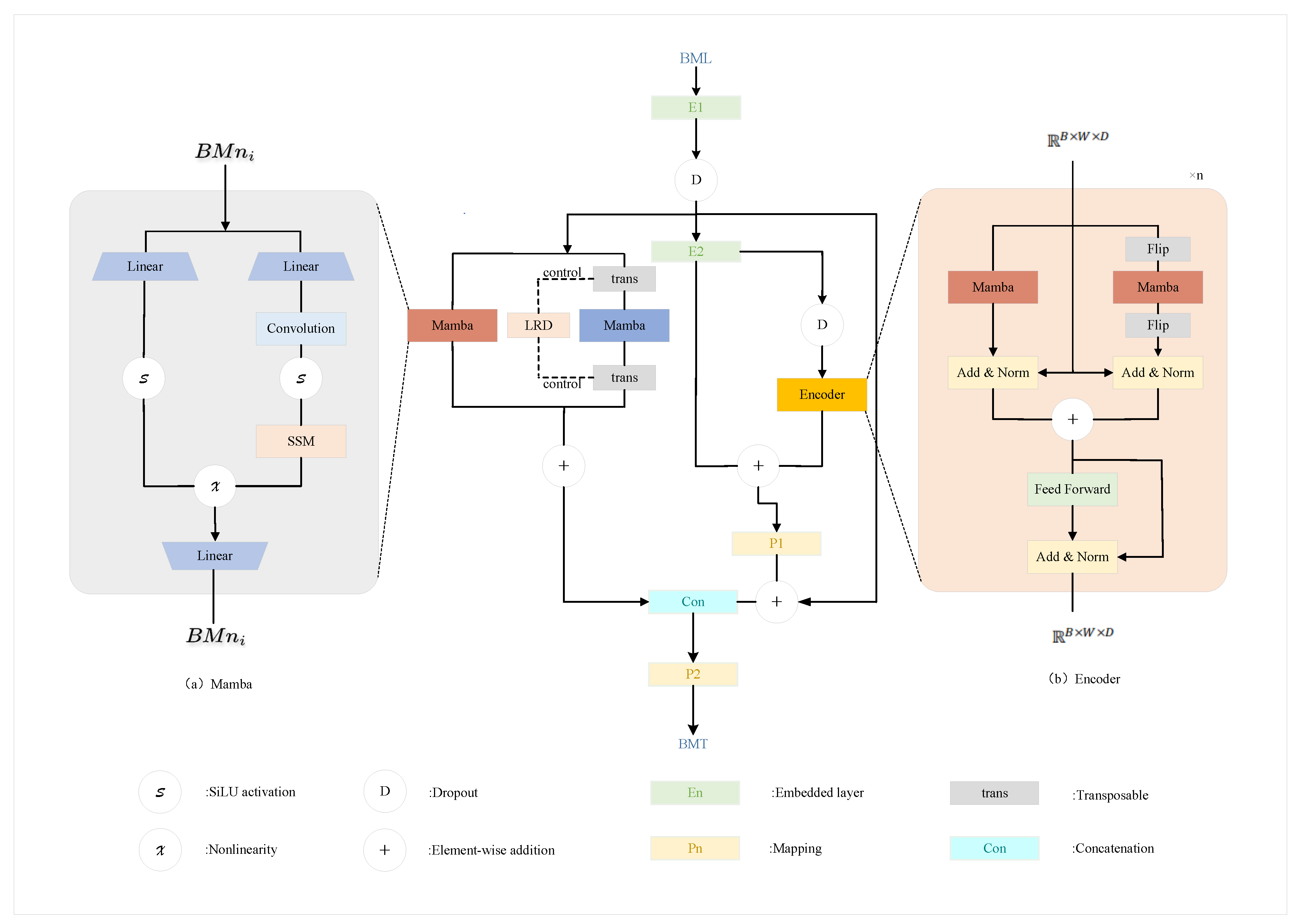
Figure 2.
Impact of hyperparameter settings on the ETTh1 dataset performance.
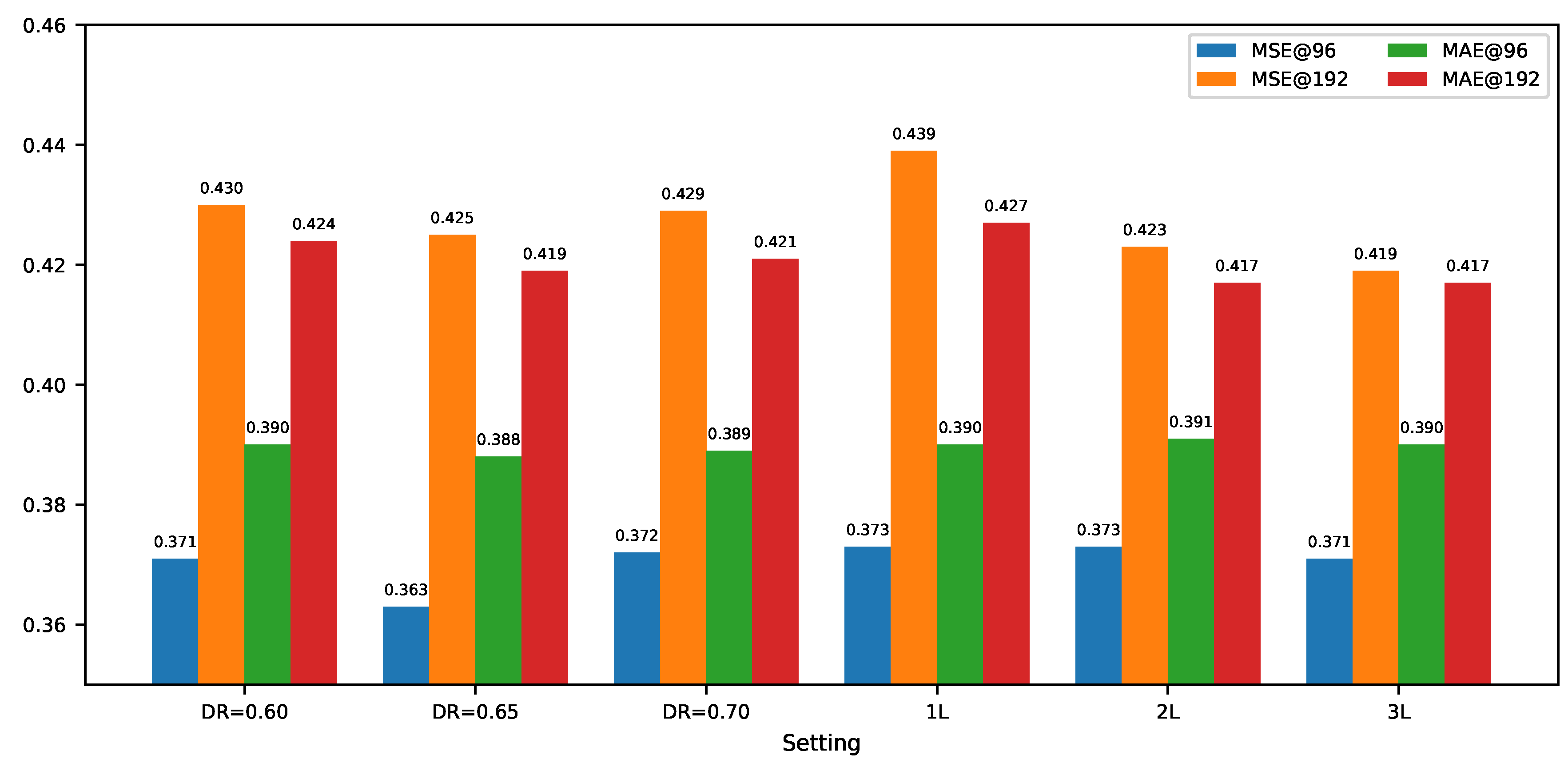
Table 1.
Dataset characteristics.
| Dataset | Variables | Granularity | Samples |
|---|---|---|---|
| ETTh1 | 7 | 1 hour | 17,420 |
| ETTh2 | 7 | 1 hour | 17,420 |
| ETTm1 | 7 | 15 min | 69,680 |
| ETTm2 | 7 | 15 min | 69,680 |
| Weather | 21 | 10 min | 52,696 |
| Electricity | 321 | 1 hour | 26,304 |
| Traffic | 862 | 1 hour | 17,544 |
Table 2.
Comparison of Forecasting Results Across Models
| Dataset | Metrics | Bi- Time SSM |
Bi- Mamba+ |
Time Machine |
i Trans former |
Patch TST |
Cross former |
Auto former |
D Linear |
Times Net |
Cross GNN |
|---|---|---|---|---|---|---|---|---|---|---|---|
| ETTh1 | MSE | 0.419 | 0.437 | 0.441 | 0.454 | 0.448 | 0.529 | 0.496 | 0.452 | 0.458 | 0.444 |
| MAE | 0.421 | 0.431 | 0.439 | 0.448 | 0.441 | 0.522 | 0.487 | 0.444 | 0.450 | 0.447 | |
| ETTh2 | MSE | 0.349 | 0.372 | 0.357 | 0.383 | 0.387 | 0.942 | 0.450 | 0.415 | 0.414 | 0.386 |
| MAE | 0.384 | 0.399 | 0.409 | 0.403 | 0.407 | 0.684 | 0.459 | 0.439 | 0.427 | 0.412 | |
| ETTm1 | MSE | 0.375 | 0.378 | 0.399 | 0.407 | 0.387 | 0.513 | 0.588 | 0.412 | 0.400 | 0.393 |
| MAE | 0.392 | 0.396 | 0.407 | 0.410 | 0.402 | 0.495 | 0.517 | 0.407 | 0.406 | 0.403 | |
| ETTm2 | MSE | 0.276 | 0.281 | 0.300 | 0.288 | 0.281 | 0.757 | 0.327 | 0.296 | 0.291 | 0.281 |
| MAE | 0.321 | 0.328 | 0.342 | 0.332 | 0.326 | 0.611 | 0.371 | 0.338 | 0.333 | 0.326 | |
| Weather | MSE | 0.244 | 0.243 | 0.252 | 0.252 | 0.262 | 0.259 | 0.338 | 0.273 | 0.259 | 0.266 |
| MAE | 0.272 | 0.272 | 0.284 | 0.285 | 0.283 | 0.315 | 0.382 | 0.291 | 0.287 | 0.294 | |
| Traffic | MSE | 0.429 | 0.404 | 0.426 | 0.428 | 0.481 | 0.550 | 0.617 | 0.622 | 0.620 | 0.657 |
| MAE | 0.282 | 0.272 | 0.308 | 0.282 | 0.305 | 0.304 | 0.372 | 0.371 | 0.336 | 0.396 | |
| Electricity | MSE | 0.175 | 0.166 | 0.186 | 0.178 | 0.196 | 0.244 | 0.227 | 0.221 | 0.193 | 0.235 |
| MAE | 0.259 | 0.263 | 0.272 | 0.270 | 0.281 | 0.334 | 0.338 | 0.305 | 0.295 | 0.321 |
Bold = best, Underline = second best.
Table 3.
Performance comparison with and without the encoder.
| Dataset | Full Model (Bi-TimeSSM) | Without Encoder | Relative Change | |||
| MSE | MAE | MSE | MAE | MSE | MAE | |
| ETTh1 | 0.419 | 0.421 | 0.420 | 0.422 | +0.2% | +0.2% |
| ETTh2 | 0.349 | 0.384 | 0.350 | 0.386 | +0.2% | +0.5% |
| ETTm1 | 0.375 | 0.392 | 0.376 | 0.394 | +0.2% | +0.5% |
| ETTm2 | 0.276 | 0.321 | 0.279 | 0.322 | +1.0% | +0.3% |
Table 4.
Performance comparison with and without parallel Mamba modules.
| Dataset | Full Model (Bi-TimeSSM) | Without Mamba | Relative Change | |||
| MSE | MAE | MSE | MAE | MSE | MAE | |
| ETTh1 | 0.419 | 0.421 | 0.432 | 0.427 | +3.1% | +1.4% |
| ETTh2 | 0.349 | 0.384 | 0.351 | 0.386 | +0.5% | +0.5% |
| ETTm1 | 0.375 | 0.392 | 0.405 | 0.401 | +8.0% | +2.2% |
| ETTm2 | 0.276 | 0.321 | 0.287 | 0.329 | +3.9% | +2.4% |
Disclaimer/Publisher’s Note: The statements, opinions and data contained in all publications are solely those of the individual author(s) and contributor(s) and not of MDPI and/or the editor(s). MDPI and/or the editor(s) disclaim responsibility for any injury to people or property resulting from any ideas, methods, instructions or products referred to in the content. |
© 2025 by the authors. Licensee MDPI, Basel, Switzerland. This article is an open access article distributed under the terms and conditions of the Creative Commons Attribution (CC BY) license (http://creativecommons.org/licenses/by/4.0/).
Copyright: This open access article is published under a Creative Commons CC BY 4.0 license, which permit the free download, distribution, and reuse, provided that the author and preprint are cited in any reuse.


