Submitted:
18 April 2025
Posted:
21 April 2025
You are already at the latest version
Abstract
Recently, deep learning has made significant strides in multivariate time series forecasting (MTSF). While frequency-domain-based methods have shown promising results, existing models often struggle with frequency misalignment when handling diverse frequency combinations, leading to reduced forecasting accuracy. To address these issues, we propose the Spectral Attention Module (SAM), which integrates temporal and frequency domain information to effectively capture both local and global dependencies in time series data. Within the frequency-domain module, we introduce an Extended Discrete Fourier Transform (EDFT) to overcome frequency misalignment challenges and design a Complex-Valued Spectral Attention Mechanism (CV-SAM) to identify and exploit complex relationships among different frequency combinations. To further capture inter-variable correlations, we propose the Bidirectional Variable Mamba (BV-Mamba). It uses linear layers to encode timestamps for each variable and employs the Mamba layer to extract inter-variable correlations, supported by a feedforward network to learn temporal dependencies. By combining the SAM and the BV-Mamba, we construct the SpectroMamba, which demonstrates superior performance over state-of-the-art methods in long-term time series forecasting across multiple real-world datasets.
Keywords:
time series analysis
; state space model
; complex-valued spectral attention
1. Introduction
In the real world, time series data exhibit diverse periodic patterns [1], manifesting not only across different segments of the same time series but also among various time series within the same dataset. While these periodic features are ubiquitous, their manifestations vary widely, reflecting the complexity and heterogeneity of time series data. Periodic time series often exhibit pronounced global dependencies, where data values at a given time are influenced by values at specific intervals in the past. In contrast, non-periodic time series predominantly display local dependencies [2], where data values at a given time are primarily determined by the values of nearby time points, lacking long-term consistency and predictability.
To gain a deeper understanding of the nature of time series data, time-domain and frequency-domain analyses have become two fundamental tools. Time-domain analysis focuses on the trends of data over time, making it particularly suitable for uncovering short-term fluctuations and instantaneous events. In contrast, frequency-domain analysis decomposes time series to identify their intrinsic periodic components [3], pro- viding strong support for understanding long-term trends and global correlations . By combining the strengths of time-domain and frequency-domain analyses, it becomes possible to comprehensively capture the multi-scale characteristics of time series data, which is crucial for addressing the complex challenges posed by real-world time series. Early research predominantly focused on time-domain analysis, as seen in methods like the Autoregressive Integrated Moving Average (ARIMA) [4] and Long Short- Term Memory (LSTM) [5] networks. In recent years, more advanced methods such as the Temporal Convolutional Network (TCN) [6] and Transformer-based architectures like the Time Series Transformer (TST) [7] have further improved the ability to capture temporal dependencies and model long-term relationships in time-series data. These approaches have laid a solid foundation for time-series forecasting, particularly in the time domain. With advancements in technology, increasing attention has shifted toward frequency-domain analysis, which has demonstrated immense potential, especially when integrated with deep learning techniques. For instance, the Frequency- domain Time-series Prediction (FITS) model [8] directly uses the frequency spectrum of time series as input, performs the prediction task in the frequency domain, and then restores the results to the time domain through a simple linear transformation. This approach not only improves prediction accuracy but also highlights the unique advantages of frequency-domain analysis. However, predicting directly in the frequency domain is not without challenges. One critical issue is efficiently extracting and integrating information about frequency combinations from the spectrum [9]. Harmonic sequences in the spectrum carry abundant information, but their complexity and diversity make this task highly challenging. Addressing these difficulties is key to unlocking the full potential of frequency-domain analysis in time-series forecasting. In addition to modeling temporal dependencies, another major challenge in multi- variate time series forecasting (MTSF) is capturing the correlations among variables [10]. Recent research has categorized MTSF models for modeling variable dependencies into two main types: variable-mixing models and variable-independent models [11]. Variable-mixing models extract features from all time series and project them into an embedding space to integrate information from multiple variables. In contrast, variable-independent models restrict their input to information from a single variable. Interestingly, recent studies have shown that variable-independent models outperform variable-mixing models on certain datasets [12]. However, this advantage comes at a cost: the omission of critical cross-variable information. This limitation can be detrimental, particularly when the variables are inherently correlated. Address- ing this trade-off is essential to improve the robustness and generalizability of MTSF models across diverse real-world scenarios.
To address the challenges outlined above, we developed a novel framework named SpectroMamba for modeling both cross-variable relationships and temporal dependencies. Specifically, we propose an innovative Spectral Attention Module (SAM), which integrates both time-domain and frequency-domain information, effectively capturing local and global dependencies within time series data. In the Spectral Attention Module, we introduce the Extended Discrete Fourier Transform (EDFT) to overcome frequency misalignment issues and design a Complex-Valued Spectral Attention Mechanism (CV-SAM) to identify and leverage the complex relationships between different frequency combinations. To model cross-variable relationships, we propose the Bidi rectional Variable Mamba (BV-Mamba) for variable-mixing methods, which is aimed at efficiently capturing and utilizing the intricate dependencies among multiple variables, thereby enhancing the performance of multivariate time series forecasting. In essence, the main contributions of our paper include:
- We introduce a novel Spectral Attention Module that integrates both time-domain and frequency-domain information to effectively capture local and global dependencies within time series data. It addresses frequency misalignment issues through the Extended Discrete Fourier Transform (EDFT) and utilizes a complex-valued spectral attention mechanism to identify and exploit intricate relationships among frequency combinations.
- We propose an innovative Bidirectional Variable Mamba that effectively captures and leverages complex relationships between multiple variables, enhancing the performance of multivariate time series forecasting.
- We present a comprehensive framework, called SpectroMamba that integrates the Spectral Attention and Variable Mamba modules. This unified approach is designed to tackle the challenges of multivariate time series forecasting and demonstrates superior performance on real-world datasets.
2. Related Works
2.1. Multivariate Time Series Forecasting
In multivariate time series forecasting (MTSF), model design typically falls into two main approaches: variable-independent modeling [9,12,13] and variable-dependent modeling [14,15,16]. In the variable-independent approach, each variable is processed independently, often using a shared underlying architecture. This approach is simpler and easier to implement. For example, PatchTST [12] introduced slicing and variable independence strategies to significantly improve the performance of the Transformer architecture. However, the variable-independent method tends to incur high compu- tational costs during both training and inference, leading researchers to explore more efficient modeling strategies. In contrast, the variable-dependent approach considers inter-channel dependencies when predicting future values, enabling more comprehen- sive capture of complex relationships within multivariate time series data. For instance, the RLinear [14] that the associations between channels comprehensively during fore- casting. The Crossformer [10] used serial time and variable attention mechanisms to capture dependencies across time and variables, while Dsformer [17] applied these two attention mechanisms in parallel, enhancing both efficiency and accuracy. Further- more, iTransformer [18] innovatively disruptED the traditional allocation of attention mechanisms and Feedforward networks in Transformers, focusing on capturing multi- variate correlations and learning nonlinear representations, demonstrating exceptional performance in multivariate time series forecasting tasks.
Frequency-domain prediction methods [9,19,20,21] have gained increasing attention due to their ability to reveal the periodic and frequency components within time series data, offering a unique perspective for capturing global dependencies. Recent advancements have focused on harnessing these frequency-domain features for improved forecasting. For example, Autoformer [19] utilized Fast Fourier Trans- form (FFT) to identify dominant periods and replaces the traditional self-attention mechanism with an autocorrelation mechanism, improving accuracy in long-sequence predictions. TimesNet [9] leveraged the top-k frequency amplitudes extracted via FFT, transforming one-dimensional time series into two-dimensional features to better capture spatial dependencies. FilM [20] used Legendre polynomials to project historical information and extracts frequency-domain features through FFT-based frequency enhancement layers. FreDo [21] introduced a simple yet efficient model, AverageTile, which uses Discrete Fourier Transform (DFT) to map time series into the frequency domain, enabling more accurate frequency feature extraction. These methods highlight the growing potential of frequency-domain approaches in improving time series fore- casting by capturing long-term dependencies and enhancing feature extraction across multiple scales.
Moreover, complex number processing is crucial for frequency-domain analysis, as real-valued representations may fail to capture deeper features within the frequency domain. For instance, StemGNN [22] integrated Graph Fourier Transform (GFT) to model inter-sequence dependencies and uses DFT to capture temporal dependencies. However, its separation of real and imaginary parts of complex numbers may limit its ability to fully capture the complex interactions in the data. To address this, many methods optimize frequency-domain feature extraction using complex- valued neural networks. For example, FEDformer [15] introduced learnable complex weights for frequency-domain transformations and offers two versions based on DFT and Discrete Wavelet Transform (DWT), enabling better exploration of frequency- domain relationships. FITS [8] applied FFT to transform time series into the frequency domain, followed by complex-valued linear layers and low-pass filters to attenuate high- frequency noise. FreTS [2] designed a real-valued MLP structure that mimics complex number operations, allowing for accurate handling of both real and imaginary parts of frequency coefficients.
2.2. State Space Model
Sequence modeling has been a crucial aspect of various applications, including natural language processing, computer vision, and video understanding. Traditional sequence- to-sequence models with soft attention have shown success in these domains but suffer from quadratic time and space complexity during decoding, limiting their real-time applicability. To address this issue, Chiu et al. [23] introduced Monotonic Chunkwise Attention (MoChA), a linear-time attention mechanism that performs soft attention over adaptively-located chunks of the input sequence. While models like the Structured State-Spaces for Long-Form Video Understanding (S4) have been effective, treating all image-tokens equally can impact efficiency and accuracy. Wang et al. [24] pro- posed a Selective S4 (S5) model that uses a lightweight mask generator to selectively choose informative image tokens, resulting in more efficient and accurate modeling of long-term spatiotemporal dependencies in videos. Gu et al. [25] identified the computational inefficiency of Transformers on long sequences and introduced Mamba, a linear-time sequence modeling approach with selective state spaces. The Mamba layer offers an efficient selective state space model that is effective in various domains, including NLP and computer vision. Additionally, incorporating Mamba in Multiple Instance Learning (MIL) for long sequence modeling has shown promise, especially with the Sequence Reordering Mamba (SR-Mamba) [26] that considers the order and distribution of instances. State space models like Mamba have also been explored in motion generation tasks, showcasing improvements in FID scores and speed compared to previous methods. Qiao et al. [27] proposed VL-Mamba, a multimodal large language model based on state space models, to address the computational overhead of attention mechanisms in Transformers. In the realm of computer vision, lu et al. [28] tackled the challenge of designing an appropriate scanning method for 4D light fields by employing state space models on informative 2D slices to enhance spatial contextual information and structure information.
3. Preliminary
3.1. Problem Definition
Long-term time series forecasting can be viewed as a sequence-to-sequence problem. Given a multivariate time series, where L is the size of the lookback window and N is the number of variables, the goal is to forecast the next T time steps.
Formally, let the historical time series data for the past L time steps, each containing information from N variables, be represented as:
X = {xt−L, xt−L+1, ..., xt−1} where xt ∈ RN
The objective is to predict the future T steps:
where X represents the historical data and Y represents the future predictions. The goal of the model is to infer Y from X, i.e., to predict future values based on past data.
Y = {yt, yt+1, ..., yt+T −1}
3.2. Discrete Fourier Transform
The Discrete Fourier Transform (DFT) [29,30] is a mathematical transformation that converts a time series into its frequency domain representation, revealing the frequency components of the data. Specifically, for an input sequence of length L, the DFT spectrum is computed as follows:
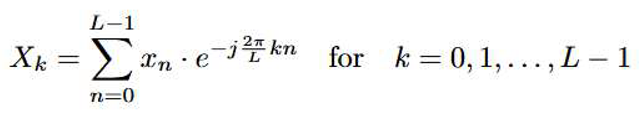 where xn is the input sequence of length L, Xk is the complex frequency domain representation, k represents the index of the frequency component, j is the imaginary unit, e−j2πkn is the complex exponential function that captures the oscillatory nature of the frequency components.
The Inverse Discrete Fourier Transform (IDFT) is the reverse operation of the DFT. It converts the frequency-domain signal obtained by the DFT back into the original time-domain signal. The IDFT is computed as follows:
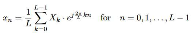 where Xk is the frequency-domain representation of the signal, xn is the time-domain signal after applying the inverse transform, j is the imaginary unit, L is the length of the sequence.
3.3. State Space Models
State Space Models (SSMs) [31] are widely used for modeling cyclic processes with hidden states. They describe the evolution of system states using first-order differential equations and relate the hidden states to the output sequence through a second set of equations. The general form of the system is given by:
h (t) = Ah(t) + Bx(t),
y(t) =e Ch(t) + Dx(t),
Here, A represents the state matrix that governs how the current state influences its rate of change, B is the input matrix, and C and D are the output and feed-through matrices, respectively.
In practical applications, this continuous system is discretized for computational efficiency, typically under the zero-order hold assumption [32]. The discretized version of the system is obtained by converting the continuous matrices A and B to their discrete counterparts over a time step:
Thus, the discretized state space model can be written as:
A key limitation of this approach is that the model parameters remain fixed regard- less of the input sequence. To address this issue, the Mamba framework introduces a selective state-space model, where the parameters adapt according to the input data, enabling more effective selective information processing across different time sequences [33]. This adaptation is expressed by the following equations:

Here, fB(xt), fC(xt), and fA(xt) are linear functions that adapt the model’s parameters based on the input sequence, allowing for a more dynamic and responsive system.
4. Proposed Method
4.1. Overall Framework
Our proposed SpectroMamba architecture is shown in Figure 1. Given the input time series , we first apply Reverse Instance Normalization(RevIN) [34] to process the input, a method originally designed to address distributional shifts in the time domain. Next, we apply the extended Discrete Fourier Transform (DFT) to transform the data into the frequency domain, enabling the capture of global correlations in the time series. Subsequently, we use the Inverse Discrete
Fourier Transform (IDFT) to map the frequency-domain data back to the time domain. On this basis, we use a Feed Forward Network (FFN) to capture local dependencies within the time domain. Furthermore, we introduce the Mamba layer to extract correlations among different variables, and combine it with the FFN to further learn temporal dependencies. The overall architecture can be formalized by the following equations:
4.2. Spectral Attention Module
The SAM is built upon the Transformer encoder architecture and is specifically designed to process complex-valued data in the frequency domain. All computa- tions within the module are conducted in the complex domain, ensuring the spectral characteristics of the input data are fully preserved.
The SAM takes as input the univariate spectrum , generated using the Extended DiscreteFourier Transform (DFT), where represents the length of the spectrum. This design leverages the properties of complex-valued representations to model and capture intricate dependencies in the frequency domain effectively, as shown in Figure 1.
The traditional multi-head attention mechanism of Transformers is designed for real-valued data, making it challenging to directly apply to complex-valued data in the spectral domain. To address this limitation, we propose a Complex-Valued Spectra Attention Mechanism, which treats the real and imaginary components of complex- valued data separately as inputs, enabling effective modeling in the complex domain through real-valued operations, as shown in Figure 1.
Complex-Valued Spectra Attention Mechanism. This CV-SAM leverages a fundamental property of complex-valued functions: for any complex-valued function f : Cn→ C and any complex vector x = a + ib, the function can be expressed as:
where u(a, b) and v(a, b) are real-valued functions representing the real and imaginary parts of the complex function, respectively.
f (x) = f (a + ib) = u(a, b) + iv(a, b),
Using this property, the attention mechanism decomposes the complex-valued inputs into their real and imaginary parts, applies real-valued transformations independently, and then recombines the results into a single complex-valued output. This approach preserves the integrity of the complex domain while maintaining compatibility with the underlying operations of the Transformer architecture. First, we represent the input spectrum as a complex tensor, where is the time step and is the feature dimension. Decompose the complex input into real and imaginary parts:
X = Xreal + iXimag, Xreal, Ximag ∈ RL×d
Then, Generate complex query (Q), key (K), value (V) through real projection matrix WQ, WK, WV ∈ Cd×d:
where WQ, WK, WV are a real-valued projection matrix, and Q, K, V are all complex- valued matrices. The attention mechanism is calculated in the complex domain using the following formula:
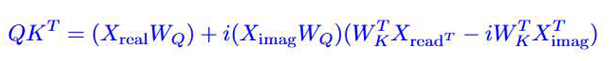
Q = X · WQ = (XrealWQ) + i(XimagWQ),
K = X · WK = (XrealWK) + i(XimagWK),
V = X · WV = (XrealWV ) + i(XimagWV ).
Further decomposition into real and imaginary parts:
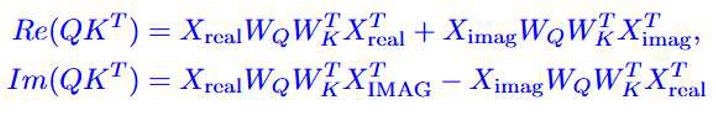
From the perspective of signal processing, this decomposition has clear physical meaning. The real part calculation captures the similarity between amplitude features and effectively reflects the degree of energy alignment of frequency components; while the imaginary part calculation focuses on capturing the interaction of phase differ- ences and shows high sensitivity to frequency offset and phase modulation. Through this design, CV-SAM can simultaneously process amplitude and phase information in spectral data, overcoming the inherent limitations of traditional real-domain attention mechanisms in spectral analysis.
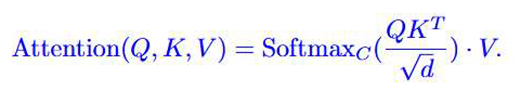
To solve the problem of probability normalization in the complex domain, we propose a solution to treat the real and imaginary parts independently. For complex attention scores A = Areal + iAimag, we apply the Softmax function to the real and imaginary parts separately:
SoftmaxC(A) = Softmax(Areal) + iSoftmax(Aimag).
The theoretical basis of this normalization strategy is
that the complex probability distribution theoretically needs to satisfy the
condition of  =
1, but directly normalizing the complex amplitude will inevitably lead to the
loss of phase information. By independently normalizing the real and imaginary
parts, we ensure the validity of the probability distribution in the real
subspace while retaining the statis- tical characteristics of the phase
difference, so that the model can better utilize the rich information provided
by the spectral phase.
=
1, but directly normalizing the complex amplitude will inevitably lead to the
loss of phase information. By independently normalizing the real and imaginary
parts, we ensure the validity of the probability distribution in the real
subspace while retaining the statis- tical characteristics of the phase
difference, so that the model can better utilize the rich information provided
by the spectral phase.Finally, the complex attention output is calculated as follows:
Expand to calculate the real and imaginary parts:
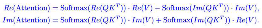
This calculation method combines the interaction between the real and imaginary parts. The real output enhances the signal strength by promoting the feature representation of consistent amplitude, while the imaginary output enhances the model’s perception of frequency modulation and phase changes by capturing the dynamic changes of the phase. The synergy of this dual mechanism gives CV-SAM a significant advantage in processing complex spectral data.
4.3. Bidirectional Variable Mamba
While the global attention mechanism in the Transformer architecture captures inter- actions among all variables, its computational complexity increases exponentially with the number of variables, limiting its applicability in large-scale scenarios. In contrast, the Mamba module efficiently evaluates variable importance through a selection mechanism, with computational overhead increasing linearly with the number of variables. However, due to the unidirectional nature of the selection mechanism, the Mamba module can only establish relationships based on preceding variables, making it challenging to fully capture global variable dependencies. Consequently, the standalone Mamba module exhibits limitations in handling complex multivariable scenarios: : (1) It can only capture the dependencies between variables based on a single direction of the input sequence (e.g., from left to right). (2) This unidirectionality may lead to missing global dependencies between variables, especially in complex multivariate scenarios.
To overcome the aforementioned limitations, we propose a Bidirectional Variable Mamba by combining two Mamba modules, enabling global interaction modeling among variables, as shown in Figure 1. Specifically, one Mamba module is designed to capture forward dependencies among variables, while the other focuses on backward dependencies. This bidirectional design effectively addresses the shortcomings of unidirectional mechanisms, allowing the module to comprehensively account for mutual relationships among all variables. By weightedly combining the outputs of the forward and reverse modules, the global interactions between modeling variables are comprehensively modeled. The core of this design is to capture the interrelationships between variables, rather than simply treating them as ”past” or ”future” dependencies in the time series.
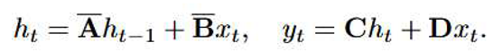
The core of the Mamba module is the state space model (SSM) based on the selection mechanism. Its basic calculation formula is as follows. State update formula: For the input sequence, the state update of the Mamba module can be expressed as:
ht = Aht−1 + Bxt.
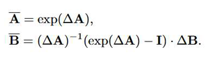
The output yt of the module is obtained by mapping the hidden state ht through the output matrix. In order to apply the continuous state space model on the discrete time series, the parameters and need to be converted through the discretization formula:
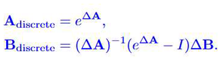 where ∆ is the time step, I is the identity matrix.
In the Mamba module, the selection mechanism enables selective modeling of vari- able dependencies by allowing parameters A, B, and C to be dynamically adjusted depending on the input xt. This input dependency enables the model to dynamically filter irrelevant information and remember relevant information.
Here is how the bidirectional modeling can be expressed mathematically: For the forward Mamba module, capturing forward dependencies:
Hforward = Mamba(Hinput)
For the backward Mamba module, capturing backward dependencies:
where denotes the reversed input sequence to capture backward relationships.
The final output of the Bidirectional Mamba layer combines both directions as follows:
where α and β are learnable weights to adaptively balance the contributions of for- ward and backward dependencies during training. This design ensures comprehensive modeling of all variable interactions.
Houtput = αHforward + βHbackward
5. Experiments
To evaluate the effectiveness of our proposed DWSL prediction framework, we con- ducted extensive experiments on eight publicly available datasets. These datasets cover real-world multivariate data, including five power energy datasets and one meteorological dataset. Detailed statistics for each dataset can be found in Table 1. Among these datasets, the Solar-Energy and Electricity datasets are particularly significant due to their inclusion of more variables, allowing for a more comprehensive assessment of the performance of our method. The datasets are described as follows:
- ETT Dataset [7]: It originates from two power substations and spans from July 2016 to July 2018, recording seven variables, including load and oil temperature. The ETTm1 and ETTm2 datasets are recorded every 15 minutes, with a total of 69,680 time steps. The ETTh1 and ETTh2 datasets are hourly equivalents of ETTm1 and ETTm2, each containing 17,420 time steps.
- Electricity Dataset [19]: It contains hourly power consumption data from 321 users, covering a two-year period, with a total of 26,304 time steps.
- Solar-Energy Dataset [35]: It records solar energy generation from 137 photo- voltaic stations in Alabama in 2006, with samples taken every 10 minutes.
- Weather Dataset [19]: Collected by the Max Planck Institute for Biogeochem- istry’s weather stations in 2020, this dataset includes 21 meteorological factors, such as atmospheric pressure, temperature, and humidity, with data recorded every 10 minutes.
- Traffic Dataset [19]: Covering the period from July 2016 to July 2018, this dataset records road occupancy data from 862 sensors deployed on highways in the San Francisco Bay Area. The data is collected every hour, providing detailed temporal resolution to analyze traffic patterns and dynamics over the two-year period.
- Through experiments on these diverse real-world datasets, we demonstrate the per- formance of the SpectroMamba framework, validating its versatility and applicability across various scenarios.
5.1. Experimental Settings
In this study, based on previous research [7], we processed the datasets with a step size of 1 to construct diverse input-output pairs, aiming to enhance the model’s learning efficiency and generalization capability. To ensure consistency and stability during the model training process, we applied zero-mean normalization preprocessing to the training, validation, and test sets using the mean and standard deviation of the training set. This standardization accelerates the model’s convergence rate and improves its performance.
For model configuration, we set the input sequence length I to 96. We systematically explored various combinations of hyperparameters, including learning rates from 10−4 to 0.05, encoder layers from 1 to 3, and model dimensions dmodel ranging from 128 to 512, in an effort to find the optimal configuration that maximizes model performance.
Regarding evaluation metrics, we selected Mean Squared Error (MSE) as the loss function. To comprehensively assess the model’s performance, follow [36], we also used both MSE and Mean Absolute Error (MAE), which reflect the model’s predictive accuracy from different perspectives.
The Adam optimizer was chosen to train our model due to its efficiency in handling large-scale machine learning tasks. Additionally, we incorporated an early stopping strategy to effectively prevent overfitting and ensure the model’s generalization ability on new data. All experiments were conducted on high-performance computing nodes equipped with an NVIDIA RTX 4090 GPU with 24GB of VRAM, and the software environment was developed and deployed using the PyTorch framework.
5.2. Compared to Sota Methods
To comprehensively evaluate the effectiveness of the proposed algorithm, this study carefully selects a range of advanced models as comparison benchmarks. These models not only represent different strategies for handling variable interactions and independencies, but also reflect the latest developments in deep learning architectures for time series analysis. In particular, given the exceptional ability of the Transformer architecture to capture long-range dependencies and model complex temporal patterns, we prioritize it as one of the main focuses of our study. On this basis, we chose six representative Transformer-based models, including Autoformer [19], FEDformer [15], Stationary [37], Crossformer [10], and iTransformer [18]. Additionally, considering the growing attention and strong performance of Multi-Layer Perceptron (MLP) models in recent years due to their simplicity and effectiveness, we also included TiDE [38], a prominent and influential MLP variant, in our study. To further enrich the comparison framework, we introduce three CNN models—SCINet [39], TimesNet [9], and another RNN model-DeepAR [40] and GRU [41]. These CNN-based models, with their unique advantages in efficiently extracting multivariate time series features, provide crucial supplementary perspectives for our research.
As shown in Table 2, SpectroMamba demonstrates a significant advantage in both MAE and MSE metrics, thoroughly validating its exceptional performance and generalization capability. In experiments conducted across various public datasets and different prediction time points, SpectroMamba consistently outperforms most com- parison models in terms of Mean Squared Error (MSE) and Mean Absolute Error (MAE). This is particularly evident in long-term sequence prediction tasks, where its accuracy advantage is most pronounced, highlighting its superior ability to capture complex long-term temporal dependencies.
To enhance clarity, we visualized the prediction performance of SpectroMamba on the ETTm1 dataset for forecast horizons of 96, 192, 336, and 720 steps. Figure 2, Figure 3, Figure 4, and Figure 5 illustrate the corresponding prediction curves, vividly demonstrating the model’s remarkable capability to capture both short-term and long-term dependencies with precision.
Compared to advanced Transformer-based models such as iTransformer and Cross- former, SpectroMamba exhibits lower prediction errors. This is attributed to its effective extraction of multi-scale features through the spectral decomposition module, coupled with a dynamic self-attention mechanism that enhances the modeling of inter- actions between the time and variable dimensions. Additionally, when compared to methods like TimesNet and TiDE, SpectroMamba demonstrates stronger adaptability in handling different types of time series data. Whether dealing with the highly peri- odic solar energy data or the non-periodic electricity load data, its prediction results remain consistently stable and efficient.
Furthermore, SpectroMamba excels not only in single-domain tasks, such as weather data prediction, but also in cross-domain tasks, such as distributed photovoltaic power forecasting, showcasing its robustness and generalization ability. Its well-designed parameters and moderate model size help to improve prediction accuracy while effectively avoiding overfitting, resulting in high training efficiency.
Overall, by integrating multi-scale feature extraction and dynamic variable dependency modeling, SpectroMamba excels not only in capturing global features but also in uncovering fine-grained dependencies within the data, making it a powerful tool for a wide range of time series forecasting tasks.
6. Ablation Study
Individual Component
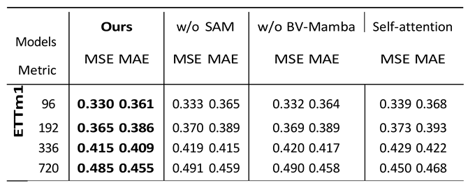
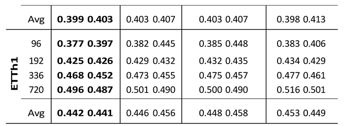
To validate the effectiveness of the Spectral Attention Module and the Bidirectional Variable Mamba in the SpectroMamba model, we conducted detailed ablation experiments on the ETTh1 and ETTm1 datasets, analyzing the specific contribution of these two components to the model’s performance. The experimental design included two sets of comparative models: 1) Removing the Spectral Attention Module from the SpectroMamba framework, labeled as ”w/o SAM”; 2) Removing the Bidirectional Variable Mamba, labeled as ”w/o BV-Mamba.” 3) Replace SAM with traditional self-attention mechanism, labeled as ”self-attention”.
To ensure fairness and the comparability of results, all models were tested under the same dataset, experimental conditions, and hyperparameter settings, including the same learning rate, batch size, and number of iterations.
The ablation study presented in Table 3 provides a detailed analysis of the individual contributions of the spectral attention module (SAM) and the bidirectional variable Mamba (BV-Mamba) to the overall performance of the SpectroMamba model. The results clearly indicate that the full model, which incorporates both SAM and BV- Mamba, consistently outperforms the ablated versions across various datasets (ETTm1 and ETTh1) and different prediction horizons (96, 192, 336, and 720 time steps). In particular, when the SAM module is removed, the model shows a slight increase in MSE and MAE, indicating that SAM plays a critical role in effectively capturing multi- scale spectral features and enhancing the model’s ability to learn complex temporal dependencies. Similarly, when the BV-Mamba module is omitted, the performance degradation is also noticeable, particularly for longer forecasting horizons, suggesting that BV-Mamba is vital for capturing the interdependencies between variables over extended time periods.
As shown in Table 3, the spectral attention module consistently demonstrated significant advantages across all prediction horizons, particularly in handling datasets with complex spectral features. For instance, in the 720-step prediction task on the ETTm1 dataset, the model equipped with the spectral attention module achieved MSE and MAE values of 0.485 and 0.455, respectively, compared to 0.450 and 0.468 for the traditional self-attention mechanism. This represents improvements of 7.2% and 2.8% in MSE and MAE, respectively.
These experimental results highlight the superior ability of the spectral attention module to capture spectral features and complex temporal dependencies in the data, compared to the traditional self-attention mechanism. Particularly for long-term prediction tasks, the spectral attention module excels at extracting and leveraging multi-scale features, significantly enhancing the model’s predictive accuracy and robustness.
To systematically evaluate the performance stability of the proposed model when confronted with noise in the input data, we conducted experiments on the ETTm2 dataset. In these experiments, Gaussian noise was introduced to a selected subset of the input data to simulate real-world uncertainties and disturbances. Specifically, for any given time series input X(t−T +1:t) , Gaussian perturbations were applied, as mathematically expressed below:
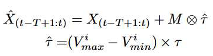 where M represents a randomly generated binary mask used to adjust the noise injection ratio, this ratio was set at 10%, 20%, 30%, 40%, and 50% to comprehensively evaluate the model’s performance under different noise levels. and refer to the maximum and minimum values of the i-th feature dimension, respectively, while τ ~Gauss(0, 1) is a random sample drawn from a standard normal distribution, serving as the noise source.
Figure 6 presents a comparison of the MAE for the SpectroMamba, iTransformer, and TimesNet models on the ETTm2 dataset under different noise levels. As the noise intensity increased, SpectroMamba exhibited a slower MAE growth trend compared to iTransformer and TimesNet. This result not only confirms the superior robustness of SpectroMamba in handling noisy data but also provides strong theoretical support for its ability to manage abnormal data fluctuations in practical applications.
7. Conclusion
In this paper, we presented SpectroMamba, a novel framework for multivariate time series forecasting (MTSF) that effectively models both temporal dependencies and cross-variable relationships. Our proposed Spectral Attention Module (SAM) inte- grates both time-domain and frequency-domain information, capturing local and global dependencies in time series data. The module incorporates the Extended Discrete Fourier Transform (EDFT) to address frequency misalignment issues and employs a Complex-Valued Spectral Attention Mechanism (CV-SAM) to identify and utilize intricate relationships among frequency combinations. Complementing SAM, the Bidirectional Variable Mamba (BV-Mamba) efficiently captures cross-variable relationships, overcoming the trade-offs between variable-mixing and variable-independent methods. Through comprehensive experiments on multiple real-world datasets, SpectroMamba consistently outperformed state-of-the-art models in both short-term and long-term forecasting tasks. These results demonstrate its ability to extract meaningful dependencies from complex multivariate data, significantly enhancing predictive accuracy.
References
- Zhuang, W., Fan, J., Fang, J., Fang, W., Xia, M.: Rethinking general time series analysis from a frequency domain perspective. Knowledge-Based Systems 301, 112281 (2024). [CrossRef]
- Yi, K., Zhang, Q., Fan, W., Wang, S., Wang, P., He, H., An, N., Lian, D., Cao, L., Niu, Z.: Frequency-domain mlps are more effective learners in time series forecasting. Advances in Neural Information Processing Systems 36 (2024).
- Luo, Y., Lyu, Z., Huang, X.: Tfdnet: Time-frequency enhanced decomposed network for long-term time series forecasting. arXiv preprint arXiv:2308.13386 (2023). [CrossRef]
- Box, G.E., Jenkins, G.M., Reinsel, G.C., Ljung, G.M.: Time Series Analysis: Forecasting and Control. John Wiley & Sons, (2015).
- Hochreiter, S.: Long short-term memory. Neural Computation MIT-Press (1997).
- Bai, S., Kolter, J.Z., Koltun, V.: An empirical evaluation of generic convolutional and recurrent networks for sequence modeling. arXiv preprint arXiv:1803.01271 (2018).
- Zhou, H., Zhang, S., Peng, J., Zhang, S., Li, J., Xiong, H., Zhang, W.: Informer: Beyond efficient transformer for long sequence time-series forecasting. In: Proceedings of the AAAI Conference on Artificial Intelligence, vol. 35, pp. 11106–11115 (2021). [CrossRef]
- Xu, Z., Zeng, A., Xu, Q.: Fits: Modeling time series with 10k parameters. arXiv preprint arXiv:2307.03756 (2023).
- Wu, H., Hu, T., Liu, Y., Zhou, H., Wang, J., Long, M.: Timesnet: Tem- poral 2d-variation modeling for general time series analysis. arXiv preprint arXiv:2210.02186 (2022).
- Zhang, Y., Yan, J.: Crossformer: Transformer utilizing cross-dimension depen- dency for multivariate time series forecasting. In: The Eleventh International Conference on Learning Representations (2023).
- Qi, S., Wen, L., Li, Y., Yang, Y., Li, Z., Rao, Z., Pan, L., Xu, Z.: Enhancing multivariate time series forecasting with mutual information-driven cross-variable and temporal modeling. arXiv preprint arXiv:2403.00869 (2024).
- Nie, Y., Nguyen, N.H., Sinthong, P., Kalagnanam, J.: A time series is worth 64 words: Long-term forecasting with transformers. arXiv preprint arXiv:2211.14730 (2022).
- Zhou, X., Wang, W., Buntine, W., Qu, S., Sriramulu, A., Tan, W., Bergmeir, C.: Scalable transformer for high dimensional multivariate time series forecasting. In: Proceedings of the 33rd ACM International Conference on Information and Knowledge Management, pp. 3515–3526 (2024).
- Zeng, A., Chen, M., Zhang, L., Xu, Q.: Are transformers effective for time series forecasting? In: Proceedings of the AAAI Conference on Artificial Intelligence, vol. 37, pp. 11121–11128 (2023).
- Zhou, T., Ma, Z., Wen, Q., Wang, X., Sun, L., Jin, R.: Fedformer: Fre- quency enhanced decomposed transformer for long-term series forecasting. In: International Conference on Machine Learning, pp. 27268–27286 (2022). PMLR.
- Yu, G., Zou, J., Hu, X., Aviles-Rivero, A.I., Qin, J., Wang, S.: Revitalizing multi- variate time series forecasting: Learnable decomposition with inter-series depen- dencies and intra-series variations modeling. arXiv preprint arXiv:2402.12694 (2024).
- Yu, C., Wang, F., Shao, Z., Sun, T., Wu, L., Xu, Y.: Dsformer: A double sampling transformer for multivariate time series long-term prediction. In: Proceedings of the 32nd ACM International Conference on Information and Knowledge Management, pp. 3062–3072 (2023).
- Liu, Y., Hu, T., Zhang, H., Wu, H., Wang, S., Ma, L., Long, M.: itransformer: Inverted transformers are effective for time series forecasting. arXiv preprint arXiv:2310.06625 (2023).
- Wu, H., Xu, J., Wang, J., Long, M.: Autoformer: Decomposition transform- ers with auto-correlation for long-term series forecasting. Advances in neural information processing systems 34, 22419–22430 (2021).
- Zhou, T., Ma, Z., Wen, Q., Sun, L., Yao, T., Yin, W., Jin, R., et al.: Film: Frequency improved legendre memory model for long-term time series forecasting. Advances in neural information processing systems 35, 12677–12690 (2022).
- Sun, F.-K., Boning, D.S.: Fredo: frequency domain-based long-term time series forecasting. arXiv preprint arXiv:2205.12301 (2022).
- Cao, D., Wang, Y., Duan, J., Zhang, C., Zhu, X., Huang, C., Tong, Y., Xu, B., Bai, J., Tong, J., et al.: Spectral temporal graph neural network for multivariate time-series forecasting. Advances in neural information processing systems 33, 17766–17778 (2020).
- Chiu, C.-C., Raffel, C.: Monotonic chunkwise attention. arXiv preprint arXiv:1712.05382 (2017).
- Wang, J., Zhu, W., Wang, P., Yu, X., Liu, L., Omar, M., Hamid, R.: Selective structured state-spaces for long-form video understanding. In: Proceedings of the IEEE/CVF Conference on Computer Vision and Pattern Recognition, pp. 6387– 6397 (2023).
- Ali, A., Zimerman, I., Wolf, L.: The hidden attention of mamba models. arXiv preprint arXiv:2403.01590 (2024).
- Yang, S., Wang, Y., Chen, H.: Mambamil: Enhancing long sequence modeling with sequence reordering in computational pathology. In: International Conference on Medical Image Computing and Computer-Assisted Intervention, pp. 296–306 (2024). Springer.
- Qiao, Y., Yu, Z., Guo, L., Chen, S., Zhao, Z., Sun, M., Wu, Q., Liu, J.: Vl-mamba: Exploring state space models for multimodal learning. arXiv preprint arXiv:2403.13600 (2024).
- Lu, Y., Wang, S., Wang, Z., Xia, P., Zhou, T., et al.: Lfmamba: Light field image super-resolution with state space model. arXiv preprint arXiv:2406.12463 (2024).
- Burke, K., Wagner, L.O.: Dft in a nutshell. International Journal of Quantum Chemistry 113(2), 96–101 (2013).
- Oppenheim, A.V., Verghese, G.C.: Signals, Systems & Inference. Pearson London, (2017).
- Gu, A., Dao, T.: Mamba: Linear-time sequence modeling with selective state spaces. arXiv preprint arXiv:2312.00752 (2023).
- Gu, A., Johnson, I., Goel, K., Saab, K., Dao, T., Rudra, A., R´e, C.: Combin- ing recurrent, convolutional, and continuous-time models with linear state space layers. Advances in neural information processing systems 34, 572–585 (2021).
- Gu, A., Dao, T., Ermon, S., Rudra, A., R´e, C.: Hippo: Recurrent memory with optimal polynomial projections. Advances in neural information processing systems 33, 1474–1487 (2020).
- Kim, T., Kim, J., Tae, Y., Park, C., Choi, J.-H., Choo, J.: Reversible instance normalization for accurate time-series forecasting against distribution shift. In: International Conference on Learning Representations (2021).
- Lai, G., Chang, W.-C., Yang, Y., Liu, H.: Modeling long-and short-term tempo- ral patterns with deep neural networks. In: The 41st International ACM SIGIR Conference on Research & Development in Information Retrieval, pp. 95–104 (2018).
- Chicco, D., Warrens, M.J., Jurman, G.: The coefficient of determination r-squared is more informative than smape, mae, mape, mse and rmse in regression analysis evaluation. Peerj computer science 7, 623 (2021).
- Liu, Y., Wu, H., Wang, J., Long, M.: Non-stationary transformers: Exploring the stationarity in time series forecasting. Advances in Neural Information Processing Systems 35, 9881–9893 (2022).
- Das, A., Kong, W., Leach, A., Mathur, S., Sen, R., Yu, R.: Long-term forecasting with tide: Time-series dense encoder. arXiv preprint arXiv:2304.08424 (2023).
- Liu, M., Zeng, A., Chen, M., Xu, Z., Lai, Q., Ma, L., Xu, Q.: Scinet: Time series modeling and forecasting with sample convolution and interaction. Advances in Neural Information Processing Systems 35, 5816–5828 (2022).
- Salinas, D., Flunkert, V., Gasthaus, J., Januschowski, T.: Deepar: Probabilis- tic forecasting with autoregressive recurrent networks. International journal of forecasting 36(3), 1181–1191 (2020).
- Cho, K., Van Merri¨enboer, B., Gulcehre, C., Bahdanau, D., Bougares, F., Schwenk, H., Bengio, Y.: Learning phrase representations using rnn encoder- decoder for statistical machine translation. arXiv preprint arXiv:1406.1078 (2014).
Figure 1.
The framework overview of our proposed SpectroMamba.
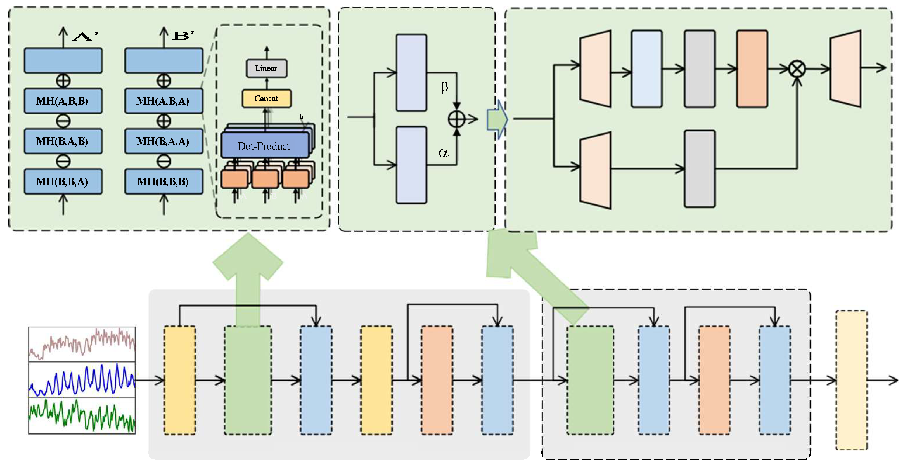
Figure 2.
Visualization of input-96-predict-96 results on the ETTm1 dataset.
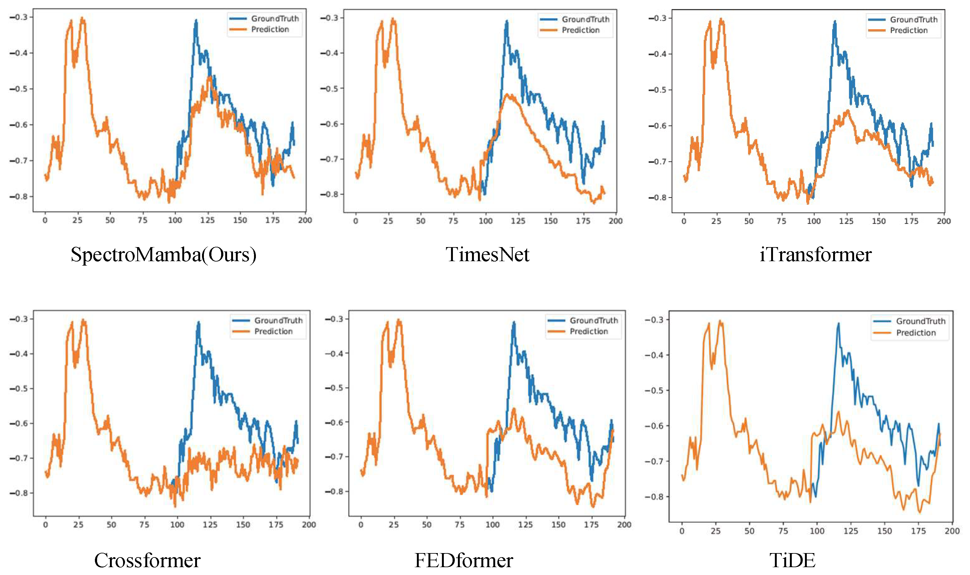
Figure 3.
Visualization of input-96-predict-192 results on the ETTm1 dataset.
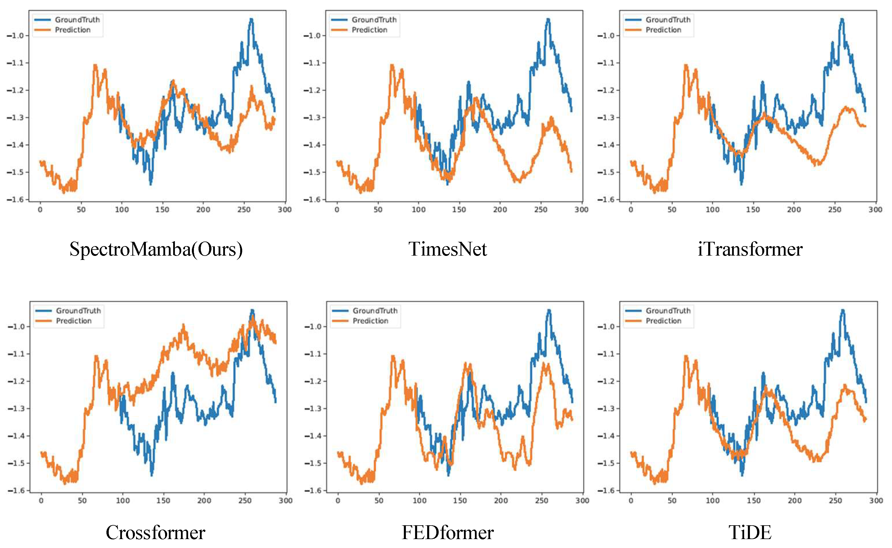
Figure 4.
Visualization of input-96-predict-336 results on the ETTm1 dataset.
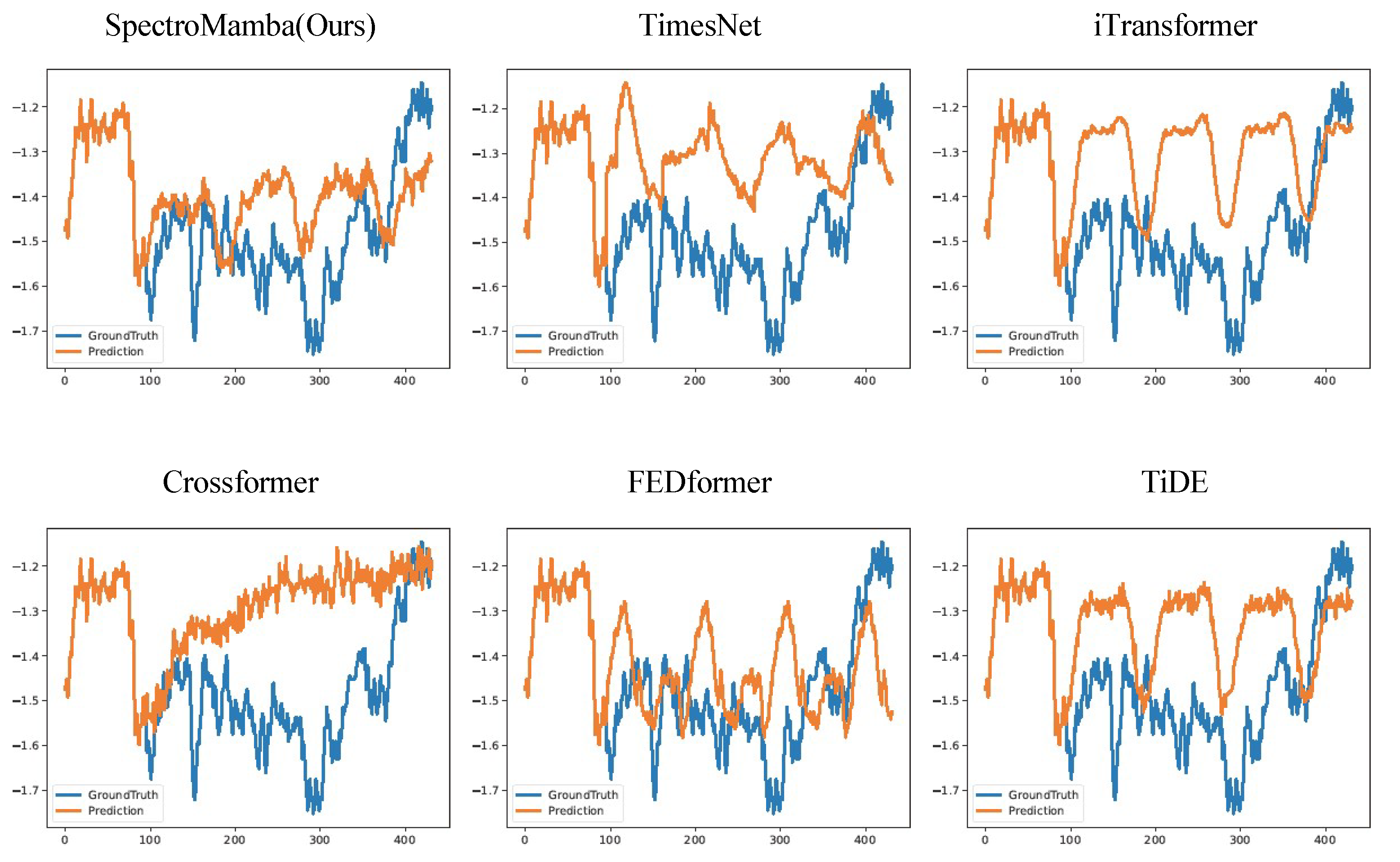
Figure 5.
Visualization of input-96-predict-720 results on the ETTm1 dataset.
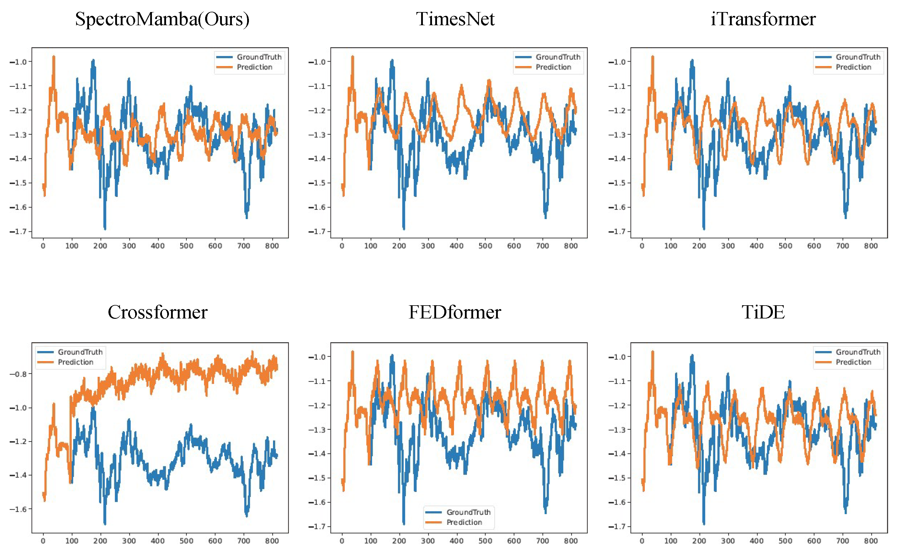
Figure 6.
Comparison of the average MAE performance across three runs on different datasets under varying noise levels.
Figure 6.
Comparison of the average MAE performance across three runs on different datasets under varying noise levels.
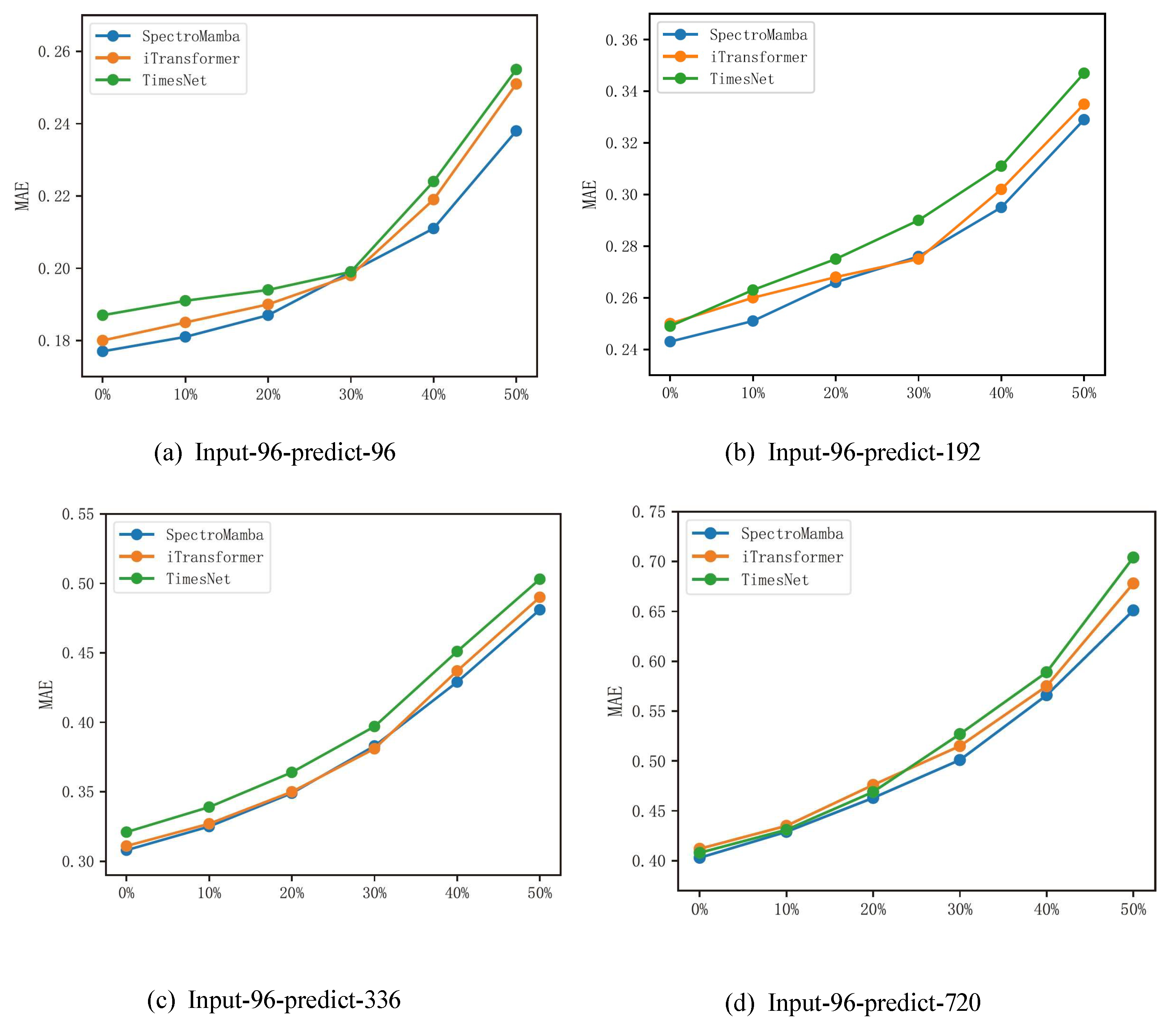

Table 1.
Long-term forecasting dataset description.
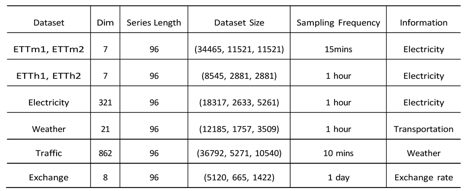
Table 2.
Full results of the long-term forecasting task. In accordance with the configuration of TimesNet , we compared widely competitive models at different prediction lengths. The input sequence length for all baseline models was set to 96. ”Avg” represents the average results across four different prediction lengths. A lower MSE or MAE indicates better prediction. The best result for each dataset is highlighted in bold red, while the second-best result is in bold with an underline.
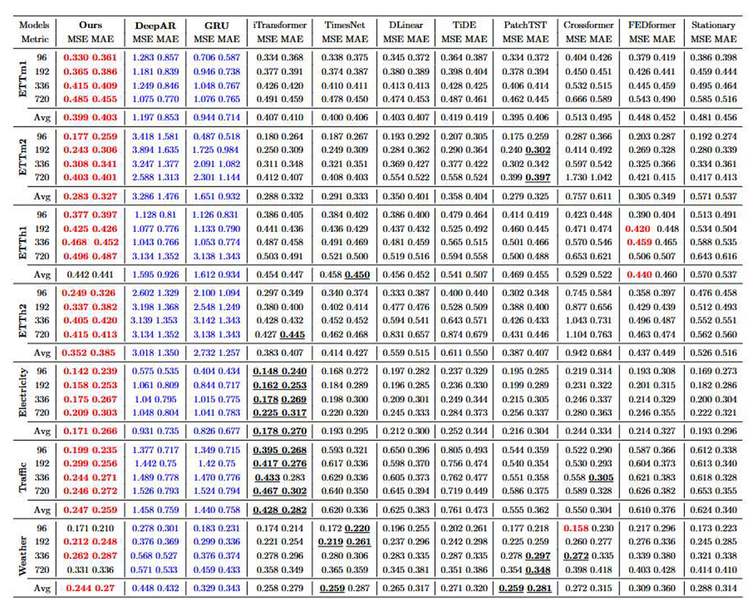
Table 3.
Ablation study of individual component.
Disclaimer/Publisher’s Note: The statements, opinions and data contained in all publications are solely those of the individual author(s) and contributor(s) and not of MDPI and/or the editor(s). MDPI and/or the editor(s) disclaim responsibility for any injury to people or property resulting from any ideas, methods, instructions or products referred to in the content. |
© 2025 by the authors. Licensee MDPI, Basel, Switzerland. This article is an open access article distributed under the terms and conditions of the Creative Commons Attribution (CC BY) license (http://creativecommons.org/licenses/by/4.0/).
Copyright: This open access article is published under a Creative Commons CC BY 4.0 license, which permit the free download, distribution, and reuse, provided that the author and preprint are cited in any reuse.


