
Submitted:
17 September 2025
Posted:
19 September 2025
You are already at the latest version
Abstract
Exposure to unexpected loads, aging material, and environmental conditions can trig-ger significant risks to the structural integrity of key infrastructures like bridges, buildings, and aircraft. Structural Health Monitoring approaches can be employed to understand and assess the condition of the structures in real time, helping detect damage and guide maintanance decisions. One of the biggest limitations of Structural Health Monitoring approaches is in predicting how a structure would respond under untested extreme loads. Conducting either physical testing or Finite Element Analysis for every possible scenario is time consuming and computationally expensive. The so-lution to this problem lies in surrogate finite element models, in which finite elements models are combined with machine learning approach to quickly and accurately evaluate structural vibrations for a wide range of conditions. Machine learning algo-rithms, capable of processing large datasets and identifying complex patterns, can be trained to model the behavior of structures subjected to time-varying loads. This study presents the experimental validation of surrogate finite element models constructed using artificial neural networks. These surrogate models provide mid-fidelity estimates of structural responses at arbitrary time instances and spatial locations during opera-tion. By learning the dynamic behavior of the structure, the surrogate is employed to develop a digital twin of the system. Experimental results confirm that the surrogate model improves the predictive accuracy of the baseline finite element model by incor-porating measurement data, thereby offering a robust representation of structural be-havior.
Keywords:
finite element
; machine learning
; vibrations
; artificial neural network
; structural health monitoring
1. Introduction
Data science models have revolutionized numerous sectors, including Finite Element Methods (FEM), which represent a fundamental tool in the analysis and solution of complex engineering problems [1]. Applying machine learning to FEM methods offers an innovative and promising perspective for improving the efficiency and accuracy of calculations and simulations in engineering domains.
The Finite Element Method (FEM) [2] provides an approximate solution to partial differential equations (PDEs) or integral equations by discretizing the domain of interest into finite elements. Its flexibility and ability to handle complex geometries and variable materials make it an essential analysis technique for many sectors, from structural component design to the simulation of complex physical phenomena. However, it is important to note that the accuracy of results obtained using FEM depends on the correct choice of finite element type, domain discretization, and the quality of the generated mesh. Generating an optimal mesh is a complex task and requires a significant amount of time and computational resources. Additionally, the approximate solution may be influenced by the numerical resolution used to solve the system of linear equations.
Applying machine learning in combination with FEM offers a promising solution to this challenge. With the ability to learn from large amounts of data and recognize complex patterns, machine learning algorithms can be trained to predict and automatically optimize the distribution of finite elements in the mesh. This allows for more accurate models, significantly reducing the time and effort required for mesh generation.
The state-of-the-art in applying machine learning to FEM is constantly evolving and sees numerous developments and interesting applications. Here are some of the highlights of the state-of-the-art in applying machine learning to FEM methods:
Learning material structure: Machine learning can be utilized to model and predict the properties of materials [3] used in FEM simulations, enabling a better understanding of their behavior and performance.
Reduction of computational cost: A significant area of interest is the reduction of computational cost associated with FEM simulation [4]. Machine learning can be employed to accelerate calculations or to develop reduced models that provide approximate results.
Design optimization: Machine learning can be applied to optimize the design of components or structures [5], enabling the discovery of better and more efficient solutions in terms of performance, strength, or weight reduction [6].
Modeling noise and vibrations: Machine learning can be used to model and predict the noise and vibrations generated by a system [7] allowing for better design and optimization of acoustic performance.
Data analysis and prediction: Machine learning can be deployed to analyze large amounts of data generated by FEM simulations, extract useful information such as performance prediction or design optimizations, identify patterns, and forecast the future behavior of analyzed systems.
Currently, one of the fields where machine learning algorithms have been applied to structures is civil engineering. Some studies [8] have focused on structural damage detection based on real-time vibration signals and convolutional neural networks, which are an advanced approach used to assess the structural health of buildings, bridges, and other infrastructures. This method utilizes vibration data acquired from sensors placed on the structure to identify any damages or anomalies.
Within civil engineering, the use of Machine Learning Models (MLMs) in combination with FEM is becoming more common. Jayasinghe S. et al. tested three MLMs, Random Forest, XGBoost algorithm, and Multi-Layer Perceptron (MLP) Neural Networks, for digital twin applications in SHM. The digital twin concept advances the traditional SHM systems while improving predictive maintenance and decision-making strategies by integrating the real-time monitoring data of infrastructure systems with their own digital models. When digital twins are combined with FEM, the capability is further expanded to predict critical stresses in real time and to immediately detect possible structural failures [9]. Another application of MLMs in SHM for bridge structures was investigated by Quan, E. and Li G. (2025). Using a Dynamic Bayesian Network (DBN), the researchers combined time series data and multi-source sensor information, finding the real time prediction of the bridge technical status and identifying the potential safety risks [10].
In the realm of civil engineering, similar MLM for SHM have been applied to port infrastructures. The use of Artificial Neural Networks (ANN) has been explored in combination with FEM for SHM of a conveyor carrying coal at the Dalrymple Bay Coal Terminal. The study developed a novel digital twin solution that incorporates ANN to assess its on-time structural behavior [11]. This study further solidified the use of FEM based digital twins in real-time monitoring of the structural response of infrastructure systems.
Beyond engineering, the applications of MLMs to further the impact of FEM in continuous health monitoring are abundant. Mao and Zhang (2025) explored the integration of the FEM with MLMs to expedite the diagnosis of human war related firearm injuries. Initially, the researchers established a FEM of the human lower limb bones based on CT images and validated material properties of the fibula and tibia. Subsequently, various combat scenarios under different loading conditions were simulated. Supervised machine learning algorithms, such as k-nearest neighbor (KNN), MLP, support vector machine(SVM), and random forest classifiers, were employed to classify wound characteristics.
Another study [12] has concentrated on the use of artificial neural networks for real-time prediction of structural stress through structural vibration tests. Zhiqiang et al. [8] estimate the stress in a structure utilizing vibration data acquired from sensors placed on the structure, with the objective to propose an alternative approach to visual inspection methods, which require a considerable amount of time to identify superficial damages. Initially, the authors considered natural frequencies and mode shapes as damage indicators. However, these indicators were limited due to the influence of the measurement environment.
Several classical machine learning algorithms have been used in various studies, such as Support Vector Machine, Decision Trees, and Artificial Neural Networks (ANN). Previous research shows that support vector and decision trees methods have good generalization capability and can handle non-linear data; however, in complex situations and with large-scale samples, they were found to be difficult to implement [8,12,13].
Finally, as advanced tools for data analysis, artificial neural networks could automatically extract information regarding structural damages present in signals and represent this information through the mapping of structural damage states. Other researchers explored the use of convolutional neural networks (CNNs) to detect damage based on FEA information and vibration measurements [13]. CNNs are effective in localizing and quantifying structural damage when the damage exceeds 10%.
ANNs have the potential to significantly accelerate forward calculation process and provide a more efficient approach to inverse analysis. Predicting stress or displacements has been the most common primary goal of most studies with a particular emphasis on addressing static structural behavior [14]. Another major advantage of neural networks is their ability to model and predict complex nonlinear relationships within the data. Neural networks stand out from traditional approaches in the prediction of complex structural systems’ behavior under variable loads [15].
ANNs can be also trained using measured system responses [16]. However, this requires a considerable amount of data as the performance of the ANN model improves when the number of frequency steps used during experiments increases. The approaches therefore required an excessive amount data to learn, leading to longer simulations and difficulty in obtaining enough data to compose the dataset [16,17].
Hybrid approaches have been proposed to combine machine learning, FEM results and vibration measurements (Gao, Mosalam, Chen, Wang, & Chen, 2021) machine learning with vibration data were used to obtain approximate damage localization, while a FEM model updating approach was then used to identify the exact damage location, reaching an accuracy of about 80%.
Machine learning approaches have also been proposed to predict structural stresses by using FEA simulations to train either a random forest or artificial neural networks approaches, and then combining the trained model to experimental measurements in order to obtain more accurate and computationally inexpensive tracking of dynamic stresses in the structure [18]. A one-dimensional beam like structure was examined, where the average distribution of stresses was predicted real-time after learning data obtained from FEA simulations on beam stresses to find reasonably accurate solutions at various positions. The approach is characterized by its remarkable versatility, allowing for the use of a wide range of response variables (such as displacement, velocity, acceleration, deformation, and stress) for training and prediction purposes [18,19,20].
Furthermore, for the detection of acceleration data on the structure, sensors are used, and machine learning has also been applied to define the best sensor position to monitor a vibrating system to detect the structure’s health status [21,22]. This methodology can be applied to any sensor and dynamic system to increase accuracy and reduce the number of redundant sensors.
In this paper, the experimental validation of the procedure introduced in [18] is presented. After a brief explanation of the proposed approach, experimental results for a one-dimensional structure is reported.
2. Materials and Methods
The goal of the approach is to create a surrogate finite element that provides a mid-fidelity estimate of the response of the system at any instant of time during operations, and at any locations of interest. To achieve this objective, the following sequence of steps is adapted from [18]:
- Construct a finite element model of the system of interest; run a series of time-varying FEA simulations to create a sufficiently large training dataset that represents the expected loading conditions.
- Use the results of FEA simulations to construct a training dataset and that will use to train the neural network. The training dataset contains, as inputs, the geometrical coordinates at which the output needs to be calculated as well as the numerical accelerations in correspondence of the experimental sensors (reference points). The output of the training dataset corresponds to the desired quantity in the system, i.e., the stress, or displacement, or acceleration.
- Train the ML algorithm to establish a relationship between the inputs and the output. This step establishes a relationship between the desired quantity (i.e., acceleration) at each nodal location in the finite element with the numerical response at a few nodal locations (reference points).
- Measure the response of the system and build an evaluation dataset that contains as inputs the coordinate x at which the output needs to be calculated as well as the data measured by the sensors at the reference points
- Apply the trained network model to the evaluation database to evaluate the corrected response at any nodal location in the system based on the measured quantities.
3. Experimental Validation on a Beam
The approach is initially validated on a one-dimensional aluminum cantilever beam measuring 175 mm in length, 19.16 mm in width, and 3.10 mm in thickness. A transverse time-varying load was applied through an electro-dynamic shaker at 0.105m from the clamp. A schematic of the physical system is presented in Figure 1.
The first step in the application of the approach is to model the beam using finite elements, which results are used to train the machine-learning model.
3.1. Experimental Setup
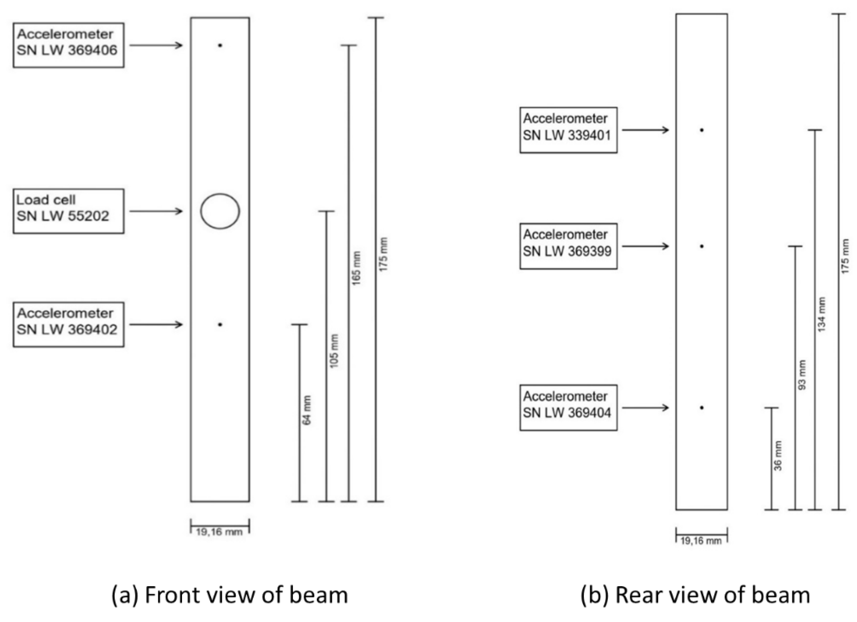
The experimental setup is depicted in Figure 3. The beam is clamped at the bottom with rigid blocks, and is excited by an electrodynamic shaker, with a load cell measuring the applied force. The response of the beam was measured with five accelerometers, positioned as in Figure 2 and Figure 3. The measured natural frequencies of the beam are listed in Table 2.
Figure 2.
Experimental setup of beam validation tests.
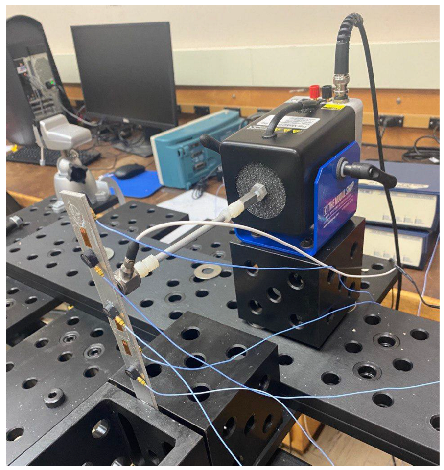
Figure 3.
Accelerometer positioning diagram on the beam.
Several tests were conducted to evaluate the performance of the algorithm, and each test excited the transverse deflection of the beam with broadband signals such as chirp and pseudorandom.
3.2. Beam Finite Element Model
The dataset to train the machine learning model is created using finite elements model of the beam. The transverse behavior of the beam is modeled with 50 Euler-Bernoulli beam elements, whose properties are listed in Table 1. The beam is clamped on one side, corresponding to Node 1. The mesh of the beam is shown in Figure 4.
Damping is introduced in the model in the form of proportional damping, with damping matrix and with coefficients and A transverse load is introduced in the model in correspondance of the position of the shaker (0.105m from the clamp).
The first three natural frequencies of the beam are listed in Table 2, and are compared to the measured natural frequencies. The maximum difference between the experimental and numerical natural frequencies is 5.3%, revealing a good correlation between the model and the experimental setup.
The numerical model was subjected to a variety of loads, which changed in amplitude, frequency and time variation. All the results were then combined in a dataset that was used to train a machine learning model.
3.3. Characteristic of dataset
For each case that needs to be analyzed, two different datasets are created: a training dataset that includes all the information of the numerical model on which the neural network is trained and an evaluation dataset that includes the experimental measurements and allows us to obtain the “measured” deformed shape along the beam.
For each time step in the numerical model, the training dataset contains the coordinate at which the output needs to be calculated as well as the numerical accelerations in correspondence of the five accelerometers along the beam (). The desired output corresponds to the numerical acceleration at location . The training dataset comprises approximately one million entries.
Artificial neural networks are used to simulate the behavior of the system due to their flexibility and proven strength in previous publications [20]. The ANN model is constructed using the Keras libraries. The model uses ReLu activation function, with a learning rate of 10-3 and iterates for 50 epochs.
Once the neural network model has been trained, it is then applied to a second database (the evaluation database) that contains as inputs the coordinate x at which the output needs to be calculated as well as the data measured by the accelerometers. The output will then be calculated by the trained neural network model.
4. Results
For the test case on a cantilever beam, a chirp force with an amplitude of 0.05 V and a frequency of 2000 Hz was applied to the beam. The chirp signal is generated using the “chirp” function in Matlab. Several case studies are presented in the following:
- Case A: training dataset: numerical (FEM data), evaluation dataset: numerical (FEM data);
- Case B: training dataset: numerical (FEM data), evaluation dataset: experimental; the information from all 5 accelerometers is used to train the ANN model;
- Case C: training dataset: numerical (FEM data), evaluation dataset: experimental; the information from 4 accelerometers is used to train the ANN model; the ANN prediction of one accelerometer is used to compare to the experimental data (one control point).
Case A is helpful to establish the capability of the ANN model to predict the overall numerical acceleration along the beam; the ANN model performs really well, with both training and predicting R2~0.99. The training mean absolute and square errors (Figure 5) converge well.
The acceleration along the beam predicted by the ANN model (Figure 6 – blue line) is also able to well represent the accelerations at the reference points (black stars). The numerical to numerical predictions therefore show that the ANN model is a solid representation of the numerical model of the beam.
The next step is to use the trained model to predict the acceleration along the beam by using the experimental measurements. For Case B, the ANN model is trained using five reference points as input, in correspondence of the five accelerometers. The ANN model is then tested using the measurements from five accelerometers as input. Figure 7 compares the acceleration along the beam at different time instants. The blue line represents the initial numerical response of the system before ANN were applied, the orange line represents the estimated response of the system after ANN were applied and the black dots represent the experimental measurements at each accelerometer. Initially, the deformed shape of the numerical model (blue line) shows large difference with the experimental measurements. The deformed shape evaluated by the ANN (orange lines) offers great improvements with respect to the measurement across the entire beam, therefore demonstrating that the ANN approach greatly improves the prediction of the system.
The time histories at different accelerometers’ locations also show an improvement with respect to the initial FEM predictions (Figure 8, Figure 9 and Figure 10). Figure 8 presents the full time histories at accelerometer p4, while Figure 9 and Figure 10 depict a detail of the time histories at accelerometer p4 and p5 respectively. Initially, the predictions of the acceleration by the FEM model are completely different than the experimental measurements, both in terms of absolute value and frequency of oscillation. The application of the ANN model corrects these errors and results in predictions that have similar phase and frequency as the experimental measurements of the accelerometer.
In case C, the ANN model is trained using numerical data at four reference points, excluding the information of reference point p4. As a result, the prediction of the ANN model will not require the knowledge of the measurement at accelerometer 4, which will be considered as a control point since its information was not used to generate the ANN predictions. Figure 11 compares the acceleration along the beam at different time instants for case C. The blue line represents the initial numerical response of the system before ANN were applied, the orange line represents the estimated response of the system after ANN were applied and the black dots represent the experimental measurements at each accelerometer. Initially, the deformed shape of the numerical model (blue line) shows large difference with the experimental measurements, similarly to ure 7. The deformed shape evaluated by the ANN (orange lines) offers great improvements in its ability to predict an acceleration distribution more similar to the experimental results.
5. Conclusions
The obtained results have indicated a significant convergence between the measured real accelerations and those predicted by ANN models. The analysis of discrepancies highlighted a substantial reduction in predictive errors, demonstrating the models’ ability to generalize and learn complex patterns in structural dynamics. The experimental validation presented in this paper shows that the ANN model can improve the prediction of the overall dynamic response of the beam with respect to an initial FEM prediction based on experimental measurements at few locations. Additionally, the possibility of obtaining excellent predictions using only 4 accelerometers instead of 5 suggests that the method is robust.
The practical implications of the conclusions reached extend to a wide range of sectors, from civil engineering to aerospace structures, where accurate prediction of structural accelerations is crucial for design and safety assessment. The use of ML models could simplify the structural analysis process, reducing dependence on computationally intensive FEM models and allowing for rapid performance evaluation and structural health monitoring in real-world scenarios. In conclusion, the application of machine learning methods in the analysis of structural accelerations has proven to be a promising prospect to model-based engineering. Integrating these approaches with traditional methodologies, such as finite elements, could represent the future of structural engineering, improving prediction accuracy and accelerating evaluation times.
Author Contributions
Conceptualization, M.C.; methodology, M.C.; software, S.A and A.R.; validation, S.A, M.C. and A.R.; formal analysis, S.A and A.R.; resources, M.C.; data curation, A.R.; writing—original draft preparation, S.A, M.C. and A.R.; writing—review and editing, S.A. and M.C.; supervision, M.C.; All authors have read and agreed to the published version of the manuscript.
Funding
This research received no external funding
Conflicts of Interest
The authors declare no conflicts of interest.
References
- R. E. Meethal, K. A. M. R. E. Meethal, K. A. M. Khalil, A. Ghantasala, B. Obst, B. K. and R. Wüchner, “Finite element method-enhanced neural network for forward and inverse problems,” Advanced Modeling and Simulation in Engineering Sciences, vol. 10, no. 6, 2023.
- W. Kam Liu, S. W. Kam Liu, S. Li and H. Park, “Eighty years of the finite element method: birth, evolution, and future,” Archives of Computational Methods in Engineering, vol. 29, p. 4431–4453, 2022.
- Y. Liu, T. Y. Liu, T. Zhao, W. Ju and S. Shi, “Materials discovery and design using machine learning”,” Shanghai University, Shanghai, 2017.
- J. Javier Naranjo-Perez, M. J. Javier Naranjo-Perez, M. Infantes, J. F. Jimenez-Alonso and S. Saez, “A collaborative machine learning-optimization algorithm to improve the finite element model updating of civil engineering structures,” Seville, 2020.
- S. Le Clainche, E. S. Le Clainche, E. Ferrer, S. Gibson, E. Cross, A. Parente and R. Vinuesa, “Improving aircraft performance using machine learning: a review,” Madrid, 2022.
- Y. Wang, C. Y. Wang, C. Soutis, D. Ando, Y. Sutou and F. Narita, “Application of deep neural network learning in composites design,” European Journal of Materials, vol. 2, no. 1, p. 117–170, 2022.
- B. Zaparoli Cunhaa, C. B. Zaparoli Cunhaa, C. Drozc, A. Zined, S. Foulard and M. Ichchoua, “A review of machine learning methods applied to structural dynamics and vibroacoustic,” Lyon, 2023.
- T. Zhiqiang, S. T. Zhiqiang, S. Z, J. C., G. C and Fangsen, “Structural Damage Detection Based on Real-Time Vibration Signal and Convolutional Neural Network,” Guangzhou, 2020.
- S. M. M. A. A. S. A. S. Z. S. F. S. S. &. T. J. Jayasinghe, “Application of machine learning for real-time structural integrity assessment of bridges.,” MDPI, 2025.
- E. Quan and G. Li, “Real-time prediction method of bridge technical status in complex environment based on dynamic Bayesian network,” Intelligent Decision Technologies, 2025.
- S. M. M. S. A. N. T. M. A. A. M. S. S. F. S. Z. &. S. S. Jayasinghe, “Innovative digital twin with artificial neural networks for real-time monitoring of structural response: A port structure case study.,” Ocean Engineering, 2024.
- M. Döhler, F. M. Döhler, F. Hille, L. Mevel and W. Rücker, “Structural health monitoring with statistical methods during progressive damage test of S101 Bridge,” Engineering Structures, vol. 69, pp. 183-193, 2014.
- S. Cofre-Martel, P. S. Cofre-Martel, P. Kobrich, E. Lopez Droguett and M. V., “Deep Convolutional Neural Network-Based Structural Damage Localization and Quantification Using Transmissibility Data,” Santiago, Chile, 2019.
- S. C. M. M. A. A. S. A. S. F. S. Z. T. J. &. S. S. Jayasinghe, “A review on the applications of artificial neural network techniques for accelerating finite element analysis in the civil engineering domain.,” Computers & Structures, 2025.
- R. Saini, “A review on artificial neural networks for structural analysis.,” Journal of Vibration Engineering & Technologies, 2025.
- L. Wilmes, R. L. Wilmes, R. Olympio, K. M. de Payrebrune and S. M., “Structural Vibration Tests: Use of Artificial Neural Networks for Live Prediction of Structural Stress,” Kaiserslautern, Germany, 2020.
- J. Pal, S. J. Pal, S. Sikdar, S. Banerjee and P. Banerji, “A Combined Machine Learning and Model Updating Method for Autonomous Monitoring of Bolted Connections in Steel Frame Structures Using Vibration Data,” Hamirpur, India, 2022.
- M. Chierichetti, F. M. Chierichetti, F. Davoudi Khakhi, Huang D. and P. Vurturbadarinath, “Surrogated finite element models using machine learning,” in AIAA Scitech 2021 Forum, Virtual Event, 2021.
- S. Choppala, T. S. Choppala, T. Kelmar, M. Chierichetti, F. Davoudi Khakhi and D. Huang, “Optimal sensor location and stress prediction on a plate using machine learning,” in AIAA SCITECH 2023 Forum, National Harbor, MD, 2023.
- P. Vurtur Badarinath, M. P. Vurtur Badarinath, M. Chierichetti and F. Davoudi Kakhki, “A machine learning approach as a surrogate for a finite element analysis: Status of research and application to one dimensional systems,” Sensors, vol. 21, no. 5, p. 1654, 2021.
- S. Arunachalam and M. Chierichetti, “A Sensor Placement Approach to Monitor Vibrations Based on Data-Driven Principal Component Analysis Techniques,” in ASME Aerospace Structures, Structural Dynamics, and Materials Conference, Houston, TX, 2025.
- T. Kelmar, M. T. Kelmar, M. Chierichetti and F. Davoudi Kakhki, “Optimization of sensor placement for modal testing using machine learning,” Applied Sciences, vol. 14, no. 7, p. 3040, 2024.
Figure 1.
Schematic of physical beam.
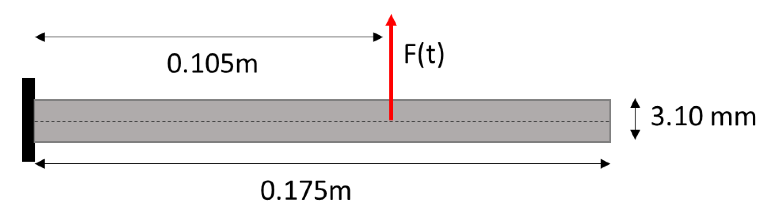
Figure 4.
Mesh of the beam FEM.
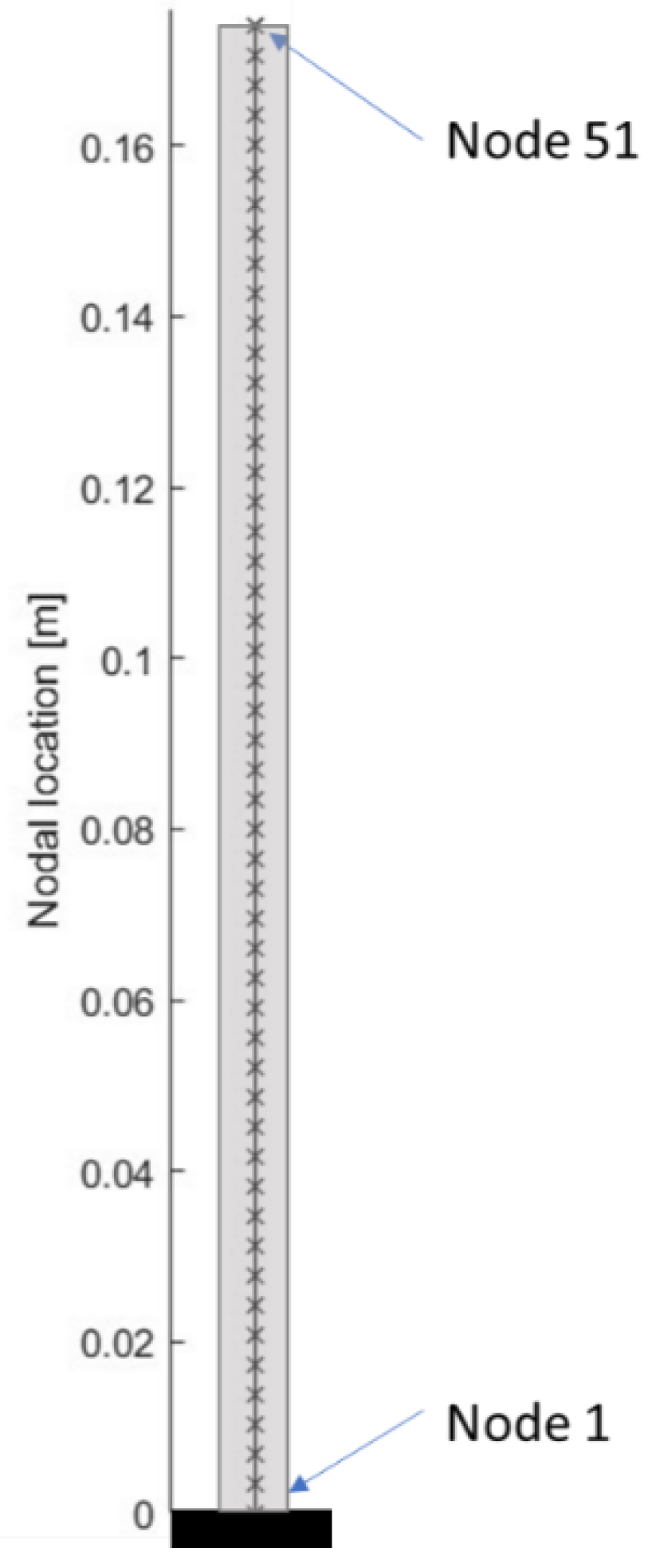
Figure 5.
Training mean absolute and square errors for case A.
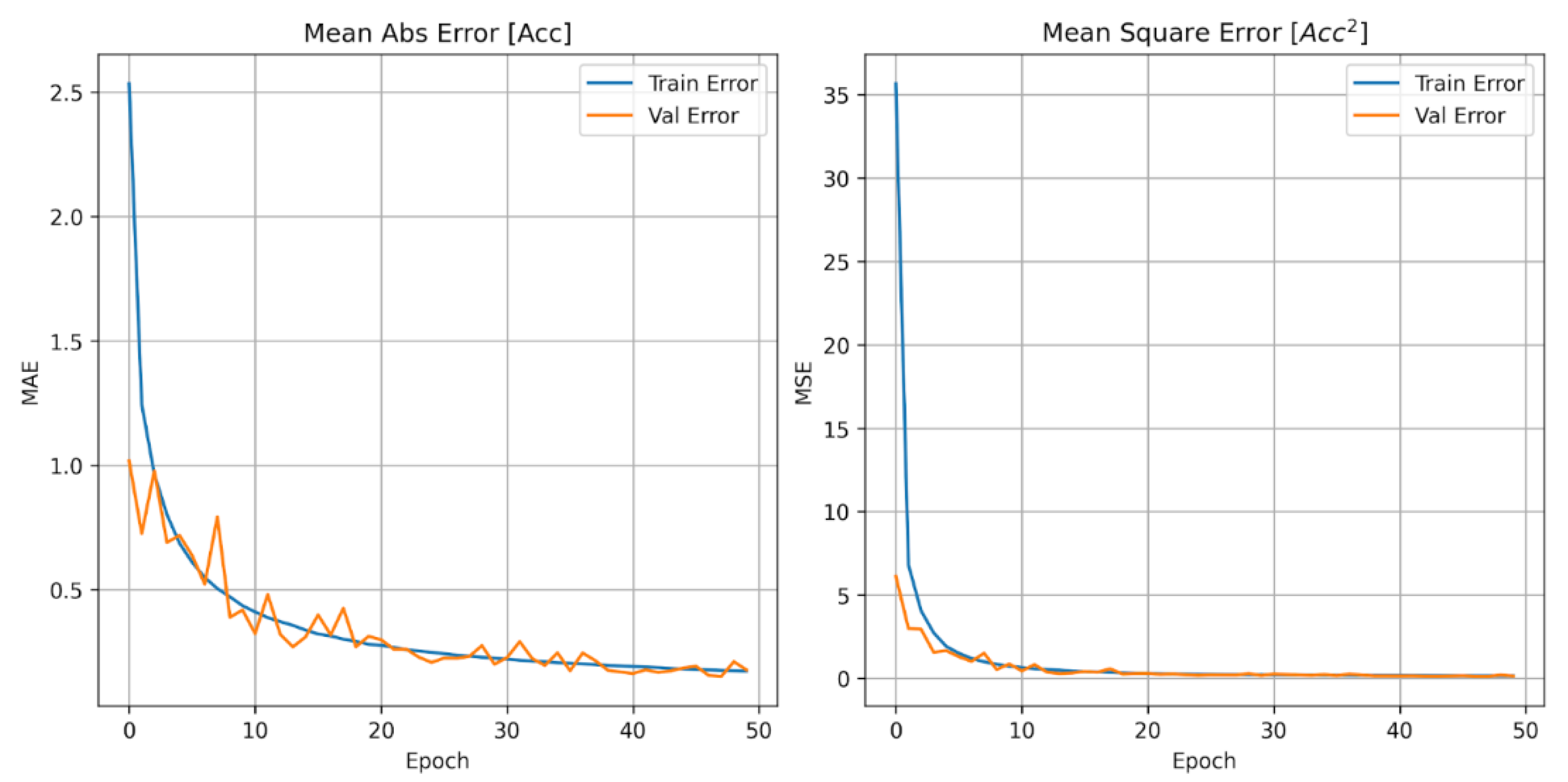
Figure 6.
Acceleration along the beam at different time instants –Time=0.5 s & Time=2.0 s, case A.
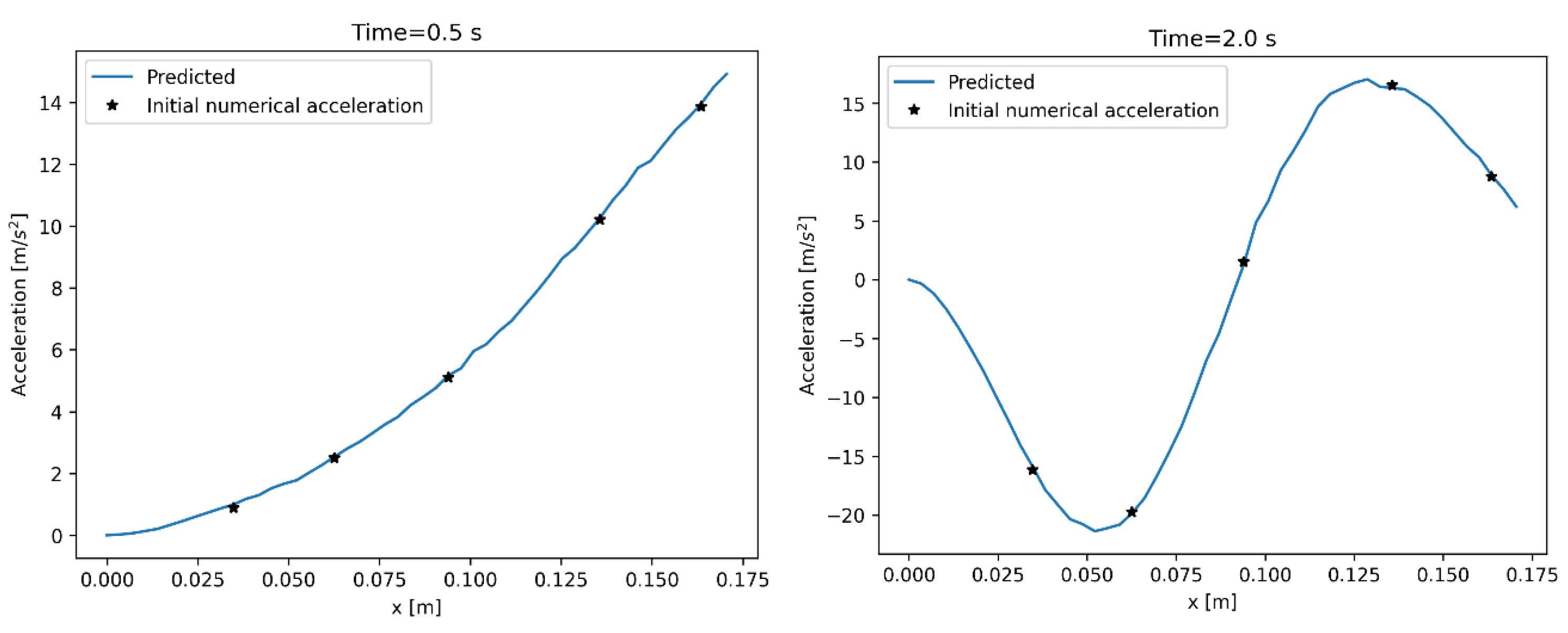
Figure 7.
Acceleration along the beam at different time instants – Time=0.5 s & Time=1.0 s & Time=2.0 s & Time=3.0 s, case B.
Figure 7.
Acceleration along the beam at different time instants – Time=0.5 s & Time=1.0 s & Time=2.0 s & Time=3.0 s, case B.
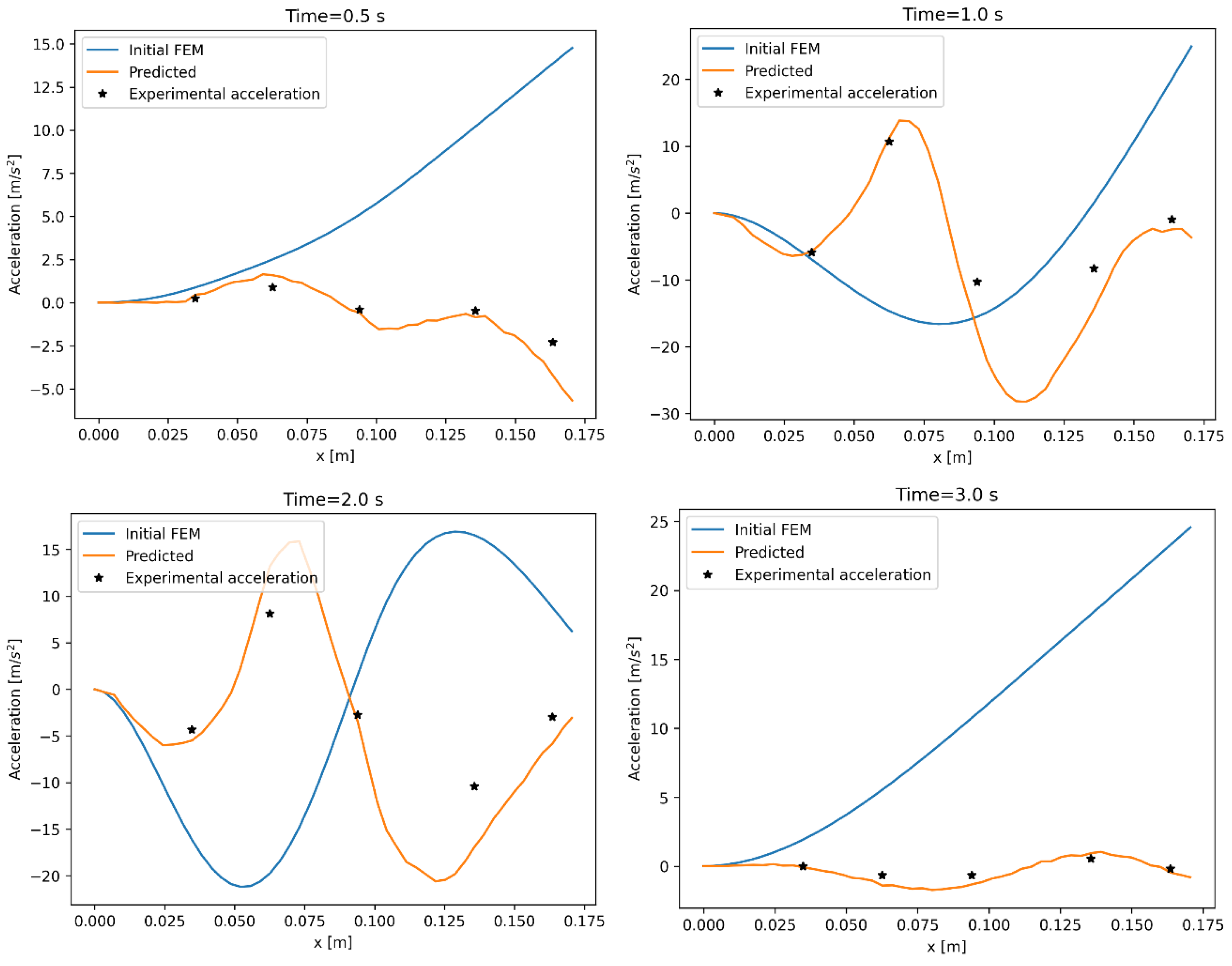
Figure 8.
Time histories at accelerometer p4, case B. FEM vs measurement (left), ANN prediction vs measurement (right).
Figure 8.
Time histories at accelerometer p4, case B. FEM vs measurement (left), ANN prediction vs measurement (right).
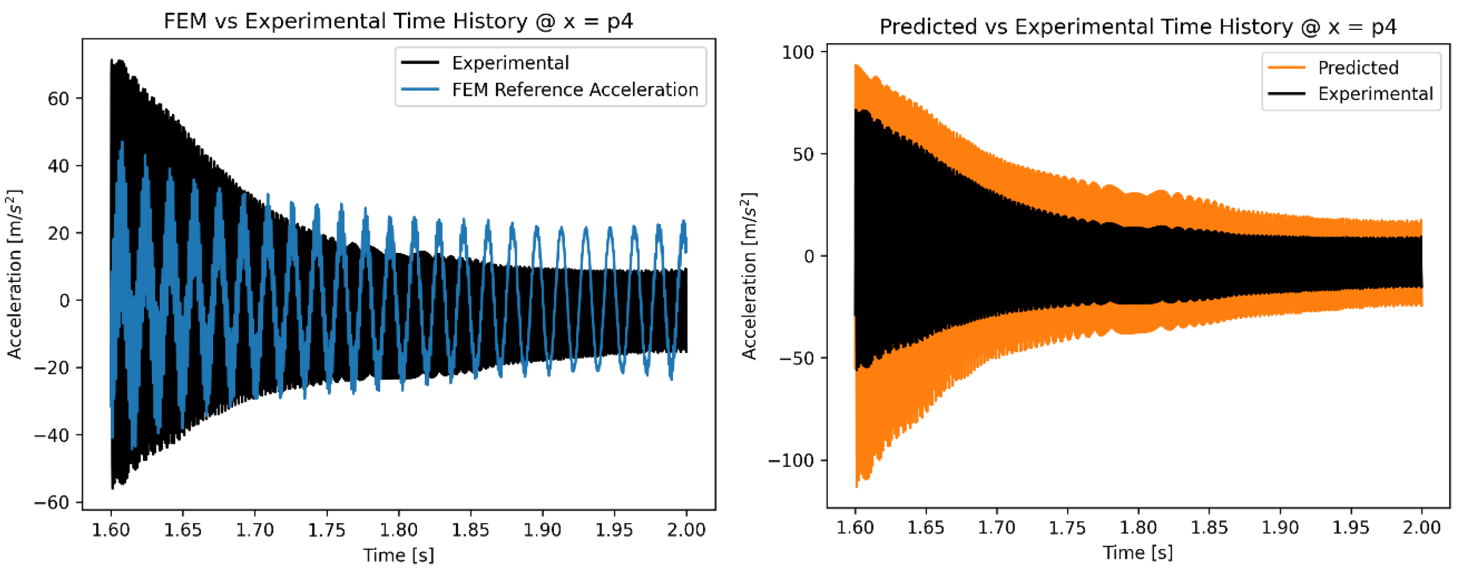
Figure 9.
Detail of the time histories at accelerometer p4, case B.
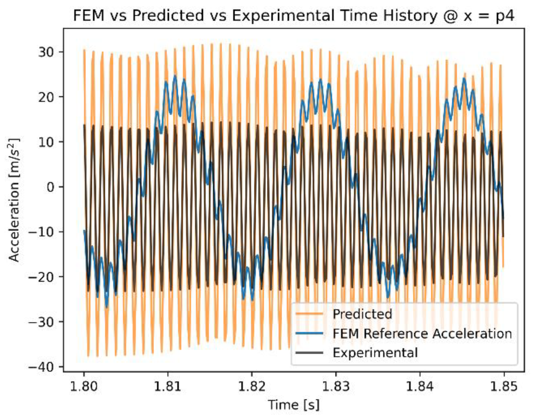
Figure 10.
Detail of the time histories at accelerometer p5, case B.
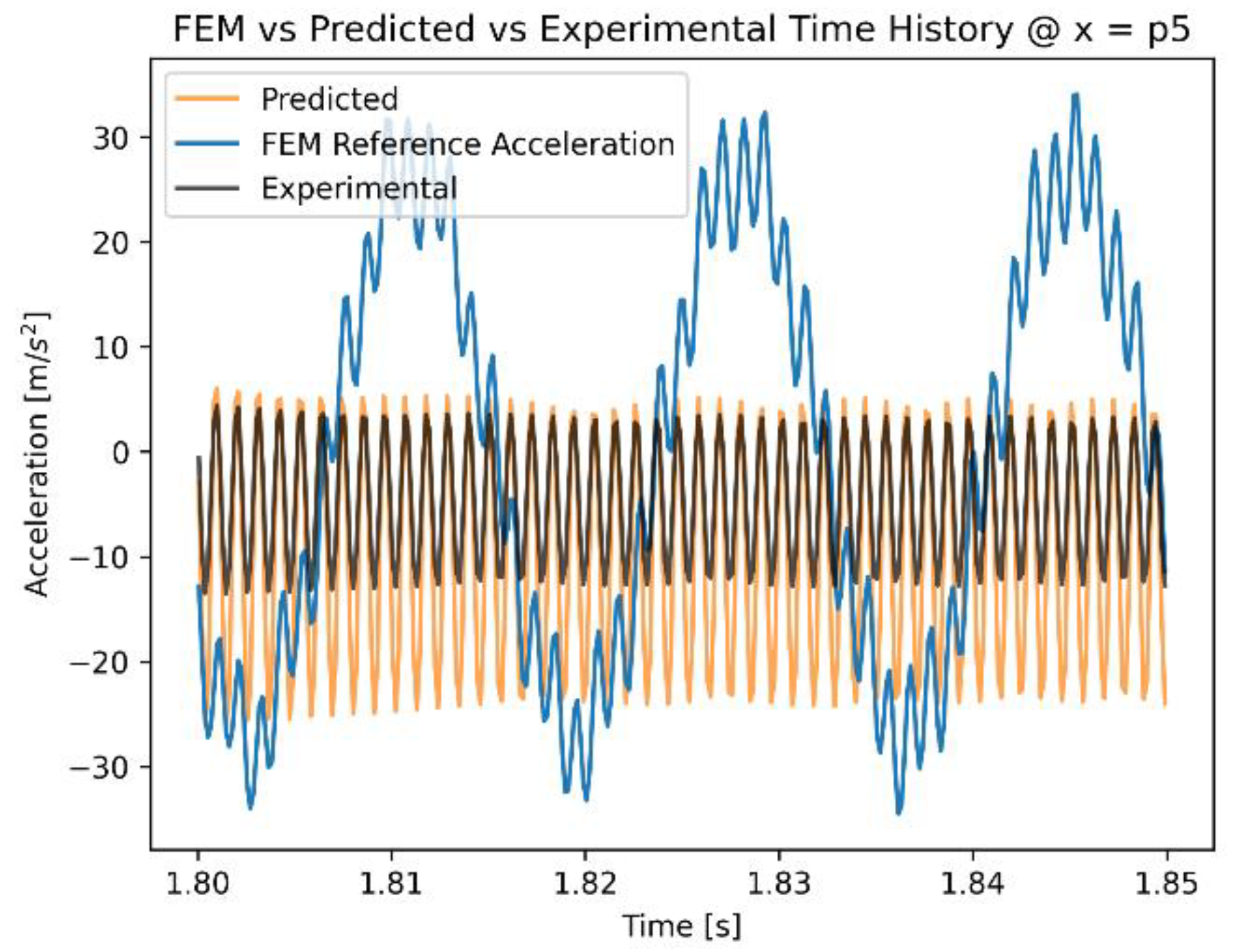
Figure 11.
Acceleration along the beam at different time instants – Time=0.5 s & Time=1.0 s & Time=2.0 s & Time=3.0 s, case C.
Figure 11.
Acceleration along the beam at different time instants – Time=0.5 s & Time=1.0 s & Time=2.0 s & Time=3.0 s, case C.
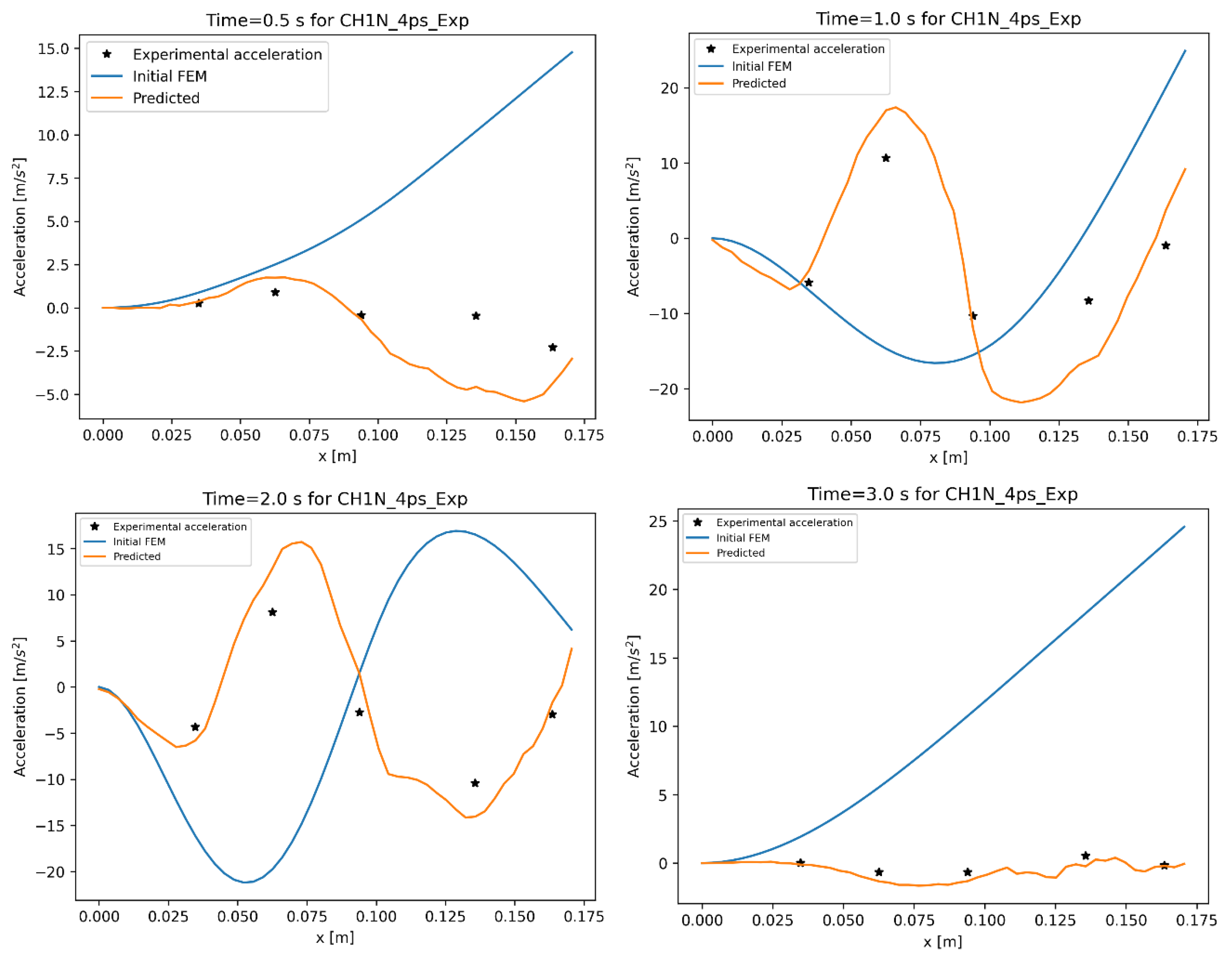
Figure 12.
Time histories at accelerometer p4, case C. FEM vs measurement (left), ANN prediction vs measurement (right).
Figure 12.
Time histories at accelerometer p4, case C. FEM vs measurement (left), ANN prediction vs measurement (right).
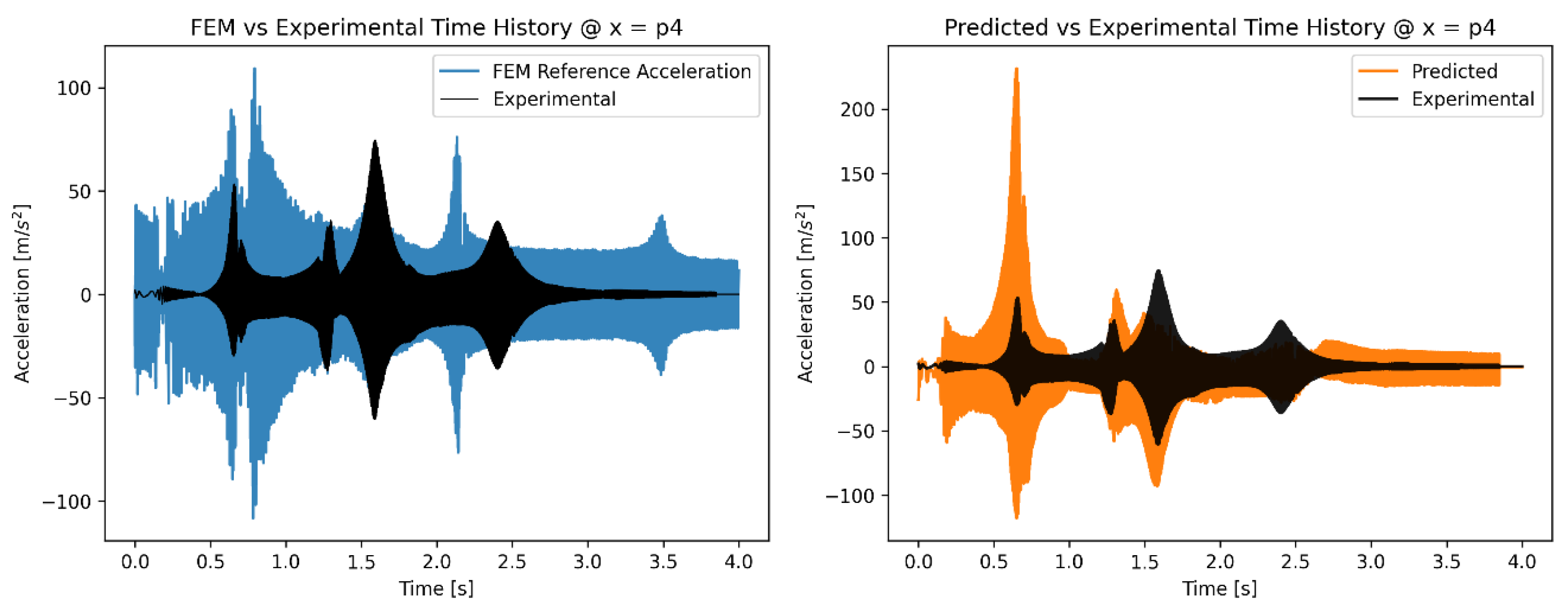
Figure 13.
Detail of the time histories at accelerometer p4, case C.
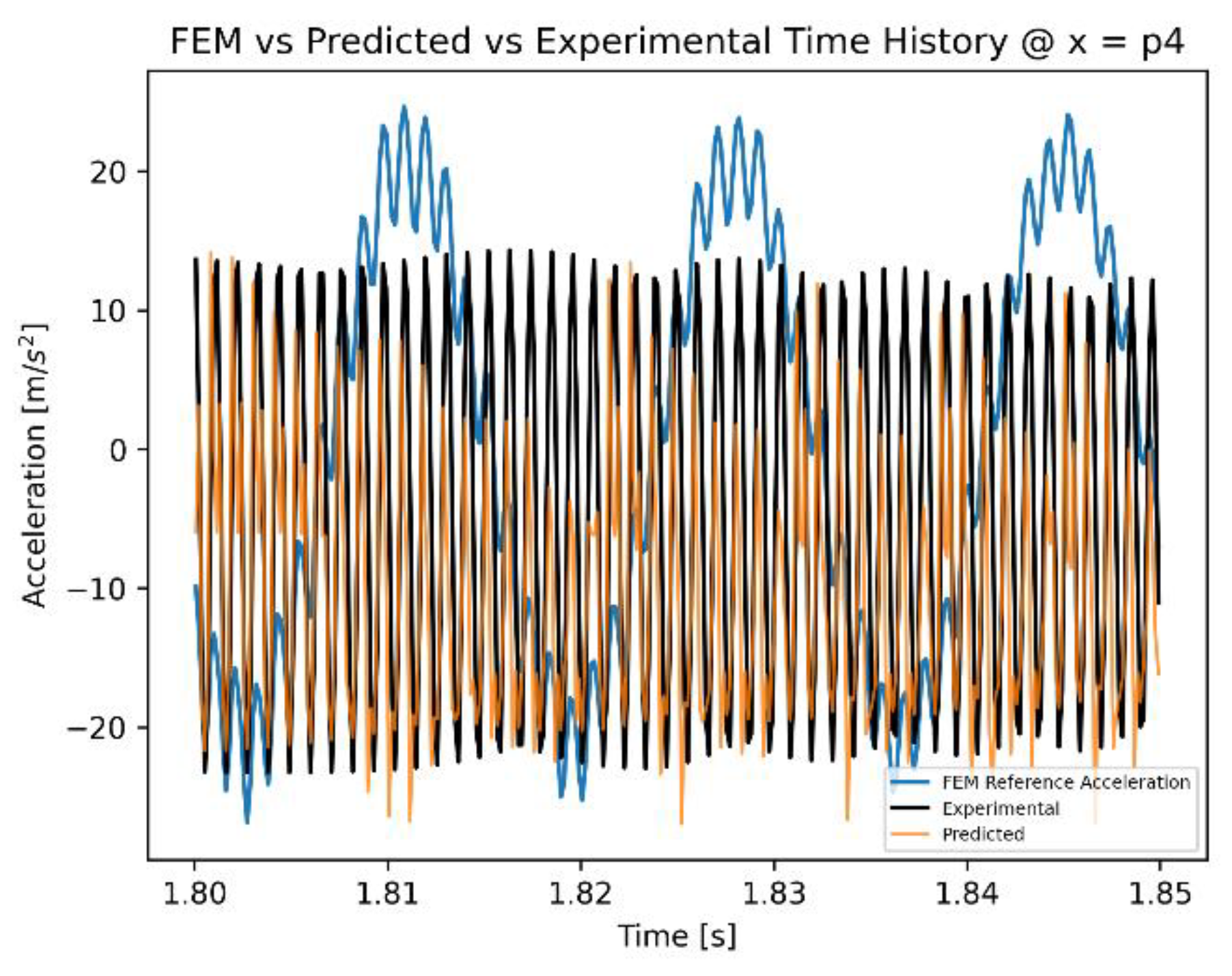

Table 1.
Cantilever beam properties.
| Property | Value |
|---|---|
| Length | 0.175 m |
| Width | 0.0192 m |
| Thickness | 0.0031 m |
| E (Young’s modulus) | 60 GPa |
| (Poisson’s ration) | 0.33 |
| (density) | 2800 kg/m3 |
Table 2.
Natural frequencies of cantilever beam.
| Mode Number | Experimental natural frequencies (Hz) | FEA Natural Frequency (Hz) |
|---|---|---|
| 1 | 58.0 | 58.9 (1.5%) |
| 2 | 351.0 | 369.8 (5.3%) |
| 3 | 1245.7 | 1191.9 (4.3%) |
Disclaimer/Publisher’s Note: The statements, opinions and data contained in all publications are solely those of the individual author(s) and contributor(s) and not of MDPI and/or the editor(s). MDPI and/or the editor(s) disclaim responsibility for any injury to people or property resulting from any ideas, methods, instructions or products referred to in the content. |
© 2025 by the authors. Licensee MDPI, Basel, Switzerland. This article is an open access article distributed under the terms and conditions of the Creative Commons Attribution (CC BY) license (http://creativecommons.org/licenses/by/4.0/).
Copyright: This open access article is published under a Creative Commons CC BY 4.0 license, which permit the free download, distribution, and reuse, provided that the author and preprint are cited in any reuse.


