
Submitted:
17 September 2025
Posted:
19 September 2025
You are already at the latest version
Abstract
Objective: To analyze the temporal evolution and spatial distribution of classic and hemorrhagic dengue in the Mexican state of San Luis Potosí at the basic geostatistical area (BGA) level and to develop multivariate models to estimate the population’s degree of vulnerability. Methodology: Classic and hemorrhagic dengue cases for 2015–2020 were obtained from the Mexican Ministry of Health, georeferenced at the pixel level, and subsequently grouped by BGA. Environmental, proximity, and social variables were obtained from official sites: IMTA, SMN, USGS, and INEGI. Multivariate logistic regression models were developed using PASW Statistics v. 18 software to estimate the degree of vulnerability, and the receiver operating characteristic curve was used to validate them. Results: A total of 125, 128, 109, 624, 1,580, and 1,817 dengue cases were identified for 2015, 2016, 2017, 2018, 2019, and 2020, respectively. The major factors contributing to the vulnerability of classic dengue fever included population, temperature, and distance to agricultural areas. For hemorrhagic dengue, the contributing factors were temperature, population, and mean annual rainfall. Vulnerability prediction was determined by taking the area under the curve values, which were 0.957 for classic dengue fever and 0.930 for hemorrhagic dengue, both indicating a “very good ability” to predict. Conclusion: These results can be used to design and implement targeted strategies, particularly for modifiable factors, such as prevention measures directed towards populated areas and the improvement of sewage systems, in addition to non-modifiable factors, such as temperature and rainfall. This method can be replicated as an additional tool to address this public health issue.
Keywords:
dengue virus
; receiver operating characteristic curve
; spatial analysis
; geographic information system
; risk factors
1. Introduction
Dengue is an infectious viral disease caused by the dengue virus, of which there are four serotypes, and spread through mosquito bites [1]. Consequently, individuals can be infected up to four times. The primary vectors for this disease are Aedes aegypti mosquitoes, with Aedes albopictus playing a secondary role in transmission.
About half of the world’s population is at risk of contracting dengue, with between 100 and 400 million infections occurring annually. Although most people who contract dengue are asymptomatic, the disease can sometimes worsen, requiring hospitalization; in severe cases, it may be fatal [2].
In 2022, there were 2.8 million reported cases of dengue in the Americas, more than double the 1.2 million cases reported in 2021 [1]. In Mexico, 6,746 cases of dengue were reported in 2021; this number nearly doubled in 2022, reaching 12,671 cases [3]. Similarly, in the Mexican state of San Luis Potosí, 566 confirmed cases were reported in 2023, with 108 cases exhibiting severe to alarming symptoms [4].
Dengue primarily occurs in tropical and subtropical regions worldwide, particularly in urban and semi-urban areas [2]. However, studies have shown that the incidence in rural areas can equal or exceed that in urban regions [5]. Moreover, global warming is expected to increase dengue cases worldwide [6]. Various factors contributing to its spread include migratory movements, increased national and international trade, population growth, and unsustainable urbanization practices such as poor-quality housing and inadequate waste management systems, creating favorable conditions for vector breeding [7].
Relevant studies on dengue have used spatial and statistical modeling. [8] applied MaxEnt distribution modeling to predict dengue virus distribution, incorporating sociodemographic and housing data. [8] Analyzed the correlation between dengue incidences and socioenvironmental factors and the spatial behavior of dengue between 2011 and 2014, using Pearson’s coefficient and Kernel estimators for geospatial analysis. [10] examined the relationship between dengue epidemiology and meteorological factors to forecast case numbers and plan resource allocation, employing the autoregressive integrated moving average model at both national and state levels.
Dengue became endemic in Mexico during the 1980s, prompting governmental initiatives aimed at prevention and control through program implementation. However, these efforts were insufficient to curb the rise in cases, which spread to over 90% of the country’s states by 2000 [11]. Consequently, this study aims to develop geospatial and statistical models to estimate vulnerability to classic dengue and hemorrhagic dengue fever at the rural and urban basic geostatistical area (BGA) level in San Luis Potosí State, Mexico. It also seeks to assess these dengue types’ temporal evolution and spatial distribution at the BGA level, advancing multivariate models to determine population vulnerability.
2. Materials and Methods
2.1. Study Area
2.2. Available Data
Data were obtained from the Department of Health of the San Luis Potosí State Government [13], encompassing all cases of dengue that occurred between 2015 and 2020, comprising 4,180 cases of classic dengue fever and 203 hemorrhagic dengue cases. A total of 4,383 dengue cases were georeferenced using the UTM projection - zone 14. Precise geographic coordinates of each dengue case were obtained using Google Earth, Google Maps, Heraldo Maps, Roadmap, Satellite-Maps, Map-Carta, and postal code databases (Código.mx).
2.3. Variables
Four factors (environmental, proximity, location, and social) were considered independent variables contributing to the abundance of mosquitoes. All values were obtained at the pixel level (30 meters) across rural and urban areas and then grouped by rural and BGA. Environmental Variables: Elevations of all municipalities in San Luis Potosí were obtained using the INEGI Digital Elevation Model [14]. Temperature and rainfall data were gathered from all 83 weather stations in the state [15,16]. These values were interpolated using the inverse distance weighted algorithm to achieve their pixel-level values through rasterization. Humidity values were derived from the Climate Research Unit’s historical archives and interpolated using the ordinary Kriging method [17,18,19].
For proximity variables, the Euclidean distance algorithm was employed to determine proximity values to the nearest body of water, wooded areas, grasslands, agricultural areas, and roads or paths by calculating the metric distance from each pixel in the raster to its nearest location [20,21].
For land use mapping, a supervised classification using the maximum likelihood algorithm was performed on Landsat spectral data to extract bodies of water and wooded areas [22]. Landsat 8 Operational Land Imager images were downloaded from Glovis for scenes 028-043, 028-044, 028-045, and 029-044, with dates ranging from November 16, 2021, to December 25, 2021 [23]. These products underwent systematic geometric corrections, utilizing ground control points or shipboard position information to deliver images recorded in a map projection referenced to WGS84, G873, or its current version. Training fields were digitized from land use and land cover features over the imagery and supported by a land use/land cover map [21,24]. Following the Landsat-based spectral data classification, validation was conducted by constructing an error matrix using field control point data, achieving an overall accuracy of 95.38% and a Kappa of 0.91 [25].
Location Variables: To identify spatial trends in dengue outbreaks, the X and Y UTM coordinates (XUTM, YUTM) were used [26]. Horizontal (XUTM) and vertical (YUTM) sweeps were performed over the study area utilizing IDRISI Selva v.17.0 software, generating two raster-format files: XUTM and YUTM (Figure 2).
Social Variables: The population size affects the probability of contracting dengue [27]. Local population data were sourced from the 2020 Geostatistical Framework and interpolated using the ordinary Kriging method [28]. To explore social inequalities and their relationship to dengue vulnerability [29], data were gathered on two social variables indicating living conditions: the percentage of homes with piped water and those with drainage systems [30]. These indices were obtained by rasterizing municipal boundaries, using the index of interest as a pixel value (Table 1).
3. Methods
A database was constructed in Microsoft Access to develop the entity-relationship model, which includes all the tables that form the structure and are related through their primary keys, establishing a 1-to-many relationship. This model enabled the creation of a foreign key named the locality key, which is located within the table labeled ‘dengue.’ This table encompasses all the cases from the period 2015-2020, and through this key, was linked to the table containing all rural and urban localities of San Luis Potosi. Consequently, the coordinates for each dengue case were obtained (Figure 3).
A spatial resolution grid of 1,000 by 1,000 km was constructed, classifying 7,545 pixels. Within these pixels, the coordinates of 4,180 cases of classic dengue fever and 203 cases of dengue hemorrhagic fever were located, leaving 3,162 pixels without registered dengue cases. These were subsequently grouped by BGA. To assess vulnerability to dengue at the BGA level, which may be influenced by each independent variable individually, the 7,545 spatial units and all the dengue cases registered during the studied period were used.
The software Access, Excel, ArcMap 10.1, and PASW Statistics v. 18 were employed to estimate and compare the means, using one-way ANOVA, of the values of the independent variables among BGAs without dengue, BGAs with dengue hemorrhagic fever, and BGAs with classic dengue fever. A binary logistic regression was conducted; this statistical tool is appropriate when the dependent variable can have only two values: 1 when the condition is present and 0 when it is absent [34], with dengue cases as the dependent variable. The result in each model is expressed in terms of probability, ranging from 0 to 1, where 1 indicates the presence of dengue and 0 its absence (probability >0.5 for presence, and 0 for probability <0.5) [34].
Two multivariate binary logistic regression models were also developed, one for cases of classic dengue fever and the other for hemorrhagic dengue, to estimate dengue vulnerability at the BGA level, which may result from the collective influence of independent variables. The final models were refined by excluding independent variables exhibiting multicollinearity [35].
Multiple linear regression was utilized to validate the absence of multicollinearity [35], both for classic and hemorrhagic dengue, considering a variance inflation factor ≤10 as indicative of no multicollinearity [35]. The discriminative ability of the multivariate models was evaluated using the receiver operating characteristic curve. This statistical method is useful in determining the diagnostic accuracy of the models to estimate the probability of detecting true positives (sensitivity) versus false positives (1 - specificity) [37].
The area under the receiver operating characteristic curve is a measure that quantifies the goodness of fit for the models and was used as a potential predictive indicator, with values ranging between 0.5 and 1 [37]. Additionally, the optimal cut-off point was identified (i.e., the value with the highest sensitivity and the lowest number of false positives [1 = specificity]), for which the Youden index was employed [38]. The Kappa coefficient was applied to evaluate the concordance between recorded dengue cases and those estimated by the multivariate models [39].
The independent variables were transformed to a standardized scale to be comparable before performing the logistic regression [40]. The following expression was used:
, where Z and are the transformed and original explanatory variables, respectively, is the arithmetic mean, and S is the standard deviation. This approach facilitates identifying each variable’s impact on dengue vulnerability and aids in interpretation. To estimate dengue levels of risk and the percentage of the San Luis Potosi population potentially affected at the BGA level, the following five-level risk scale was used: very low (0–0.199), low (0.2–0.399), medium (0.4–0.599), high (0.6–0.799), and very high (0.8–1) [41].
4. Results
A sustained increase in dengue cases was found in each year of the period, except in 2017 (Figure 4).
Regarding the independent variables, more than 50% have a standard deviation greater than their respective means. Considering the mean and median, one can observe that, in the absence of dengue, the values are lower for the following variables: average annual temperature, average annual rainfall, and population. Conversely, the values are higher for the percentage of homes with piped water and those with drainage. For the remaining variables, a priori, it is not possible to specify any others. The reality is that the combination of these variable values can favor mosquito development (Table 2).
All independent variables (factors) demonstrated a statistically significant relationship with the two types of dengue, except for the variable ‘Elevation above sea level’ in hemorrhagic dengue. Aside from ‘Elevation above sea level,’ the beta coefficients for all environmental variables were positive, indicating that they are risk factors. In contrast, variables related to proximity had negative coefficients, suggesting that an increase in these variables leads to a decrease in risk. This is similarly observed for the percentage of homes with piped water and homes with drainage. Conversely, the variable ‘Population’ has a positive coefficient, indicating that as the population increases, so does the risk (Table 3).
Table 4 reveals that the variable distance to agricultural areas was not statistically significant, whereas eight variables were not significant for dengue hemorrhagic fever. However, both models indicated multicollinearity among several factors, such as distance to roads for classic and hemorrhagic dengue fever.
When variables that exhibited multicollinearity were excluded from the models, all variables were statistically significant in both types of dengue. In both models, the signs of the beta coefficients align with theoretical expectations; an increase in variables with negative beta coefficients indicates a decreased risk of contracting dengue, while those with positive coefficients increase it. Additionally, the omnibus tests for classic and hemorrhagic dengue showed p < 0.001, allowing us to interpret the logistic model. This suggests that at least one is significantly different from zero among all the model coefficients.
The models with standardized variables identified the same three risk factors for vulnerability to classic and hemorrhagic dengue. The most significant factor for hemorrhagic dengue was the mean annual temperature at the BGA level, whereas for classic dengue fever, it was the second most significant factor. Significant differences were observed in the means and medians, which were lower in BGAs without dengue, followed by BGAs with hemorrhagic dengue, and finally, those with classic dengue fever. The mean and median temperatures of BGAs with dengue were 22.9 and 24.2 °C, respectively, with minimum and maximum temperatures ranging from 16.8 to 27.1 °C.
The population of the BGA is the primary factor for classic dengue fever and the third for hemorrhagic dengue. Increasing population density heightens vulnerability because an infected female mosquito is more likely to infect additional individuals. Similarly, rainfall was identified as the second most significant factor for hemorrhagic dengue and the third for classic dengue fever (Table 5).
The Kappa test result, assessing the concordance between BGAs with registered cases and those without versus the presence or absence of dengue estimated by the models for the same BGAs, showed a Kappa coefficient of 0.791 (p < 0.001) for classic dengue fever and a Kappa of 0.459 (p < 0.001) for dengue hemorrhagic fever. Over 50% of the population was identified as having high risk (Table 6).
Figure 5 illustrates that the area under the curve demonstrates a strong ability to correctly distinguish whether a particular BGA has dengue, with values of 0.957 (a) for classic dengue fever and 0.930 (c) for hemorrhagic dengue. In both instances, the confidence interval does not include 0.5, indicating a significant difference in the BGAs susceptible to dengue. The optimal point where sensitivity and specificity are maximized is 0.975 sensitivity and 0.816 specificity for classic dengue fever. For hemorrhagic dengue, these values are 0.926 and 0.768, respectively. Furthermore, the optimal decision threshold for BGA accurately identifying a BGA as having a true positive or true negative result was determined to be (0.184, 0.957) for classic dengue fever (b) and (0.232, 0.926) for hemorrhagic dengue (d). At these thresholds, the maximum difference between sensitivity and 1-specificity was noted.
Figure 5.
ROC Curve.
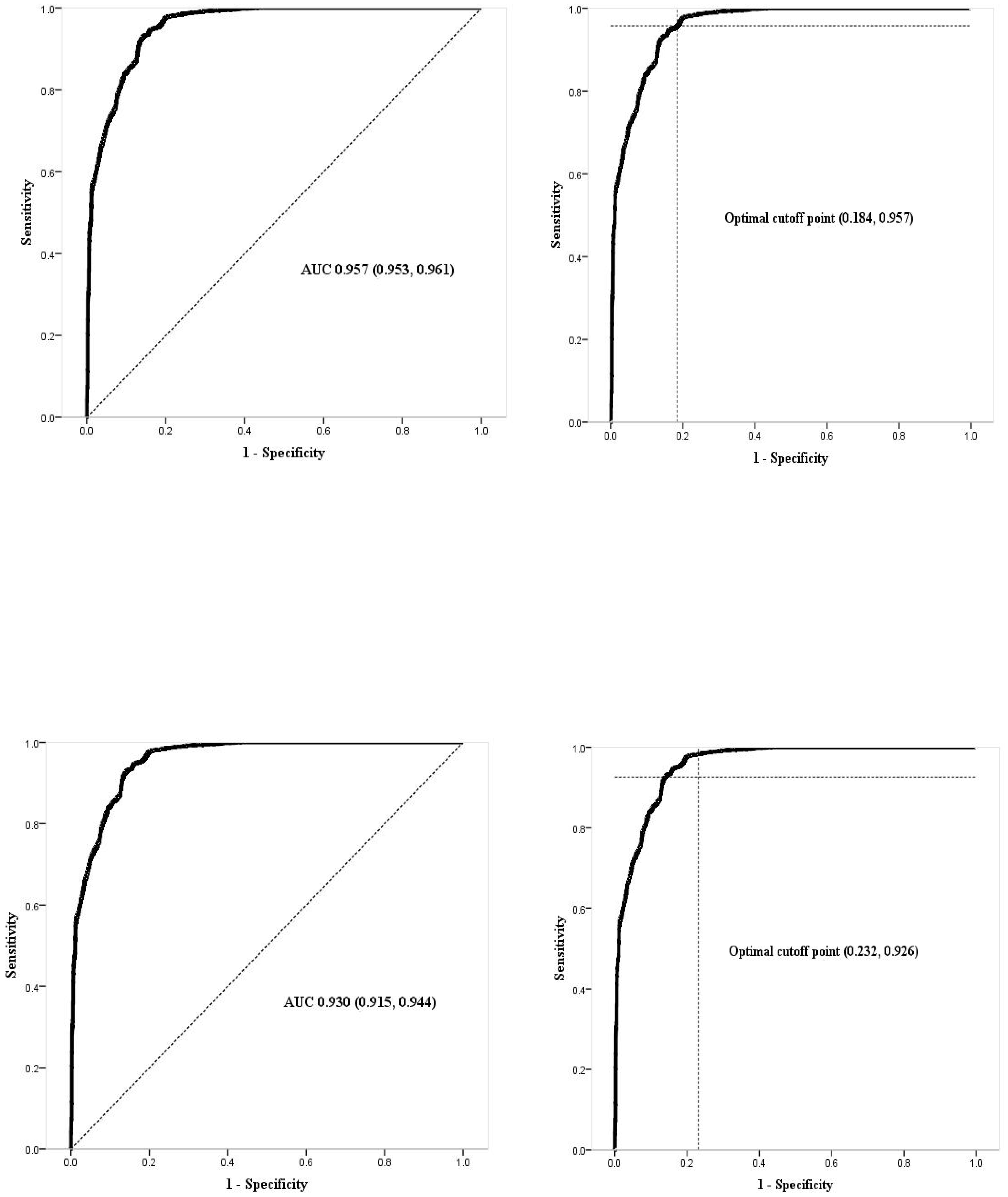
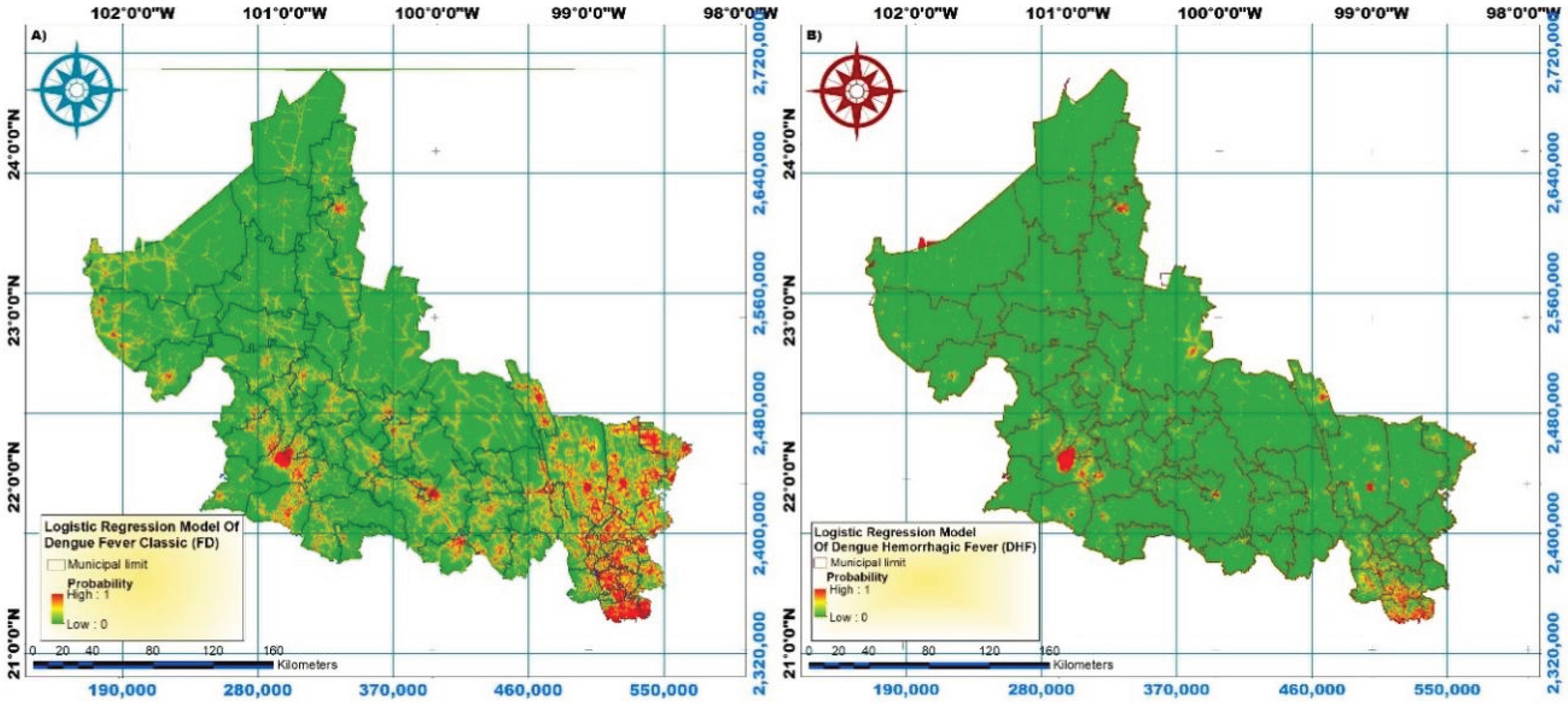
Figure 6.
Classic and hemorrhagic dengue fever spatial distribution.
5. Discussion
In this study, 13.7% of classic dengue cases and 27.6% of hemorrhagic dengue cases occurred in the desert and colder areas of the central and northern parts of the state, where dengue had not previously been reported. This shift is attributed to changes in infection patterns. As [42], noted, these changes are driven by extreme meteorological phenomena, climate change, and the El Niño phenomenon, in conjunction with the adaptive capacity of mosquitoes [43].
The Huasteca region features characteristics conducive to the proliferation of the Aedes aegypti mosquito, with climates ranging from warm-humid and warm subhumid to temperate-humid. Temperatures can fluctuate between 50 °C and -2 °C, and rainfall is abundant [44]. Several factors contributing to this health problem is interrelated, such as rainfall and humidity [1,45].), as well as sanitation, drainage, and population density [2]. Therefore, multivariate logistic models developed for this study are robust in evaluating vulnerability to dengue as they consider the synergies between independent variables, where the simultaneous presence of several risk factors not only adds to vulnerability but also multiplies risk [46]. Thus, the interpretation of each factor in assessing vulnerability assumes that other factors remain constant.
The mean annual temperature and median recorded in this study are lower in the BGAs without dengue, indicating a link between this variable and the disease. This finding aligns with several references, such as [8]. who identified that mean temperatures between 18 and 25 °C create environments suitable for dengue development. [47] confirmed that optimal temperature ranges vary between 23 and 29 °C. [48] determined that thermal levels conducive to dengue propagation occur at 29 °C, whereas [49] found that the mosquito lifespan shortens at 30 °C and extends significantly at 26 °C. [50] noted mosquito development and survival increase at 26–28 °C.
This study found that for each 1 °C increase in temperature in the BGA, the vulnerability risk multiplies by 4.240 times for classic dengue fever and 4.029 times for hemorrhagic dengue. Additionally, the mean and median population values were higher in BGAs with dengue presence. Of the cases, 47.1% of classic dengue fever and 57.3% of hemorrhagic dengue were reported in the ten municipalities with the highest population density per km2 [28]. Furthermore, vulnerability to dengue increased by 5,600 times for classic dengue fever and 1.169 times for hemorrhagic dengue for each additional inhabitant in the BGA. This finding is consistent with the [2], which states that population growth is a risk factor for mosquito development. [51], also found that the incidence ratio of dengue increases with rising population density per km2. [52], support the relationship between population density and dengue cases. [53] showed that a population density of over 1,000 inhabitants per km2 in urban areas is associated with significant increases in dengue cases. In contrast, [54] and [55] found no significant correlation between population density and dengue. Certain high-density urban sectors are inhabited predominantly by upper classes, which have efficient infrastructure and heightened awareness.
In this study, we found that for each millimeter increase in rainfall, the vulnerability of the BGA to classic and hemorrhagic dengue increased by 0.646 and 1.936 times, respectively. Additionally, both the mean and the median are higher in BGAs with recorded dengue cases. [56] found a positive correlation between the number of dengue cases and rainfall. [57] observed an r = 0.6214 between the magnitude of rainfall and the recurrence of dengue cases in Paraguay. Furthermore, [58], found a correlation between dengue cases and rainfall ranging from 83 to 15 mm; each rainy day increased the dengue incidence rate. [51], and [59] confirmed that rainfall is related to the oviposition of female mosquitoes.
The mean and median humidity levels were higher in BGAs with dengue cases. Moreover, in the bivariate analysis (Table 3), humidity was identified as a risk factor for classic and hemorrhagic dengue vulnerability, consistent with [56], who found that a 1% increase in humidity corresponded to a linear increase in dengue cases. Humidity was also used as a variable factor to estimate the incidence of various diseases, including dengue [60]. [61] reported that female mosquitoes survived twice as long between 25 °C and 80% humidity. This result indirectly aligns with the present findings, as the medians of these two independent variables are close to the published values. Nevertheless, humidity emerged as a protective factor in the multivariate models (Table 4 and Table 5). This contradictory relationship could be partially explained by considering all analyzed factors’ simultaneous effects.
Land use and cover changes play a crucial role in the spread of vector-borne diseases. The results indicate that the farther a BGA is from agricultural areas, the lower the risk for vulnerability to classic dengue fever. The mean is higher in BGAs with dengue cases. These findings are consistent with those of [62], who confirmed the recurrence of dengue cases close to agricultural areas. This study found that individuals living one kilometer farther from agricultural areas were 3.861 times less likely to contract dengue, similar to the findings of [17], who located vector breeding sites in plantations in Sri Lanka. [63] concluded that farmers near plantations have an almost eightfold increased risk of dengue virus infection (relative risk 7.94, 95% CI 2.29–27.5).
[64] argue that the global expansion of agriculture intensifies the spread of vector-borne diseases because vegetation and bodies of water provide ideal habitats for mosquitoes. Additionally, fumigations eliminate mosquitoes’ natural predators, leading to an overpopulation of vectors, including Aedes aegypti [65]. The median elevation above sea level is lower in the BGAs where dengue was not present. However, elevation proved to be a protective factor against vulnerability in the final multivariate model for classic dengue fever, although no general consensus exists regarding the altitude at which Aedes aegypti mosquitoes can survive. According to [66], elevations above 1000 meters are unfavorable for mosquito survival.
Another study reported that these mosquitoes can survive at altitudes lower than 700 meters. This result aligns with findings in the present study, where the median elevation is 153.0 meters for classic dengue fever and 201.0 meters for hemorrhagic dengue, with survival recorded even at 1,700 meters [67]. Similarly, [22] suggest that low-elevation areas favor dengue transmission. Additionally, [68] confirmed that the flight ceiling of Ae. aegypti in Mexico from 1,700 meters to 2,130 meters. [69] detected Ae. aegypti vectors infected with dengue in Bellos, Colombia, at altitudes between 1,900 and 2,300 meters. Castillo et al. (2018) documented dengue cases in Cochabamba, a Bolivian city at 2,200 meters. Conversely, the CDC (2023) states that vectors inhabit below 1,982 meters. [70] found a significant difference in mosquito percentages by elevation: 85.24% below 500 meters, 13.06% below 1000 meters, and 1.7% at 1000 meters and above. These discrepancies in altitude parameters are attributed to mosquito adaptation and the interaction of environmental and population conditions. An inverse relationship was observed regarding the percentage of homes with piped water: as this percentage increased, vulnerability to dengue decreased. Without piped water, water must be stored in exposed containers, creating favorable conditions for mosquito breeding [71]. Similarly, the drainage index showed an inverse relationship: as the percentage of homes with drainage increased, vulnerability to dengue decreased.
Dengue not only breeds in clean water but also turbid water [72]. The methodology used in this study is relevant as decision-making in health has been supported by geographic information systems [73]. Although the results are useful for the population and decision-makers, they should be interpreted with caution due to some weaknesses in the study. These include its population-based nature, which presents ecological fallacy, as not all individuals in a BGA live under the same conditions. Additionally, variables potentially related to the issue, such as schooling, education, and health promotion, were not explored.
6. Conclusions
Population size and mean annual temperature are the primary factors contributing to classic and hemorrhagic dengue vulnerability. The estimates derived from the final multivariate logistic models are supported by the analysis of the receiver operating characteristic curves, demonstrating a “very good capacity” to accurately discriminate between BGAs with and without vulnerability, considering only variables free from collinearity. Consequently, these findings can offer valuable insights for designing and implementing more specific strategies by the State Health Services. It is also the responsibility of state and municipal authorities and society to address this complex issue holistically. Identified factors, such as population, the percentage of homes with piped water, and drainage index, can be modified to a certain extent. Since these factors are interrelated, altering one may simultaneously affect others.
Author Contributions
All authors participated in the study; they provided feedback, funded the analysis, contributed to the presentation and interpretation of all results, incorporated constructive criticism into the discussion, and reviewed various drafts of the manuscript up to its final version. All authors concur with the final version submitted for publication.
Acknowledgments
We would like to thank CONACYT for providing a scholarship (EIZ) to pursue a Master’s degree.
References
- OMS (Organización Mundial de la Salud), 2023. Expansión geográfica de los casos de dengue y chikungunya más allá de las áreas históricas de transmisión en la Región de las Américas. Available online: https://www.who.int/es/emergencies/disease-outbreak-news/item/2023-DON448#:~:text=El%20total%20de%20casos%20presuntos,119%25%20en%20comparaci%C3%B3n%20con%202021 Consulted in april 2024.
- OMS (Organización Mundial de la Salud). Dengue y dengue grave.2024. Available online: https://www.who.int/es/news-room/fact-sheets/detail/dengue-and-severe-dengue#:~:text=Carga%20mundial&text=Seg%C3%BAn%20una%20estimaci%C3%B3n%20basada%20en,se%20manifiestan%20cl%C3%ADnicamente%20 June 2024.
- Secretaria de Salud. Dirección General de Epidemiología. Panorama Epidemiológico de Dengue. Semana Epidemiológica 52 de 2022, 2023. Available online: https://www.gob.mx/cms/uploads/attachment/file/789466/Pano_dengue_52_2022.pdf Consulted in march 2024.
- Secretaria de Salud. Dirección General de Epidemiología. Panorama Epidemiológico de Dengue. Semana Epidemiológica 52 de 2023, 2024. Available online: https://www.gob.mx/cms/uploads/attachment/file/878786/Pano_dengue_52_2023.pdf Accesado: Consulted in april 2024.
- Man O, Kraay A, Thomas R, Trostle J, Robbins C, Lee GO, et. al. Characterizing dengue transmission in rural areas: A systematic review. PLOS Neglected Tropical Diseases.2023. 17:1-21. [CrossRef]
- ONU (Organización de las Naciones Unidas). El cambio climático empuja el dengue hacia Europa y Sudamérica. 2023. Available online: https://news.un.org/es/story/2023/07/1522897#:~:text=El%20calentamiento%20global%2C%20caracterizado%20por,agencia%20sanitaria%20de%20la%20ONU febrero 2024.
- Menéndez M, Pérez JE, López-Vélez R. Red cooperativa para el estudio de las enfermedades infecciosas importadas por viajeros e inmigrantes. Fase 3: desarrollo e implantación. Editado por: Ministerio de Sanidad, Servicios Sociales e Igualdad.2012. Available online: https://www.sanidad.gob.es/areas/promocionPrevencion/promoSaludEquidad/migracionSalud/docs/REDCooperativa_Est_Enfermedades.pdf Consulted in august, 2023.
- Gallo MSL, Ribeiro MCH, Prata-Shimomura AR, Ferreira ATS. Identifying Geographic Dengue Fever Distribution by Modeling Environmental Variables. International Journal of Geoinformatics.2020. 16:39-49.
- Pereira CA. Análise Geoespacial dos casos de Dengue e Sua Relação com Fatores Socioambientais em Bayeux – Pb. Hygeia. Revista Brasileira de Geografia Médica e da Saúde.2017. 13:71-86.
- Zaw W, Lin Z, Ko KJ, Rotejanaprasert C, Pantanilla N, Ebener S, et al. Dengue in Myanmar: Spatiotemporal epidemiology, association with climate and short-term prediction. PLoS Negl Trop Dis.2023. 17:e0011331. [CrossRef]
- Secretaria de Salud. Programa de Acción Específico. Prevención y Control de Dengue 2013-2018. Programa Sectorial de Salud, 2014. Prevención y Control de Dengue. Available online: http://www.cenaprece.salud.gob.mx/descargas/pdf/PAE_PrevencionControlDengue2013_2018.pdf Consulted in august, 2023.
- Para todo México. Estados de México. Estado de San Luis Potosí. Ubicación Geográfica. Información del Estado. 2023. Available online: https://paratodomexico.com/estados-de-mexico/estado-san-luis-potosi/index.html Consulted in february, 2024.
- Secretaría de Salud. Dirección de Salud Pública. Subdirección de Epidemiología. Departamento de Vigilancia Epidemiológica y Urgencias Epidemiológicas. 2021. Unidad de transparencia del organismo público descentralizado de los Servicios de Salud San Luis Potosí INFOMEX.
- INEGI (National Institute of Statistics and Geography - Mexico). 2020. Continuo de Elevaciones Mexicano (CEM). Available online: https://www.inegi.org.mx/app/geo2/elevacionesmex/.
- Betanzos-Reyes AF, Rodríguez MH, Romero-Martínez M, Sesma-Medrano E, Rangel-Flores H, Santos-Luna R., et. Al. Association with Aedes spp. abundance and climatological effects.2018. Salud Publica Mex 2018:60:12-20.
- IMTA (The Mexican Institute of Water Technology). Extractor Rápido de Información Climatológica III, v. 1.0. Climatic information available in CD.2016. Jiutepec, Morelos, México. Available online: http://hidrosuperf.imta.mx/sig_eric/.
- Mutucumarana, C., Bodinayake, C., Nagahawatte, A., Devasiri, V., Kurukulasooriya, R., Anuradha T, De Silva AD, Janko, M., Østbye, T, Gubler, D., Woods, C., Reller, M., Nur Athen Mohd Hardy Abdullah, Nazri Che Dom, Siti Aekball Salleh, Hasber Salim, Nopadol Precha. The association between dengue case and climate: A systematic review and meta-analysis. One Health, 2022. 15. 1-7. [CrossRef]
- Harris, I, P.D. Jones, T.J. Osborn, D.H. Lister. Updated high-resolution grids of monthly climatic observations – the CRU TS3.10 Dataset. 21 May 2013. [CrossRef]
- Zavaleta J. Kriging: Un Método de Interpolación sobre Datos Dispersos 2010. Available online: http://tikhonov.fciencias.unam.mx/presentaciones/2010sep23.pdf.
- Nakhapakorn K, Tripathi NK. An information value-based analysis of physical and climatic factors affecting dengue fever and dengue hemorrhagic fever incidence. International Journal of Health Geographics.2005. 4:1-13. [CrossRef]
- Chen, Y., Zhao, Z., Li, Z., Li, W., Li, Z., Guo, R., Yuan, Z. Spatiotemporal Transmission Patterns and Determinants of Dengue Fever: A Case Study of Guangzhou, China.2019. International journal of environmental research and public health, 16(14), 2486. [CrossRef]
- Khalid B, Ghaffar A. Dengue transmission based on urban environmental gradients in different cities of Pakistan. Int J Biometeorol. Mar;59(3):267-83.2015. [CrossRef] [PubMed]
- USGS. Sciencia for a changing world.2022. Available online: http://glovis.usgs.gov.
- INEGI (National Institute of Statistics and Geography - Mexico). Geografia y medio ambiente. Marco geoestadístico. 2020. Available online: https://www.inegi.org.mx/temas/mg/.
- Ferrán M. SPSS. SPSS para Windows. Análisis estadístico. Edit Mc Graw Hill. 1a Edición. 2001. Madrid Spain.
- Jeefoo, P., Tripathi, N.K., Souris, M. Spatio - temporal diffussion pattern and hotspot detection of dengue clásico in Chachoengsao Province, Thailand. International Journal of Enviromental Research and Public Health.2011. 8(1). 51-74. [CrossRef]
- Khormi, H.M., Kumar, L.Modeling dengue fever risk based on socioeconomic parameters, nationality and age groups: GIS and remote sensing-based case study. 2011. [CrossRef]
- INEGI. CENSO. Subsistema de Información Demográfica y Social. Censo de Población y Vivienda. 2021. Available online: https://www.inegi.org.mx/programas/ccpv/2020/#datos_abiertos.
- Oviedo, M.E., Largue, Brito., R., Romero, R., Nicolino, R.R., Fonseca, C.S., Amaral, J.P. Spatial and statistical methodologies to determine the distribution of dengue in Brazilian municipalities and relate incidence with the health vulnerability index. Spatial and Spatio - temporal Epidemiology. 2014. 11(1). 143–151. [CrossRef]
- Secretaría de Gobernación. Instituto Nacional para el Federalismo y el Desarrollo Municipal (INAFED). Sistema Nacional de Información Municipal (SNIM). 2020. Available online: http://www.snim.rami.gob.mx/#:~:text=El%20Sistema%20Nacional%20de%20Informaci%C3%B3n,datos%20de%20contacto%20de%20alcaldes.
- Secretaría de Salud. Dirección de Salud Pública. Subdirección de Epidemiología. Departamento de Vigilancia Epidemiológica y Urgencias Epidemiológicas. 2021. Unidad de transparencia del organismo público descentralizado de los Servicios de Salud San Luis Potosí INFOMEX.
- CDC. Centro para el Control y la prevención de Enfermedades Centro Nacional de Enfermedades Infecciosas Zoonóticas. El Dengue en el Mundo.2023. Atlanta, Georgia, EE. UU. ttps://www.cdc.gov/dengue/es/areaswithrisk/around-the.
- SMN. Sistema meteorológico nacional. Información estadística climatológica. Available online: https://smn.conagua.gob.mx/es/climatologia/informacion-climatologica/informacion-estadistica-climatologica Información de Estaciones Climatológicas. 2022.
- Hair JF, Anderson RE, Tatham RL, Black WC. Análisis Multivariante. Edit PearsonPrentice Hall.5a Edición. 2007. Madrid Spain.
- Meyers, L.S., Gamst, G., and Guarino, A.J., 2006. Applied Multivariate Research: Design and Interpretation. Sage Publications, Inc., Thousand Oaks, CA.
- Lippi CA, Stewart-Ibarra AM, Muñoz AG, Borbor-Cordova MJ, Mejía R, Rivero K, Castillo K, Cárdenas WB, Ryan SJ. The social and spatial ecology of dengue presence and burden during an outbreak in Guayaquil, Ecuador,2012. Int J Environ Res Public Health.2018. 15:827. [CrossRef]
- Martínez Pérez, J. A., Pérez Martín, P. S. La curva ROC. Medicina de Familia. SEMERGEN. 2023. 49(1), artículo 101821. [CrossRef]
- IBM (International Business Machines). SPSS Statistics. Area bajo la curva.2024. Available online: https://www.ibm.com/docs/es/spss-statistics/29.0.0?topic=schemes-area-under-curve Consulted in abril 2024.
- Ferrán M. SPSS. SPSS para Windows. Análisis estadístico. Edit Mc Graw Hill. 1a Edición. 2001. Madrid Spain.
- Triola MF, 2009. Estadística. Décima edición.Pearson Addison Wesley. Pagina 260.
- Sánchez, D., Aguirre, C. A., Sánchez, G., Aguirre, A. I., Soubervielle, C., Reyes, O.Santana-Juárez, M. V. 2019. Modeling spatial pattern of dengue in North Central Mexico using survey data and logistic regression. International Journal of Environmental Health Research, 31(7), 872–888. [CrossRef]
- Nakhapakorn K, Tripathi NK. An information value-based analysis of physical and climatic factors affecting dengue fever and dengue hemorrhagic fever incidence. International Journal of Health Geographics.2005. 4:1-13. [CrossRef]
- OMS (Organización Mundial de la Salud), 2023. Dengue – Situación mundial. Epidemiología de la enfermedad. Available online: https://www.who.int/es/emergencies/disease-outbreak-news/item/2023-DON498 Consulted in June 2024.
- Huasteca Secreta. Back to Nature. Clima en la Huasteca Potosina.2017. Available online: https://huastecasecreta.com/clima-en-la-huasteca-potosina/#:~:text=La%20Huasteca%20Potosina%20se%20sit%C3%BAa,por%20la%20Huasteca%20es%20Cd.
- Gobierno de España. Ministerio del interior. Dirección General y Emergencias. Lluvia intensas.2020. Available online: https://www.proteccioncivil.es/coordinacion/gestion-de-riesgos/meterologicos/lluvias-intensas.
- González R, Alcalá, J. Enfermedad isquémica del corazón, epidemiología y prevención. Rev Facultad Med UNAM.2010. 5:35-43.
- Harburguer, L. 2024. Available online: https://www.infobae.com/salud/2024/04/02/a-que-temperatura-puede-sobrevivir-el-mosquito-que-transmite-el-dengue/#:~:text=La%20investigadora%20se%C3%B1al%C3%B3%20que%20las,se%20hace%20mucho%20m%C3%A1s%20lento.
- Mordecai, E. A., Caldwell, J. M., Grossman, M. K., Lippi, C. A., Johnson, L. R., Neira, M., Rohr, J. R., Ryan, S. J., Savage, V., Shocket, M. S., Sippy, R., Stewart Ibarra, A. M., Thomas, M. B., Villena, O. Thermal biology of mosquito-borne disease. Ecology letters.2019. 22(10), 1690–1708. [CrossRef]
- Christofferson, R.C., Christopher, N.M. Potential for Extrinsic Incubation Temperature to Alter Interplay Between Transmission Potential and Mortality of Dengue-Infected Aedes aegypti. Environ Health Insights.2016. 10: 119–123. [CrossRef]
- Marinho, R.A., Beserra, E.B., Bezerra-Gusmão, M.A., Porto, V.S., Olinda, R.A., dos Santos, C.A.C. et. al. Effects of temperature on the life cicle, expansion, and dispersion of Aedes aegypti (Diptera: Culidae) in three cities in Parabia, Brazil. Journal of Vector Ecology. 2016. 41(1): 119-123. [CrossRef]
- Firdaust, M., Yudhastuti, R., Mahmudah, M., Notobroto, H. Predicting dengue incidence using panel data analysis. Journal of Public Health in Africa. 2023. 14(2), 5. [CrossRef]
- Hsueh, Y.H., Lee, J.,Beltz, L. Spatio-temporal patterns of dengue fever cases in Kaoshiung City, Taiwan, 2003-2008. Applied Geography.2012. 34. 587-594. [CrossRef]
- Kolimenakis A, Heinz S, Wilson ML, Winkler V, Yakob L., Michaelakis A. The role of urbanisation in the spread of Aedes mosquitoes and the diseases they transmit—A systematic review. PLoS Negl Trop Dis.2021. 15(9): e0009631. [CrossRef]
- Amelinda YS, Wulandari RA, Asyary A. The effects of climate factors, population density, and vector density on the incidence of dengue hemorrhagic fever in South Jakarta Administrative City 2016-2020: an ecological study. Acta Biomed. 2022. Dec 16;93(6): e 2022323. [CrossRef] [PubMed] [PubMed Central]
- Istiqamah, S. N. A., Arsin, A. A., Salmah, A. U., Mallongi, A. Correlation Study between Elevation, Population Density, and Dengue Hemorrhagic Fever in Kendari City in 2014–2018. Open Access Macedonian Journal of Medical Sciences.2020. 8(T2), 63–66. [CrossRef]
- Rubio-Palis, Y., Pérez-Ybarra, L. M., Infante-Ruíz, M., Comach, G., & Urdaneta-Márquez, L. (2011). Influencia de las variables climáticas en la casuística de dengue y la abundancia de Aedes aegypti (Diptera: Culicidae) en Maracay, Venezuela. Boletín de Malariología y Salud Ambiental, 51(2), 145–158. Available online: https://ve.scielo.org/scielo.php?script=sci_arttext&pid=S1690-46482011000200004.
- Arbo, A., Sanabria., G., Martínez, C. Influencia del Cambio Climático en las Enfermedades Transmitidas por Vectores. Revista del Instituto de Medicina Tropical.2022. 17(2), 23-36. Epub December 00, 2022. [CrossRef]
- Abdullah, N., Dom, N., Salleh, S., Salim, H. The association between dengue case and climate: A systematic review and meta-analysis.2022. One Health. Oct 31;15:100452. [CrossRef] [PubMed] [PubMed Central]
- Estallo, E.E., Ludueña-Almeida, F.F., Introini, M.V., Zaidenberg, M., Almirón, W.R. Weather Variability Associated with Aedes (Stegomyia) aegypti (Dengue Vector)Oviposition Dynamics in Northwestern Argentina. 2015. PLoS ONE 10(5): e0127820. [CrossRef]
- Lega, J., Brown, H.E., Barrera, R. Aedes aegypti (Diptera: Culicidae) Abundance Model Improved With Relative Humidity and Precipitation-Driven Egg Hatching. Journal of Medical Entomology.2017. 54(5), 1375–1384. [CrossRef]
- Pedrosa, E.A., de Mendonça, E.M., Cavalcanti, J., Ribeiro, C.M. Impact of small variations in temperature and humidity on the reproductive activity and survival of Aedes aegypti (Diptera, Culicidae). Revista Brasileira de Entomologia. 2010. 54(3): 488–493. [CrossRef]
- Iwamura, T., Guzman-Holst, A., Murray, K. A. Accelerating invasion potential of disease vector Aedes aegypti under climate change. Nature communications.2020. 11(1), 2130. [CrossRef]
- Jakobsen, F., Nguyen-Tien, T., Pham- Thanh, L., Bui, V., Nguyen-Viet, H., Tran- Hai, S (2019) Urban livestock-keeping and dengue in urban and peri-urban Hanoi, Vietnam. PLoS Negl Trop Dis 13 (11): e0007774. [CrossRef]
- Cheong, Y. L., Leitão, P. J., Lakes, T. Assessment of land use factors associated with dengue cases in Malaysia using Boosted Regression Trees. Spatial and spatio-temporal epidemiology.2018. 10, 75–84. [CrossRef]
- Lavayén, A.M. La relación entre el incremento del dengue, el uso de agroquímicos y el cambio climático. Córdoba, Argentina.2020. Available online: https://fundeps.org/dengue-agroquimicos-cambio-climatico/.
- Kalra, N.L.,Kaul.S.M.,Rastogi, R.M. Prevalence of Aedes aegypti and Aedes albopictus– Vectors of Dengue and Dengue hemorrhagic fever in North, North-East and Central India* By N.L.. Dengue Bulletin.Vol.21. 1997. Available online: https://iris.who.int/bitstream/handle/10665/148533/dbv21p84.pdf.
- Herrera-Basto E, Prevots DR, Zárate ML, Silva, J.L, Sepúlveda-Amor, J. First reported outbreak of classical dengue fever at 1,700 meters above sea level in Guerrero State, México, June 1988. Am J Trop Med Hyg, 1992; 46(6):649-653. [CrossRef]
- Lozano, S., Hayden, M., Welsh, C., Ochoa, C., Tapia, B., Kobylinski, K., Uejio, C., Zielinski, E., Monache, L., Monaghan, A., Steinhoff, D & Eisen, L. The dengue virus mosquito vector Aedes aegypti at high elevation in Mexico. Am J Trop Med Hyg. 2012. 87(5):902-9. [CrossRef] [PubMed] [PubMed Central]
- Ruiz, F., González, A., Vélez, A., Gómez, G., Zuleta, L., Uribe, S., Vélez-Bernal, I. Presencia de Aedes (Stegomyia) aegypti (Linnaeus, 1762) y su infección natural con el virus del dengue en alturas no registradas para Colombia. Biomédica. 2016. 36(2),303-308. Available online: https://www.redalyc.org/articulo.oa?id=84345718017.
- Arrasco. Población de áreas de transmisión de dengue y factores demográficos y socioeconómicos. 2024. Perú, 2010-2023. Rev. Cuerpo Med. HNAAA, Vol17. Available online: https://cmhnaaa.org.pe/ojs/index.php/rcmhnaaa/article/view/2327/919.
- Poerwanto, S.H, Chusnaifah, D.L., Giyantolin, G., Windyaraini, D.H. Habitats Characteristic and the Resistance Status of Aedes sp. Larvae in the Endemic Areas of Dengue Haemorrhagic Fever in Sewon Subdistrict, Bantul Regency, Special Region of Yogyakarta. Journal of Tropical Biodiversity and Biotechnology. 2020. 5(2): 157-166. [CrossRef]
- Couttolenc JL. El mosquito Aedes aegypti se reproduce en agua limpia. Universo Sistema de Noricias de la UV.2019. Available in: https://www.uv.mx/prensa/ciencia/el-mosquito-aedes-aegypti-se-reproduce-en-agua-limpia/. Consulted in february 2024. [CrossRef]
- PAHO (Organización Panamericana de la Salud). SIGEpi: Sistema de Información Geográfica en Epidemiología y Salud Pública. 2001. Available online: https://www3.paho.org/spanish/sha/be_v22n3-SIGEpi1.htm.
Figure 1.
Location of the study area.
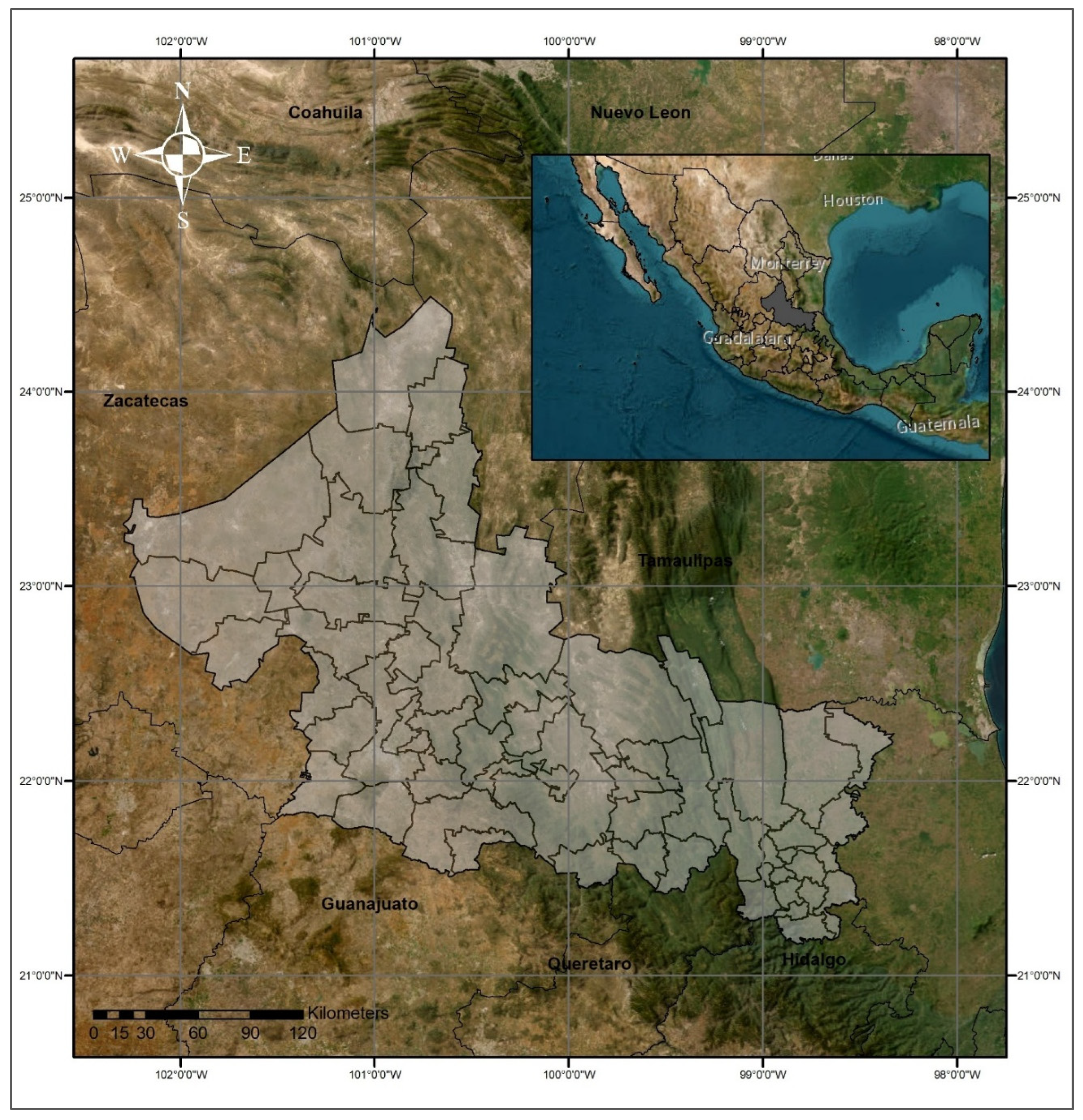
Figure 2.
Variables used and study area state context.
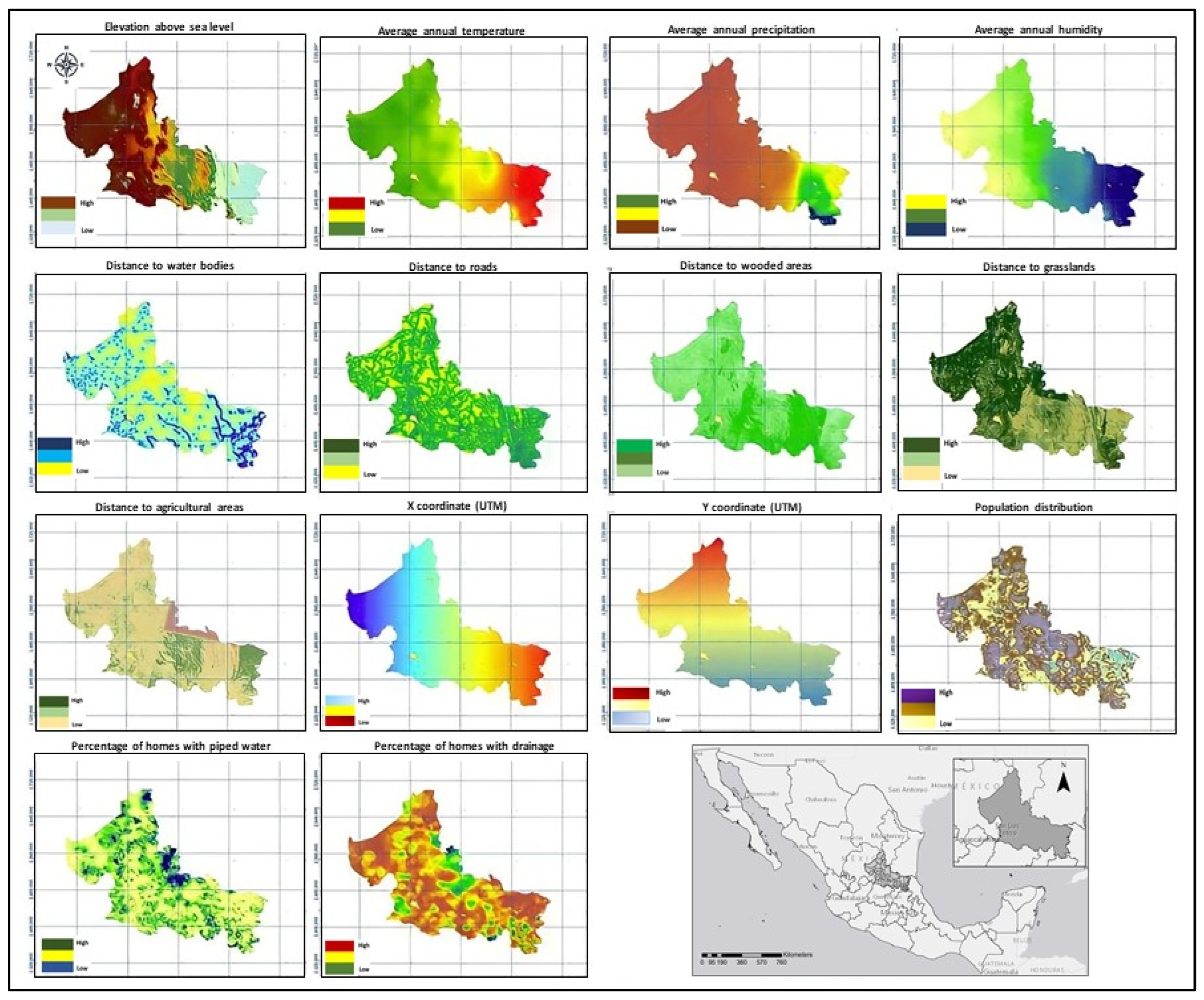
Figure 3.
Entity-relationship model of the dengue case database 2015–2020.
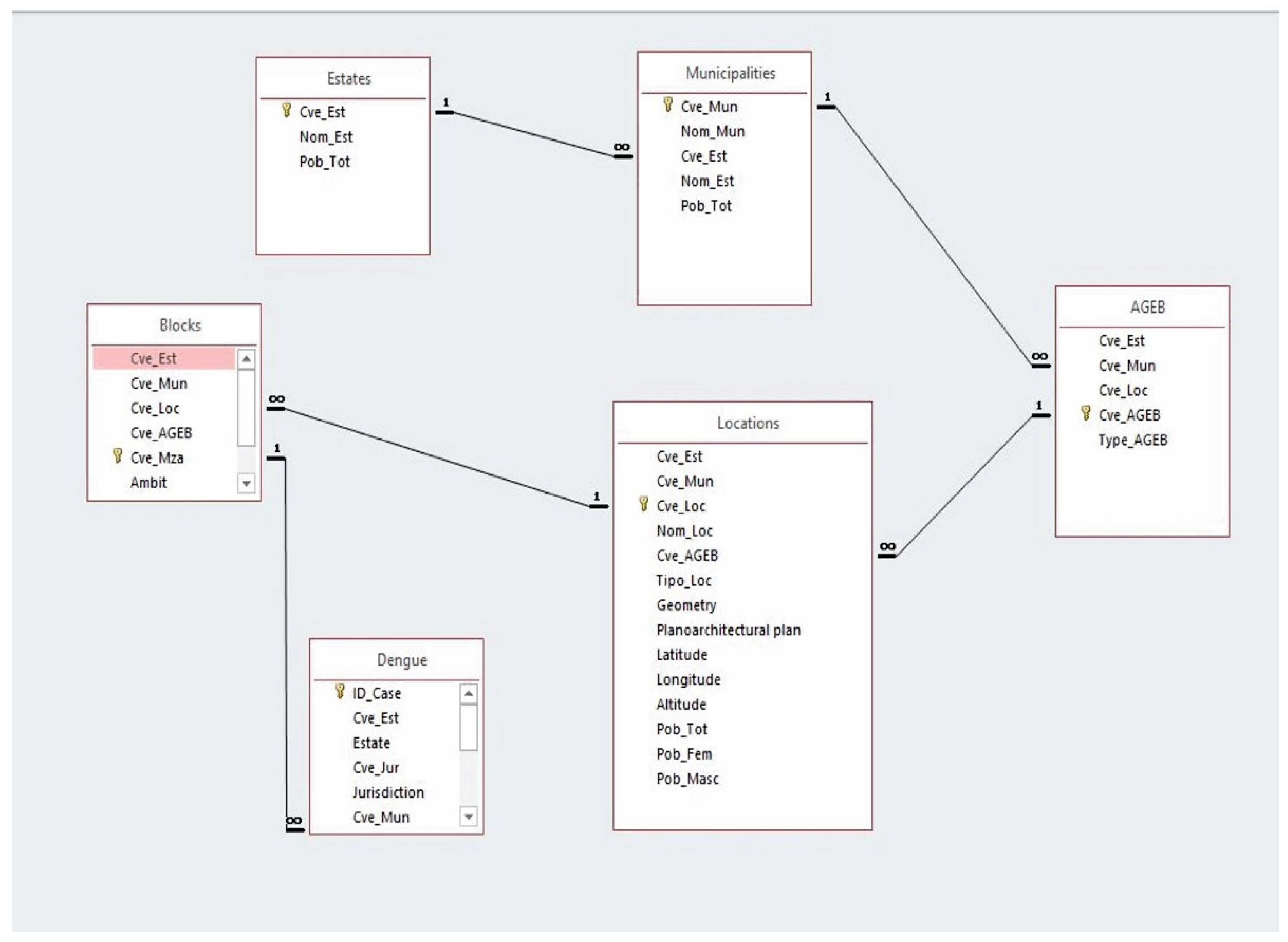
Figure 4.
Temporal evolution of dengue cases (2015–2020) in the Mexican state of San Luis Potosi.
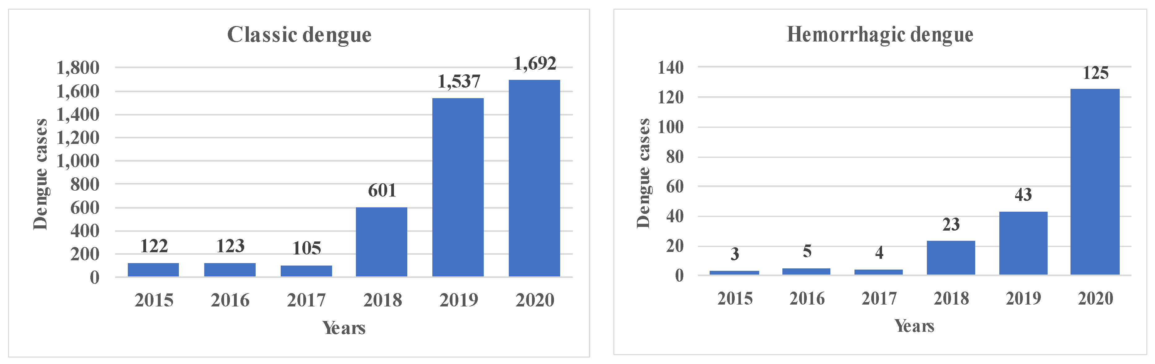

Table 1.
Variables used in the study.
| Variable | Type | Parameter | Year | Source | |
| Dependent variables | |||||
| Classic dengue fever | Health | Cases | 2015–2021 | [31] | |
| Hemorrhagic dengue fever | Health | Cases | 2015–2021 | ||
| Independent variables | |||||
| Elevation above sea level | Environmental | m | 2020 | [25,32] | |
| Average annual temperature | Environmental | °C | 2015–2020 | [16] | |
| Average annual rainfall | Environmental | mm | 2015–2020 | ||
| Average annual relative humidity | Environmental | % | 2015–2020 | [33] | |
| Distance to bodies of water | Proximity | m | 2015–2020 | [23] | |
| Distance to roads | Proximity | m | 2015–2020 | [25] | |
| Distance to wooded areas | Proximity | m | 2015–2020 | [23] | |
| Distance to grasslands | Proximity | m | 2015–2020 | [23] | |
| Distance to agricultural areas | Proximity | m | 2015–2020 | [23] | |
| XUTM | Location | m | 2020 | [25] | |
| YUTM | Location | m | 2020 | [25] | |
| Population | Social | Number of inhabitants | 2015–2020 | [25] | |
| Homes with piped water | Social | % | 2015–2020 | [25] | |
| Homes with drainage | Social | % | 2015–2020 | [28] | |
All variables included in the analysis were rasterized considering the extreme coordinates.
Table 2.
Comparison of the means of the variables used in the study.
| Variable** | Type of dengue | Median | Mean | ± SD | 95% CI | Minimum | Maximum | |
| Upper limit | Lower limit | |||||||
| Elevation above sea level (m)§* | No dengue | 0.0 | 610.7 | 785.1 | 583.4 | 638.1 | 0.0 | 2863.0 |
| Classic | 153.0 | 529.2 | 627.5 | 510.1 | 548.2 | 10.0 | 2106.0 | |
| Hemorrhagic | 201.0 | 692.7 | 725.7 | 592.3 | 793.1 | 19.0 | 1943.0 | |
| Average annual temperature (°C)£* | No dengue | 0.0 | 9.9 | 10.4 | 9.5 | 10.2 | 0.0 | 26.4 |
| Classic | 24.2 | 22.9 | 2.5 | 22.8 | 23.0 | 16.8 | 27.1 | |
| Hemorrhagic | 23.7 | 22.2 | 2.9 | 21.8 | 22.6 | 17.2 | 26.9 | |
| Average annual rainfall (mm)§¥ | No dengue | 0.0 | 296.6 | 436.8 | 281.3 | 311.8 | 0.0 | 2.3 |
| Classic | 1.5 | 1313.4 | 699.6 | 1292.2 | 1334.6 | 272.8 | 2393.5 | |
| Hemorrhagic | 1.5 | 1211.9 | 738.9 | 1109.6 | 1314.2 | 281.2 | 2265.6 | |
| Average annual relative humidity (%)£* | No dengue | 65.3 | 65.5 | 6.6 | 65.3 | 65.7 | 52.9 | 77.8 |
| Classic | 74.7 | 71.1 | 7.2 | 70.8 | 71.3 | 53.3 | 77.7 | |
| Hemorrhagic | 73.5 | 68.9 | 8.5 | 67.7 | 70.0 | 54.1 | 77.7 | |
| Distance to bodies of water (m)£ | No dengue | 1.5 | 35,535.3 | 4,3847.0 | 3,4006.4 | 37,064.2 | 0.0 | 204,812.6 |
| Classic | 1.5 | 2571.6 | 3042.8 | 2479.3 | 2663.9 | 0.0 | 25,497.1 | |
| Hemorrhagic | 1.9 | 2738.3 | 3457.5 | 2259.8 | 3216.7 | 0.0 | 19,440.4 | |
| Distance to roads (m)£ | No dengue | 4.9 | 29,161.4 | 4,3538.1 | 2,7643.3 | 3.0679.5 | 0.0 | 1.98009.7 |
| Classic | 90.0 | 170.4 | 218.9 | 163.8 | 177.1 | 0.0 | 2023.4 | |
| Hemorrhagic | 108.2 | 186.1 | 222.0 | 155.4 | 216.9 | 0.0 | 1171.5 | |
| Distance to grasslands (m)£* | No dengue | 1.9 | 27,688.6 | 43,314.5 | 26,178.3 | 29,198.9 | 0.0 | 197,347.0 |
| Classic | 60.0 | 127.2 | 269.9 | 119.1 | 135.4 | 0.0 | 2278.8 | |
| Hemorrhagic | 60.0 | 92.0 | 113.7 | 76.3 | 107.7 | 0.0 | 768.4 | |
| Distance to wooded areas (m)£* | No dengue | 3.3 | 28,392.1 | 4,3547.3 | 2,6873.6 | 2,9910.5 | 0.0 | 195,719.2 |
| Classic | 123.7 | 411.5 | 1,117.5 | 377.6 | 445.4 | 0.0 | 12,678.7 | |
| Hemorrhagic | 150.0 | 305.3 | 437.6 | 244.8 | 365.8 | 0.0 | 3390.9 | |
| Distance to agricultural areas£ | No dengue | 5.0 | 30,742.9 | 45,429.5 | 29,158.8 | 32,326.9 | 0.0 | 200,867.4 |
| Classic | 42.4 | 221.0 | 891.0 | 194.0 | 248.1 | 0.0 | 15,671.1 | |
| Hemorrhagic | 42.4 | 217.9 | 983.3 | 81.8 | 354.0 | 0.0 | 13,642.2 | |
| XUTM (m)£* | No dengue | 423,366.2 | 423,375.6 | 80,732.8 | 420,560.6 | 426,190.6 | 286,266.2 | 560,466.2 |
| Classic | 502,266.2 | 466,630.2 | 80,774.7 | 464,180.8 | 469,079.6 | 281,676.2 | 565,356.2 | |
| Hemorrhagic | 498,726.2 | 445,355.8 | 93,106.9 | 432,470.5 | 458,241.0 | 288,456.2 | 565,626.2 | |
| YUTM (m)£* | No dengue | 2,509,896.2 | 2,509,887.0 | 98,151.3 | 2,506,464.6 | 2,513,309.4 | 2,342,631.2 | 26,77,131.2 |
| Classic | 2,423,356.2 | 2,408,033.7 | 49,052.4 | 2,406,546.2 | 2,409,521.2 | 2,341,191.2 | 26,79,921.2 | |
| Hemorrhagic | 2,427,351.2 | 2,423,161.5 | 72,889.9 | 2,413,074.2 | 2,433,248.9 | 2,344,341.2 | 26,79,351.2 | |
| Population (n)£ | No dengue | 128.1 | 304.8 | 3161.0 | 194.6 | 415.0 | 2.7 | 93,466.2 |
| Classic | 620.8 | 7682.4 | 20,642.2 | 7056.5 | 8308.4 | 4.9 | 95,368.7 | |
| Hemorrhagic | 638.7 | 10,351.0 | 23,850.0 | 7050.3 | 13,651.6 | 7.3 | 92,941.6 | |
| Homes with piped water (%)£ | No dengue | 16.0 | 24.1 | 23.2 | 23.3 | 24.9 | 0.0 | 96.8 |
| Classic | 4.2 | 10.3 | 17.5 | 9.8 | 10.8 | 0.0 | 100.0 | |
| Hemorrhagic | 4.9 | 11.5 | 18.7 | 8.9 | 14.1 | 0.0 | 98.5 | |
| Homes with drainage (%)£ | No dengue | 10.0 | 16.3 | 17.1 | 15.7 | 16.9 | 0.0 | 83.6 |
| Classic | 8.0 | 12.5 | 13.8 | 12.1 | 13.0 | 0.0 | 90.1 | |
| Hemorrhagic | 9.1 | 13.5 | 14.2 | 11.5 | 15.4 | 0.0 | 63.9 | |
Significant difference in means (p < 0.05). Between: §No dengue and classic dengue fever; ¥No dengue and Dengue hemorrhagic fever; £No dengue, classic dengue fever and dengue hemorrhagic fever; *Classic dengue and dengue hemorrhagic fevers; **One-way analysis of variance.Bivariate logistic regression analysis.
Table 3.
Bivariate relationship between dengue cases and each independent variable.
| Variable | Classic dengue fever | Dengue hemorrhagic fever | ||
| Beta | p | Beta | p | |
| Elevation above sea level | -0.165E-03 | <0.001 | 0.130E-03 | 0.148 |
| Average temperature | 0.338 | <0.001 | 0.258 | <0.001 |
| Average annual rainfall | 0.268E-02 | <0.001 | 0.217E-02 | <0.001 |
| Average annual relative humidity | 0.104 | <0.001 | 0.719E-01 | <0.001 |
| Distance to bodies of water | -0.292E-03 | <0.001 | -0.318E-03 | <0.001 |
| Distance to roads | -0.405E-02 | <0.001 | -0.436E-02 | <0.001 |
| Distance to grasslands | -0.107E-02 | <0.001 | -0.180E-02 | <0.001 |
| Distance to wooded areas | -0.336E-03 | <0.001 | -1.888 | <0.001 |
| Distance to agricultural areas | -0.287E-03 | <0.001 | -0.529E-03 | <0.001 |
| XUTM | 0.634E-05 | <0.001 | 0.336E-05 | <0.001 |
| YUTM | -0.176E-04 | <0.001 | -0.192E-04 | <0.001 |
| Population | 0.767E-03 | <0.001 | 0.980E-04 | <0.001 |
| Homes with piped water | -0.348E-01 | <0.001 | -0.359E-01 | <0.001 |
| Homes with drainage | -0.159E-01 | <0.001 | -0.111E-01 | 0.021 |
Preliminary multivariate logistic regression analysis.
Table 4.
Preliminary multivariate logistic models to estimate vulnerability to dengue fever.
| Variable | Classic dengue fever | Dengue hemorrhagic fever | ||||
| Beta | p | Collinearity | Beta | p | Collinearity | |
| Elevation above sea level | -0.265E-02 | <0.001 | N | -0.297E-02 | <0.001 | S |
| Average temperature | 0.198 | <0.001 | N | 0.128 | 0.268 | N |
| Average annual rainfall | 0.911E-03 | <0.001 | N | 0.152E-02 | <0.001 | N |
| Average annual relative humidity | -0.131 | 0.001 | N | -0.369 | 0.001 | N |
| Distance to bodies of water | -0.413E-04 | 0.001 | S | -0.837E-04 | 0.008 | S |
| Distance to roads | -0.389E-02 | <0.001 | S | -0.377E-02 | <0.001 | S |
| Distance to grasslands | 0.975E-03 | <0.001 | S | -0.457E-04 | 0.937 | S |
| Distance to wooded areas | 0.143E-03 | 0.024 | S | -0.185E-03 | 0.218 | S |
| Distance to agricultural areas | -0.207E-04 | 0.518 | N | -0.971E-04 | 0.272 | S |
| XUTM | -0.274E-04 | <0.001 | S | 0.258E-05 | 0.746 | S |
| YUTM | -0.975E-05 | <0.001 | N | 0.379E-05 | 0.083 | S |
| Population | 0.209E-03 | <0.001 | N | 0.706E-04 | <0.001 | N |
| Homes with piped water | -0.676E-02 | 0.006 | N | -0.738E-02 | 0.192 | N |
| Homes with drainage | -0.111E-01 | 0.003 | N | -0.492E-02 | 0.560 | S |
| Constant | 39.639 | <0.001 | -- | 13.040 | 0.057 | -- |
Final multivariate logistic regression analysis.
Table 5.
Logistic models with standardized variables for estimating vulnerability to dengue fever.
| Variable | Classic dengue fever | Dengue hemorrhagic fever | ||
| Beta | p | Beta | p | |
| Elevation above sea level | -2.365 | <0.001 | - | - |
| Average annual temperature | 4.240 | <0.001 | 4.029 | 0.017 |
| Average annual rainfall | 0.646 | <0.001 | 1.936 | <0.001 |
| Annual relative humidity | -3.034 | <0.001 | -1.573 | 0.002 |
| Distance to agricultural areas | -3.861 | <0.001 | - | - |
| YUTM | -0.894 | <0.001 | - | |
| Population | 5.600 | <0.001 | 1.169 | <0.001 |
| Homes with piped water (%) | -0.152 | 0.001 | -0.384 | <0.001 |
| Homes with drainage (%) | -0.130 | 0.006 | - | - |
| Constant | -0.674 | 0.039 | -3.943 | <0.001 |
Table 6.
Percentage of the population vulnerable to dengue fever.
| Level of risk | Percentage of population | |
| Classic dengue fever | Dengue hemorrhagic fever | |
| Very low | 30.5 | 92.0 |
| Under | 6.1 | 4.2 |
| Medium | 8.0 | 1.5 |
| High | 9.2 | 1.4 |
| Very high | 46.3 | 0.9 |
Disclaimer/Publisher’s Note: The statements, opinions and data contained in all publications are solely those of the individual author(s) and contributor(s) and not of MDPI and/or the editor(s). MDPI and/or the editor(s) disclaim responsibility for any injury to people or property resulting from any ideas, methods, instructions or products referred to in the content. |
© 2025 by the authors. Licensee MDPI, Basel, Switzerland. This article is an open access article distributed under the terms and conditions of the Creative Commons Attribution (CC BY) license (http://creativecommons.org/licenses/by/4.0/).
Copyright: This open access article is published under a Creative Commons CC BY 4.0 license, which permit the free download, distribution, and reuse, provided that the author and preprint are cited in any reuse.


