
Submitted:
15 September 2025
Posted:
18 September 2025
You are already at the latest version
Abstract
The Lomb-Scargle method (LSM) constitutes a robust method for frequency and amplitude estimation in cases where data exhibit irregular or sparse sampling. Conventional spectral analysis techniques, such as the discrete Fourier transform (FT) and wavelet transform, rely on orthogonal mode decomposition and are therefore inherently constrained when applied to non-equidistant or fragmented datasets, leading to significant estimation biases. The classical LSM, originally formulated for univariate time series, provides a statistical estimator that does not assume a Fourier series representation. In this work, we extend LSM to multivariate datasets by redefining the shifting parameter τ to preserve the orthogonality of trigonometric basis functions in the Rn case. This generalization enables the simultaneous estimation of frequency, phase, and amplitude vectors while maintaining the statistical advantages of LSM, including consistency and noise robustness. As a demonstrative application, we analyze solar activity data, where sunspots serve as intrinsic markers of the solar dynamo process. These observations constitute a randomly sampled, two-dimensional binary dataset, whose characteristic frequencies are identified and compared with results from solar research. Additionally, the proposed method is applied to an ultrasound velocity profile measurement setup, yielding a three-dimensional velocity dataset with correlated missing values and significant temporal jitter. We derive confidence intervals for parameter estimation and conduct a comparative analysis with FT-based approaches.
Keywords:
multivariate data analysis
; spectroscopic
; uneven sampling
1. Introduction
In numerous signal processing applications, the characterization of a physical process via its power spectrum, or its amplitude and phase spectra, is of fundamental importance. Typically, the recorded signal is sampled at uniform intervals over a finite observation period and stored as discrete sampled data. Spectral analysis serves multiple purposes, including the identification of characteristic frequencies for process recognition, the selection or attenuation of specific spectral components, and the precise estimation of amplitude and phase at specified frequencies. Conventional approaches predominantly rely on the discrete Fourier transform (DFT) or its computationally efficient companion, the fast Fourier transform (FFT), both of which decompose the data into Fourier series coefficients, from which the power spectrum can be derived [1,2]. These transformations are inherently invertible, computationally efficient, and straightforward to implement. However, their applicability is constrained by the requirement of equidistant sampling, a limitation that poses challenges for data acquisition, in general. In practical applications, missing or corrupted data is often handled by substituting zero values, a common but problematic approach. In contrast to the intension, zero values provide some sort of information and do not mean “not aquired”. Subsequently, this procedure introduces a systematic error that leads to increased inaccuracies in frequency and amplitude estimation and ultimately affects the reliability of parameter estimation. While the DFT naturally extends to higher dimensions, facilitating applications such as image reconstruction in magnetic resonance imaging [3], image filtering [4], and higher-order spectral filtering in spatiotemporal domains [5], its performance deteriorates in the presence of non-uniform sampling. In ultrafast nuclear magnetic resonance (NMR) spectroscopy, non-uniform sampling enables substantial acceleration of chemical analysis [6,7], albeit at the cost of increased missing data, reduced sensitivity, and signal attenuation. These limitations are inherent to DFT-based and similar techniques, as they exhibit reduced accuracy when applied to incomplete datasets with data gaps [8]. Although alternative methods, such as the "non-uniform Fourier transform" [9,10,11], attempt to address these issues, they remain reliant on classical orthogonal mode decomposition (e. g., FFT, DFT, wavelet transform) and thus inherit systematic errors, as discussed in Section 2.2.
The application of techniques based on Fourier series to signals with non-equidistant sampling is difficult, since it usually requires zero padding (replacing missing values by zeros) on a grid and in the general case resampling or interpolation of the data to a regular grid [12,13]. The effect of a gap filling method is investigated extensively by Munteanu et al. [8]. The conclusion of the latter study is that without a corrective measure, errors such as amplitude minimization, which depends on the total gap density, cannot be avoided when FFT or DFT is applied. On the other hand, interpolation could be utilized to shift non-uniformly sampled data to a regular grid, so that the new interpolated data points are composed of the signal information and a projection of the accompanying noise. In the general case such distortions or noise are not band limited leading to biased estimates which consist of the local and aliased errors (noise, outliers, missing values, etc.) of the surrounding data.
Usually, astrophysical data is often affected by gaps, missing values and unevenly sampling. For example, when ground based radio telescopes are exploring areas in space there might exist time intervals in which the antenna is not pointing towards the object of interest due to the rotation of the Earth. The result is an incomplete data set. Non-uniform (random) sampling emerges for example if the irregular appearance of objects like Sunspots is measured as a binary quality depending on time and location. Section 5.3 provides a working example which analyzes frequencies and periods in latitude and time from the two dimensional data set of Sunspot observations. An other technical example for random sampling (with highly variable sampling frequency) is asynchronous data acquisition in large sensor networks, which are used in Smart Home, Industry 4.0 and automated driving, see Geneva et al. [14], Cadena et al. [15], Sudars [16]. Here the time series provide missing values and data gaps originating from time periods, in which strong noise prevents the measurement or simply the source of the signal to be measured is not in the range of the sensor.
The Lomb-Scargle method (LSM) was developed especially for ground based non-uniformly sampled one dimensional data, from which the amplitude spectrum is calculated [17,18]. The main advantage of this method is to directly estimate the spectrum without iterative optimization of trigonometric models as discussed in Section 2.1. A fast version for one dimensional signals is presented by Townsend [19] and Leroy [20].
An extension of LSM to two- or three-dimensional time series have not been presented yet. Especially for large multivariate data sets such a direct approach would be comparably faster than present iterative procedures as proposed in (Babu and Stoica [21], Chap. 9). The advantages of multivariate LSM will be demonstrated in Section 5 by means of a 3D Ultrasound flow profile measurement and the 2D analysis of Sunspot time series data.
In case of the analysis of flow profile measurements which are obtained in an experiment investigating the magnetorotational instability in liquid metals [22], such method would be highly desirable. Due to the complex experimental setup and the weak signal to noise ratio, the flow profile measurements contain several time intervals, in which distortions are dominant, see Seilmayer et al. [23]. These time intervals had to be rejected leading to a time series with invalid (missing) data points, from which the multivariate version of LSM is able to determine the parameters of the characteristic traveling wave.
In order to demonstrate the method and to motivate the basic idea of the multivariate version of LSM we compare it, in terms of necessary conditions and error (noise) behaviour, with the traditional orthogonal mode decomposition (OMD) with trigonometric basis functions, which is the essence of the classical Fourier transform. It will be shown that LSM fits better to the conditions of an arbitrary finite length of the sampling series in comparison to DFT, because LSM reduces the error in model parameter estimation. In contrast to the traditional approach, which was derived from a statistical point of view (see the appendix of Scargle [18]), the presented method is deduced from a technical point of view and focuses on its application. This leads to a slight change in the scaling of model parameters, which will be discussed in Section 4.2. However, the introduced procedure includes all benefits, like arbitrary sampling, fragmented data and a good noise rejection.
The starting point of this paper is the analysis of a continuous 1D signal which is composed of an arbitrary and finite set of individual frequency components . Without loss of generality, band limitation is assumed stating that there exists an upper maximum frequency with , which mimics an intrinsic low pass filter characteristic of the measurement device. Since the measurement time is finite, the value of s is only known in the time interval with and . The m-dimensional extension of this signal is . If such a continuous signal is sampled, the pair represents the measured 1D value and the corresponding instant in time whereas the pair represents a measured value and the m-dimensional location ( space/time) for the i-th sample (N is the number of samples). All the methods presented in this paper are implemented in a package written in R and published on CRAN [24]. The reader will find more elaborate examples in the package and in the supplementary material.
2. Mathematical Model and Comparison of OMD and LSM
In order to delineate the differences between trigonometric OMD and LSM, we start with the basic model of a periodic signal as a sum of signals of different frequencies with the corresponding amplitude and phase shift . The corresponding trigonometric model function
describes an infinite, stationary and steady process with the coefficients for the defined frequency and the identities as well as . Furthermore, the trigonometric model above consists of an arbitrary number of frequency components. If the given signal is described by the defined model from Equation (1) the model misfit is given by
Thus, the signal can now be described by inserting Equation (1) into Equation (2) and defining the misfit for each discrete frequency k with as follows:
The defined misfit originates form measurement uncertainties or parametric errors from , . In the general case can be any function or distribution. The challenge is to precisely determine the model parameters and for a given signal achieving minimal . This can be accomplished by one of the three methods described in the following sections: (i) Least-Square fit; (ii) orthogonal mode decomposition; (iii) Lomb-Scargle method (LSM).
2.1. Least Square Fit
The optimal fit is reached by least square fitting, resulting in a minimum , which was shown by Barning [25], Mathias et al. [26]. Since such procedures are iterative, the convergence of the algorithm might need a large number of function evaluations of Equation (3). Therefore, a direct version like LSM is preferable. It can be shown that LSM becomes equivalent to a least square fit of a sinusoidal model [17,25].
2.2. Trigonometric OMD
Generally, two functions are said to be orthogonal on the interval if the following condition holds, refer to Weisstein [27]:
By selecting and , the integration leads, by exploiting the identity , to , which is only zero, if This is true for any , if the length of the interval is a multiple of the period so that with . It is interesting to note that this interval can be shorted to one half of the period, if is zero. By exploiting this feature of the trigonometric functions, the individual model coefficients are calculated by multiplying the sine or the cosine to the measured data and integrating over all times as shown by (Cohen [1], Chap. 15):
For a measured signal, the integration can only be performed over the interval . It is obvious that an error is introduced, if . In order to investigate the properties of the finite integration, we will focus on the cosine term (Equation (5)), since the analysis of the sine term (Equation (6)) is similar. By setting the integral boundaries to the finite time interval and expressing the signal using Equation (3), the integral in Equation (5) can be written as
Using the identities and , Equation (7) becomes
The equation above indicates that the coefficient is effected by two errors (truncation) and (random) which might be nonzero for an arbitrary T. Thus, if both errors are neglected, the integral on the left hand side turns into an approximation of . Taking the consideration about the orthogonality described in Equation (4) into account, becomes only zero, if the integration time T is an integer multiple of . This means for the Fourier series that a given integration time T (observation window) defines the lowest allowed frequency . Furthermore, only multiples of this fundamental frequency with are allowed in the Fourier series because in this case.
The technical realization of OMD is called “quadrature demodulation”, which is the discrete version of equation (8) by replacing the integral over into a sum over the discrete sampled values and setting the truncation error to zero. For a time discrete signal with N samples and equidistant sampling with a constant sampling period , and , the parameter (corresponding to the frequency ) is approximated by
According to the previous considerations, the truncation error is larger than zero if the measurement range is not exactly a multiple of , as shown in Figure 1.
In this example a signal with a time period of is sampled with , . The total integration time is , being slightly longer than the period of the signal, which is indicated by the two additional sampling points after . The truncation error equals the gray shaded area.
Generally speaking, the sampling error in the discrete version can be estimated by
where , . The random error is modeled by the -quantile of the sampling error distribution related to the underlying process with its standard deviation (e. g. JCGM [28]). This estimates the confidence interval of and , respectively (see supplementary material for details).
The above considerations lead to following four statements, which are derived in detail in Section 2 of the supplementary material : (i) the maximum absolute value of the truncation error is bounded if , which is consistent with the experimental findings from Thompson and Tree [29]; (ii) is independent from the total number of samples N for a constant time T, which makes the OMD a non-consistent estimator for model parameters and ; (iii) by increasing the sample rate, the random error decreases by but scales with twice the standard deviation of noise distribution; (iv) DFT can be derived from Equation (10) by restricting to equidistant sampling with constant .
Concluding, the truncation error, which is an intrinsic feature of OMD, produces a systematic deviation from the true value depending on the difference between the sampling time interval and the corresponding period of the frequency of interest. In contrast to that, the random error diminishes with increasing sampling rate . A detailed discussion on this topic can be found in Thompson and Tree [29], Jerri [30], Shannon [31]. In case of multivariate and randomly sampled data the recent work of Al-Ani and Tarczynski [32] suggests two calculation schemes estimating the Fourier transform in the general case. The continuous time Fourier transform estimation (similar to Equation (9)) takes samples with arbitrary spacing as the general approach, in contrast to the secondly proposed discrete time Fourier transform ( and ) estimation scheme. Here the data is projected onto a regular grid, which now may provide locations of missing data. Both schemes consider the sampling pattern and its power spectrum distribution function . However, even for such sophisticated methods, the main conceptual drawbacks (see points (i) and (ii)) remain, which motivates the subsequent Lomb-Scargle method as non OMD method and its extension to multivariate data.
2.3. Lomb Scargle Method
As described in the previous section, the disadvantage of OMD is that cosine and sine are not orthogonal on arbitrary intervals. By introducing an additional parameter into Equation (4) it will be shown that
holds for arbitrary intervals . By utilizing the trigonometric identities, and , to remove the differences in the arguments the integral can be transformed to
If this integral has to be zero, the following condition has to hold
which can be transformed to
Therefore, from Equation (12) the parameter verifying Equation (11) may be found. In case of equidistant sampling, the value of can be directly calculated from the integration boundaries by:
Based on this general consideration and in order to remove the truncation error, for each frequency the time shifting parameter was introduced by Lomb and Scargle [17,18] into the model given in Equation (1) so
The parameter can be calculated by
similar to Equation (12). For the time discrete version the integrals transform into a sum resulting in
The parameters can be determined beginning with Equation (7) but by factorising them by , instead of expanding to as done for Equation (8). In the following, the method is delineated for the discrete set since it is applied to sampled data. This data is multiplied by resulting in the next equation for a single frequency :
where . The sum of the terms vanishes because of the proper selection of according to Equation (15). The sum of the terms describes a modulated noise distribution function. The value of the parameters can be directly obtained by dividing by . This gives
The residual error term on the right hand side, , consists of a random distributed part divided by a sum over the square of the cosine. In contrast to OMD, the estimation error of the parameter only depends on noise and is independent from the realization of sampling.
The next step is to determine in terms of a confidence interval with respect to -quantile of the sampling error distribution , as it was done for OMD in Equation (10). Given a normal distributed error function with zero expectation value and a standard deviation independent from time (), the error can be factorized (Parzen [33], Theorem 4A, p. 90), leading to
estimating the most probable limits of . In the above equation neither depend on the frequency nor the shifting parameter and is defined as
The final parameter estimation gives
where the confidence interval converges to zero by increasing the number of samples N, for a fixed time interval. This property qualifies LSM to be a consistent estimator in amplitude and phase [26]. In addition, the confidence interval for the LSM is smaller than the value given in Equation (10) for the OMD (this also occurs for the confidence interval of the parameters , ). We notice that the definition of given in Equation (18) is slightly different from the original definition given by Lomb [17] but both definitions converge for large N (see supplementary material).
The confidence interval for the amplitude, , can be deduced by propagating the error :
In a similar way, the confidence interval for the phase can be defined by
It is interesting to note that the confidence interval for the phase decreases for increasing amplitude.
3. Spectrum from the Lomb-Scargle Method
In order to determine the spectrum with LSM, we assume the recorded signal is described by many frequencies. The most significant frequency is then represented by a peak in the frequency spectrum of a certain width and height. The width is determined by the frequency resolution which equals . From this point of view the precision of a frequency estimation changes only with observation length T and seams to be independent from the number of samples N and signal quality.
The quality is measured by a signal-to-noise ratio like expression
with counting the significant amplitudes. In Equation (19) is the fitted model, is the uncertainty per sample, with , and is the noise per sample. Following VanderPlas [34], we apply Bayesian statistics and assume that every peak is Gaussian shaped, i. e. . It follows that a significant peak appears at , in a way that is valid. Here, is related to the power spectral density . The frequency uncertainty (or standard deviation) is then given by
so that a significant peak is located in the interval . This approach suggests that increasing the number of samples in a fixed interval T enhances the precision of by reducing However, if the original signal contains two frequencies with a distance in the range of , it cannot be excluded even for LSM that these peaks merge together in one single peak with small according to Kovács [35].
Concluding the properties of LSM: (i) there is no truncation error ; (ii) LSM provides a better noise rejection compared to OMD, ; (iii) the explicit sampling pattern is not of interest to work with LSM.
4. The Multivariate Lomb-Scargle Method
A signal S depending of m-independent variables represents a function with the input vector described by . The model function for multivariate LSM is gained by replacing the scalar arguments of cosine and sine of the univariate model function of Equation (13) by vectors, resulting in
In this case, the shifting parameter is a vector and in principle, hard to calculate. However, if the argument of the cosine is expanded, it is obvious that the scalar product does not depend on time and thus, the cosine argument can be written as with . The determination of is similar as for shown in Equation (14), but with some differences in the equations since the phase, instead of the time coordinate, is shifted now. This determination is described in the following.
4.1. Derivation of the Shifting Parameter
This section shows that shifting the phase, instead of time, does not affect the Lomb-Scargle algorithm. The derivation of the shifting parameter for the multivariate case is delineated for the time discrete signal Starting with the orthogonality condition
and applying the trigonometric identities to remove the differences in the arguments:
By using the defined abbreviations and rearranging the summation (the terms and do not depend on n), the following equation is easily deduced:
The fraction on both sides can be further simplified by applying , , and the definition of the tangent. This results in
Notice that in comparison with one dimensional LSM, the frequency is missing on the left side in Equation (20).
4.2. Parameter Estimation
Similar to the procedure for the LSM for a discrete signal in one dimension (see Equation (16)), a discrete multivariate signal with N samples is multiplied by resulting in
The determination of the parameter , and its confidence interval , are similar to the one-dimensional case shown in Equation (18):
The parameter , and its confidence interval , are calculated analogously:
We recall that the -quantile of the sampling error distribution (with standard deviation ) has been used to model the random error. The power spectral density, as well as the false alarm probability, are calculated in the same way compared to the one dimensional LSM method (see supplementary material).
An implementation of the multivariate Lomb-Scargle method is available, in the spectral (R) package published on CRAN [24], to give the user access to a multi-dimensional analysis with an easy to use interface.
5. Application
The selected applications are ordered by increasing complexity of the sampling, and the data itself. First, a regular grid with missing values for a synthetic test data is considered. Second, Ultrasound Doppler Velocimetry (UDV) measurement data, which contains jitter and missing values is analized. Finally, a quite general data scenario given by an astrophysical 2D set of Sunspots, which appear freely in time and space, is investigated.
5.1. Synthetic Test Data
We start with a simple test case, where the input signal is a simple two dimensional plain wave , with and representing the dimensionless frequencies, specifically selected in such a way that , with and . The 2D sampling of is performed with . With respect to the chosen frequencies and it becomes evident, that both frequencies do not fit to the data range by an integer fraction. Data gaps are introduced by removing randomly distributed and uncorrelated grid points covering 60% of the total data set. Figure 2(a) shows the nonuniform distributed input data. Gray areas indicate missing values (non available numbers “”). As LSM requires an appropriate input vector of frequencies we choose for both variables with a resolution of .
The corresponding power spectral density (PSD) from the LSM (see supplementary material), shown in Figure 2(b), displays the maxima at the 1st and 3rd quadrant, which represents a wave traveling upwards. The figure illustrates that even with a huge amount of missing data, it is possible to properly detect the periodic signal. In the present case, the value of indicates a perfect fit to the corresponding sinusoidal model. For comparison, Figure 2(c) depicts the standardized PSD
calculated from a discrete Fourier transform DFT symbolized by the operator . Here, missing values () are handled by zero padding which means that the introduced gaps are filled with zero. Since the DFT represents a conservative transformation (mapping) into the spectral domain, zero padding leads to a significant reduction of the average signal energy. A proper rescaling to the number of zeros (missing values) is required, to ensure approximated amplitude estimations. Zero padding always changes the character of the input signal, in a way that the corresponding DFT threats the zeros as if they where part of the original signal. The resulting PSD becomes then finally different from the original one. Since the signal frequencies do not fit into an integer spaced scheme of the data range, the DFT suffers from its drawbacks, as is briefly discussed in Section 2.2. The effect of leakage and misfit of frequencies can be recognized in Figure 2(c), in terms of a rather coarse resolution and a lower PSD value.
5.2. 3D UDV Flow Measurement
The second example is taken from previous experimental flow measurements [22] devoted to investigate the azimuthal magneto-rotational instability AMRI. The experiment consists of a cylindrical annulus containing a liquid metal between the inner and the outer wall. The inner wall rotates at a frequency whereas the outer wall rotates at a frequency . The flow is driven by the shear, since . Two ultrasound sensors mounted at the outer cylinder, on opposite side of each other and at the same radius, measure the axial velocity component along the line of sight parallel to the rotation axis of the cylinder. Additionally, the liquid metal flow is exposed to a magnetic field (r is the radial coordinate), originated from a current on the axis of the cylinder. A typical time series of the axial velocity (along the measuring line) is displayed in Figure 3. The existence of periodic patterns (large blue inclined stripes) in this figure indicates a travelling wave propagating in the fluid. In cylindrical geometry, a travelling wave is described in terms of the drift frequency , the vertical wave numbers k, and the azimuthal wave numbers m. A close look to Figure 3 evidences that this wave is not axially symmetric, and that the leading azimuthal wave number is . This is indeed proven in the following with the LSM analysis.
The measured time series for depends on time , depth and the angular positions of the sensors and , where the subscript n indicates the sampling. The azimuthal angles depend on time, since the sensors are attached to the outer wall. This induces the mapping , where is meant to be one out of the set of two sensors at each sampling instance. Finally the measured velocity component is a mapping , which fits perfectly to the proposed multivariate LSM.
Figure 4 illustrates the result of the LSM decomposition into several azimuthal m-modes with the corresponding amplitudes. The mode contains a stationary structure, at a frequency , which originates from sensor miss-alignments and (thermal) side effects in the flow. The minor non-stationary components, here the two point-symmetric peaks, originate from cross-talk (or alias projections, see labels on Figure 4) of the mode. This is mainly for two reasons: First, because the sensors behave not exactly identical (e. g. misalignment or different sensitivity) and therefore respond slightly different to the same flow signal. This means that one of the sensors projects a little bit more energy into the data than the other, which leads to a “leakage”-effect and a weak signal in mode. Second, the rotation of the sensors acts like an additional sampling frequency . In consequence, the spectrum of this regular sampling function folds with the spectrum of the observed process, leading to alias images (copies) of the original process spectrum into other frequency ranges (i. e. m’s). In the present multivariate analysis, these alias structures exhibit point symmetry in panel, indicating corresponding traveling waves. It is evident that these aliases originate as a systematic error from the LSM method and, due to their symmetry, effectively cancel each other out. One could also argue, that multivariate LSM enables a robust identification of alias amplitudes, which do not belong to the observed process.
The AMRI wave itself is located in the panel, with a characteristic frequency in time (f) and in the vertical direction (k). Here, two components can be identified: the dominant wave at and and a minor counterpart at and . The signals observed in the and panels might be due to aliases, because of the rotation of the inner cylinder at a frequency .
The advantage of “high” dimensional spectral decomposition is the improved noise rejection. With respect to the raw data, given in Figure 3, it is obvious that high frequency noise is present in the data. Depending on the exact distribution of this noise, its energies spread over a certain range of frequencies. If we would select a representative depth and angle so that , the velocity only depends on time. In the subsequent one dimensional analysis the noise would accumulate along the single frequency ordinate probably hiding the signal of interest. Taking the higher order analysis distributes the noise energies over multiple domain variables. For the present example, this means that the distortions are projected into higher frequencies f, higher m’s and larger k’s. Since the signal of interest remains in the same spectral corridor, its signal amplitude becomes more clear, because of the “reduced” local noise.
5.3. Analyzing 2D s Unspot Data
Since the beginning of the 17th century systematic visual observations of Sunspots are available. This allows to investigate dynamic processes taking place in the Sun. The appearance of Sunspots on the Sun’s surface depends on the level of solar activity, and therefore it renders some fundamental features of the underlying solar dynamo, such as the solar cycle. Since the beginning of the 1820’s observational data is available, in terms of a two dimensional time series displayed in Figure 5. The data exhibits a periodic wing-like pattern essentially symmetric with respect to the Sun’s equator, the Sunspot butterfly diagram. This diagram summarizes the individual Sunspot groups appearing, at a certain time and latitude on the Sun, for the past 190 years. Additionally, Figure 5 depicts the assigned field polarity order indicated by the Sunspot color (gray or black). Given a year Y and a mean latitude L (degrees), the field polarity gives the arrangement of leading North/South polarity of a Sunspot group. This polarity is changing approximately each 11 yrs, which is called Schwabe’s cycle. The full period of is called the Hale cycle. The segmentation of Figure 5 is obtained following suggestions from Leussu et al. [36], but with some simplifications leading only to minor miss-assignments for individual Sunspot groups.
The Sunspot data is taken as-is from Leussu et al. [37], which originates from several sources with different qualities, i. e. the Royal Greenwich Observatory – USAF/NOAA(SOON)1[38,39], Schwabe2[40] and Spoerer3[43] data sets. A detailed discussion of the data collection is given by Leussu et al. [36], Leussu et al. [37] and the referenced literature.
In this section, the LSM spectral decomposition from this unevenly sampled binary data set is obtained, in order to identify typical periods. In contrast to the two examples analysed in Section 5.1 and Section 5.2, the Sunspot data set consists of real arbitrary sampling in both, time and space, providing the most general scenario input data for the LSM. The starting point for the subsequent analysis is the simplified segmentation of the butterfly diagram reassigning the field polarity. The segmentation takes place by optimizing the distance d (in the -plane) between each Sunspot and the segmentation line
which is a piece wise linear function with intersection point . The individual slopes, with , are assigned on the northern and southern hemispheres, respectively. The final segmentation of Figure 5 consist of 18 individual cycles subdivided by a > - shaped separation area.
The LSM spectral decomposition is based on the definition of a two dimensional wave model
where P is given by the assigned patch polarity. To show the advantage and robustness of the LSM the raw data is employed without any further preprocessing. The selected frequencies are given on a rectangular grid with inverse distance so that the periods are distributed uniformly alongside the consecutive counter n. Furthermore, the frequency resolution close to is selected finer to better resolve this region.
Figure 6 gives the resulting LSM spectral decomposition in a reciprocal log-scale plot to analyse the different periods. Each of the selected peaks (numbered black dots) provides a FAP value of , meaning that these periods are significantly different from noise level. Each of these points originate from a local frequency refinement to achieve the local maximum amplitude. The binary order information induced by the Sunspots, introduces higher harmonics into the spectrum, which do also appear with a significantly low FAP value.
Figure 6 provides good agreement between the peaks found and the common known periods. Table 1 summarizes the major outcome in comparison with literature. For example the Hale cycle varies from (Usoskin [44]) which is identified by the two main peaks. Since the solar cycle is modulated, refer to Hathaway [45], it is natural that a broad spectrum with many harmonics becomes present. These subsequent patterns are related to a set of local maxima mainly collapsing on a horizontal line at , indicating that the complex structure of the individual wing-shapes of the butterfly diagram with different widths, heights and orientation, corresponds to a main period . Next to that we can identify typical periods which are related to the Gleissberg process (see Table 1) or the short periods in the range of , which are consistent with the data provided by Prestes et al. [46], Kane [47] and partly with Deng et al. [48].
The latitudinal dimension of the spectrum spreads the peaks vertically which is a great advantage compared to a purely 1D analysis, where all signal would be projected on the line. In addition, complex patterns such as lines of constant phase velocities (dashed curve of Figure 6) may be used to analyse modulations of the dynamics of the Sunspot motion.
6. Conclusions
In the present work a multidimensional extension of the Lomb-Scargle method is developed. The key aspect is the redefinition of phase argument to . We suggest using a modified shifting parameter in contrast to the traditional approach which shifts the ordinate instead of the phase. This enables multivariate modeling with one single scalar value for all independent variables as there is always a shifting parameter for which vanishes on any interval .
With respect to the evaluation of measurement results, the noise rejection and confidence intervals ( and ) of model parameters and are delineated. To emphasize the advantages of the LSM the traditional Fourier mode decomposition is compared. It turned out that the systematic error does not vanish for FT based methods with increasing number of samples on a fixed interval T, which finally lead to the common leakage effect. Here the signal amplitudes are distributed on an area of neighboring spectral components, i. e. individual bins or pixels. We conclude that the standard orthogonal mode related procedures do not represent a consistent estimator for model parameters and . Whereas the introduction of in LSM leads to a consistent estimator with even for higher dimensions. Finally, it was shown that LSM converges to the true model parameters with increasing number of samples and provides a better noise rejection () as well.
The examples from Section 5 underline the strengths of the developed procedure in a consecutive way. First the application on ideal two dimensional test data shows the ability to analyze fragmented time series. Here the sampling remains regular meaning with , but with as an incomplete set of locations to describe missing values. A second quasi similar situation is given in the experimental data set of UDV measurements, expect a certain jitter. The dimensionality in this example was extended to to decompose the wave parameters in frequency f, symmetry m and spatial frequency k.
As the third analysis, the Sunspot data sets represent the most general case of non-evenly sampling. Taking only the time series of positions into account, LSM is able calculate the spectrum on a individual frequency grid pronouncing the low frequencies close to zero. The assignment of to each data point is a minor modification so the data can be assumed as binary raw data. The spectral decomposition with LSM shows the characteristic footprint of waves and its dynamics present in the butterfly diagram. The time frequency spectrum itself provides the commonly known frequencies, i. e. Hale-Cycle or Gleissberg process. The second frequency provides information about the minor peaks which are spread out into the latitudinal domain. Moreover, from these values the Sunspot drift motion may be calculated using a characteristic v-line with its side bands.
Acknowledgments
The authors like to thank Rainer Arlt from Astrophysical Institute Potsdam providing the Sunspot data and Andre Gieseke from HZDR for many fruitful discussions. F. Garcia kindly acknowledges the Serra Húnter and SGR (2021-SGR-01045) programs of the Generalitat de Catalunya (Spain).
References
- Cohen, L. Time-Frequency Analysis; Prentice Hall signal processing series; Prentice Hall PTR: Englewood Cliffs, N.J, 1995. [Google Scholar]
- Oppenheim. Discrete-Time Signal Processing, 2nd ed.; Prentice Hall, 1999.
- Haacke, E. Magnetic Resonance Imaging: Physical Principles And Sequence Design; John Wiley and Sons, 1999.
- Gonzalez, R.C.; Woods, R.E. Digital Image Processing, 3rd ed.; Prentice Hall, 2008.
- James, J. A Student’s Guide to Fourier Transforms: with Applications in Physics And Engeneering, 3rd ed.; Cambridge University Press, 2011.
- Frydman, L.; Lupulescu, A.; Scherf, T. Principles and Features of Single-Scan Two-Dimensional NMR Spectroscopy. Journal of the American Chemical Society 2003, 125, 9204–9217. [Google Scholar] [CrossRef]
- Giraudeau, P.; Frydman, L. Ultrafast 2D NMR: An Emerging Tool in Analytical Spectroscopy. Annual Review of Analytical Chemistry 2014, 7, 129–161. [Google Scholar] [CrossRef]
- Munteanu, C.; Negrea, C.; Echim, M.; Mursula, K. Effect of data gaps: comparison of different spectral analysis methods. Annales Geophysicae 2016, 34, 437–449. [Google Scholar] [CrossRef]
- Fessler, J.A. Iterative Tomographic Image Reconstruction Using Nonuniform Fast Fourier Transforms 2002. p. 11.
- Fessler, J.; Sutton, B. Nonuniform fast fourier transforms using min-max interpolation. IEEE Transactions on Signal Processing 2003, 51, 560–574. [Google Scholar] [CrossRef]
- Liu, Q.; Nguyen, N. An accurate algorithm for nonuniform fast Fourier transforms (NUFFT’s). IEEE Microwave and Guided Wave Letters 1998, 8, 18–20. [Google Scholar] [CrossRef]
- Press, W.H.; Rybicki, G.B. Fast Algorithms for Spectral Analysis of Unevenly Sampled Data. The Astrophysical Journal 1989, 338, 277–280. [Google Scholar] [CrossRef]
- Greengard, L.; Lee, J.Y. Accelerating the Nonuniform Fast Fourier Transform. SIAM Review 2004, 46, 443–454. [Google Scholar] [CrossRef]
- Geneva, P.; Eckenhoff, K.; Huang, G. Asynchronous Multi-Sensor Fusion for 3D Mapping And Localization. In Proceedings of the 2018 IEEE International Conference on Robotics and Automation (ICRA), Brisbane, QLD; 2018; pp. 1–6. [Google Scholar] [CrossRef]
- Cadena, C.; Carlone, L.; Carrillo, H.; Latif, Y.; Scaramuzza, D.; Neira, J.; Reid, I.; Leonard, J.J. Past, Present, and Future of Simultaneous Localization and Mapping: Toward the Robust-Perception Age. IEEE Transactions on Robotics 2016, 32, 1309–1332. [Google Scholar] [CrossRef]
- Sudars, K. Data acquisition based on nonuniform sampling: Achievable advantages and involved problems. Automatic Control and Computer Sciences 2010, 44, 199–207. [Google Scholar] [CrossRef]
- Lomb, N.R. Least-Squares Frequency Analysis of Unequally Spaced Data. Astrophysics and Space Science 1976, 39, 447–462. [Google Scholar] [CrossRef]
- Scargle, J.D. Studies in Astronomical Time Series Analysis. II - Statistical Aspects of Spectral Analysis of Unevenly Spaced Data. The Astrophysical Journal 1982, 263, 835–853. [Google Scholar] [CrossRef]
- Townsend, R.H.D. Fast Calculation of the Lomb-Scargle Periodogram Using Graphics Processing Units. The Astrophysical Journal Supplement Series 2010, 191, 247. [Google Scholar] [CrossRef]
- Leroy, B. Fast calculation of the Lomb-Scargle periodogram using nonequispaced fast Fourier transforms. Astronomy & Astrophysics 2012, 545, A50. [Google Scholar] [CrossRef]
- Babu, P.; Stoica, P. Spectral analysis of nonuniformly sampled data – a review. Digital Signal Processing 2010, 20, 359–378. [Google Scholar] [CrossRef]
- Seilmayer, M.; Galindo, V.; Gerbeth, G.; Gundrum, T.; Stefani, F.; Gellert, M.; Rüdiger, G.; Schultz, M.; Hollerbach, R. Experimental Evidence for Nonaxisymmetric Magnetorotational Instability in a Rotating Liquid Metal Exposed to an Azimuthal Magnetic Field. Physical Review Letters 2014, 113, 024505. [Google Scholar] [CrossRef]
- Seilmayer, M.; Gundrum, T.; Stefani, F. Noise Reduction of Ultrasonic Doppler Velocimetry in Liquid Metal Experiments with High Magnetic Fields. Flow measurement and instrumentation 2016, 48, 74–80. [Google Scholar] [CrossRef]
- Seilmayer, M. Common Methods of Spectral Data Analysis, 2019.
- Barning, F.J.M. The Numerical Analysis of the Light-Curve of 12 Lacertae. Bulletin of the Astronomical Institutes of the Netherlands 1963, 17, 22. [Google Scholar]
- Mathias, A.; Grond, F.; Guardans, R.; Seese, D.; Canela, M.; Diebner, H.H.; Baiocchi, G. Algorithms for Spectral Analysis of Irregularly Sampled Time Series. Journal of Statistical Software 2004, 11, 1–30. [Google Scholar] [CrossRef]
- Weisstein, E.W. Orthogonal Functions, 2019.
- JCGM. Evaluation of measurement data – Guide to the expression of uncertainty in measurement, 2008.
- Thompson, J.K.; Tree, D.R. Leakage error in Fast Fourier analysis. Journal of Sound and Vibration 1980, 71, 531–544. [Google Scholar] [CrossRef]
- Jerri, A.J. The Shannon Sampling Theorem—Its Various Extensions And Applications: A Tutorial Review. Proceedings of the IEEE 1977, 65, 1565–1596. [Google Scholar] [CrossRef]
- Shannon, C.E. Communication in the Presence of Noise. Proceedings of the IRE 1949, 37, 10–21. [Google Scholar] [CrossRef]
- Al-Ani, M.; Tarczynski, A. Evaluation of Fourier transform estimation schemes of multidimensional signals using random sampling. Signal Processing 2012, 92, 2484–2496. [Google Scholar] [CrossRef]
- Parzen, E. Stochastic Processes; Holden Day Series in Probability and Statistics; Holden-Day: San Francisco, 1962. [Google Scholar]
- VanderPlas, J.T. Understanding the Lomb-Scargle Periodogram. The Astrophysical Journal 2017, 236. [Google Scholar] [CrossRef]
- Kovács, G. Frequency Shift in Fourier Analysis. Astrophysics and Space Science 1981, 78, 175–188. [Google Scholar] [CrossRef]
- Leussu, R.; Usoskin, I.G.; Arlt, R.; Mursula, K. Properties of sunspot cycles and hemispheric wings since the 19th century. Astronomy & Astrophysics 2016, 592, A160. [Google Scholar] [CrossRef]
- Leussu, R.; Usoskin, I.G.; Pavai, V.S.; Diercke, A.; Arlt, R.; Denker, C.; Mursula, K. Wings of the butterfly: Sunspot groups for 1826–2015. Astronomy & Astrophysics 2017, 599, A131. [Google Scholar] [CrossRef]
- Clette, F.; Svalgaard, L.; Vaquero, J.M.; Cliver, E.W. Revisiting the Sunspot Number. A 400-Year Perspective on the Solar Cycle. Space Science Reviews 2014, 186, 35–103. [Google Scholar] [CrossRef]
- Willis, D.M.; Wild, M.N.; Warburton, J.S. Re-examination of the Daily Number of Sunspot Groups for the Royal Observatory, Greenwich (1874 – 1885). Solar Physics 2016, 291, 2519–2552. [Google Scholar] [CrossRef]
- Arlt, R.; Leussu, R.; Giese, N.; Mursula, K.; Usoskin, I.G. Sunspot positions and sizes for 1825-1867 from the observations by Samuel Heinrich Schwabe. Monthly Notices of the Royal Astronomical Society 2013, 433, 3165–3172. [Google Scholar] [CrossRef]
- Spoerer, G. Mémoires et observations. Sur les différences que présentent l’hémisphère nord et l’hémisphère sud du soleil. Bulletin Astronomique, Serie I 1889, 6, 60–63. [Google Scholar] [CrossRef]
- Spoerer, F.W.G.; Maunder, E.W. Prof. Spoerer’s researches on Sun-spots. Monthly Notices of the Royal Astronomical Society 1890, 50, 251. [Google Scholar] [CrossRef]
- Diercke, A.; Arlt, R.; Denker, C. Digitization of sunspot drawings by Spörer made in 1861-1894: Digitization of sunspot drawings by Spörer made in 1861-1894. Astronomische Nachrichten 2015, 336, 53–62. [Google Scholar] [CrossRef]
- Usoskin, I.G. A history of solar activity over millennia. Living Reviews in Solar Physics 2017, 14, 3. [Google Scholar] [CrossRef]
- Hathaway, D.H. The Solar Cycle. Living Reviews in Solar Physics 2015, 12, 4. [Google Scholar] [CrossRef]
- Prestes, A.; Rigozo, N.R.; Echer, E.; Vieira, L.E.A. Spectral analysis of sunspot number and geomagnetic indices (1868–2001). Journal of Atmospheric and Solar-Terrestrial Physics 2006, 68, 182–190. [Google Scholar] [CrossRef]
- Kane, R.P. Quasi-biennial and quasi-triennial oscillations in geomagnetic activity indices. Annales Geophysicae 1997, 15, 1581–1594. [Google Scholar] [CrossRef]
- Deng, H.; Mei, Y.; Wang, F. Periodic variation and phase analysis of grouped solar flare with sunspot activity. Research in Astronomy and Astrophysics 2020, 20, 022. [Google Scholar] [CrossRef]
- McCracken, K.; Beer, J.; Steinhilber, F.; Abreu, J. The Heliosphere in Time. Space Science Reviews 2013, 176, 59–71. [Google Scholar] [CrossRef]
- Ogurtsov, M.G.; Nagovitsyn, Y.A.; Kocharov, G.E.; Jungner, H. LONG-PERIOD CYCLES OF THE SUN’S ACTIVITY RECORDED IN DIRECT SOLAR DATA AND PROXIES 2002. p. 24.
- Kolotkov, D.Y.; Broomhall, A.M.; Nakariakov, V.M. Hilbert–Huang transform analysis of periodicities in the last two solar activity cycles. Monthly Notices of the Royal Astronomical Society 2015, 451, 4360–4367. [Google Scholar] [CrossRef]
| 1 |
Available at
http://solarscience.msfc.nasa.gov/greenwch.shtml
|
| 2 |
Available at
http://www.aip.de/Members/rarlt/sunspots/schwabe
|
| 3 |
Figure 1.
Example of the truncation error of a signal with the time period of , which is generated by the last two samples and the value is indicated by the gray shaded area.
Figure 1.
Example of the truncation error of a signal with the time period of , which is generated by the last two samples and the value is indicated by the gray shaded area.
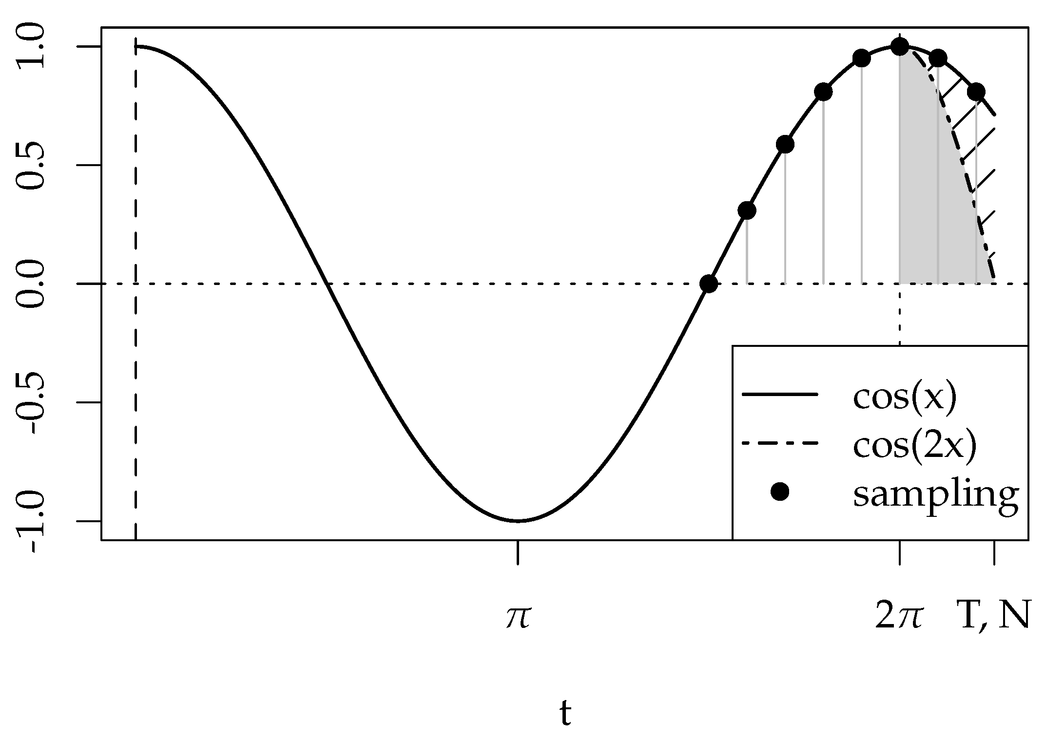
Figure 2.
Comparison of the PSD calculated with the LSM and with the DFT approach for a two-dimensional input data with missing values. (a) Sampled data , for with sampling increment , and and . Gray areas represent missing values. (b) PSD calculated with the LSM and (c) PSD calculated with DFT. Notice that the truncation error and the sparse resolution leads to a rough approximation of the frequency, and to a reduced amplitude (by 50%), in the PSD calculated by DFT.
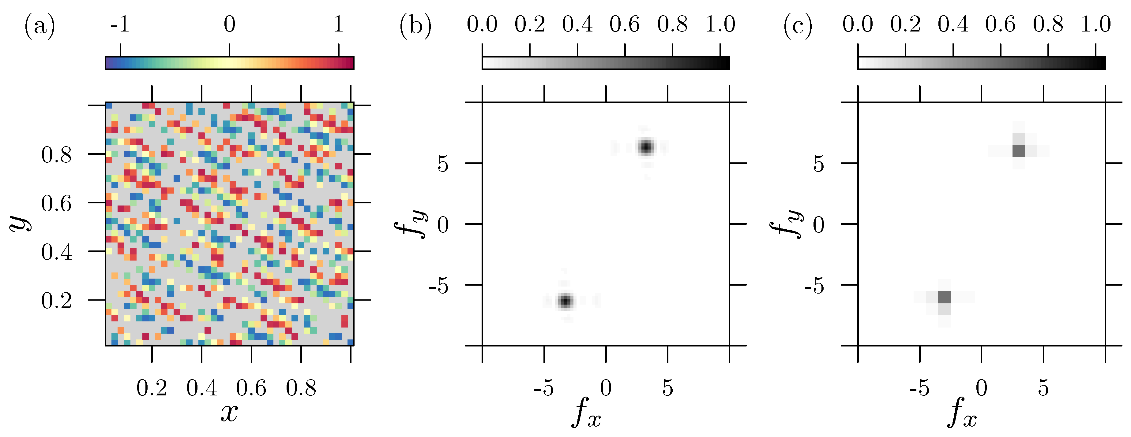
Figure 3.
Sensor data in the co-rotating reference frame. Data is taken as time series from two rotating sensors. The measurement time of the sensor data is folded with its individual phase location, so and describe the two ordinates.
Figure 3.
Sensor data in the co-rotating reference frame. Data is taken as time series from two rotating sensors. The measurement time of the sensor data is folded with its individual phase location, so and describe the two ordinates.
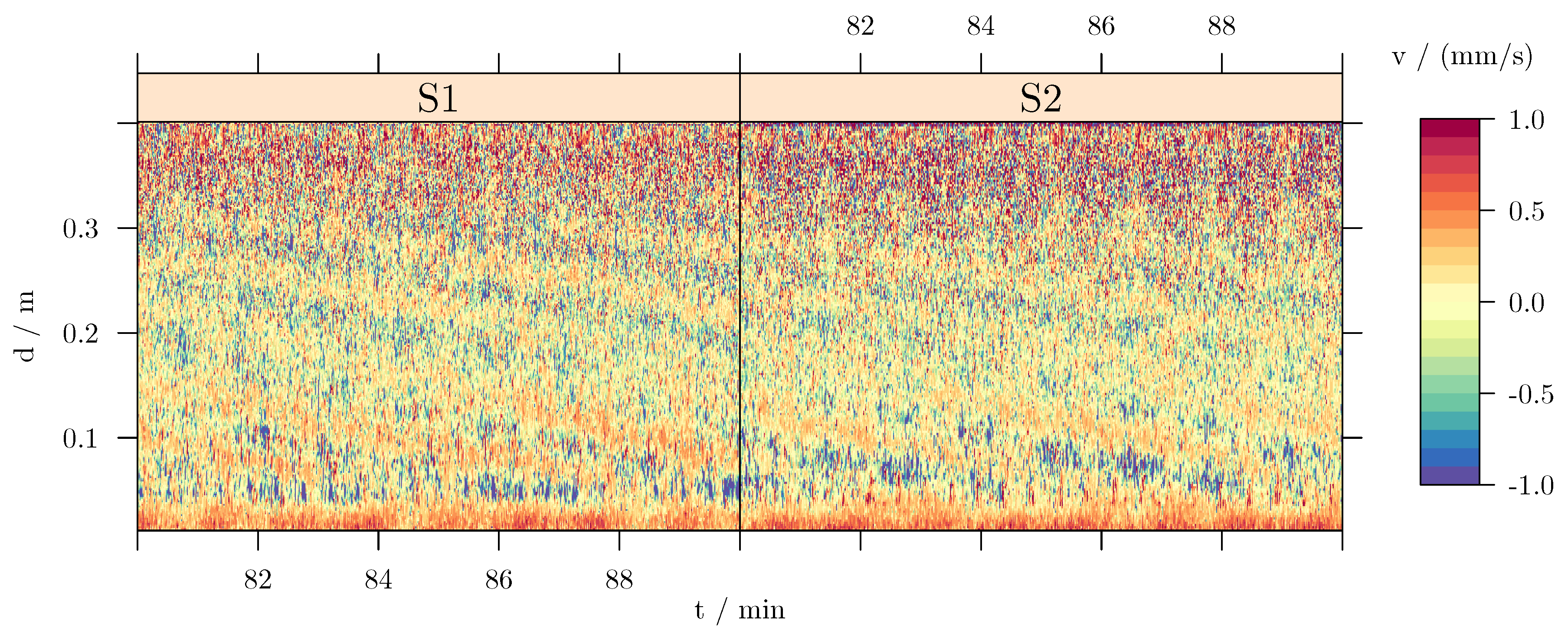
Figure 4.
Spectrum of sensor data. The amplitude spectrum is calculated from the data in Figure 3 with LSM. The weak alias peaks in panel originate from sensor mismatch and aliasing effect due to the outer rotation. The latter acts like a sampling frequency and therefore projects the AMRI wave to .
Figure 4.
Spectrum of sensor data. The amplitude spectrum is calculated from the data in Figure 3 with LSM. The weak alias peaks in panel originate from sensor mismatch and aliasing effect due to the outer rotation. The latter acts like a sampling frequency and therefore projects the AMRI wave to .
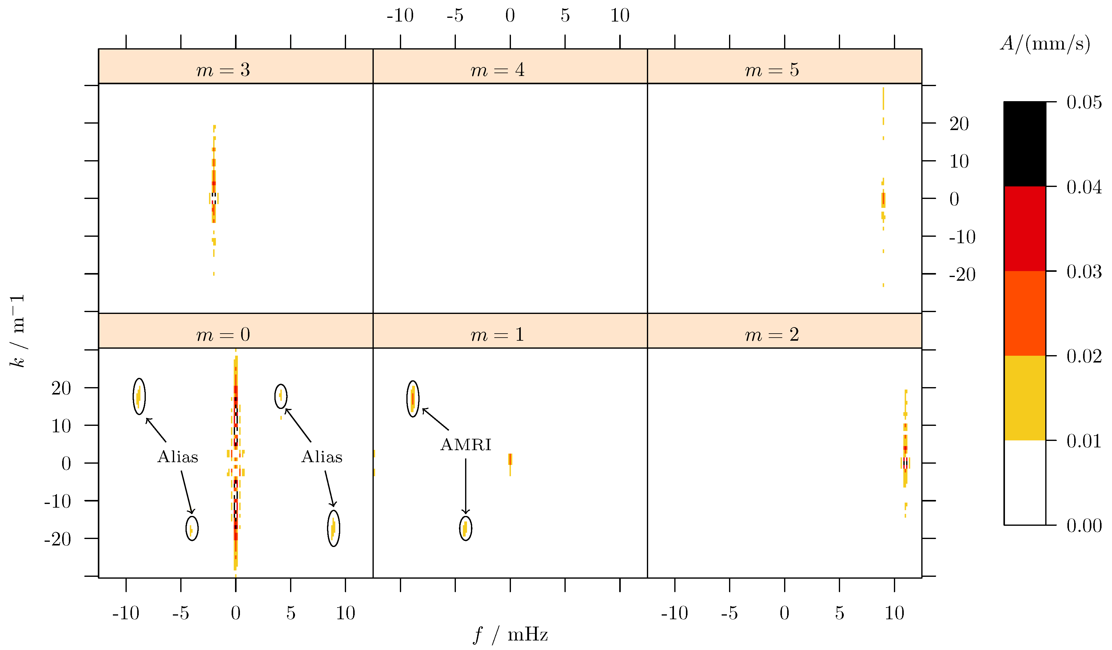
Figure 5.
Butterfly diagram of the Sunspot data. The separation of the individual wings took place according to the proposed procedure presented in Leussu et al. [36]. The colored patches indicate the changing polarity of each cycle. The tilted segmentation lines depict the optimized borders between two cycles.
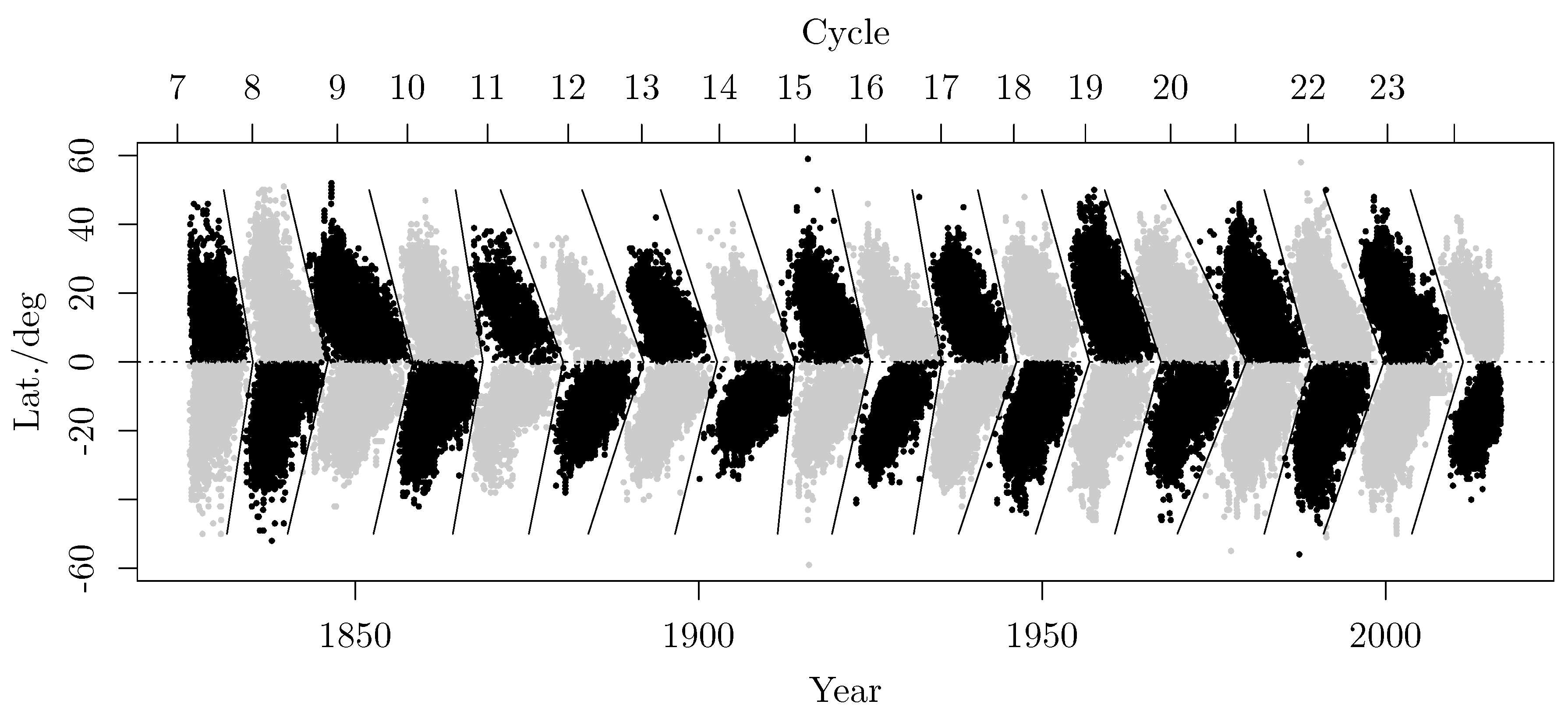
Figure 6.
2D LSM spectrum of the Sunspot data. The curved line follow the path line indicating a wave structure with a certain time dependence. The range of the solar cycle period is given by the vertical dashed gray lines.
Figure 6.
2D LSM spectrum of the Sunspot data. The curved line follow the path line indicating a wave structure with a certain time dependence. The range of the solar cycle period is given by the vertical dashed gray lines.
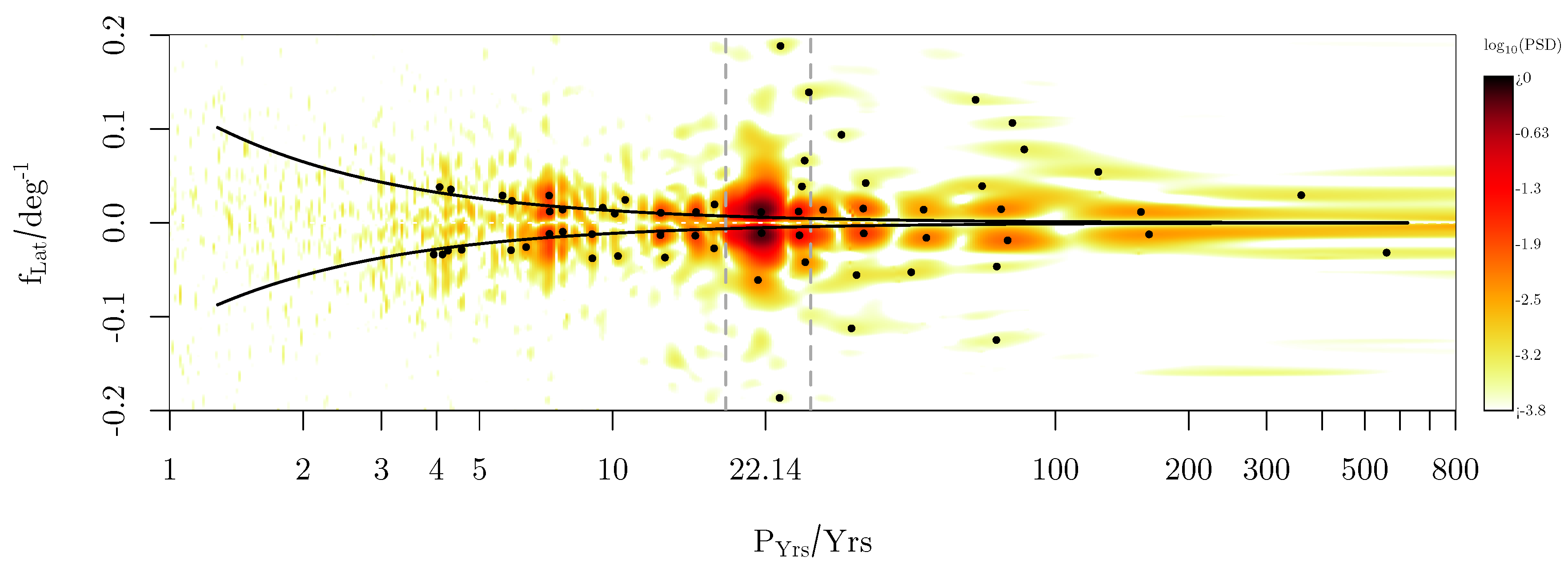

Table 1.
Common Peaks. Period values are given in years. Values above are affected by the low period resolution caused by the limited time span of Sunspot data. The results from Prestes et al. [46] refer to Schwabe cycle and therefore are doubled.
Table 1.
Common Peaks. Period values are given in years. Values above are affected by the low period resolution caused by the limited time span of Sunspot data. The results from Prestes et al. [46] refer to Schwabe cycle and therefore are doubled.
| Process | Common Period | From spectrum | Ref. |
|---|---|---|---|
| Eddy | 515 | 559 | 1 |
| 350 | 359 | 1 | |
| Hale (Schwabe) | 22.14 (11.07) | 21.63 ± 2.5 | 2 |
| 18...28 (2) | |||
| Gleissberg | 88 (80...150) | 78, 85, 125, 156 | 1,2 |
| – | 126 | 125 | 3 |
| – | 2×3.6 | 7.2 | 4 |
| – | 2×3.9 | 7.7 | 4,5 |
Disclaimer/Publisher’s Note: The statements, opinions and data contained in all publications are solely those of the individual author(s) and contributor(s) and not of MDPI and/or the editor(s). MDPI and/or the editor(s) disclaim responsibility for any injury to people or property resulting from any ideas, methods, instructions or products referred to in the content. |
© 2025 by the authors. Licensee MDPI, Basel, Switzerland. This article is an open access article distributed under the terms and conditions of the Creative Commons Attribution (CC BY) license (http://creativecommons.org/licenses/by/4.0/).
Copyright: This open access article is published under a Creative Commons CC BY 4.0 license, which permit the free download, distribution, and reuse, provided that the author and preprint are cited in any reuse.


