
Submitted:
17 September 2025
Posted:
17 September 2025
You are already at the latest version
Abstract
To enhance the position tracking accuracy of heavy-duty asymmetric cylinder electro-hydraulic servo systems subject to unknown matched disturbances, a high-order sliding mode controller with optimal reaching method is proposed, which addresses the robust extension of the classic optimal control problem, which minimizes convergence time under bounded disturbances and system constraints. First, a state-space model of the asymmetric cylinder electro-hydraulic system is established to account for system uncertainties. Second, sliding mode control theory is employed to construct the auxiliary system (i.e., the sliding manifold), and a third-order sliding mode controller with optimal reaching is formulated. Third, Fatou’s Lemma and other theorems are applied to prove that the closed-loop system is globally asymptotically stable under the proposed third-order sliding mode controller with optimal reaching. Finally, a simulation model is built using MATLAB/Simulink. The results demonstrate that, compared with Levant’s third-order sliding mode controller and the quasi-continuous third-order sliding mode controller, the tracking accuracy of the proposed third-order sliding mode controller with optimal reaching is improved by 7 and 8 orders of magnitude, respectively; the convergence time is reduced by factors of 16.6 and 10.2, respectively, and chattering is significantly suppressed.
Keywords:
asymmetric cylinder
; electro-hydraulic system
; high-order sliding mode control
; optimal reaching
1. Introduction
Electro-hydraulic servo systems employ hydraulic fluid as the working medium to facilitate power, motion, and signal transmission through the regulation of pressure energy, flow rate, and flow direction. These systems are characterized by their simpler architecture, compact dimensions, lightweight construction, rapid response, high power density, and ability to enable direct linear motion—attributes that make them indispensable in high-power, high-precision engineering scenarios. Unlike electromechanical systems, their reliance on incompressible hydraulic fluid enables effective force amplification, a critical advantage in applications requiring heavy-load handling. Consequently, they are widely utilized in diverse domains such as robotic arms [1] (for precise end-effector positioning), aircraft simulators [2] (to replicate realistic motion dynamics), vehicle suspensions [3] (for adaptive vibration damping), aerospace engineering [4] (e.g., in flight control actuation), and transportation systems [5] (such as hydraulic braking), thereby demonstrating significant industrial, economic, and scientific research value.
However, electro-hydraulic servo systems are inherently characterized by strong nonlinearity and high-order nonlinear dynamics, stemming from multiple factors: (1) flow-pressure relationships in servo valves, which exhibit nonlinearity due to spool displacement characteristics; (2) fluid compressibility effects, particularly pronounced in long transmission lines, resulting in time-varying bulk modulus; (3) frictional forces (e.g., Coulomb and viscous friction) between the cylinder piston and casing, which induce discontinuous nonlinearities; (4) asymmetric dynamics in single-rod cylinders, where unequal effective areas on either side of the piston result in asymmetric flow gains during extension and retraction. Compounding these complexities, the presence of unknown variable load forces—such as external disturbances in robotic arm operations or varying payloads in vehicle systems—further exacerbates the challenge of achieving precise control.
Over the past few decades, numerous control strategies have been developed to tackle these challenges. Backstepping control [6,7] decomposes complex nonlinear systems into simpler subsystems, enabling stepwise stabilization, but it often imposes computational burdens in high-order systems. Adaptive control [8,9] adapts parameters in real time to mitigate uncertainties but may display slow convergence under rapid load variations. Robust control [10,11] ensures stability under bounded disturbances but typically requires conservative gains, degrading dynamic performance. Hybrid approaches, such as PID-fuzzy [12] or PID-neural network combinations, enhance adaptability but struggle to balance tracking accuracy and robustness in highly nonlinear regimes—particularly in asymmetric cylinder systems, where their fixed parameter-tuning mechanisms cannot accommodate rapid changes in asymmetric flow gains and external disturbances.
Sliding mode control theory (SMC), grounded in modern control principles, offers a compelling alternative by defining a sliding mode switching surface—a hyperplane in the state space—to steer the controlled system toward this surface and maintain motion along it. A key advantage of SMC is its invariance property: once the system enters the sliding mode, its dynamics are determined solely by the design of the switching surface, endowing it with robustness against matched disturbances and parametric uncertainties. However, conventional first-order or second-order SMC has critical limitations: the high-frequency switching inherent to its control signal triggers “chattering” in the system states (i.e., rapid, undesired oscillations around the sliding surface), which accelerates mechanical degradation in hydraulic components (e.g., servo valve spools) and degrades tracking precision [13]. Moreover, the absence of systematic research on optimizing the “reaching phase”—the transition from the system’s initial state to the switching surface—and the subsequent convergence to steady state limits the utilization of SMC’s potential in rapid-response scenarios, where minimization of settling time is paramount.
To address these gaps, this paper presents and assesses a high-order sliding mode controller incorporating an optimal reaching law for asymmetric cylinder electro-hydraulic servo systems. Third-order SMC extends conventional low-order configurations by incorporating higher-order derivatives of the tracking error into the sliding surface, which inherently alleviates chattering by smoothing the control signal (through continuous higher-order switching). This design is particularly well-suited for electro-hydraulic systems, where chattering mitigation is critical to prolonging component lifespan.
Two key challenges associated with this control strategy are addressed:
- Formulating an auxiliary system for the uncertain plant: This system is formulated to encompass the essential dynamics of the asymmetric cylinder, integrating the output variable (e.g., piston displacement) and its first, second, and third time derivatives. By mapping the original system’s nonlinearities and uncertainties into this auxiliary framework, the design of the sliding surface and reaching law is simplified.
- Ensuring optimal performance by solving the “robust Fuller problem”: The Fuller problem, a classic optimal control problem, aims to minimize the time to reach a target state under control constraints. Here, it is extended to a “robust” variant by accounting for the auxiliary system’s constraints and initial conditions [14], thereby ensuring the reaching phase is both rapid and stable despite parametric uncertainties and external disturbances.
The remainder of this paper is structured as follows: Section 2 presents the mathematical model for asymmetric cylinder electro-hydraulic systems, elaborating on the derivation of state-space equations from first principles (including valve dynamics, cylinder flow continuity, and force balance). Section 3 presents the “Robust Fuller Problem” in the context of third-order SMC, presents the solution methodology, and delineates the controller design process with stability guarantees. Section 4 assesses and compares position tracking performance between the proposed controller, Levant’s third-order SMC [29], and quasi-continuous third-order SMC [30] through simulation. Metrics such as root-mean-square (RMS) tracking error, settling time, and chattering amplitude (quantified by control signal variance) are analyzed to validate the superiority of the optimal reaching strategy. Section 5 summarizes the study with a succinct overview of key findings, limitations, and future research directions (e.g., experimental validation on a physical testbed and extension to multi-axis electro-hydraulic systems).
2. Problem Formulation
The schematic of the valve-controlled asymmetric cylinder position servo system is shown in Figure 1. The hydraulic pressure in the rodless chamber, hydraulic pressure in the rod chamber and output displacement y are measured by sensors and fed back to the controller. The controller adjusts the displacement of the servo valve’s main spool to alter the trajectory of the load with mass m, in order to follow the desired trajectory as accurately as possible.
The mechanical equations for the asymmetric cylinder is
where and are the effective areas of the rodless and rodded chambers of the asymmetric cylinder, respectively; is the viscous damping coefficient; is the external loading force; and is the modeling error (including parameters uncertainties, unmodeled friction, among others).
The flow equation of the proportional servo valve is
where and are the flow rates of the rodless and rodded chambers of the asymmetric cylinder, respectively; is the flow gain of the proportional servo valve; is the main spool displacement of the proportional servo valve; and is the system supply pressure. Herein, the signum function can be further expressed as
Since the response frequency of the proportional servo valve is much higher than that of the entire electro-hydraulic servo system, the main spool displacement of the proportional servo valve is approximated as a first-order proportional relationship with the controller’s input voltage, which can be expressed as .where is the displacement-to-voltage gain coefficient of the proportional servo valve’s main spool.
As sealing technology advances, the external leakage coefficient can usually be neglected in the modeling process[15,16,17,18,19,20,21,22,23]; thus, the flow continuity equation for the asymmetric cylinder is
where is the bulk modulus of the hydraulic fluid; and are the initial volumes of the rodless and rodded chambers of the asymmetric cylinder, respectively; is the internal leakage coefficient; and and are the modeling errors of the rodless and rodded chambers of the asymmetric cylinder, respectively (including parameter uncertainties, unmodeled dynamics, among others).
Define the system state variable as
The state-space equation of the asymmetric cylinder system can be expressed as
where
For the valve-controlled asymmetric cylinder electro-hydraulic position servo system addressed in this paper, the following assumptions are made:
1) The desired trajectory is a continuous,bounded and smooth function, and its first-order derivatives, second-order derivatives, and third-order derivatives exist;
2) The hydraulic pressure in the two chambers of the asymmetric cylinder satisfies , where .
3. Controller Design
Figure 2 presents the control structure of the proposed method.
Consider the asymmetric cylinder electro-hydraulic system affine with respect to the control variable
where is a sufficiently smooth objective function. If and are unknown, we refer to (8) is an uncertain system. The order of a sliding mode controller is the minimum order of the time derivatives of the sliding variable in which the control input appears.
where
Let
Then
Assume that and , where , and are positive constants.
The control objective of sliding mode controllers is to reach and maintain the manifold
in finite time. By introducing
where .
Problem 1(Robust Fuller’s Problem) [24]:
The control law for the Robust Fuller’s Problem ensures optimality for the worst-case trajectory under matched bounded perturbations. The worst-case trajectory is such that and .
To solve Robust Fuller’s Problem, we first introduce Fuller’s Problem as follows
Problem 2 (Fuller’s Problem) [24]:
Lemma 1: Assume that . If is an optimal control for Problem 2 with , then an optimal control for problem 1 is given by
Proof of Lemma 1.
Let
We apply the pontryagin’s Maximum Principle [25]. The Hamiltonian function is given
The adjoint system is
Minimization with respect to yields . Thus
Let . Then, (13) reduces to
Since
The optimization can be restricted to . Finally
The solution to Problem 1 has been established in [27]. By using Lemma 1, the solution to the Robust Fuller’s Problem is obtained
where
□
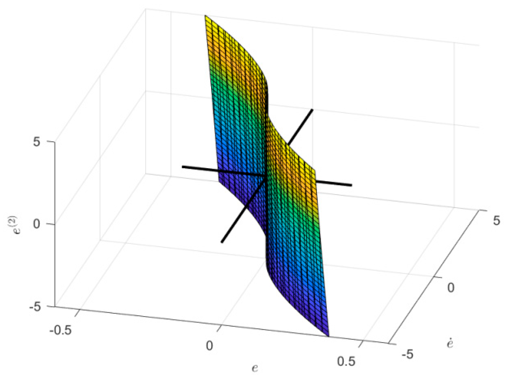
Figure 3.
Switching surface.
Theorem 1. Suppose that . Then, the origin is a uniformly globally finite-time stable equilibrium of system (13) with control law derived from Problem 1.
Proof of Theorem 1.
For any function , denotes a function satisfying
Define a transformation as follows
It is straightforward to verify that
Consider the function
Clearly, we have
These last two properties also imply that is coercive. Given , the system (13) exhibits local finite-time controllability to the origin. Consequently, for any in a neighborhood of the origin, there exists a control function such that the integral on the right-hand side of the definition of can be restricted to a finite interval . Within this interval, remains bounded, ensuring that is bounded in a neighborhood of the origin. Recalling that is homogeneous
Since is bounded in a neighborhood of the origin, the last inequality implies that is bounded on every compact set.
We now demonstrate that is lower semi-continuous. Let denote a sequence of initial conditions converging to and denote a corresponding sequence of optimal solutions. Since is positive and bounded, we can apply the Fatou’s Lemma [28] to obtain
This confirms lower semi-continuity.
Let
is the maximum time required for all the solutions of the differential inclusion (13) reach when starting from any point in .
Define , and observe that
Hence
By the definition of
Now, we have shown makes the origin a globally asymptotically stable equilibrium of system (13).□
4. Simulation Results
In this section, simulations are performed using MATLAB/Simulink to validate the effectiveness of the controller proposed in the previous section. Additionally, the proposed third-order sliding mode controller with optimal reaching (OR) is compared with Levant’s third-order algorithm (L) [29] and quasi-continuous third-order sliding mode algorithm (QC) [30] to verify the superior performance of the proposed method in an asymmetric cylinder electro-hydraulic system.
The system parameters employed in simulations are summarized in Table 1.
The control objective is to regulate the state variable from a specified initial value to track a reference trajectory , subject to matched disturbances . Accordingly, a sliding variable is defined as
Based on the asymmetric cylinder electro-hydraulic system model, the following are derived:
Therefore
such that . To ensure conservatism, are set. Thus, a larger bound is adopted as
To satisfy the conditions of lemma 1, is specified, so that .
Three distinct control laws are denoted as follows:(Levant’s third-order slidingmode controller), (quasi-continuous third-order sliding mode controller) and (third-order sliding mode controller with optimal reaching)
To ensure a fair comparison, is fixed, and and are specified for and . For , only the control amplitude needs to be set.
Simulations are performed over a 0-20s time interval, with results summarized in Figure 4, Figure 5, Figure 6 and Figure 7: red lines correspond to ; purple lines to ; blue lines to . Figure 4 presents the output trajectories of all three controllers alongside the reference trajectory
It is observed from Figure 4 that under , the system output converges to and tracks the desired trajectory after approximately 0.3s with no significant chattering; under , convergence to the target trajectory takes about 0.76s with severe chattering; under , the system remains on the target trajectory from the initial state with no noticeable chattering.
Figure 5, Figure 6 and Figure 7, present the time histories of and for the three controllers, respectively. From these figures, exhibits minimal chattering and the smallest average tracking error compared to and ; the average tracking errors are found to be , respectively. Additionally, in Figure 7, the chattering amplitude of for is larger than that for and , arising from range constraints imposed by nth-order sliding mode control on the nth derivative of the sliding variable (i.e., derivative of the tracking error) [31].
From Figure 4, Figure 5, Figure 6 and Figure 7, exhibits advantages over and in terms of accuracy and convergence time to the reference trajectory. However, the optimal reaching advantage of is not fully apparent when the initial point lies on the desired trajectory. For a more rigorous comparison, with other parameters unchanged, the reference trajectory is reset to and controller activation is delayed by 0.5s.
As shown in Figure 8, takes approximately 1.33s to converge to the reference trajectory from the initial point, takes about 1.01s, and takes only 0.55 seconds. Specifically, converges to the trajectory 0.05 s after activation, which is 16.6 times and 10.2 times faster than and , respectively.
Figure 9, Figure 10 and Figure 11 present the time histories of , and when tracking, respectively. The results are consistent with those for . The average tracking errors of , and after 0.55s are , respectively. From Figure 9, Figure 10 and Figure 11, the significant advantages of in accuracy and optimal reaching are fully verified.
5. Conclusions
1.In this paper, a mathematical model is developed for the asymmetric cylinder electro-hydraulic servo system, and a high-order sliding mode controller is designed for this uncertain system.
2.It is formally proven that the auxiliary system is globally asymptotically stable under the proposed third-order sliding mode controller.
3. A simulation model based on MATLAB/Simulink is constructed, and simulations confirmed that the third-order sliding mode controller exhibited a smaller absolute average tracking error (m). Compared with Levant’s third-order sliding mode controller and the quasi-continuous third-order sliding mode controller, the tracking accuracy of the proposed third-order sliding mode controller is improved by 7 and 8 orders of magnitude, respectively; the convergence time is reduced by factors of 16.6 and 10.2, respectively; and it demonstrates superior chattering suppression capability.
Author Contributions
Theoretical analysis: P.W. and Y.W.; designing experiments and analyzing data: P.W and J.Y.; conducting simulations: P.W. and Y.W.; writing the paper: P.W.; revising the paper: P.W and J.Y. All authors have read and agreed to the published version of the manuscript.
Funding
This work is supported by the Natural Science Foundation of Jiangsu Province (Grant No. BK20241640) and Scientific Research Project of Anhui Higher Education Institutions (Grant No. 2023AH053087).
Data Availability Statement
The datasets generated during and/or analysed during the current study are available from the corresponding author on reasonable request.
Acknowledgments
During the preparation of this manuscript, the authors used MATLAB for the purposes of simulation. The authors have reviewed and edited the output and take full responsibility for the content of this publication.
Conflicts of Interest
The authors declare no conflicts of interest.
Abbreviations
The following abbreviations are used in this manuscript:
| OR | Third-order sliding mode controller with optimal reaching |
| L | Levant’s third-order algorithm |
| QC | Quasi-continuous third-order sliding mode algorithm |
References
- Jing, Baorui. Unknown System Dynamics Estimator for Motion Control of Nonlinear Robotic Systems. IEEE Transactions on Industrial Electronics 2020; 67: 3850-3859. [CrossRef]
- Han JS. Friction compensation for low velocity control of hydraulic flight motion simulator: a simple adaptive robust approach. Chinese Journal of Aeronautics 2013; 26: 814-822.
- Huang Y, Na J, Wu X, et al. Approximation-Free Control for Vehicle Active Suspensions With Hydraulic Actuator. IEEE Transactions on Industrial Electronics 2018; 65: 7258-7267. [CrossRef]
- Tu JY, Lin PY, Stoten DP, et al. Testing of dynamically substructured, base-isolated system using adaptive control techniques. Earthquake Engineering & Structural Dynamics 2009; 39: 661-681. [CrossRef]
- Donner R. Emergence of Synchronization in Transportation Networks with Biologically Inspired Decentralized Control. Springer Berlin Heidelberg 2009; pp.237-275.
- Won D, Kim W, Shin D, et al. High-Gain Disturbance Observer-Based Backstepping Control With Output Tracking Error Constraint for Electro-Hydraulic Systems. IEEE Transactions on Control Systems Technology 2015; 23: 787-795. [CrossRef]
- Guo Q, Zhang Y, Branko G. Celler, et al. Backstepping Control of Electro-Hydraulic System Based on Extended State Observer With Plant Dynamics Largely Unknown. IEEE Transactions on Industrial Electronics 2016; 63: 6909-6920. [CrossRef]
- Wang C, Quan L, Jiao Z, et al. Nonlinear adaptive control of hydraulic system with observing and compensating mismatching uncertainties. IEEE Trans. Control Syst. Technol 2018; 26: 927–938. [CrossRef]
- Li X, Yao J, Zhou C. Adaptive robust output-feedback motion control of hydraulic actuators. Int. J. Adapt. Control Signal Process 2017; 31: 1544–1566. [CrossRef]
- Bakhshande F, Bach R, Sffker D. Robust control of a hydraulic cylinder using an observer-based sliding mode control: Theoretical development and experimental validation-ScienceDirect. Control Engineering Practice 2020; 95:104272. [CrossRef]
- Shen W, Jiang J, Karimi H R, et al. Observer-Based Robust Control for Hydraulic Velocity Control System. Mathematical Problems in Engineering 2013; 689132. [CrossRef]
- Wang YF, Ding H, Zhao J, et al. Neural network-based output synchronization control for multi-actuator system. International journal of adaptive control and signal processing 2022; 36: 1155-1171. [CrossRef]
- Utkin V ,Guldner, Jürgen, et al. Sliding Mode Control in Electro-Mechanical Systems, Second Edition. Crc Press 2009; 619:455-475. [CrossRef]
- G. Bartolini, A. Ferrara, A. Levant, et al. On second order sliding mode controllers. Variable Structure Systems, Sliding Mode and Nonlinear Control, ser. Lecture Notes in Control and Information Series, K. D. Young and U. Ozguner, Eds. London, U.K.: Springer Verlag 1999; pp.329–350.
- Yao B, Al-Majed M. High-performance robust motion control of machine tools: an adaptive robust control approach and comparative experiments. IEEE/ASME Transactions on Mechatronics 1997; 2: 63-76. [CrossRef]
- Guo K, Wei J, Fang J, et al. Position tracking control of electro-hydraulic single-rod actuator based on an extended disturbance observer. Mechatronics 2015; 27:47-56. [CrossRef]
- Won D, Kim W, Shin D, et al. High-Gain Disturbance Observer-Based Backstepping Control With Output Tracking Error Constraint for Electro-Hydraulic Systems. IEEE Transactions on Control Systems Technology 2015, 23: 787-795. [CrossRef]
- Guo Q, Yin JM, Yu T, et al. Coupled-disturbance-observer-based position tracking control for a cascade electro-hydraulic system. Isa Trans 2017; 68: 367-380. [CrossRef]
- Wang B, Zhang N, Ji H. Study on Precise Displacement Control of a Miniature Hydraulic System via RBF-DOB. IEEE Access 2018, 6: 69162-69171. [CrossRef]
- Xu ZB, Ma DW, Yao JY. Uniform robust exact differentiator based adaptive robust control for a class of nonlinear systems. Transactions of the Institute of Measurement and Control 2018, 40: 2901-2911. [CrossRef]
- Guo Q, Li X, Jiang D. Full-state Error Constraints Based Dynamic Surface Control of Electro-hydraulic System. IEEE Access 2018, PP. 1-1. [CrossRef]
- JI X hao, WANG Cheng wen, CHEN Shuai, et al. Sliding mode back-stepping control method for valve-controlled electro-hydraulic position servo system[J]. Journal of Central South University 2020, 51: 1518−1525.
- Xiong Y, Wei J, Feng R, et al. Disturbance observer based pressure control for electrohydraulic system. Journal of Central South University 2017, 48: 1182-1189.
- A.T. Fuller. Relay control systems optimized for various performance criteria. IFAC Proceedings Volumes 1961,1: 520-529. [CrossRef]
- Pontrjagin L S. The Mathematical Theory of Optimal Processes. Interscience 1962, 16: 493-494.
- G. Bartolini, A. Ferrara, E. Usai and V. I. Utkin. On multi-input chattering-free second-order sliding mode control. IEEE Transactions on Automatic Control 2000, 45: 1711-1717. [CrossRef]
- A. A. Feldbaum. On synthesis of optimal systems with the help of phase space. Avtomatika i telemehanika 1955, 16: 129–149.
- Apelian C, Surace S, Mathew A. Real and Complex Analysis. McGraw-Hill 2009.
- Levant A. Universal single-input-single-output (SISO) sliding-mode controllers with finite-time convergence. IEEE Transactions on Automatic Control 2001, 46: 1447-1451. [CrossRef]
- Levant A. Quasi-Continuous High-Order Sliding-Mode Controllers. IEEE Transactions on Automatic Control 2005, 50: 1812-1816. [CrossRef]
- F. Dinuzzo, A. Ferrara. Higher Order Sliding Mode Controllers With Optimal Reaching. IEEE Transactions on Automatic Control 2009, 54: 2126-2136. [CrossRef]
Figure 1.
Schematic of the asymmetric cylinder system.
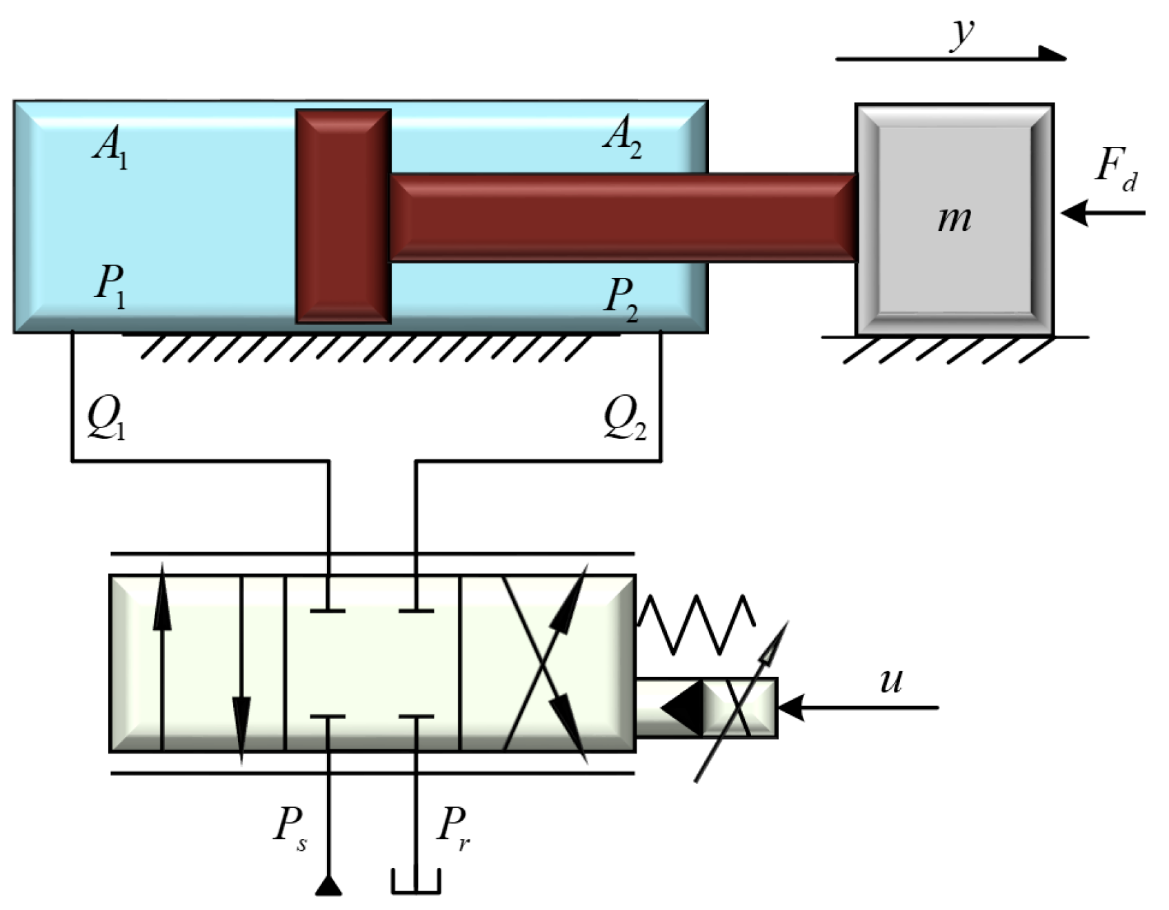
Figure 2.
Block diagram of the proposed controller.
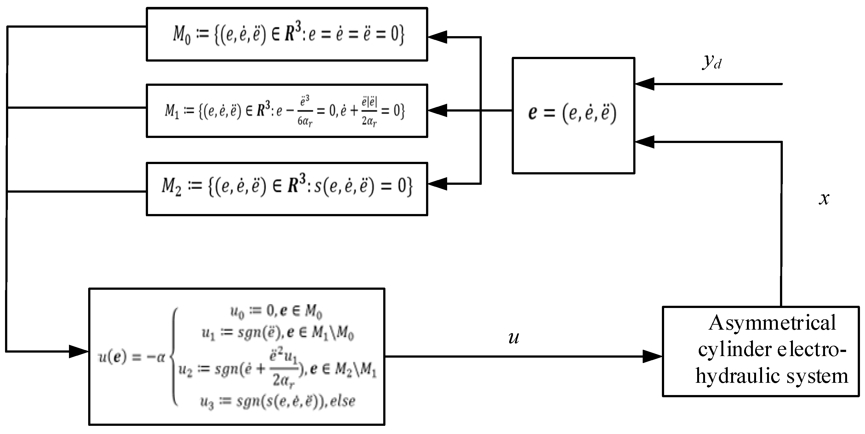
Figure 4.
Output Trajectory of different methods.
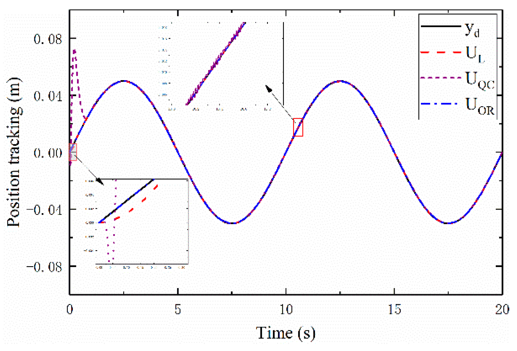
Figure 5.
Sliding variable versus time.
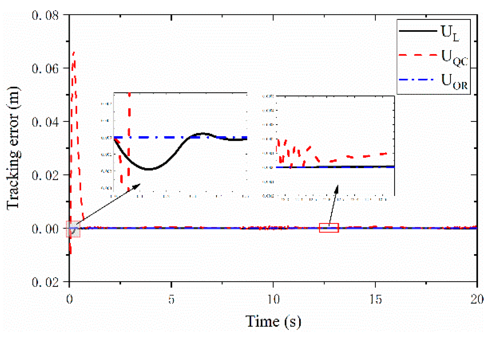
Figure 6.
The first order derivative of a sliding variable versus time.
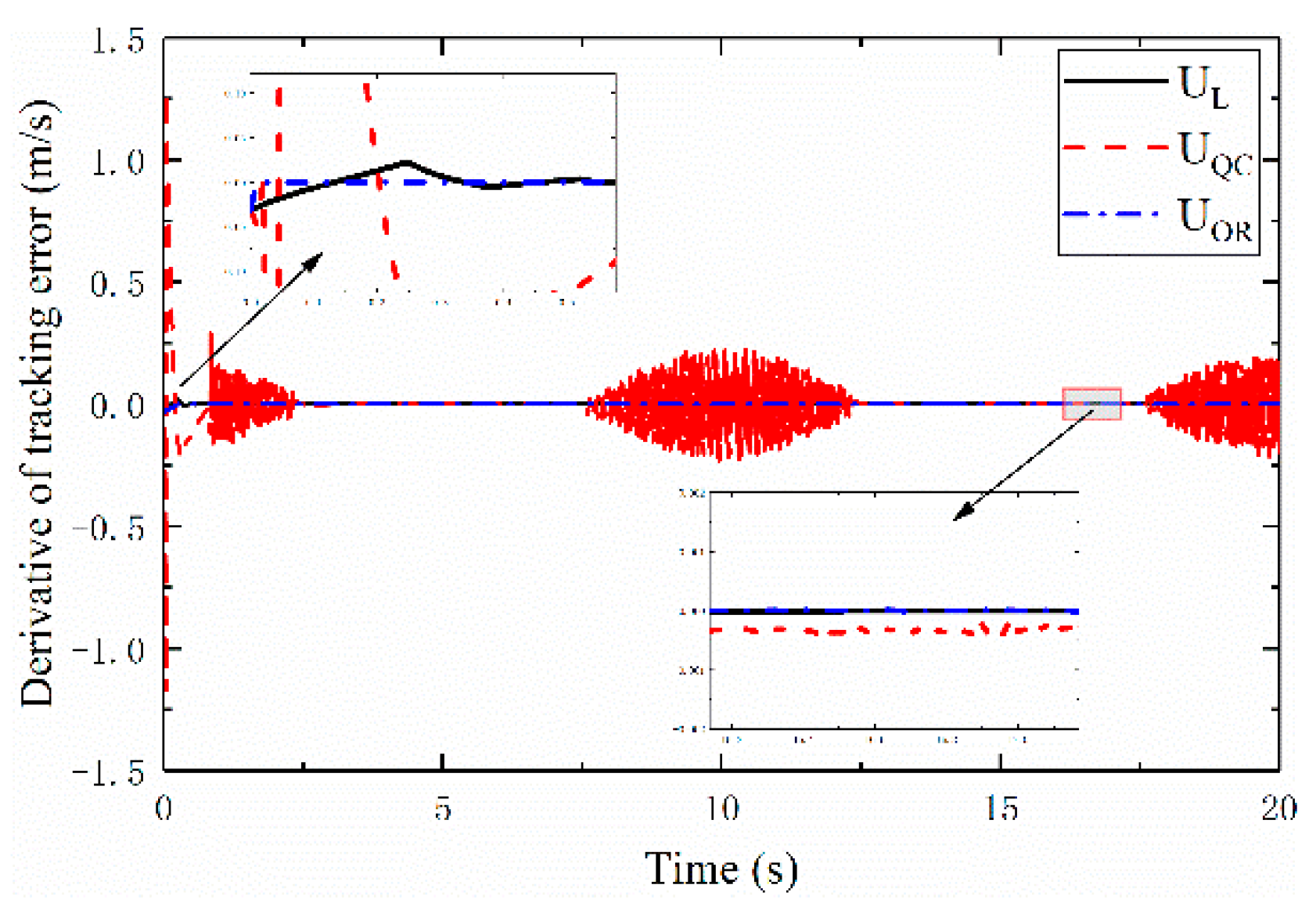
Figure 7.
The second order derivative of a sliding variable versus time.
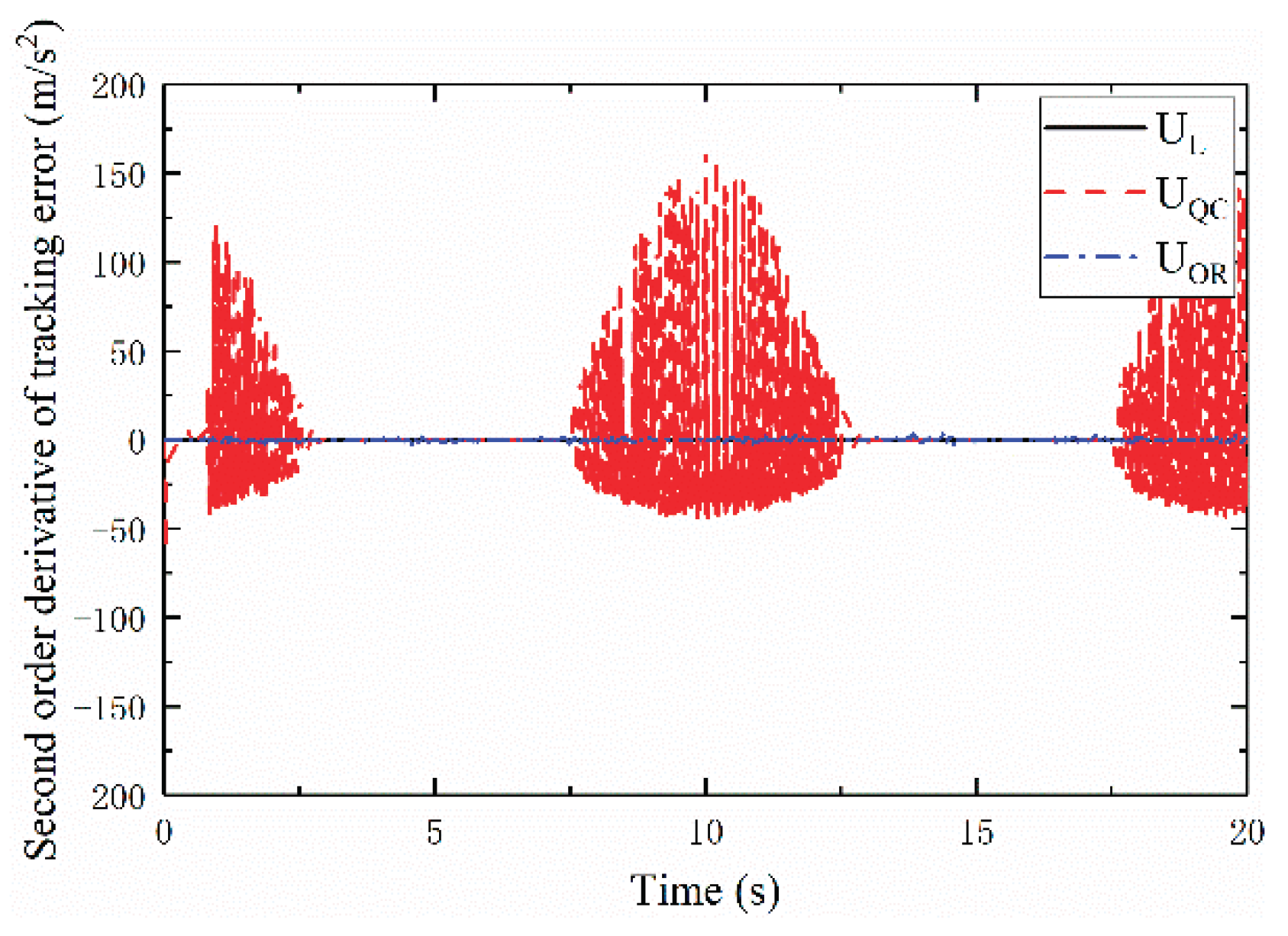
Figure 8.
Output Trajectory of different methods.
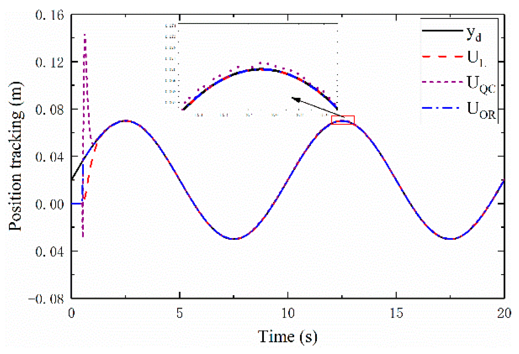
Figure 9.
Sliding variable versus time.
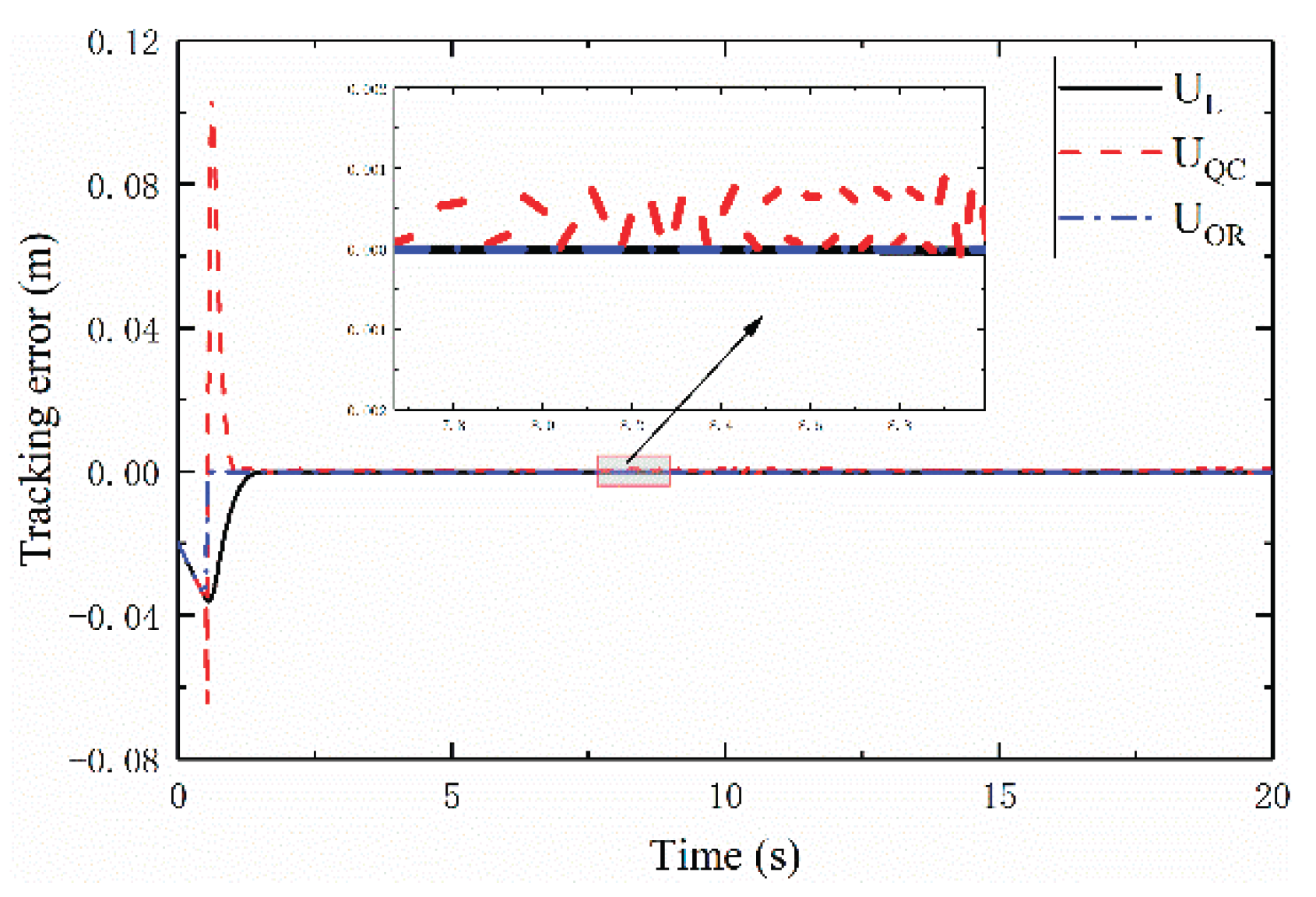
Figure 10.
The first order derivative of a sliding variable versus time.
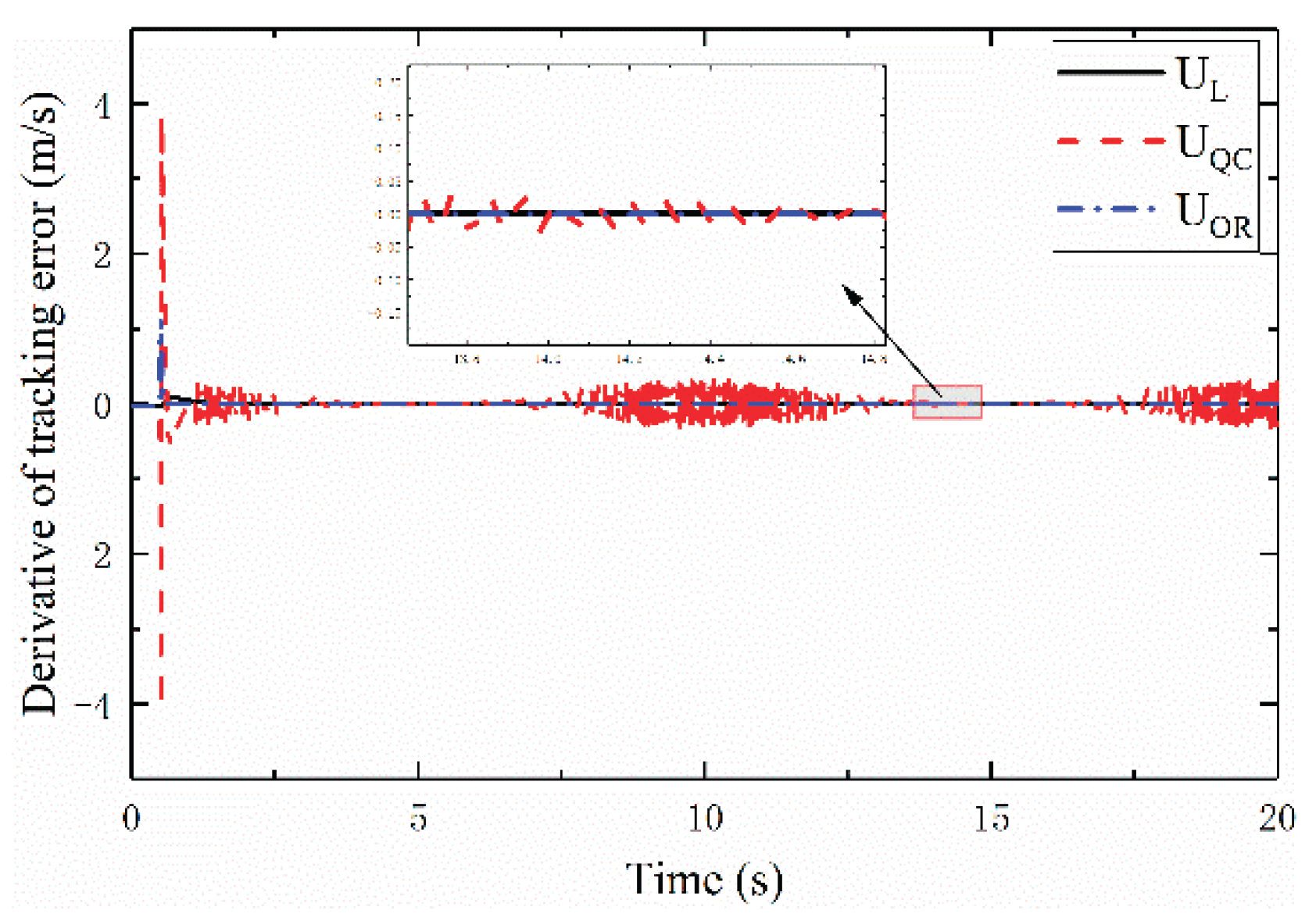
Figure 11.
The second order derivative of a sliding variable versus time.
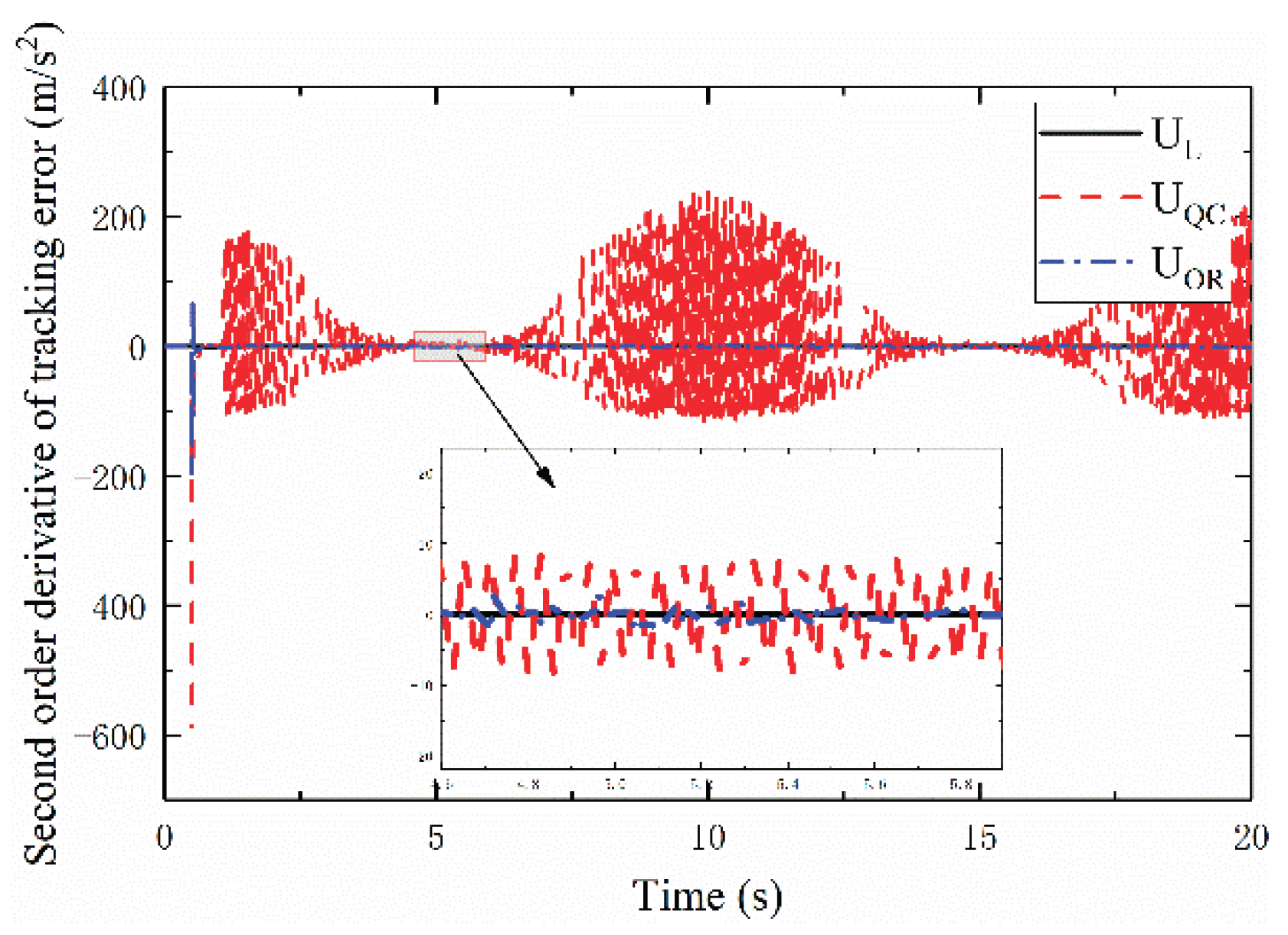

Table 1.
Parameters of asymmetric cylinder system.
| parameters | value |
|---|---|
| m/kg | 320 |
| Ps/Pa | 14*106 |
| Pr/Pa | 0 |
| b/(NM) | 2000 |
| A1/m2 | 0.0314 |
| A2/m2 | 0.016014 |
| V01/m3 | 0.015 |
| V02/m3 | 0.008 |
| /Pa | 7*108 |
| Ct/(m3sPa) | 4*10-13 |
| k1/(m3sVPa1/2) | 8.91*10-8 |
Disclaimer/Publisher’s Note: The statements, opinions and data contained in all publications are solely those of the individual author(s) and contributor(s) and not of MDPI and/or the editor(s). MDPI and/or the editor(s) disclaim responsibility for any injury to people or property resulting from any ideas, methods, instructions or products referred to in the content. |
© 2025 by the authors. Licensee MDPI, Basel, Switzerland. This article is an open access article distributed under the terms and conditions of the Creative Commons Attribution (CC BY) license (http://creativecommons.org/licenses/by/4.0/).
Copyright: This open access article is published under a Creative Commons CC BY 4.0 license, which permit the free download, distribution, and reuse, provided that the author and preprint are cited in any reuse.


