On Scientific Discovery–A Decision-Machine Approach

Lizhi Xin; Kevin Xin

doi:10.20944/preprints202509.1400.v1

Submitted:

16 September 2025

Posted:

16 September 2025

Read the latest preprint version here

Abstract

The traditional approach to scientific discovery has strictly followed an entity – property – structure –> function –> numerical value one, an approach that has sought to seek out the "terminal" structure of nature; we've developed a decision-machine that sets out conducting scientific discovery "following" an event – information – operation –> matrix –> vector approach with an emphasis on simulating nature's behavior. By defining three induction rules for the decision-machine to obey: 1) similarity degree, 2) effective operational level, and 3) consistency, the decision-machine is able to ensure the effectiveness of inductive reasoning. This way, the decision-machine has a slight advantage over human scientists in three areas: being able to keep a "cool head" and not be influenced by emotions (objectivity), not being dragged into endless debate of whether potential hypothesizes are viable (effectiveness), and being able to work around the clock nonstop continually self-learning and self-adapting (automation). The decision-machine is constructed by drawing upon the concept of quantum superposition and Darwinian natural selection; superposition is used to generate all the possibilities of the real world (mother nature's choices), then natural selection is utilized to evolve the "fittest" hypothesis that most approximately conforms to the real world, and lastly through means of recursive learning, the decision-machine is able to dynamically “deal with” the unknown of the future.

Keywords:

scientific discovery

;

decision-machine

;

quantum superposition

;

natural selection

;

quantum-like evolutionary algorithm

;

genetic programming

;

inductive rules

Subject:

Physical Sciences - Other

I. INTRODUCTION

In simplest terms the essence of scientific discovery is to seek out the laws of nature [1,2,3].

The four key elements of scientific discovery are:

1): Nature – The object of scientific discovery; the universe composed of infinitely many potential possible worlds.
2): Observer – The subject of scientific discovery; to design the apparatus, conduct measurements, record the results, and to propose potential hypothesis that interprets what is being observed.
3): Measuring instrument – The tools of scientific discovery; to interact with nature and to project the infinitely many potential possible worlds into the real world, i.e. a set of observational data.
4): Observed data – The target of scientific discovery (real world); the data projected by the apparatus.

Scientific discovery from the observer’s perspective is to find the regularities from the observed data recorded by the measuring apparatus. In other words, the observer postulates multiple hypotheses based on observation data to understand and explain natural phenomena. The scientific hypotheses proposed are the observer’s attempts to discover repeating patterns from observed data, and these patterns conform to the consistent rules applied by the observer to reconstruct the past and predict the future of nature.

The modern-day scientific discovery is of a reductionist process, i.e. an entity – properties – structure approach is used to describe the essence of nature; the reductionist process is based off a conceptual framework which establishes a symbolic formal system (mathematical language) to describe rules that represent the laws of nature.

The typical example of scientific discovery is the question of how does the temporal evolution of an entity takes place? In other words: how does the entity go from one point to another? For an entity at a certain time

t_{i}

, it is observed at point A, position is

x_{i}

; then at time

t_{j}

, it is observed at point B, where its position is at

x_{j}

.

Thus, how do we describe the kinetic laws of an entity's movement from point A to point B?

How an entity goes from A to B is essentially a “problem” of choosing which path (real world) to take from the infinite possible ones (potential worlds). The real world as observed by the observer is the path the entity chose, i.e. the time series of the entity's position that the apparatus records. The mission of the observer in scientific discovery is to find the regularities from observed time series data.

Modern-day physical science mainly describes how the entity chooses which path to take based on two conceptual frameworks [4,5,6]:

1): Force – differential equations: the observer first finds a differential equation to describe the entity's movement; then under the constraints of the initial and boundary conditions, the integral obtains a function to describe the trajectory of the entity's movement.
2): Energy – principle of least action: given all the potential paths that the entity can take, the observer calculates the Lagrangian (kinetic energy - potential energy) of each path and the one with the smallest Lagrangian is the one that the entity chooses.

When mother nature can be fully described in terms of the conceptual framework of force or energy with causality, we can completely determine the current, past, and future trajectory of an entity by using Newtonian mechanics or Lagrangian least action. However, the real world is complex and most times is non-linear, mother nature acts as she wishes, we don’t have the ability to “command” mother nature to act like the mechanical movement tick ticking of a clock.

When the entity is under ideal conditions without external “disturbance”, Newtonian mechanics and principle of least action can formulate a function to completely determine the trajectory of the entity. But we know that in the real world, the entity is always interacting with other entities; the pollen floating in water “swims” around randomly due to colliding with molecules; because the electrons are “disturbed” by the measuring apparatus, according to quantum mechanics electrons cease to have a trajectory; in summary, both the trajectory of pollen in Brownian motion and the electron cannot be described by a function with complete certainty, thus, we can say that we don’t know which path the pollen or electrons will “chose”. By using the Boltzmann distribution and diffusion equation, Einstein described the random drifting of the pollen, and he calculated the probability of where the pollen will be at a given time [7]; by “imagining” an electron simultaneously “walking” on every possible path, Feynmann proposed path integral to calculate the probability of an electron being in what position at a given time by weighted sum of all possible paths for the electron [8,9]. Of course, an electron cannot be on every single possible path at once, or pass through both slits simultaneously of the double slit experiment, and Schrodinger’s poor cat won’t be dead and alive at the same time [10]; naturally that begs the question: where is the precise boundary between the macroscopic and microscopic “worlds”? Under the current conceptual framework this question is unanswerable, it’s been 100 years and this question is still open.

An entity’s motion at the classical, molecular, and atomic level can be summarized as follows:

1): Freefalling apple: The entity’s position is completely certain that’s described by a function (Newton Mechanics or Principle of Least Action).
2): Pollen: Due to the uncertain initial conditions of all the molecules, the position of the pollen can only be predicted probabilistically (Boltzmann distribution and diffusion equation).
3): Electron: Because the process of the interactions between the electrons and the measuring apparatus is unknown, the position of the electron can only be predicted probabilistically (Path-integral, Schrodinger equation, Heisenberg matrix mechanics).

Under the current known conceptual framework, the entity – property – structure approach can’t answer the question of where the macro-micro boundary is, and it also can’t answer the question of path-selection.

For scientific discovery, what will happen if a transformation from an entity – property – structure approach to an event – information – operation approach takes place?

Under the event – information – operation approach [11,12,13], the trajectory of the entity is not determined by a “mysterious” function, but is regarded as a series of events “performed” by nature: a certain point at a given time, the entity “performs” an operation along the motion curve (a) upward or downward movement (b) move a certain distance. We don’t consider the entity’s movement as a simple state (position) numerical value change, but to consider it as a process of a set of events that occur following a certain rule. The entity is undergoing a movement of creative evolution, which now the entity’s movement is a dynamic view of infinite possibilities, not a static mechanical one.

Therefore, we can unifying describe the movement of a freefalling apple, pollen, and the electron all together under an event – information – operation approach:

1): Freefalling apple (classical-level): Mother nature provides complete information; the trajectory is completely certain.
2): Pollen (molecule-level): The observer does not have complete information regarding the movement of all the molecules; the trajectory is uncertain (Human ignorance).
3): Electron (atomic-level): Mother nature provides incomplete information regarding the electron; the trajectory is uncertain (Mother nature’s “ignorance”).

How do we predict the possible future events of the entity from its already-happened past event series'?

Scientific discovery then becomes a process of reconstructing the past series of events and to attempt to reasonably predict possible future events, one that becomes an induction of known to unknown, past to future.

Scientific discovery based on the event – information – operation approach has three main elements:

1): Nature: the natural phenomena that repeatedly occurs can be "seen" as some "operation" that nature "performs", and these "operations" are what causes a series of events to be triggered; one event after another event in which these repeatedly happening events may have a certain regularity.
2): Observer: the observer learns from the recurring events, trying to find patterns, and from what they learned to predict future possible events.
3): Information: nature continuously presents these recurring events as “hints” to its patterns, while the observer continuously attempts to find effective information from these “hints” presented by nature.

Based on the event – information – operation approach, the fundamentals of scientific discovery for the observer are the projection of the observer’s beliefs that one event will happen after another. Naturally the question that’s asked is how effective are the projections of the observer's beliefs? Thus, we find ourselves faced with Hume’s Problem of Induction [14,15], in which the main problem: is the observer’s inductive reasoning effective enough?

Hume correctly pointed out, when predicting future events that have not been observed yet, future events cannot be logically deduced from past events that have already happened, because past events don’t have a logical cause and effect on future events, we can only “guess” what may happen. In regards to why one is chosen from the possibilities and not the others, Hume said it’s just a matter of “habit” in the minds of observers based on recurring events. Even though the Problem of Induction indicates that is impossible to predict the future with 100% accuracy, but Hume elucidated the mechanism of how observers' make predictions, i.e. formulating inductive rules about what might happen based on past events, then the observer makes predictions following the rules of induction formulated in their beliefs.

Thus, how do we validate the effectiveness of the inductive rules?

To answer this, it is crucial for the observer to be able to consistently make reasonable predictions. What's important is the effectiveness of induction, which doesn't necessarily mean that predictions will be 100% accurate, since no one can make accurate predictions of future in the first place; the observer’s beliefs will be solidified if the prediction is correct (the result matches with what was being predicted), and will be hampered if they are wrong, in which the observer will readjust their beliefs, all the while learning from those mistakes to improve the accuracy of future predictions.

If the real world that is observed by us is considered the "chosen one" of nature (the one that is "selected" from all the possible worlds), then the scientific discovery process of nature's "chosen one" calls for the observer to be provided with a set of inductive rules to make corresponding choices. The remaining task is to validate the effectiveness of induction in order to assure that the observer can conduct scientific discovery consistently and reasonably. Specifically, the inductive rules can be quantified by a group of clearly defined numerical values', in which the observer can then apply these inductive rules to consistently reconstruct the past as well as reasonably predict the future. Here we define two numerical values of “similarity degree” and “effective operational level” to quantify the effectiveness of inductive rules:

1): Similarity degree: The similarity of the reconstructed world and the real world.
2): Effective operational level: How confident the observer is when making predictions and how accurate the observer’s predictions are.

In this paper, we construct a decision-machine that can conduct operations on observed data based on a clearly defined set of inductive rules, and by obeying said rules the decision-machine is able to approximately accurately reconstruct nature's “chosen one” (real world), and to reasonably predict what will happen in the future. The decision-machine will obey the inductive rules of 1) similarity degree, 2) effective operational level, to conduct inductive reasoning consistently.

The specific steps of the decision-machine to conduct scientific discovery are:

1): Randomly generate many possible “worlds”.
2): Calculate the similarity of each generated possible “world”.
3): Apply the effective operation (the one with the greatest similarity degree) to consistently predict the future.

The possibility of the decision-machine being able to reconstruct mother nature's "chosen one" (real world) from the randomly generated possible "worlds" is quite low, if not impossible. In order to improve the "similarity degree" of the decision-machine's generated possible “worlds” in comparison to nature's "chosen" real world, Darwinian principle of natural selection is applied to do so. Through means of crossover, selection, and mutation, the decision-machine utilizes the evolutionary algorithm to optimize the “similarity degree” of the generated possible “worlds” with the real world; after generations of evolution, the evolutionary algorithm will gradually improve the “similarity degree” between the generated possible “worlds” with the real world, and lastly the one possible "world" with the highest "similarity degree" produced by the decision-machine's operation is the said operation that's utilized as the most effective one to reasonably predict the future.

We firmly believe that for scientific discovery it's crucial to find the most valuable information from observed data. The current way of scientific discovery overly emphasizes the computation of numerical value of the entity’s properties and neglects the actual change of the entity’s movement; or in other words there is an emphasis more on nature’s structure (described by mathematical equations) rather than nature’s “behavior” (described by event rules); because most of the time nature will not manifest all of its valuable information in entirety, it's difficult if not impossible for us to discover a clearly defined structure of nature. So, we’ve constructed a decision-machine to “compete” with mother nature to find a set of rules that govern “her” behaviors: if nature provides us complete information, then the decision-machine will find a pure strategy to completely simulate nature’s behavior; if nature "flips" a coin, then the decision-machine will counter by using a mixed strategy to "flip a coin back" which should simulate nature's behavior in the most approximate way possible [16].

If mother nature has a simple structure hidden somewhere, then we just need to patiently wait for the next “Einstein” to surprise us by finding it; but if nature is constantly creatively evolving, then we are faced with the ignorance of nature (the unknown of the unknown), then the decision-machine can "game" with nature, in which by constantly self-evolving as well as self-adaptively learning effectively aids us in the scientific discovery process of simulating mother nature's "behaviors".

II. METHODS

The decision-machine approach for scientific discovery consists of three parts:

1): $X : \{x_{1}, x_{2}, \dots, x_{n}\} :$ Observed data, the target of scientific discovery by decision-machine
2): $H : \{h_{1}, h_{2}, \dots, h_{n}\} :$ Scientific hypothesis, the decision-machine puts forth different hypothesis based on the observed data $X$ .
3): $V : \{v_{1}, v_{2}, \dots, v_{n}\} :$ Evaluation criteria, the performance of each proposed hypothesis $H$ by the decision-machine is evaluated based on the observed data $X$ .

Based on the current circumstances of the historical data, scientific discovery is then essentially finding the most “satisfactory” hypothesis

h \in H

to reconstruct observed data X and predict the future. Mainstream scientific discovery based on the entity – property – structure approach is to find the kinetic laws of the entity from observed data as described in (1), i.e. to use a function to determine the entity’s motion trajectory of the past, present, and future.

x (t + 1) = f (x (t), B (t))

(1)

where

x (t)

is the position of the entity and

B (t)

is the properties of the entity. Unless under ideal circumstances where the trajectory of a classical object can be completely mapped like a freefalling apple, the same cannot be said for an entity of a complex non-linear system, the trajectory under these circumstances can't be completely obtained due to uncertainty, like in the case of the pollen and electron.

It can be said that the main problem for scientific discovery as a whole arises from incomplete information; therefore, from an information perspective, the decision-machine will conduct scientific discovery with the event – information – operation approach. What an event presents to the decision-machine is information not property. Unlike mainstream methodologies that attempt to discover the laws of nature with some corresponding structure through the entities' properties, the decision-machine considers observed data (

X : \{x_{n}\}

: motion curve) as a series of events "executed" by mother nature performing some "action"; mother nature's "action" consists of two parts: a) the entity either "crawls" upwards or downwards along the curve of the graph; b) the entity moves a said distance between two observation points.

The decision-machine can now start to simulate nature's "behavior". At any given point, the decision-machine performs an operation to simulate nature's behavior by: a) decide if the entity will "crawl" upwards or downwards; b) calculate the absolute value of the distance between two observed points. After doing the above, a simulated trajectory of the entity (possible worlds) is now generated by the decision-machine. The "action" that the decision-machine "decides to take" is based on the information it obtains from learning the observed data

X : \{x_{n}\}

, thus the decision-machine will generate different simulated trajectories (possible worlds) from the different information it obtains, therefore, the decision-machine discovers the kinetic laws of the entity as (2).

x^{'} (t + 1) = \{\begin{matrix} x^{'} (t) + Δ x_{t, t + 1}^{'}, d = 0 \\ x^{'} (t) - Δ x_{t, t + 1}^{'}, d = 1 \end{matrix}

(2)

where d=0 represents that the decision-machine predicts that the entity will “crawl” upwards on the curve of the graph; d=1 represents that the decision-machine predicts that the entity will “crawl” downwards on the curve of the graph;

Δ x_{t, t + 1}^{'} = |x^{'} (t + 1) - x^{'} (t)|

is the distance between two observation points as calculated by the decision-machine.

The scientific discovery of the decision-machine can be described by the (Q event, A operation, R expected return) framework as (3).

{D M}_{V : \{v_{n}\}} \overset{H : \{h_{n}\}}{\to} [Q, A, R]

(3)

where DM is the decision-machine;

H : \{h_{n}\}

are the decision-machine's proposed hypothesizes;

V : \{v_{n}\}

is the criteria used to evaluate the performance of each proposed hypothesis; event (Q), operation (A), and expected return (R) are utilized by the decision-machine to conduct scientific discovery, which are defined as:

1): Q: $\{(q_{1} | q_{2}, Δ x_{k - 1, k}), k = 1, \dots, N\}$ ; at any observation point k, the entity “chooses” to “crawl” up ( $q_{1}, x_{k} > x_{k - 1}$ ) or down ( $q_{2}, x_{k} < x_{k - 1}$ ), which forms the said event series; $Δ x_{k - 1, k} = |x_{k} - x_{k - 1}|$ where $Δ x_{k - 1, k}$ is the distance between observation point k-1 and k.
2): A: $\{(a_{1} | a_{2}, Δ x_{k, k - 1}^{'}), k = 1, \dots, N\}$ ; at any observation point k, the decision-machine predicts with certain degree of beliefs that the entity will “crawl” up ( $a_{1}$ ) or down ( $a_{2}$ ), and calculates the difference between two observation points $Δ x_{k, k - 1}^{'} = |x_{k}^{'} - x_{k - 1}^{'}|$ , in which this forms an action sequence.
3): R: $\{(r_{k}), k = 1, \dots, N\}$ ; at any given observation point k, based on the observed entity’s event series Q, the decision-machine obtains an expectation return $r_{k}$ when predicting the entity’s movement, the total expectation returns R is the summation of $r_{k}$ .

Events that happen in nature are brimming with uncertainty: 1) the entity either moves up or down the curve of the graph uncertainly with some said frequency, 2) the decision-machine “believes” that the entity will move up or down along the curve uncertainly with a said amount of degree of beliefs. We can utilize the quantum superposition principle under a unified complex Hilbert space [17,18,19] to describe the dual-uncertainty of the entity – machine as (4) and (5).

| Q⟩ = c_{1} | q_{1}⟩ + c_{2} | q_{2}⟩

(4a)

\begin{matrix} ρ_{e v e n t} = | Q⟩ ⟨Q | = ω_{1} | q_{1}⟩ ⟨q_{1} | + ω_{2} | q_{2}⟩ ⟨q_{2} | \\ + c_{1} c_{2}^{*} | q_{1}⟩ ⟨q_{2} | + {c_{1}^{*} c}_{2} | q_{2}⟩ ⟨q_{1} | # \end{matrix}

(4b)

| A⟩ = μ_{1} | a_{1}⟩ + μ_{2} | a_{2}⟩ # (5 a)

(5a)

\begin{matrix} ρ_{o p e r a t i o n} = | A⟩ ⟨A | = p_{1} | a_{1}⟩ ⟨a_{1} | + p_{2} | a_{2}⟩ ⟨a_{2} | \\ + μ_{1} μ_{2}^{*} | a_{1}⟩ ⟨a_{2} | + {μ_{1}^{*} μ}_{2} | a_{2}⟩ ⟨a_{1} | # \end{matrix}

(5b)

where

| q_{1}⟩

denoting the entity “crawls” upwards;

| q_{2}⟩

denoting the entity “crawls” downwards.

ω_{1} = {| c_{1} |}^{2}

is the objective frequency that the entity “crawls” upwards;

ω_{2} = {| c_{2} |}^{2}

is the objective frequency that the entity “crawls” downwards;

| a_{1}⟩

denotes the decision-machine believes that the entity will “crawl” upwards;

| a_{2}⟩

denotes the decision-machine believes that the entity “crawls” downwards.

{p_{1} = | μ_{1} |}^{2}

are the decision-machine’s degree of beliefs that the entity “crawls” upwards;

{p_{2} = | μ_{2} |}^{2}

are the decision-machine’s degree of beliefs that the entity “crawls” downwards.

The “quantum interference terms” (third and fourth terms) in the density matrix for the event

ρ_{e v e n t}

and operation

ρ_{o p e r a t i o n}

are shown in (4b) and (5b); the “quantum interference term” of

ρ_{e v e n t}

in (4b) shows that for future events that have not happened yet the movement of the entity can be superposed in a state of “both” upwards and downwards; however, this “superposed state” is not a physical representation that the entity is simultaneously moving upwards and downwards, it only represents that the movement of the entity is just undeterminable. Likewise, the “quantum interference term” of

ρ_{o p e r a t i o n}

in (5b) shows that the decision-machine cannot determine whether the entity is “crawling” upwards or downwards along the graph, which it has not decided to take a corresponding action. The pure quantum density operator

ρ_{e v e n t}

and

ρ_{o p e r a t i o n}

signifies the undetermined superposition state. Once an event actually happens or the decision-machine takes an action is the equivalent of a “quantum jump” from a quantum pure state to a classical statistic mixed state as (6a) (the event has an objective frequency of

ω_{1}

upwards or an objective frequency of

ω_{2}

downwards) and (6b) (the decision-machine with

p_{1}

subjective degree of beliefs that the entity “crawls” upwards or with

p_{2}

subjective degree of beliefs that the entity “crawls” downwards).

\begin{matrix} ρ_{e v e n t} \to ρ_{e v e n t}^{'} = \\ ω_{1} | q_{1}⟩ ⟨q_{1} | + ω_{2} | q_{2}⟩ ⟨q_{2} | # \end{matrix}

(6a)

\begin{matrix} ρ_{o p e r a t i o n} \to ρ_{o p e r a t i o n}^{'} = \\ p_{1} | a_{1}⟩ ⟨a_{1} | + p_{2} | a_{2}⟩ ⟨a_{2} | # \end{matrix}

(6b)

The complex system’s density operator of the events that have already happened and the actions that have been “taken” by the decision-machine is described as (7).

\begin{matrix} ρ^{'} = ρ_{e v e n t}^{'} ⨂ ρ_{o p e r a t i o n}^{'} = ω_{1} p_{1} | q_{1}⟩ ⟨q_{1} | ⨂ | a_{1}⟩ ⟨a_{1} | + \\ ω_{1} p_{2} | q_{1}⟩ ⟨q_{1} | ⨂ | a_{2}⟩ ⟨a_{2} | + \\ ω_{2} p_{1} | q_{2}⟩ ⟨q_{2} | ⨂ | a_{1}⟩ ⟨a_{1} | + \\ ω_{2} p_{2} | q_{2}⟩ ⟨q_{2} | ⨂ | a_{2}⟩ ⟨a_{2} | # \end{matrix}

(7)

where the first term denotes the trajectory of the entity (event) is going upwards and the decision-machine “believes” that the trajectory is upwards, the decision-machine predicts correctly; the second term denotes the trajectory is upwards and the decision-machine believes that the trajectory is downwards, it predicts incorrectly; the third term denotes that the trajectory is downwards and the decision-machine believes that the trajectory is upwards, it predicts incorrectly; the fourth term denotes that the trajectory is downwards and the decision-machine believes that the trajectory is downwards, it predicts correctly.

We’ve dictated a reward for the decision-machine when it predicts the actual movement of the entity correctly and a loss otherwise [20,21]. At any given observation point k, after the decision-machine predicts what will happen it then compares its prediction with what actually happened, the expected returns is one of the four possible outcomes in (8).

r_{k} = \{\begin{matrix} \begin{matrix} ω_{1} p_{1} Δ x_{k, k - 1} \\ - ω_{1} p_{2} {Δ x}_{k, k - 1} \\ - {ω_{2} p}_{1} {Δ x}_{k, k - 1} \end{matrix} \\ ω_{2} p_{2} Δ x_{k, k - 1} \end{matrix}

(8)

where

r_{k}

is the unification of the objective frequency (

ω_{1}

and

ω_{2}

) and subjective beliefs (

p_{1}

and

p_{2}

);

{Δ x}_{k, k - 1} = |x_{k} - x_{k - 1}|

is the absolute difference between the value of the current point and the previous point, that is, the distance that the entity actually moved from the previous observation point to the current observation point.

The decision-machine performs a series of operations on nature's historical event series, and upon completion of these operations the decision-machine is able to "reproduce" nature's behavior if said operations reconstruct nature's historical event series.

After the decision-machine successfully reconstructs nature’s historical events, the critical question now becomes: how to assure the effectiveness of the decision-machine’s ability to predict nature’s future events?

Again, this is essentially the familiar “Hume problem”: how do we effectively predict known to unknown, past to future?

We’d like to emphasize here that a so-called effective forecast of the future doesn’t necessarily always mean it is an accurate forecast, because no one can predict what will happen in the future; an effective prediction is just means of one that complies with a consistent rule of induction, in which it performs reliable and reasonable predictions; the accuracy of a prediction can only be evaluated until after what it attempted to predict has actually happened, in which the original prediction is then compared to the actual event.

The remaining question is now: under incomplete information, how do we quantify the effectiveness extent of the predictions produced by the decision-machine according to those made by using historical events to predict future events?

Thus, in other words, how do we find a set of quantifiable induction rules for the decision-machine; then by utilizing this said set, the decision-machine will be able to make effective predictions under uncertainty, i.e. conduct effective scientific discovery and propose “satisfactory” hypothesizes.

We define three rules that the decision-machine needs to “follow” when conducting scientific discovery, these rules are below:

1): Similarity degree: how well the decision-machine's predicted result coincides with the actual event that happened in the real world.
2): Effective operational level: how confident and accurate the decision-machine predictions are.
3): Consistency: The decision-machine utilizes the information obtained to make a consistent prediction to assure somewhat relative "objectively" for scientific discovery.

We can now define that the similarity degree of the decision-machine’s operations are the ratio of the correct predictions and the total predictions as (9).

S D = \frac{N_{c o r r e c t}}{N_{t o t a l}}

(9)

Here we can see that the similarity degree reflects how accurate the decision-machine’s predictions of the entity’s movement direction are. If

S D = 1

then we can see that the decision-machine can completely simulate nature’s “behavior”; if

S D = 0

then the decision-machine is not aware of nature’s “behavior” at all; in reality SD will be in between 0 and 1, we can define that when SD is greater than a threshold (i.e.

S D > 0.8

), then the operation of the decision-machine is effective, in which we can take this effective operation to predict future events of nature.

From (8) (expected returns at observation point k), we can obtain the decision-machine’s total expected returns (10).

R_{r e t u r n s} = \sum_{k = 1}^{N} r_{k}

(10)

The maximum expected returns are that the decision-machine will always accurately predict with 100% degree of beliefs (

p_{1} = p_{2} = 100 %

) at any given point k relative to what actually happened as (11).

\max R_{r e t u r n s} = \sum_{k = 1}^{N} (ω_{1} | ω_{2}) |x_{k} - x_{k - 1}|

(11)

Where at any given observed point k, if the entity “crawls” upward then

ω_{1}

, otherwise

ω_{2}

.

Now we can define the effective operational level as the ratio of the actual expected returns by decision-machine and the maximum expected return in (12).

E O L = \frac{R_{r e t u r n s}}{\max R_{r e t u r n s}}

(12)

If

E O L = 1

then we can see that the decision-machine can completely simulate nature’s “behavior” with greatest confidence (

p_{1} = p_{2} = 1

); if

E O L = - 1

then the decision-machine is completely wrong about nature’s “behavior” (though wrong still with the greatest “confidence”

p_{1} = p_{2} = 1

); in between if

- 1 < E O L < 1

, then the decision-machine is not 100% sure what nature is going to “do” and can only conduct a probabilistic prediction; if

E O L = 0

then the decision-machine is not punished nor rewarded, i.e. the decision-machine doesn’t obtain any valuable information; if

E O L > 0

then the decision-machine is rewarded, i.e. it finds valuable information.

In order to define the consistency for the decision-machine to follow, the MAE of the decision-machine is defined as (13).

{M A E}_{D M} = \sum_{k = 1}^{N} |x_{k}^{'} - x_{k}| / N

(13)

Where

x_{k}

is the actual observed position,

x_{k}^{'}

is the position generated by the decision-machine.

The MAE of the traditional statistics methods is defined as (14).

{M A E}_{m e a n} = \sum_{k = 1}^{N} |\bar{x} - x_{k}| / N

(14)

Where

\bar{x}

is the actual mean value of

\{x_{k}\}

of the observed time series data.

Once the similarity degree (9) and the effective operational level (12) have both been defined, the consistency that the decision-machine needs to follow can be defined as I. the similarity degree needs to be greater than the threshold value, for example

S D > 0.8

; II. the effective operational level needs to be greater than 0, for example

E O L > 0.3

; III. the

{M A E}_{D M}

needs to be less than the

{M A E}_{m e a n}

,

{M A E}_{D M} < {M A E}_{m e a n}

. By following inductive rules (I.

S D > 0.8

; II.

E O L > 0.3

; III.

{M A E}_{D M} < {M A E}_{m e a n}

), the decision-machine can now make effective predictions.

Now the question remains: how do we obtain an effective decision-machine operation where

S D > 0.8

,

E O L > 0.3

, and

{M A E}_{D M} < {M A E}_{m e a n}

?

Of course, we cannot hope to accomplish this goal luckily by somehow blindly generating a set of operations. What we can do however is to first randomly generate a population of operations; once this population is generated, we can utilize the evolutionary algorithm to find the most optimized operation after generations of evolution; the "fittest" operation that "survives" should most likely be the most effective one where

S D > 0.8

,

E O L > 0.3

, and

{M A E}_{D M} < {M A E}_{m e a n}

is reached. In other words, in the beginning the decision-machine almost knows nothing at all about nature, but throughout continuous learning, it is able to find valuable information from observed data, in which it’s able to evolve an effective operation to guide it in making predictions to simulate mother nature’s “behavior”. The decision-machine's advantage is especially highlighted when mother nature herself "flips a coin", which this advantage is that it can "compete" with nature's "coin toss" (the unknown of the unknown) by "flipping a coin" as well.

The evolutionary algorithm [22,23,24,25,26] is specifically designed to solve a class of optimization problems under complex and uncertain conditions. Especially if the environment is more uncertain, then the evolutionary algorithm has more of an advantage. The evolutionary algorithm balances exploration and utilization very well, i.e. it’s able to keep the existent most optimal solution (stored in the entire population as whole instead of in a single individual) as well as utilize crossover and mutation to explore even more optimal solutions; or in other words to utilize the already existent valuable information as well as build up on new unknown available information.

The evolutionary algorithm’s core is: by choosing an operation from a set of operations (crossover, selection, mutation), the evolutionary algorithm can continuously modify the operations to adapt to the environment. The evolutionary algorithm utilizes the fitness function as the evaluation criteria; this way it can evolve an operation that’s most adapted to the environment based on Darwinian’s principle of natural selection.

The operation that will be optimized in this paper is operator

ρ_{o p e r a t i o n}

(5b) which is just a 2x2 matrix that can be constructed from the eight basic matrixes in (15a) and the three operations in (15b). Two matrixes, for example H and I can be randomly selected from (15a); an operation, for example matrix addition + is selected from the operation set in (15b), in which said operation is what connects the above chosen matrixes (H + I); then according to the construction rules a matrix tree that simulates a density operator

ρ_{o p e r a t i o n}

can be constructed [27,28,29]. Further, a population constituting of individual matrix trees can be generated, then by utilizing the effective operational level in (12) as the fitness function, finally by generation after generations of evolution the optimized operation

ρ_{o p e r a t i o n}

will have a similarity degree and effective level that’s greater than the threshold value from the total population of individual matrix trees, and it is this said optimized

ρ_{o p e r a t i o n}

which is the most effective operation that’ll most effectively and accurately reconstruct and predict nature’s future behavior.

D a t a s e t : \{\begin{matrix} H = \frac{1}{\sqrt{2}} [\begin{matrix} 1 & 1 \\ 1 & - 1 \end{matrix}], X = [\begin{matrix} 0 & 1 \\ 1 & 0 \end{matrix}] \\ Y = [\begin{matrix} 0 & - i \\ i & 0 \end{matrix}], Z = [\begin{matrix} 1 & 0 \\ 0 & - 1 \end{matrix}] \\ S = [\begin{matrix} 1 & 0 \\ 0 & i \end{matrix}], D = [\begin{matrix} 0 & 1 \\ - 1 & 0 \end{matrix}] \\ T = [\begin{matrix} 1 & 0 \\ 0 & e^{i π / 4} \end{matrix}], I = [\begin{matrix} 1 & 0 \\ 0 & 1 \end{matrix}] \end{matrix}\}

(15a)

O p e r a t i o n s e t : \{+, *, ⋁\}

(15b)

In other words, the decision-machine first randomly generates a population of density operators

ρ_{o p e r a t i o n}

, followed by a calculation of the effective operational level of each density operator generated

ρ_{o p e r a t i o n}

, and finally by continuously evolving all of them the most effective density operator (

ρ_{e f f e c . o p .}

in (16)) that survives is the one with the greatest fitness; the "fittest" density operator according to natural selection is the one utilized to reconstruct the entity's past trajectory and to predict the entity's future trajectory as well.

ρ_{e f f e c . o p .} = \arg \max_{fitness} \{ρ_{o p e r a t i o n}, k = 1, \dots, N\}

(16)

Once the effective operation

ρ_{e f f e c . o p .}

with the greatest fitness is obtained, the decision-machine can iteratively calculate the entity’s past trajectory and produce a consistent and reasonable prediction of the entity’s future trajectory as (17); it can also be said that (17) describes the entity’s kinematic law.

\begin{matrix} x^{'} (t + 1) = x^{'} (t) + Sign (p_{1}, p_{2} | ρ_{e f f e c . o p .}) * \bar{Δ x} \\ + \sum_{k = 2}^{N} R a n d (- 1,1) \bar{Δ^{k}} x / k # \end{matrix}

(17a)

\begin{matrix} Sign (p_{1}, p_{2} | ρ_{e f f e c . o p .}) = \\ \{\begin{matrix} 1, ρ_{e f f e c . o p .} = 0 \\ - 1, ρ_{e f f e c . o p .} = 1 \end{matrix} # \end{matrix}

(17b)

where

\bar{Δ x}

represents the average of the first-order difference of the entity’s position;

R a n d (- 1,1)

represents the decision-machine either randomly generates -1 or 1;

\bar{Δ^{k}} x

represents average of the kth-order difference of the entity’s position;

ρ_{e f f e c . o p .} = 0

represents the decision-machine believes with subjective probability

p_{1}

that the entity will move upward, then

S i g n (p_{1}, p_{2} | ρ_{e f f e c . o p .}) = 1

;

ρ_{e f f e c . o p .} = 1

represents the decision-machine believes with subjective probability

p_{2}

that the entity will move downward, then

S i g n (p_{1}, p_{2} | ρ_{e f f e c . o p .}) = - 1

.

III. RESULTS

Let’s imagine that an entity chose a path as the “real world” from the many possible paths (“possible worlds”) based on the “least action” which we don’t know of. This paper utilizes a computer program that simulates an entity’s movement; said developed program essentially generates one path from the many possible ones to simulate the “random walk” of the entity from two simple rules.

These two rules are:

1): Rule 1: At any given observation point k, randomly generate either 0 or 1; if 0 is generated that means the curve of the graph is going upwards, if 1 is generated that means the curve of the graph is going downwards.
2): Rule 2: At any given observation point k, randomly select a number from {1~9} as the distance between two observation points.

Based on rule 1 and rule 2, the computer program will generate time series data; at any given time

t_{k}

, position

x_{k}

can be iteratively described as (18).

x_{0} = 100

(18a)

x_{k + 1} = x_{k} + R a n d (- 1,1) * R a n d (\{n_{i}\}) # (18 b)

(18b)

where

R a n d (- 1,1)

represents the computer program either randomly generates -1 or 1;

\{n_{i}\} = \{1,2, \dots, 9\}

;

R a n d (\{n_{i}\})

represents randomly select a number from

\{1,2, \dots, 9\}

.

Using (18), the computer program generates a graph curve consisting of 35 observation points. We divide the data generated into two portions – training and verify. Points 1-29 make up the training data, points labeled 30-35 make up the verify data.

The training dataset is “studied” by the decision-machine multiple times, and the one with the highest fitness is outputted as the effective operation in (19).

\begin{matrix} ρ_{e f f e c . o p .} = \\ ((X \lor (((T + S) \lor D) * ((Z + (X + Z)) * (((Y \lor Y) \lor I) \lor H)))) + H) # \end{matrix}

(19)

Figure 1 shows the graphical fitting results of the training dataset.

Table 1 shows the numerical values of the fitting results.

From Table 1 we can see that out of the 28 total decisions made by the decision-machine, it believed that the entity would go up 14 times and go down 14 times, with a frequency of 0.5 and 0.5 that’s the same to the actual frequency of the entity’s movement (14 times upward, 14 times downward), it seems that the decision-machine is able to “discover” nature’s behavior and can “simulate” it; 24 decisions were correct and 4 were wrong, the 4 wrong are highlighted in red, the similarity degree is 0.86 as calculated by (9), with each decision made when the decision-machine believed that the entity was going to move upwards the degree of belief was 73% (2 times), 57% (2 times), and 50% (10 times), the average of the decision-machine’s degree of beliefs believing that the entity will move upwards is 54%; with each decision made when the decision-machine believed that the entity was going to move downwards the degree of belief was 50% (13 times), and 43% (1 time), the average of the decision-machine’s degree of beliefs believing that the entity will move downwards is 49%; the effective operational level is 0.42 as calculated by (12), and the

{M A E}_{D M}

is 4.26 which is less than the

{M A E}_{m e a n}

calculated by traditional methods that’s 5.73. In summary SD = 0.86,

E O L = 0.42

, and

{M A E}_{D M} = 4.26 < {M A E}_{m e a n} = 5.73

; the outputted

ρ_{e f f e c . o p .}

in (19) satisfies the conditions the three inductive rules, which are

S D > 0.8

,

E O L > 0.3

, and

{M A E}_{D M} < {M A E}_{m e a n}

.

Now using the optimized effective operation

ρ_{e f f e c . o p .}

in (19), three forecasts can be produced; the three prediction results produced by the decision-machine, the results produced by traditional methods, and the raw data of the verify dataset are all shown together in Table 2.

Figure 2 shows the graphs of the three predictions made by the decision-machine.

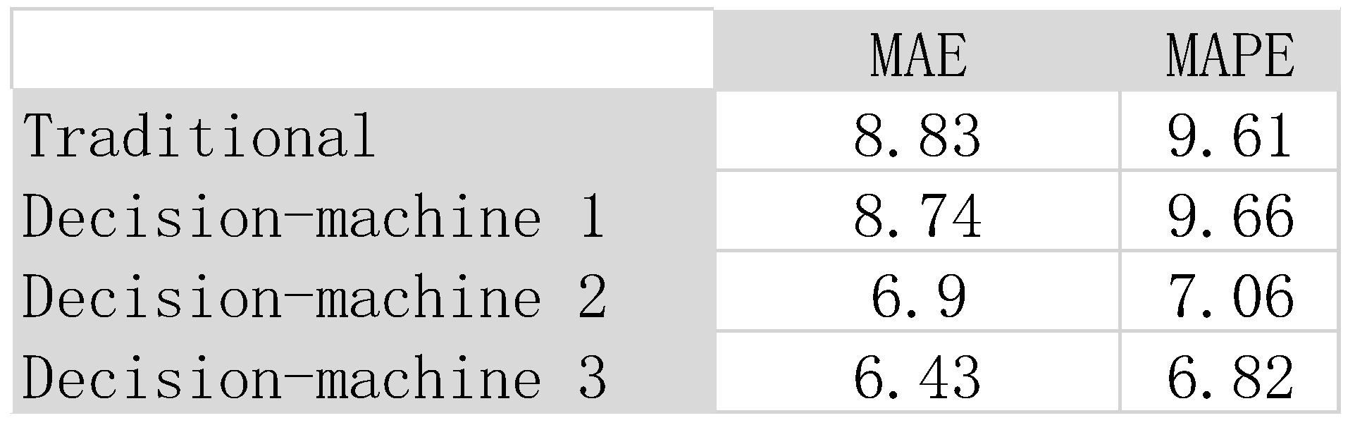
Table 3 shows the MAE and MAPE metrics of traditional methodologies and the decision-machine’s three predictions.

The average MAE and MAPE of the three decision-machine’s predictions is 7.35 and 7.84 respectively, which are both better than traditional methodology’s MAE of 8.83 and MAPE of 9.61.

The data in Table III shows that the decision-machine performs better than traditional methodologies; the MAE of the decision-machine’s second (6.90) and third (6.43) predictions were much better than the traditional methodology’s MAE of 8.83; the first prediction was slightly better than traditional methods; the MAPE of the decision-machine’s predictions, the second and third were much better, while the first one was almost the same as traditional method’s MAPE.

Under uncertain circumstances that have significant volatility and fluctuations, such as the random movement of pollen or an electron, traditional methods cannot produce a trajectory but can only produce a probability of where the position may be. As seen from Table II, the traditional methodologies can only produce an average line of 106; the decision-machine can produce three trajectories (Figure 2) for all three predictions produced with better MAE and MAPE shown in Table III; two predictions were better than traditional methods, with one being close to the actual results. The decision-machine is able to produce consistent and reliable predictions but can’t assure 100% accuracy, though is more accurate than traditional methods; the decision-machine is able to give a trajectory of the data and not just an average or vague probability of where the future data points might be, which shows the efficiency and effectiveness of the decision-machine is quite high.

IV. DISCUSSION

Scientists have always sought to answer a question of: how do we acquire definite knowledge of mother nature?

The modern-day scientific community firmly believes that there is some eventual terminal structure of mother nature that is just waiting for us to find it, and this structure can be simply described by mathematical language. Based on deduction and induction, the scientific community believes that scientific discovery is to discover nature’s secrets by using the entity – property – structure approach (conceptual framework + differential equations + integral solution –> function –> output a numerical value).

There are two unavoidable difficulties when it comes to scientific discovery by simply using deduction and induction, which are:

1): The irreversibility of the arrow of time: the future cannot simply be deduced from the past, i.e. the unpredictability of the future.
2): The overall complexity (1 + 1 > : the collective whole cannot be induced from part, the collective whole does not solely consist of independent parts, the individual parts themselves are intertwined with complex relationships, i.e. one cannot simply induce whole from part.

In other words, deduction and induction won’t only be able to ensure that a prediction will be effective (from past to future, from part to whole). Hume realized the limits of human cognitive understanding (Hume Problem), i.e. not being able to accurately predict the future just based on the past, as well as not being able to accurately predict the unknown from the known. Hume pointed out that humans mostly rely on observation and experience to discover the laws of nature, especially relying on the habits that have formed in the mind due to the constant observation of nature's continually repeated events (the sun rising every day, etc...). The experience gained through observation of what Hume said, especially those events that happen over and over, which in a sense is just “information”, i.e. how do we understand more about nature by performing effective operations (the habits that have formed in our minds) through acquiring the most effective information (nature’s repetitive events) from observation data.

The question then naturally arises: could we construct a machine to conduct scientific discovery by forming "habits" of nature's repetitive patterns from the observed data?

Richard Feynman pointed out that we can’t rely on machines to discover laws of nature, i.e. a machine won't be able to blindly find a "satisficing" hypothesis because a machine cannot reason in absence of a standard evaluation criteria to guide it. This leads us to the problem of how effective scientific discovery can be, i.e. how to evaluate the effectiveness of each proposed hypothesis?

In this paper we propose a way to unify the deduction and induction, make induction follow rules to reason just like how deduction does, all together the goal is to be able to ensure effective reasoning (event – information – operation –> matrix –> output a vector as operation). The induction rules that we have proposed are 1) similarity degree 2) effective operational level 3) consistency, and in this way we can construct a decision-machine to conduct effective scientific discovery based on inductive rules.

The specific steps of when the decision-machine conducts scientific discovery are:

1): The decision-machine randomly generates a set of “hypotheses”;
2): The decision-machine calculates the similarity degree of each generated hypothesis with mother nature;
3): The decision-machine adapts to mother nature by continually self-learning and self-adapting;
4): The decision-machine outputs an effective operation with maximum similarity degree by evolution;
5): The decision-machine simulates (reconstruct the past and predict the future) nature’s behavior with the outputted effective operation;
6): The decision machine, through steps 1-5 obtains a satisficing hypothesis by recursive learning;

By utilizing the inductive rules to consistently reason, the decision-machine goes from not knowing anything about nature at all to gradually obtain a hypothesis that most approximately conforms to nature’s behavior by the experience of gains and losses.

When compared to human observers conducting scientific discovery, the decision-machine’s approach to scientific discovery has three advantages:

1): Objectivity: The decision-machine obtains effective information (maximum similarity degree) from the observed data, then "forms" habits (effective operation) solely based on the said information obtained, and by doing so in this way subtly avoids the prejudices, emotions, and likes/dislikes of human scientists when conducting scientific discovery.
2): Effectiveness: By relying on the same induction rules (similarity degree, effective operational level, and consistency) the decision-machine avoids "debating" the incommensurability of scientific hypothesis like human scientists, which leads the decision-machine to reasonably conduct scientific discovery without any "controversy" and "distractions".
3): Automation: The decision-machine can automatically “find” satisfactory hypothesizes from observed data 24 x 7 by self-learning, and self-adapting.

Unfortunately, scientists cannot construct a “theory of everything” to exhaust all the possibilities of nature, especially when nature itself may be creatively evolving. At the same time, we are not attempting to create a fully perfect omnipotent machine to accurately predict the future (no else can either), but rather a self-learning, self-adapting machine that can cope with the problems that even the machine designer cannot foresee, to “deal with” nature’s infinite possibilities. Scientific discovery isn’t just about backtracking the past and to predict the future but more importantly it’s about challenging the uncertain, ever-changing, modifiable nature. We cannot naively believe that nature is static and there is some simple final structure “sitting” somewhere for us to find, scientific discovery is more about finding the unknown of the unknown (nature’s “ignorance”). We have proposed integrating both the principle of quantum superposition and evolutionary algorithm: first utilize superposition to generate many possible hypotheses to simulate nature’s many possibilities, then by utilizing the survival of the fittest principle to evolve a hypothesis that most approximately conforms to nature, and finally through means of recursive learning the decision-machine dynamically “deals with” the unknown of the unknown.

V. CONCLUSIONS

In this paper we constructed a decision-machine to conduct scientific discovery. Three induction rules were defined to ensure the effectiveness of inductive reasoning. The randomness trajectory of the entity is simulated by a computer program. The decision-machine simulated the trajectory of the entity with 0.86 similarity degree, and predicted the future trajectory of the entity with 7.84% MAPE; the decision-machine’s predictions performed better than the “best” traditional methods (mean value way), which were 9.61% MAPE. Basically, from a geometrical perspective, the decision-machine is able to reconstruct any curve and probabilistically predict that curve's future movement by using a self-adapting program to optimize an operation matrix that's constructed from eight basic “quantum logic gates"; we can see this as an analogy to Descartes attempt of analytic geometry to use algebra to describe the geometric curve; by utilizing a self-adapting program to describe the geometric curve, we can "name" it "programming geometry".

If mother nature truly “plays dice” with the universe, then the decision-machine approach may fare better than traditional methodologies. We don’t know which one nature will “chose” as the real world from the many possible worlds, or maybe nature doesn’t know either, nature is never finished, “she” is constantly creatively evolving.

We know that nature plays dice with the universe. Nature knows that we know that nature plays dice with the universe. We know that nature knows that we know that nature plays dice with the universe. Yet nature still plays dice with the universe. So instead of asking does nature play dice with the universe, why don’t we just let the decision-machine play dice with nature?

Acknowledgments

This work received no funding.

Conflicts of Interest

The authors declare that they have no conflicts of interest regarding the publication of this paper.

References

Popper, K. R., & Freed, J. (1959). The logic of Scientific Discovery: Karl R. popper. Hutchinson.
Strevens, M. (2022). The knowledge machine: How an unreasonable idea created modern science. Penguin Books.
Kuhn, T. S. (1973). The structure of Scientific Revolutions Thomas S. Kuhn. Univ. of Chicago Press.
Mach, E. (2019). Science of Mechanics: A Critical and historical account of its development. Forgotten Books.
Whitehead, A. N. (1957). The concept of nature. University of Michigan Press.
Strogatz, S. (2020). Infinite powers: How calculus reveals the secrets of the universe. Houghton Mifflin Harcourt.
Einstein, A. (1905) On the Movement of Small Particles Suspended in Stationary Liquids Required by the Molecular-Kinetic Theory of Heat. Annalen der Physik, 17, 549-560. (Reproduced in Stachel, J. (1989) The Collected Papers of Albert Einstein. Vol. 2, The Swiss Years Writings, 1900-1909, 223-236.).
Feynman, R. P., & Hibbs, A. R. (1965). Quantum Mechanics and path integrals. McGraw-Hill Publishing Co.
Feynman, Richard Phillips. (1967). The character of physical law. MIT. Press.
Trimmer, John D. "The Present Situation in Quantum Mechanics: A Translation of Schrödinger's 'Cat Paradox' Paper." Proceedings of the American Philosophical Society 124, no. 5 (1980): 323–38.
Whitehead, A. N. (1929). Process and reality.
Wittgenstein, L., & Hacker, P. M. S. (2016). Philosophical investigations. Wiley-Blackwell.
Wittgenstein, L., & Georgallides, A. (2016). Tractatus logico - philosophicus. Ekdóseis Íambos.
Hume, D. (1985). A treatise of human nature (E. C. Mossner, Ed.). Penguin Classics.
David Hume, E. S. (2023). Enquiry concerning human understanding.
Von Neumann, J.; Morgenstern, O. Theory of Games and Economic Behavior; Princeton University Press: Princeton, NJ, USA, 1944.
Heisenberg, W., the Physical Principles of the Quantum Theory, Chicago, IL: The University of Chicago Press (1930).
Dirac, P.A.M., the Principles of Quantum Mechanics, Oxford University Press (1958).
Von Neumann, J. Mathematical Foundations of Quantum Theory, Princeton, NJ: Princeton University Press (1932).
Devlin, K. J. (2010). The unfinished game: Pascal, Fermat, and the seventeenth-century letter that made the World Modern. Basic Books.
Savage, L.J.: The foundation of Statistics. Dover Publication Inc., New York (1954).
Darwin, C. (2011). The origin of species. William Collins.
Holland, J., Adaptation in Natural and Artificial System, Ann Arbor, MI: University of Michigan Press (1975).
Goldberg, D.E., Genetic algorithms – in search, optimization and machine learning, New York, NY: Addison-Wesley Publishing Company, Inc. (1989).
Koza, J.R., Genetic programming, on the programming of computers by means of natural selection, Cambridge, MA: MIT Press (1992).
Koza, J.R., Genetic programming II, automatic discovery of reusable programs, Cambridge, MA: MIT Press (1994).
Xin, L., Xin, H. Decision-making under uncertainty – a quantum value operator approach. Int J Theor Phys 62, 48, (2023). [CrossRef]
Xin, L.; Xin, K.; Xin, H. 2023 On Laws of Thought—A Quantum-like Machine Learning Approach. Entropy, 25, 1213. (doi:10.3390/e25081213).
Xin, L. Z., & Xin, K. (2025). Is the Market Truly in a Random Walk? Searching for the Efficient Market Hypothesis with an AI Assistant Economist. Theoretical Economics Letters, 15, 895-903. [CrossRef]

Figure 1. Fitting results of the training data produced by the decision-machine, the blue line is the entity’s position and the yellow line is the position calculated by the decision-machine.

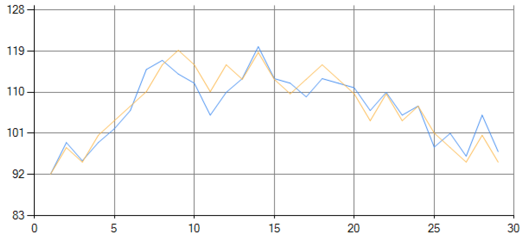
Figure 2. The three predictions (a)-(c) of the verify results produced by the decision-machine, the blue line is the entity’s position, the yellow line is the predicted position by the decision-machine, and the red line is the average of 1000 predictions made by the decision-machine which is to simulate traditional methods mean value way.

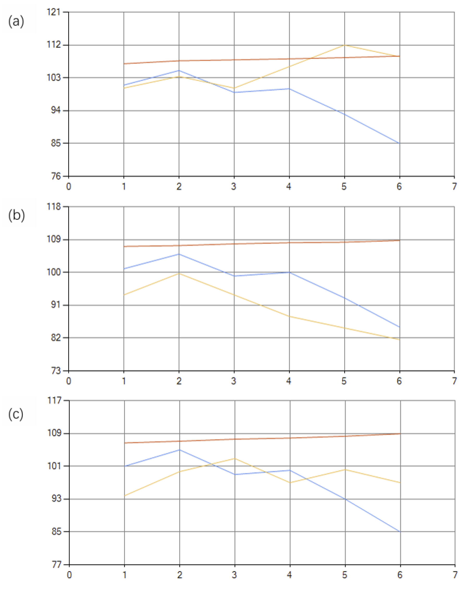
Table 1. represents that the entity moved downwards along the curve of the graph; the third column is the position of the entity; the fourth column is the decision made by the decision-machine, where 0 represents the decision-machine believes that the entity will move upwards along the curve of the graph and 1 represents the decision-machine believes that the entity will move downwards along the curve of the graph; the fifth column represents how confident the decision-machine is when taking actions (degree of beliefs); the sixth column is the calculated position of the entity by the decision-machine.

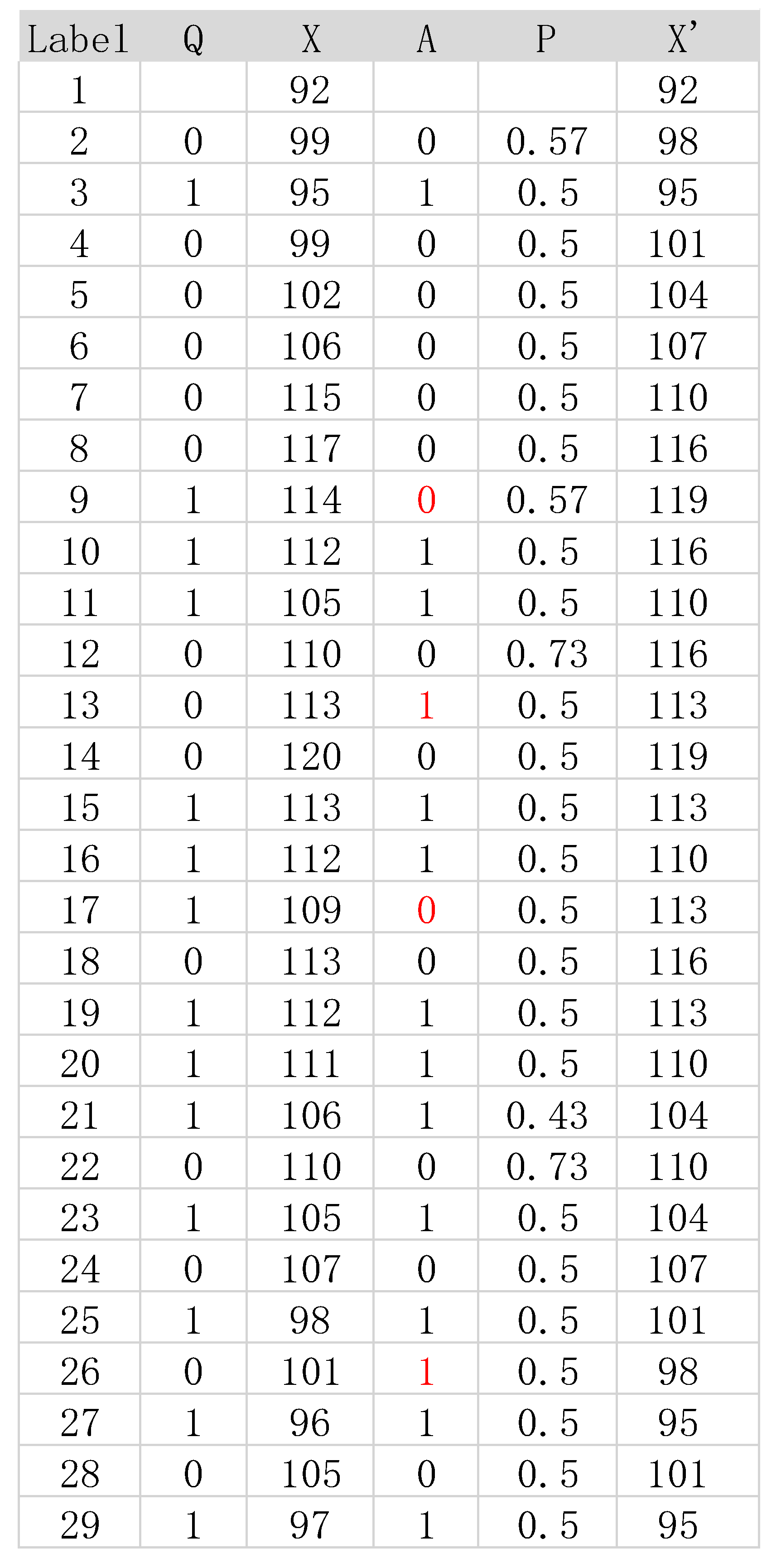
Table 2. Results of the verify dataset. The first column is the label of the verify data; the second column is the position of the entity; the third column are the traditional methodologies predictions; columns four through six, DM1-DM3 are the three decision-machine’s predictions.

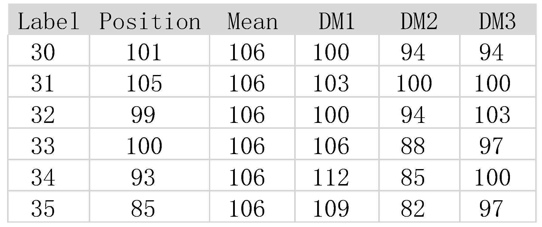
Table 3. RMAE and MAPE metrics of traditional methodologies and three decision-machine predictions.

Disclaimer/Publisher’s Note: The statements, opinions and data contained in all publications are solely those of the individual author(s) and contributor(s) and not of MDPI and/or the editor(s). MDPI and/or the editor(s) disclaim responsibility for any injury to people or property resulting from any ideas, methods, instructions or products referred to in the content.

© 2025 by the authors. Licensee MDPI, Basel, Switzerland. This article is an open access article distributed under the terms and conditions of the Creative Commons Attribution (CC BY) license (http://creativecommons.org/licenses/by/4.0/).

Copyright: This open access article is published under a Creative Commons CC BY 4.0 license, which permit the free download, distribution, and reuse, provided that the author and preprint are cited in any reuse.

On Scientific Discovery–A Decision-Machine Approach

Abstract

Keywords:

Subject:

I. INTRODUCTION

II. METHODS

III. RESULTS

IV. DISCUSSION

V. CONCLUSIONS

Acknowledgments

Conflicts of Interest

References

MDPI Initiatives

Important Links

Subscribe