Submitted:
15 September 2025
Posted:
16 September 2025
Read the latest preprint version here
Abstract
Among the predictions of the standard model of cosmology, known as ΛCDM, a number contradict observations. These are referred to as problems (those of dark matter, dark energy, etc.) or tensions (the Hubble tension, the S8 tension, etc.). We only know in total about 5% of the matter and energy in the universe. These problems are currently examined separately from one another, each on its own. In this paper, we examine a discordant hypothesis: all these problems are symptoms of a single problem, that of a miscalculation of the speed of light on a cosmological scale. We propose that it be lowered by a factor of about 2.4 compared to its value in the local vacuum (solar system). Our model requires no new matter nor new laws; based on general relativity (Schwarzschild metric, extended Shapiro effect), it allows predictions to be made that can be compared with observations. For the ten or so problems discussed, the comparison is favorable, including from a quantitative point of view. Its validity is reinforced by the simplicity and uniqueness of the perspective taken on different physical situations. Should we advocate a paradigm shift and abandon the standard model (which appears to have been refuted)? This model continues to explain a great many facts. At this stage, we argue for further exploration of our hypothesis and detailed examination of the various difficult cases, in coexistence with the standard model, whose interpretation needs to be renewed.
Keywords:
dark matter
; dark energy
; impossible galaxies
; Hubble tension
; S8 tension
; temporal variation of the cosmological constant
; cosmological constant and vacuum energy
; extended Shapiro effect
; general relativity
; cosmology
; equivalent refractive index
; Schwarzschild metric
Introduction
When reviewing contemporary cosmological literature, it is clear that researchers are concerned about a number of issues. These are referred to in various ways: problems, tensions, questions, etc. Some even speak of a crisis. Several difficulties appear to be significant and persistent, threatening the standard model. Others, encountered occasionally, seem secondary: we expect to overcome them with more data. We can cite (the following list is neither exhaustive nor ranked): the problem of dark matter, the problem of dark energy, the problem of the variation of the cosmological constant over time, the Hubble tension, the S8 tension, impossible galaxies, the mysteries of inflation, the problem of the cosmological constant and vacuum energy, the relative absence of dark matter in the Milky Way, understanding the multiverse, etc. In total, we are told that we only know 5% of the matter and energy in the universe.
These topics are treated individually: the authors do not consider that they may be symptoms of the same “problem.” In this article, on the contrary, we will ask ourselves whether there is a single cause for all these problems. The thesis we seek to establish is as follows: on a cosmological scale, the speed of light is not equal to its value c0 in a vacuum (that in the solar system, for example), but to a smaller value cc (index c as cosmological), explainable by an effect of general relativity (extended Shapiro effect). The reduction factor nc = c0/cc could be of the order of 2.4; this is the value that allows us to accommodate, on average, the apparent existence of dark matter and dark energy, as well as the resolution of the other difficulties mentioned.
Our plan will be as follows. In the first part, we will discuss our calculation of an equivalent refractive index nc on a cosmological scale. We will then (in the second part) review the various problems mentioned and examine how our hypothesis can alleviate them. In the third part, we will discuss the areas where our proposal does not work satisfactorily. While it works on average, it does not explain all specific cases: what avenues should be explored? We will also propose an epistemological discussion on the place of our proposal in relation to the standard model. We will conclude with a few concluding remarks.
Here we offer a general overview of our research. To be convincing, each point raised deserves to be treated separately and in depth. Our angle of attack is a different one : given the multitude of diverse “tensions,” the prospect of providing a single solution to them has a particular strength. This can only be said if we maintain a certain distance from the whole, without dwelling on each point (at the risk of an apparent lack of rigor). All of this should be understood as a research program, requiring as many individual in-depth studies. In this context, the bibliography will remain succinct: the issues are regularly raised in the public arena, in articles and popular magazines. Numerous references can be found in Guy (2022, 2024a); we add a few that are missing. Some passages from our works are reproduced here with modifications.
1. A Refraction of the Universe on a Cosmological Scale
1.1. Calculation of an Equivalent Refractive Index
We have mentioned a lower speed of light on a cosmological scale. Let’s see how this is possible. We can consider the Shapiro effect, understood by general relativity: it already shows us, for the influence of a single object, the slowing down of the speed of light. The time delay can be interpreted as a lower speed, insofar as the distances evaluated are Euclidean distances projected onto distant objects (use of standard candles, variation in the angular sizes of objects, etc.), whereas the actual path of light, which follows the detours of a non-Euclidean space (the Shapiro effect is an effect of general relativity), is longer than the “direct” path. From this, we can already assert that c is certainly not equal to c0 on the scale of the universe. The question is: can the Shapiro effect be extended to all objects in the universe?
To do this, we can use the Schwarzschild metric, which is also used to predict the aforementioned effect. It is not used for an expanding universe, but has the advantage of having “balanced” coefficients for space and time, unlike the FLRW (Friedmann-Lemaître-Robertson-Walker) metric, which gives the spatial coefficient a privileged role. Let’s take this as a first approach. Let’s place ourselves in the middle of a universe filled with masses of various sizes, from dust and gas to clusters of galaxies, including stars and galaxies. We do not know the details of this distribution, so we can replace it with an average density ρU, that of the universe, to be integrated over a universe of equivalent gravitational radius RU (spherical symmetry). In this respect, we agree with authors who frequently refer to an average density of the universe, as well as an equivalent gravitational radius, despite expansion. The notation ds2 = 0 expresses the propagation of light in general relativity. From this we obtain dr2/dt2, which allows us to derive an equivalent index. By performing the indicated summation, we derive the formula (Guy, 2024a):
For the equivalent index on a cosmological scale, where G is the gravitational constant, c is the speed c0, ρU is the average density of the universe, and RU is its equivalent gravitational radius. We have not found any calculations of this type in the literature, where we only read for nc a first-order expansion for the local effect of point masses.
The question then is whether an index of 2.4 is conceivable. In the diagram in Figure 1 from Guy (2024a), we have plotted, in logarithmic coordinates, straight lines of iso-values of the index, as a function of the size of the universe on the x-axis and the average density on the y-axis. This is a representation of the following formula, derived from the value of the index (1):
In Figure 1, the highlighted areas correspond to possible gravitational radii, ranging from 10 to 100 billion light-years, as well as density ranges corresponding to what is currently estimated, between 10-26 and 10-28 kg/m3, and for a band of indices between 1.2 and infinity, with the index line 2.4 indicated.
One might have expected the three bands to be independent of each other. But, remarkably, the index line 2.4 fits perfectly into the intersection zone of the two bands of densities and sizes of the universe that are reasonable in relation to what we know.
Thus, our initial approach shows that it makes perfect sense to consider a speed of light on a cosmological scale, which we denote cc, reduced by a factor of 2.4 compared to the speed in a vacuum. One might say that this is a significant reduction, but let’s not forget the scale of the problem we are facing, with 95% of the matter and energy in the universe unknown. We need a solution that is up to the task, and we have not forced anything.
1.2. How Can We Understand the Speeds of Celestial Bodies?
The problems listed in the introduction are primarily problems of velocity (they appear too high), not of mass or energy. The speeds of distant celestial bodies are estimated using v/c ratios (Doppler effect). If c is smaller on a cosmological scale, then, for an equal v/c ratio (the ratio provided by the measurement, which we must respect), v will naturally be smaller. We then no longer need to increase v to accommodate dark matter. More generally, all velocities are defined in velocity ratios (see the relational epistemology that we promote, Guy, 2024b), and that of light is no exception. Any speed on our scale implicitly incorporates a quantity c0 in the definitions of lengths and times. This relational spirit gave us the motivation and courage to vary c, but from a formalistic point of view, we could have done without this philosophical detour.
For our galaxy, the velocities of objects are evaluated, for a significant fraction, by the parallax method, and we use the value of the standard speed of light, i.e., c0 (and not cc). There is no special correction to be made (in accordance with the deficiency of dark matter in our galaxy compared to other galaxies, see the section below). Let’s clarify the relationships between velocities and masses: we need them to estimate the amount of dark matter. These are given by the virial theorem (equality between kinetic energy and potential energy for systems with a certain degree of stationarity): all other things being equal, for two systems 1 and 2, we observe an equality between the ratio of masses and the ratio of velocities squared, i.e.,
Let’s clarify the notation. Let’s call v’m’, or v “measured,” the speed that we evaluate using standard methods (we put the index m in quotation marks); to evaluate it, we have placed the value c0 of the speed of light in a vacuum in the denominator of the ratio v/c (our measurement), without questioning it. But it turns out that the so-called measured value v is too large compared to ve (v subscript e) estimated from known masses. By putting another, smaller speed of light, cc, in the denominator of the ratio v/c, for c on a cosmological scale, we can lower v and return to the estimated value without adding invisible mass. We define a ratio α between the two speeds, v’m’ / ve, or c0 / cc : it acts as an equivalent refractive index, similar to the one we have noted as nc. Relation (3) shows us that for a speed ratio of 2.4 between two speed estimates, the ratio of the masses to be attached to them will be of the order of 6, or (2.4)2.
2. Examination of Problems
2.1. Dark Matter
Let’s see what these considerations tell us about dark matter. It is interesting to note that the ratio announced by the authors between baryonic matter (i.e., ordinary matter) and dark matter is roughly constant and close to 6 for a wide variety of situations. This ratio results from a velocity ratio equal to the square root of 6, or close to 2.4, which is what we started with. Let’s try to find it in different examples.
Among the many places where dark matter is discussed, let’s look at the emblematic example of spiral galaxy rotations. Figure 2 shows a few curves (taken from the work of Mc Gaugh, 2014; McGaugh et al. 2016; reproduced in Guy, 2024a), where velocity is represented on the y-axis and distance from the center of the galaxy on the x-axis. For those examples where they are available, the measured value is represented by dotted lines and the estimated value by solid lines. The authors have placed great emphasis on the plateau of measured velocities of galaxies at great distances from the center. In reality, the curve eventually descends; what is intriguing is the difference between the measured value and the estimated value. For a number of galaxies, we see that this difference is not only apparent on the plateau, but throughout the entire curve, including the increase in velocities near the center. For a number of galaxies, the ratio is 2.4! This is what will provide the ratio between baryonic matter and dark matter of around 6, as announced.
We are obviously not saying that all galaxy profiles are of this type. It is more complicated than that, but for us it is a crucial starting point for this issue: it does not seem to have been discussed in the literature. This observation rules out the MOND theory, which is limited to low accelerations, whereas the problem already arises for high accelerations near the center of galaxies. This observation also seriously questions the hypothesis of dark matter halos postulated to explain the plateaus, without looking at what is happening at the center.
Dark matter is considered in many other places, particularly historically, in galaxy clusters. We will not go into a detailed discussion of how it is detected in clusters. We will simply note that there is still a postulated missing mass of about 6 times the “visible” mass.
Gravitational Lenses
The previous recipe also works for gravitational lenses: this is remarkable, given that the formalism used to detect dark matter is different. Let us return to the generic formula giving the angle of deviation of the light ray θ caused by the influence of an intervening mass M, passing at a distance d from this mass. It is written as:
Where G is the gravitational constant and c is the speed of light. The angle involves a ratio M/c2. By dividing c by 2.4 and keeping the angle, or the ratio, equal (this is the measurement), we divide the mass M by 6. There is no need to add dark matter. The authors proclaim that this is proof of the existence of dark matter. It can also be seen as renewed encouragement for our hypothesis, for a different invoked process.
Dark Matter and Cosmic Microwave Background
The CMB (cosmic microwave background) is the remnant of radiation emitted by the hot, dense horizon during the early stages of the universe. It refers to the moment when photons can escape and the universe becomes transparent. The horizon is the opaque wall we encounter when we go back in time, reaching a state of the universe that did not allow light to pass through (estimated at 380,000 years after the Big Bang). Originally, this radiation had a temperature of around 3,000 K, but the expansion of the universe has brought it down to around 3 K today. CMB radiation is that of a black body, meaning that the spectrum of emitted wavelengths is solely a function of temperature. We measure very small temperature fluctuations (determined by the wavelengths of light in the context of black body radiation) of the order of 10-5. The Planck satellite has made it possible to map these fluctuations. They are linked to fluctuations in the density of the medium emitting the CMB, via the propagation of acoustic waves in the dense plasma of this medium. The relationship between temperature and density fluctuations has been demonstrated (Aubert, 2019):
The δT/T ratio is the fundamental starting point for various developments on the CMB. As measurements lead us, we are drawn towards an excessive density ratio compared to what is expected for ordinary matter alone, and this is where dark matter comes in.
The CMB horizon from which the 3K radiation originates is moving away from the observer due to the expansion of the universe. To map the temperatures, we must take into account the escape velocity, deduced from the Doppler effect (for a z of around 1100). If our reasoning is correct, we can imagine that the escape velocity has been exaggerated; this velocity shifts everything towards the red, i.e., it lowers the temperatures T of black bodies. On the other hand, the δT remain the same (these are differences, the two limits of the interval are shifted equally by the expansion). Thus, for the same red shift, by decreasing the escape velocity, which would have been exaggerated, we increase the thermal red shift, i.e., we decrease the temperature. We increase the ratio δT / T; relation (5) shows us that we then increase the absolute value of the density fluctuation. Thus, as a first approximation, we would not need additional dark matter for the CMB either.
2.2. Dark Energy
Carried by our momentum, let’s look at dark energy. This is evidenced by an acceleration in the expansion of the universe. On this subject, we trust the astrophysicists who tell us that adding a cosmological constant to Einstein’s equations accounts for the acceleration. So let’s rewrite these equations with the constant Λ, we have:
Where gμν is the metric tensor, Rμν is the curvature tensor, and Tμν is the energy-momentum tensor, where μ and ν denote space and time coordinates. We note the intervention of c to the power of 4. If we estimate that the correct value is c / 2.4 and that the term in Λ is useless, a correction is necessary to be applied to the energy momentum tensor with a factor c4 - 1. Here it is approximately equal to 35. In terms of mass energy, or mass density, this leads us to a ratio between dark energy and energy associated with known matter, corresponding to that announced by astrophysicists (freeing us from dark matter; see the calculations in Guy, 2024a).
In short, dark matter and dark energy are the names given to the corrections made to accommodate the error of taking c = c0 for the speed of light on a cosmological scale. The consistency of these different results is a testament to the remarkable work of astrophysicists.
2.3. Impossible Galaxies and Models of the Universe
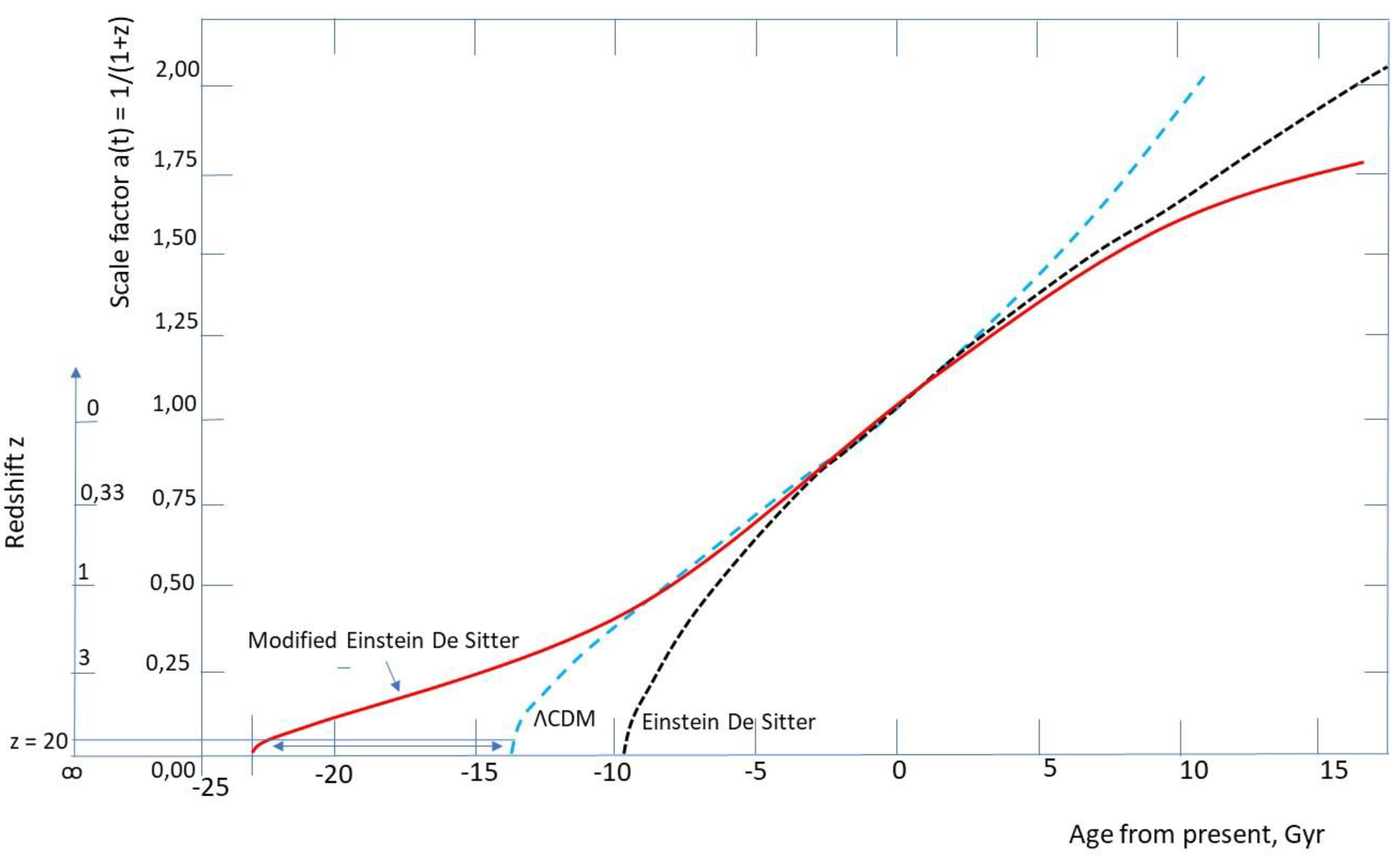
Let us now look at the history of the expansion of the universe. We must begin by inclining Hubble’s diagram (which links velocities and distances) and proposing a value of H0 (the value of the Hubble constant) divided by 2.4. In our initial approach, we will not go into detail about the equations of the universe models that describe the variation of the scale factor a as a function of cosmic time; they take into account both the values of the densities Ωi of the different energy components and the Hubble constant. An Einstein de Sitter model (with no dark matter nor dark energy), modified by a new value for the Hubble constant, gives an initial idea of what is happening. We presented it in Guy (2024a) and reproduce it in Figure 3. We have also represented the standard ΛCDM model and the unmodified Einstein de Sitter model.
The age of the universe is increased: Einstein’s modified de Sitter model gives an age of 25 billion years. Taking the inverse of the modified Hubble constant gives an age of 33 billion years. What is notable is that the differences between the standard model and the modified Einstein de Sitter model are significant for the early stages after the Big Bang, as well as for the most recent periods (the two models coincide for the middle part, but not at the beginning nor the end). With regard to the earliest ages, we can mention the problem of impossible galaxies. These are galaxies observed (in infrared by the James Webb Space Telescope) that appear to be very young compared to the time of the Big Bang (a few hundred million years later) but which are already structured like mature galaxies that, according to standard models of galaxy formation and evolution, should be over a billion years old (massive black holes encountered at these times are also surprising, according to the authors). According to the modified Einstein de Sitter model, we see that galaxies observed at high redshift have had plenty of time to form, without resorting to mechanisms that are different from those calibrated for closer galaxies.
The discrepancy between the modified Einstein de Sitter model and the standard model is also significant in recent periods. Results recently announced by astrophysicists (DESI collaboration) provide a field of research for discussing the discrepancies between observations on the evolution of the universe and the standard model. Will they support the view (as we might) that it is not necessary to propose new hypotheses to explain certain features of recent evolution?
2.4. The Variation of the Cosmological Constant over Time
In our understanding, the cosmological constant mimics a way of using Einstein’s equations with a speed of light that is lower by a factor nc on the cosmological scale than its “usual” value in a vacuum c0 . The factor nc depends on the average density and the equivalent gravitational radius of the universe. Taking into account the expansion of the universe, we can impose a constraint of a decrease in density and an increase in the equivalent gravitational radius, with a constant amount of matter, according to
where M is the mass of the universe. In formula (1) giving nc, ρ and R appear in the factor ρR2. We derive from (7) that
Which we can insert into the equation for nc:
Looking back in time, we see that as the radius of the universe decreases, the index nc increases. In the context of the equivalence between the cosmological constant approach and the apparent refractive index nc approach, we showed in Guy (2024a) a relationship between the density associated with dark energy, that associated with ordinary mass, the cosmological constant, and the index, given by:
From this we derive a value for the cosmological constant
where we have used relation (7). We can thus see the dependence of Λ on the radius of the universe R, for a universe with a total mass equal to M. The cosmological constant, another name for a correction calibrated by the speed of light on a cosmological scale, can therefore vary over time, and we can expect it to be greater in the past when the universe was smaller and denser. Can this be reconciled with the results of the DESI collaboration?
2.5. The Cosmological Constant and Vacuum Energy
Much research is being conducted to understand what lies behind dark energy, with a density denoted Ωv or ΩΛ. As we have just seen, many authors link it to the cosmological constant Λ. The latter, which opposes the force of gravitational attraction, was introduced by A. Einstein into his equations in order to guarantee a stationary universe. Others see it as an expression of vacuum energy (in the quantum mechanical sense): however, according to particle physics and quantum field theory, there is a large difference in order of magnitude between the two energies. The vacuum energy estimated by quantum mechanics is about 1040 times greater than the energy associated with the cosmological constant, which makes the supposed link between the two problematic. For some authors, this is one of the greatest enigmas in physics. For us, the cosmological constant poses no problem, insofar as it does not refer to a real force of nature, but expresses the correction of an initial misunderstanding. The problem of the huge gap between the vacuum energy determined by quantum mechanics and the cosmological constant does not arise.
2.6. Hubble’s Tension
Hubble tension expresses the discrepancy between the two main estimates of the Hubble constant H0: - that obtained from observations of the local universe (galaxies close to the scale of the universe): distances are estimated using standard candles (in particular Cepheid variables), velocities using the Doppler effect; and - that obtained from studying the cosmic microwave background (CMB). In the first case, we obtain a value of 73 km/s/Mpc. And in the second case, a value of 67.7 km/s/Mpc. The two areas of uncertainty do not overlap, hence the word “tension.” What can we say? First, by dividing the two values by 2.4, as we suggested above, we bring them closer together. This is done without changing the values of the uncertainties, which depend on the measurement conditions in the broad sense. The confidence intervals then converge. We can say more. In the first case, the measurement is, in a sense, direct. In the second, it is model-dependent. In fact, we then look at how the sizes of the CMB fluctuations are distorted by the expansion of the universe governed by the standard model. The constant H0 is involved, and the method for evaluating it consists of studying which value of the constant accounts for the observed results. It turns out that the standard model contains dark matter and dark energy, which we want to do without. So if we modify the parameters of the standard model, with equal CMB measurements, we will modify the value of the Hubble constant derived from its observation. According to the authors, simply decreasing the fraction Ωm (ordinary matter in the absence of dark matter) increases the value of H0.This is therefore a second avenue offered by our approach (the literature shows many) to relieve the Hubble tension, to be clarified by revisiting the standard model in greater depth.
2.7. The S8 Tension
We refer to the S8 tension in relation to the parameter of the same name (also denoted σ8 and the Σ8 tension), which describes the inhomogeneity of the distribution of matter in the universe. To define this parameter, we place ourselves inside a sphere with radius h-1. 8 Mpc, where h = H0/100 (S8: S for standard deviation σ, or Σ, 8 for the radius of 8 megaparsecs). There is tension because there is a discrepancy between observations and models (which are constructed in particular from the CMB). These predict greater heterogeneity than is observed. Our approach allows us to move towards reducing this tension. Indeed, if we divide H0 by 2.4, we increase the size of the sphere on which the parameter is constructed, so we do not predict as much heterogeneity. In this reasoning, we do not have to change the observations inserted into a model of space projected from our local one.
2.8. The Relative Poverty of Our Galaxy in Dark Matter
It is interesting to note that, for our Milky Way, the assumed amount of dark matter is significantly less than in other galaxies of the same type: instead of being six times greater, it is only twice as great (Jiao et al., 2023); that is, one-third of the usual ratio. We see a link here with the fact that, in the case of our galaxy, the velocities of stars are largely measured by parallax effects. We had anticipated, in the form of a question (Guy, 2022), that dark matter would then not need to be postulated. Let’s try to clarify this: let’s look at the proportion of velocities measured by parallax compared to those measured by the Doppler effect. Jiao et al. (op. cit.) indicate that the 1.8 billion stars surveyed by the Gaia satellite were measured for both parallax velocities and radial velocities by the Doppler effect. Roughly speaking, one-third of the velocity is measured by the Doppler effect in our galaxy, while for distant galaxies, the velocity is measured by the Doppler effect alone. If we estimate that, statistically, each component of velocity is responsible for one-third of the dark matter effect, this corresponds to the announced proportion. This could therefore be consistent with our proposal...
2.9. The Mysteries of Inflation
When studying the very beginnings of the evolution of the universe, various problems arise, in particular that of its homogeneity (how can causally distant regions be so similar?) and its flatness. It was to resolve these problems that the mechanism of inflation was proposed: an expansion of the universe by a factor of 1050 in a time of the order of 10-32 s! How is this possible? This excessive expansion of space and this very short duration bring us back to the meaning of space and time. We need to reconsider them, in the sense that neither one nor the other exists. As we have shown in our work, within the framework of relational epistemology (see, for example, Guy, 2011, 2019, 2024b), we are only faced with movements to be compared with each other. From this we derive the concepts of space and time (subject to choices and limitations to be specified). The value of an optical index is a way of comparing two speeds of light (these refer to the particular movement chosen as a standard, from which the standards of space and time are derived). At the beginning of the universe, matter was very dense with a speed of light cc much lower than c0, which guided the unfolding and measurement of physical processes. This made it possible to define standards of space and time that were completely different from those based on c0. If we now return to our usual standards, it is like “playing the film” at speed c0, so that the variation in time becomes infinitesimal and that in space becomes excessive (see Guy, 2022).
2.10. Captive Light (Black Holes, Universes)
The previous view can be applied to the way we talk about the speed of light in black holes. We continue to talk about c0 locally, but if we take a step back, we can say that when we try to cross the event horizon outward, it is as if the speed of light could be canceled out (seen from the outside, it is not equal to c0). If we return to the optical comparison, we can calculate an optical index for the Schwarzschild black hole. For this metric, the index is:
For the value of the horizon radius r = 2GM/c2, we have an asymptote with n tending to infinity; the speed of light tends to zero.
For the universe as a whole, we find the same situation for straight lines in the plane (Ru, ρu) along which nc is infinite (Figure 1). The universe then prevents the progression of light on its megascopic scale (whereas locally, it is still equal to c0). With
nc is infinite for ρu Ru2 = c2 /4πG. This leads us to a discussion of the “horizon,” which should be distinguished from other horizons related to the expansion of the universe. The difference between the two points of view (“local” and cosmological) can be observed in the way the authors use the equivalent optical index obtained from the Schwarzschild metric, following a first-order approximation. Taking equation (12), we have
in a development limited to the first term. For “local” use, the factor 2GM/rc2 is negligible compared to 1, and we use the approximate formula
This latter expression is frequently used in the literature, which seems to have forgotten that it is an approximation. It is the one that has successfully passed the tests on the “local” scale of the solar system. On the contrary, when summed on the scale of the universe, the term GM/rc2 is not negligible compared to 1, and is even of order zero!
Considerations on the speed of light on a cosmological scale can be extended to what is said about the speed of propagation of gravitational interactions (whether gravitons or gravitational waves). It can be said that the latter also propagate at the speed cc = c0/nc, in line with what has been observed for various events detected in recent years by gravitational wave detectors: their arrivals are simultaneous with those of light waves detected by conventional means. Some authors have even pointed out that the Shapiro effect is equally effective for both. This makes the overall approach consistent and supports the one we propose.
2.11. Do We Have Anything to Say About the Multiverse?
Our research emphasizes the relational aspects at play in the functioning of physics (thus giving greater importance to the ratio v/c than to its two isolated terms v and c). This approach is more general, and we can see the physical laws themselves as a confrontation between processes. Their formulation is not imposed by reality; to a certain extent, it is chosen. In this context, we do not have to assume that the laws in our universe are such that they could be different in other universes. The difference in laws is one of the characteristics in the argument for multiverses (Leconte Chevillard, 2023), but we do not accept it.
3. Discussion
What Avenues Are Open for Unexplained Cases?
Our approach works for now on average (such as finding the average ratio of six between dark matter and ordinary matter), but it is not capable of accommodating all situations, for example among those where dark matter is postulated (how to account for the bullet cluster?). What avenues should be explored? In doubtful cases, we can begin by discussing the value of the data: are there any biases or causes of error that have been underestimated? We can then explore the proposed optical analogy in greater depth, in by calculating local variations in the index nc (a higher value is expected for areas that remain large enough for the calculation to be meaningful, such as galaxies or galaxy clusters, with a density higher than the average density of the universe), or even birefringence effects (not just refringence).
We can also look to other explanations. Many authors, while not offering a unified solution as we do to the series of problems mentioned, propose approaches that are not “dark”. One example is Thomas Buchert (2000, 2008, 2012), who distances himself from the cosmological principle and proposes perturbations of Einstein’s equations to take into account inhomogeneities in the universe. Georges Paturel (2023) considers a variation in the gravitational constant G (this is also the case for MOG theory). We can also cite the work of Vaucouleurs (1971) and Maeder (2017a and b) highlighting scale invariance (in Guy, 2024c, we wrote an equation predicting the regression observed by Vaucouleurs). Given the complexity of the problems, we must undoubtedly consider combining different non-dark solutions. We also show a certain equivalence between them. This is expressed in the context of a theoretical pluralism already defended by Henri Poincaré (1905) in La valeur de la science1 . Extending relational reflections on the speed of light (Guy, 2022), we have shown (Guy, 2024c) the general necessity in the interpretation of physical laws to respect relationships of the type r = GρR2 /c2. These involve the gravitational constant G, the speed of light c, and the distribution of masses, described by densities and reciprocal distances. Only these relationships make sense, and the different ways of respecting them are all equivalent approaches to the dark side of physics.
Is an Epistemological Reflection Necessary?
Nevertheless, our proposal requires a significant reformulation of the standard model and a reexamination of many of its assertions. The idea of a speed of light that is not c0 on a cosmological scale immediately arouses great suspicion. Why this reservation among our interlocutors? It stems from our reflexive tendency to proclaim that the speed of light is a universal constant. This assertion is untouchable, a kind of taboo. Yet c varies in dense refractive media. Yet again, in a vacuum, there is the Shapiro effect, and c manifests itself as slower than the direct path projected toward the distant source. There is no shortage of authors who have spoken of lower speeds of light on a cosmological scale (e.g., Gupta, 2023). And, as we have said, we need a solution that is equal to the problem we are facing: we only know 5% of the matter and energy in the universe.
The status of the speed of light must be questioned, regardless of the effects we highlight. The history of science shows us that this speed is not estimated by the ratio of a space amplitude to a time amplitude, with space and time standards already at hand, independent of light, waiting to be used. On the contrary, it is provided by the ratio to another speed, that of a phenomenon different from electromagnetic propagation, such as that of a movement associated with gravity. This fundamental relational epistemological aspect must be emphasized, as it is not commonly perceived (Guy, 2022).
Other interlocutors ask us: is our proposal refutable? The question arises, but this is the case for any “scientific” discourse. It also applies to the standard model, with its hypothesis c = c0 on a cosmological scale. Why is this not done with the same application to the standard model? All the difficulties we have listed in the previous sections can be considered as tests of refutability/resistance to refutation. And, precisely, the standard model deserves criticism, as it makes predictions that do not agree with observations. This is the case with the velocities of celestial bodies, which are not those evaluated. Each of these failures is a refutation that would warrant its rejection. The auxiliary hypotheses that we know (dark matter, dark energy, etc.) can be considered ad hoc. Their supporters will tell us that they cannot be avoided. But the difficulty in criticizing them rigorously stems from the complexity of the levels at which they arise (we have to dismantle scaffolding on many stacked floors) and the numerous circularities between theoretical models, parameter choices, and proposed solutions. These circularities must be reworked. In contrast, our model does not lead to such contradictions and is not refuted. It stands up and can be kept, provisionally, as Popper would say.
We will be asked again whether our model makes new predictions that would be new tests. In response, there is no need to look any further: the predictions are those reported for each of the tensions discussed above (and which, for our model, are not refuted by observations). The implicit concern behind this question of new predictions concerns everything that works well in the standard model (which is immense, let’s forget the 95% of problems!): will this be called into question by a value of c = cc on a cosmological scale? This question is well worth asking, but to be properly addressed, it requires developments that are beyond the scope of this article. All predictions concerning, for example, the evolution times of stars, and therefore galaxies, can be grouped into two broad categories. 1) Those phenomena calibrated by laboratory experiments in the broad sense, using our local standards, concerning reaction and transport kinetics (nuclear reactions, heat transfer, and matter diffusion). There is no need to modify them. For the same formation time, the problem of concordance with the age of the universe for early galaxies could then be solved by extending the age of the universe. 2) Those involving light displacement on scales where the effects of general relativity must be taken into account. For these, all durations must be shifted. But if everything were reduced by the same scaling factor, the new model would have no advantage: it is the distinction between levels 1) and 2) that opens the door to understanding impossible galaxies.
Nevertheless, our model seems to be able to propose completely new effects, such as those based on anisotropies in the distribution of matter (this is the case in a galaxy depending on whether one is in its plane or perpendicular to it) interpreted in the optical analogy as a birefringence effect; this could have an influence on the polarization of the radiation received. At this stage, this is a direction of research to be explored.
4. Conclusions
In conclusion, for a dozen different problems encountered today in cosmology, our proposal offers a unique solution. We do not require new matter in the form of exotic particles, new fields, or new equations. We are very respectful of what works well today and has passed so many tests. In this respect, we adhere to the principles of simplicity and economy (economy of means with non-ad hoc solutions), with a versatile tool. A single value for the equivalent optical index on the cosmological scale nc allows quantitative agreement with effects arising from various processes. These different arguments reinforce each other.
In contrast, the standard model of cosmology continues to postulate invisible, ad hoc expedients in a multitude of fragmented solutions: problems are the subject of separate discussions in the scientific community, demonstrating a mindset far removed from the economy and simplicity that we advocate. Since a significant portion of its predictions do not agree with observations, one is tempted to say that the standard model has been refuted: it must be discarded or seriously modified. A paradigm shift is expected. Many authors are calling for this, for a variety of reasons (see, for example, the recent article by Seifert et al., 2024; or the older syntheses proposed by Lepeltier, 2014; Lepeltier and Bonnet Bidaud, 2012).
Can we take such a clear-cut stance between the two models? The epistemologies underlying the two approaches are different, in that one exploits the relational aspect more than the other in relation to the substantial aspect. But it would be presumptuous of us to call for the outright abandonment of the standard model, which has given us so much, in favor of what still appear to be promising avenues for further exploration. In his book, Gauvain Leconte Chevillard (2023) argues for what he calls a permanent revolution: we see the coexistence of normal science (in Kuhn’s sense) and the proposal of new hypotheses with all their fruitfulness. It is also a way of recognizing a form of theoretical pluralism.
Acknowledgements
I would like to thank the people with whom I discussed the issues raised in this article: fellow cosmologists, physicists, astrophysicists, and philosophers of science. Among them, I would like to mention (without claiming to have won their approval): G. Leconte Chevillard, A. Brémond, G. Paturel, Th. Lepeltier; as well as the researchers I met in Nancy (2025) during the symposium on Historical Perspectives on the Past and Future of Cosmology, held during the 8th Congress of the French Society for the History of Science and Techniques.
References
- Aubert D. (2019) Cosmologie physique, Ellipses, 250 p.
- Buchert Th. (2000) On average properties of inhomogeneous fluids in general relativity: dust cosmologies, General relativity and gravitation, 32, 105-126.
- Buchert Th. (2008) Dark energy from structure, a status report, General relativity and gravitation, 40, 467-527.
- Buchert Th. (2012) Invisible universe or inhomogeneous universe? The problems of matter and dark energy, in: Lepeltier and Bonnet-Bidaud (eds): Un autre cosmos? Vuibert, 99-119.
- Gupta R.P. (2023) JWST early Universe observations and ΛCDM cosmology, MNRAS 524, 3385-3395.
- Guy B. (2011) Thinking time and space together, Philosophia Scientiae, 15, 3, 91-113.
- Guy B. (2019) SPACE = TIME. Dialogue sur le système du monde, Paris: PENTA Editions.
- Guy B. (2022) Revisiting the status of the “speed of light” and examining some cosmological problems <hal-03860051>.
- Guy B. (2024a) A diamond universe, IJFPS, 14, 2, 24-40.
- Guy B. (2024b) Refreshing the theory of relativity, Intentio, n°5, special issue: La relativité, 9-55.
- Guy B. (2024c) On the interdependence of the values of the gravitational constant, the speed of light, mass densities, and system sizes. Study of an example. Cosmological applications. <hal-04801046>.
- Jiao Y., Hammer F., Wang H., Wang J., Amram Ph., Chemin L. and Yang Y. (2023) Detection of the Keplerian decline in the Milky Way rotation curve, Astronomy and Astrophysics, 47513, 13 p.
- Leconte-Chevillard G. (2023) Histoire d’une science impossible, cosmologie et épistémologie de 1917 à nos jours, Editions de la Sorbonne, Paris, 280 p.
- Lepeltier T. (2014) The hidden face of the universe, another history of cosmology, Seuil, Paris, 248 p.
- Lepeltier T. and Bonnet-Bidaud J.-M. (eds.) (2012) Un autre cosmos ? (Another Cosmos?), Vuibert, Paris, 148 p.
- Maeder A. (2017a) An alternative to the ΛCDM model: the case of scale invariance, The Astrophysical Journal, 834, 2.
- Maeder A. (2017b) Dynamical effects of the scale invariance of the empty space: the fall of dark matter? The Astrophysical journal, 849, 2.
- McGaugh S.S. (2014) The third law of galactic rotation, Galaxies, doi: 10.3390, 23 p.
- McGaugh S.S., Lelli F. & Schombert J.M. (2016) The radial acceleration relation in rotationally supported galaxies, arXiv: 1609.05917v1.
- Paturel G. (2023) The mass of our galaxy, Les Cahiers Clairaut, 183, 26-32.
- Poincaré H. (1905) The value of science, Flammarion.
- Seifert A., Lane Z.G., Galoppo M., Ridden-Harper R. & Wiltshire D.L. (2024) Supernovae evidence for foundational change to cosmological models, MNRAS, 537, 55.
- Vaucouleurs de G. (1971) The large-scale distribution of galaxies and clusters of galaxies, Publications of the Astronomical Society of the Pacific, 83, 402, 113-143.
| 1 | This author tells us, for example: "Couldn't the observed facts be explained if we attributed a slightly different value to the speed of light than the accepted value, and if we admitted that Newton's law is only an approximation?"
|
Figure 1.
Representation of universes in the plane (Ru, ρu) (Guy, 2024a). Representation of universes characterized by their average density ρu (between 10-24 and 10-29 kg/m3) and their equivalent gravitational radius Ru (between 1 and 103 billion light-years). Logarithmic scales. A reduced window closer to our universe: (10−26, 10−28kg/m3) and (10 to 102 billion light-years) has been colored. The iso-index curves are straight lines, three of which we have represented: nc infinite, nc = 2.4, and nc = 1.2, also defining a colored band. It is remarkable (see text) that the three areas overlap, demonstrating the possibility that indices greater than two are relevant to our universe.
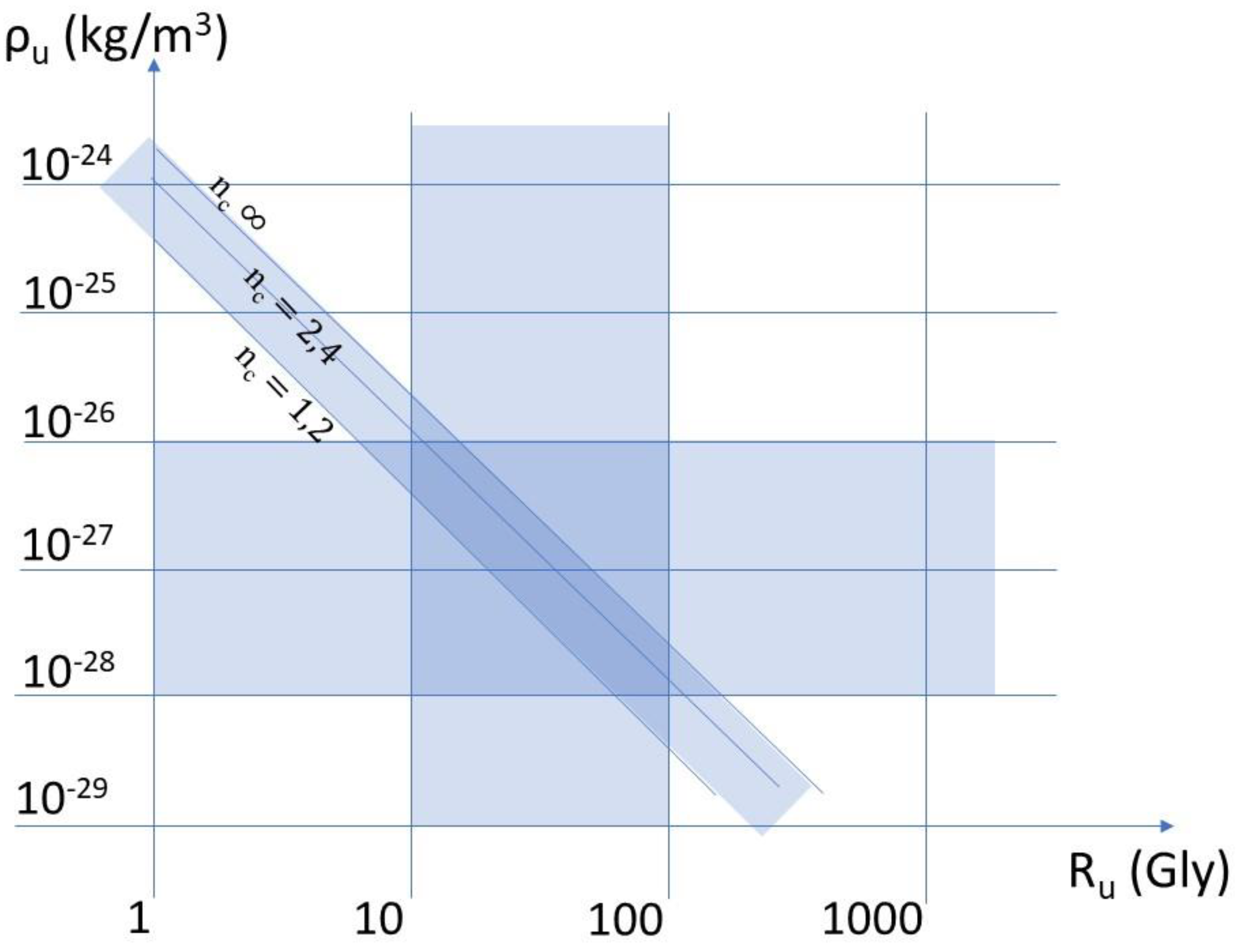
Figure 2.
Rotational velocities of spiral galaxies (Guy, 2024a). Two spiral galaxies were chosen from McGaugh (2014): the DDO 154 galaxy on the left and the NGC 1560 galaxy on the right. The rotational velocities of the stars are represented on the y-axis (km/s), their distance from the center of the galaxy is noted as R, on the x-axis (kpc). Two curves are shown for each galaxy: the dotted line represents the “measured” values (original points in the cited article); the solid line represents the values estimated on the basis of assumptions about the amount of baryonic matter and its distribution in the galaxy. As R increases, the velocities increase sharply, stabilize at a plateau, and then decrease slightly. The velocities in the ascending parts of the two curves have a constant ratio (the slopes are not strictly straight, but the ratio between the velocity values remains roughly constant). This ratio is the same on the plateaus, where it is particularly visible. In other words, we have AA’/AA” ≈ BB’/BB” ≈ CC’/CC” for each of the two galaxies. For DDO 154, the ratios are 2.3, 2.5, and 2.4, respectively; for NGC 1560, the ratios are 2.4, 2.3, and 2.3, respectively (approximate estimates). These are therefore also the same ratios as those observed in the two different galaxies.
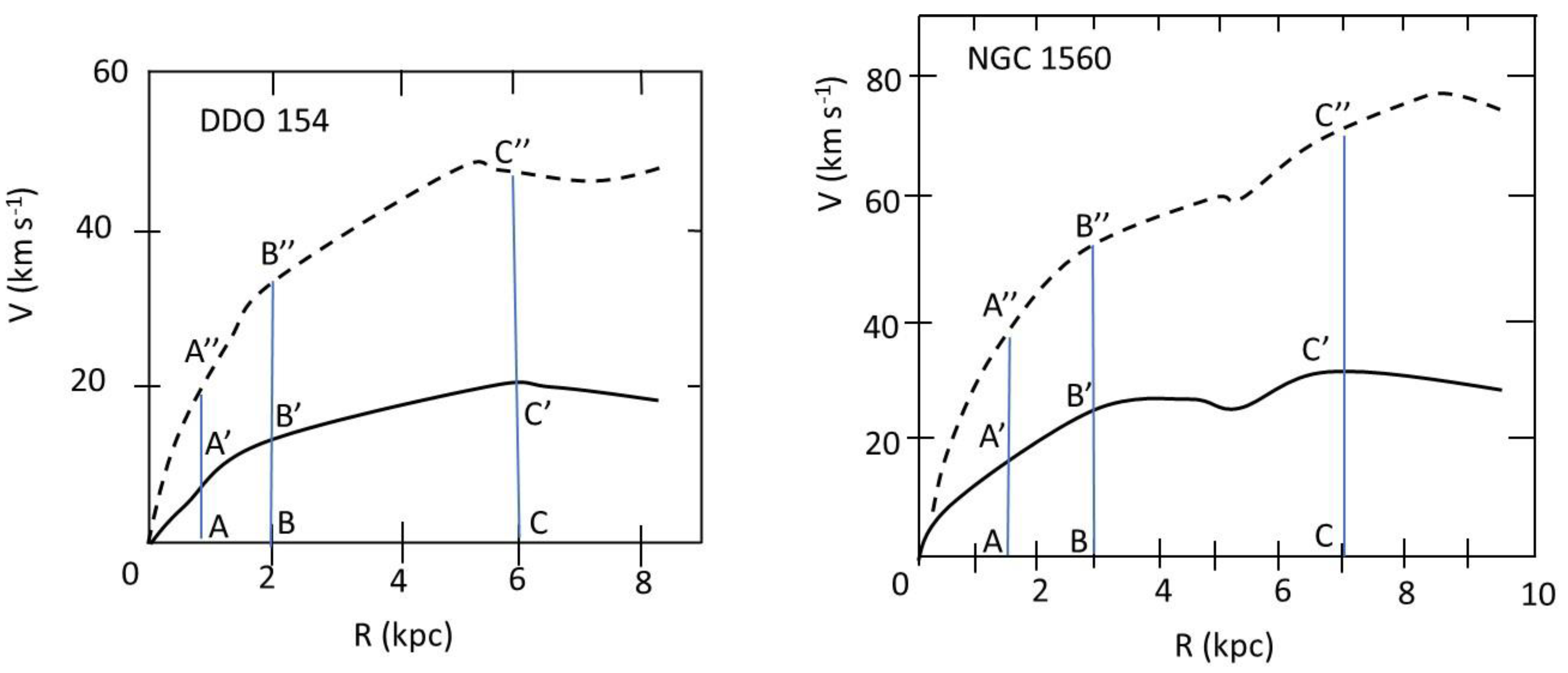
Figure 3.
Scale factor a(t) as a function of time for several universe models (Guy, 2024a). Horizontal axis: age from the present in billions of years. Vertical axis: scale factor a(t). The correspondence with redshift z is also indicated for z > 0. Redrawn from Aubert (2019). Three models are considered: the standard ΛCDM model (Ωm = 0.315, ΩΛ = 0.685), blue dotted curve; the standard Einstein De Sitter model (Ωm = 1, ΩΛ = 0), black dotted curve; our proposal (Einstein De Sitter model with a reduced Hubble constant, H0 /2.4), solid red curve. Like Aubert, we have taken H0 = 67 km/s/Mpc. The equation for the Einstein De Sitter model is a(t) = (3H0 t/2)2/3 + 1. It is interesting to note that the red curve and the blue curve are very close to each other for our local universe (0 < z < 1), whereas in the more distant past, a long duration, reaching some 10 Gyr (for a high z, reaching z = 20), appears. This may provide a comfortable latitude for galaxies to form and evolve in the early stages of a prolonged universe, while respecting the standard evolution of stars in later stages.
Disclaimer/Publisher’s Note: The statements, opinions and data contained in all publications are solely those of the individual author(s) and contributor(s) and not of MDPI and/or the editor(s). MDPI and/or the editor(s) disclaim responsibility for any injury to people or property resulting from any ideas, methods, instructions or products referred to in the content. |
© 2025 by the authors. Licensee MDPI, Basel, Switzerland. This article is an open access article distributed under the terms and conditions of the Creative Commons Attribution (CC BY) license (http://creativecommons.org/licenses/by/4.0/).
Copyright: This open access article is published under a Creative Commons CC BY 4.0 license, which permit the free download, distribution, and reuse, provided that the author and preprint are cited in any reuse.


