
Submitted:
15 September 2025
Posted:
16 September 2025
You are already at the latest version
Abstract
This study presents an integrated geospatial and hydrological assessment of flood patterns in Aweil East and South, located in Northern Bahr el Ghazal, South Sudan. Using HEC-RAS v6.6 Rain-on-Grid modeling, the research simulates rainfall-induced runoff across low-gradient catchments characterized by subsistence agriculture, grasslands, and seasonal wetlands. High-resolution datasets including the FABDEM v1.2 bare-earth elevation model and ESA World Cover land use classification were used to delineate watershed boundaries, estimate surface roughness, and calculate runoff volumes. Rainfall frequency analysis over a 110-year period was applied to determine return periods and hazard thresholds. A weighted Curve Number of 87.2 was derived from land cover proportions, enabling accurate runoff estimation using the SCS method. Results show that even frequent rainfall events with 1–2 year return periods can generate significant flood hazards due to minimal elevation change and poorly defined drainage channels. Flood hazard categories were evaluated using depth-velocity criteria from the Australian Rainfall and Runoff Guidelines, highlighting risks to settlements and infrastructure. The findings offer a robust framework for flood risk mapping, climate resilience planning, and disaster preparedness in vulnerable agro-pastoralist communities.
Keywords:
flood modeling
; rain-on-grid simulation
; hydrological analysis
; land use classification
; aweil catchment
Background Introduction
Aweil East and Aweil South are counties located in Northern Bahr el-Ghazal State, in the northwestern region of South Sudan. These areas lie within the western flood plains sorghum and cattle livelihoods zone, where the population is predominantly agro-pastoralist, relying on seasonal crop cultivation and livestock rearing for survival. Aweil East borders Sudan to the north and Abyei to the northeast, making it geopolitically significant and vulnerable to transboundary environmental and social pressures. Aweil South, situated to the southwest of Aweil East, shares similar ecological and socioeconomic characteristics, with flat terrain and poorly drained soils that make it highly susceptible to seasonal flooding.(Gakai, Waweru et al. 2025)
The region experiences a tropical savanna climate, with distinct wet and dry seasons. Rainfall variability, coupled with low-gradient topography, contributes to frequent sheet flooding, which disrupts agriculture, displaces communities, and damages infrastructure. The population is largely composed of Rek Dinka (Malual: Abiem) ethnic groups, and both counties have witnessed significant displacement due to conflict and climate shocks. Despite these challenges, local markets such as Malualkon, Akuem, and Warawar serve as vital economic hubs, connecting rural producers to broader trade networks.
Understanding the hydrological and geospatial dynamics of Aweil East and South is essential for developing sustainable flood management strategies, improving agricultural resilience, and guiding humanitarian interventions in this climate-sensitive region.(Ba, Usman et al. 2025, Wanjiru, Kathuri et al. 2025)
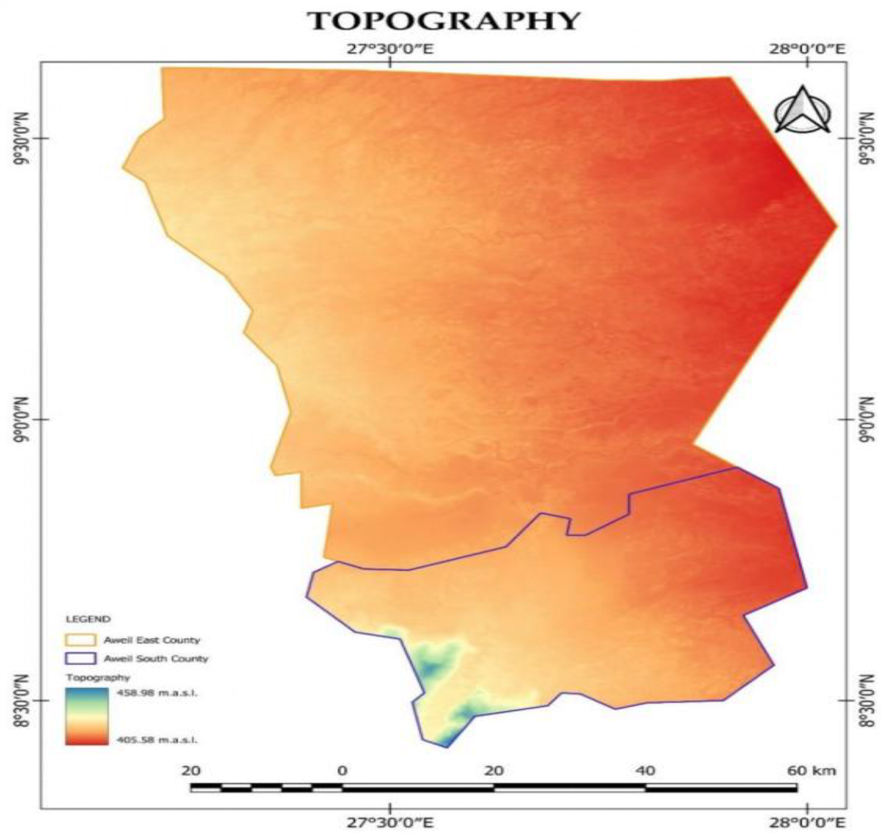
The area encompassing Aweil East and Aweil South counties lies within the Sudanian savanna ecoregion, a landscape defined by gently undulating plains that sit between 400 and 500 meters above sea level (Survey of South Sudan, 2021). Despite its seemingly uniform appearance, this terrain plays a pivotal role in shaping the region’s hydrological behavior. Seasonal wetlands, locally known as toiches, act as natural water retention basins, rapidly filling during the rainy season and causing prolonged inundation that can persist for months (FAO, 2023). These physiographic features, influenced by the area’s location within the White Nile sub-basin, offer both agricultural promise and heightened flood vulnerability, making water management a critical concern.(Gakai, Waweru et al. 2025) (Meng, Dong et al. 2024)
Further analysis reveals that the region’s slope angles rarely exceed 1% (JAXA, 2023), resulting in a landscape with extremely low gradient. This subtle topography has significant consequences for water flow, particularly in Aweil South, where communities are concentrated along the floodplains of the Lol River. Here, floodwaters tend to stagnate for three to five months annually (IOM, 2023), exacerbated by the lack of defined drainage channels. The result is widespread sheet flooding that disrupts farming and damages homes. These conditions highlight the urgent need for engineered drainage systems tailored to the region’s unique physiographic profile, to reduce the long-term impacts of seasonal flooding.(Gakai, Waweru et al. 2025, Kipkemoi, Sitati et al. 2025)
Methodology
The methodology employed in this study integrates geospatial analysis with hydrological modeling to assess flood risk across Aweil East and South. Rainfall data spanning over a century was compiled from historical records and satellite-based sources such as CHIRPS and GPR stations. Using GIS tools, watershed boundaries were delineated from Digital Elevation Models (DEMs), and land cover classifications were extracted from Sentinel-2 imagery. These spatial datasets were layered to identify terrain characteristics, drainage networks, and land use patterns that influence runoff behavior. The Soil Conservation Service (SCS) Curve Number method was applied to estimate surface runoff based on land cover, soil type, and rainfall intensity, providing a quantitative foundation for flood modeling.(Gakai, Waweru et al. 2025)
To evaluate the frequency of extreme rainfall events, the study employed the Weibull plotting position formula ( Tr = \frac{n + 1}{R} ), where Tr is the return period, n is the number of years in the dataset, and R is the rank of the rainfall event. This statistical approach enabled the construction of a rainfall frequency curve, illustrating the likelihood of high-magnitude events over time. Hydrographs were generated to simulate peak discharge at the catchment outlet, offering insight into flood timing and volume. The combined use of spatial mapping, historical rainfall analysis, and hydrological simulation provides a robust framework for identifying flood-prone zones and informing climate-resilient planning in Aweil’s low-gradient landscape.(Lai, Xie et al. 2003)

Table 1.
Global datasets used in the flood modelling.
| Dataset | Purpose | Horizontal Resolution | Original Source | Comments |
| FABDEM | Define Topography | 30 m | TandemX | Bare earth: Vegetation and buildings removed |
| WorldCover | Land use, friction and Infiltration Curve Number | 10 m | Sentinel 1 & 2 | 2021 date |
| HYSOG | Soil type: Infiltration Curve Number | 250 m | FAO +++ | - |
| River Centrelines | River channels | +- 2m | Hand digitised river centrelines using Bing and Google satellite photos | Used to burn in channels that are not explicit in the DEM (bed elevation and width and depth of channel). Also provides river roughness values in model |
| GPM | Spatially and temporally varied precipitation input driver (source of water in model) | 10km / 0.1 Degree | Global Precipitation Mission (IMERG) |
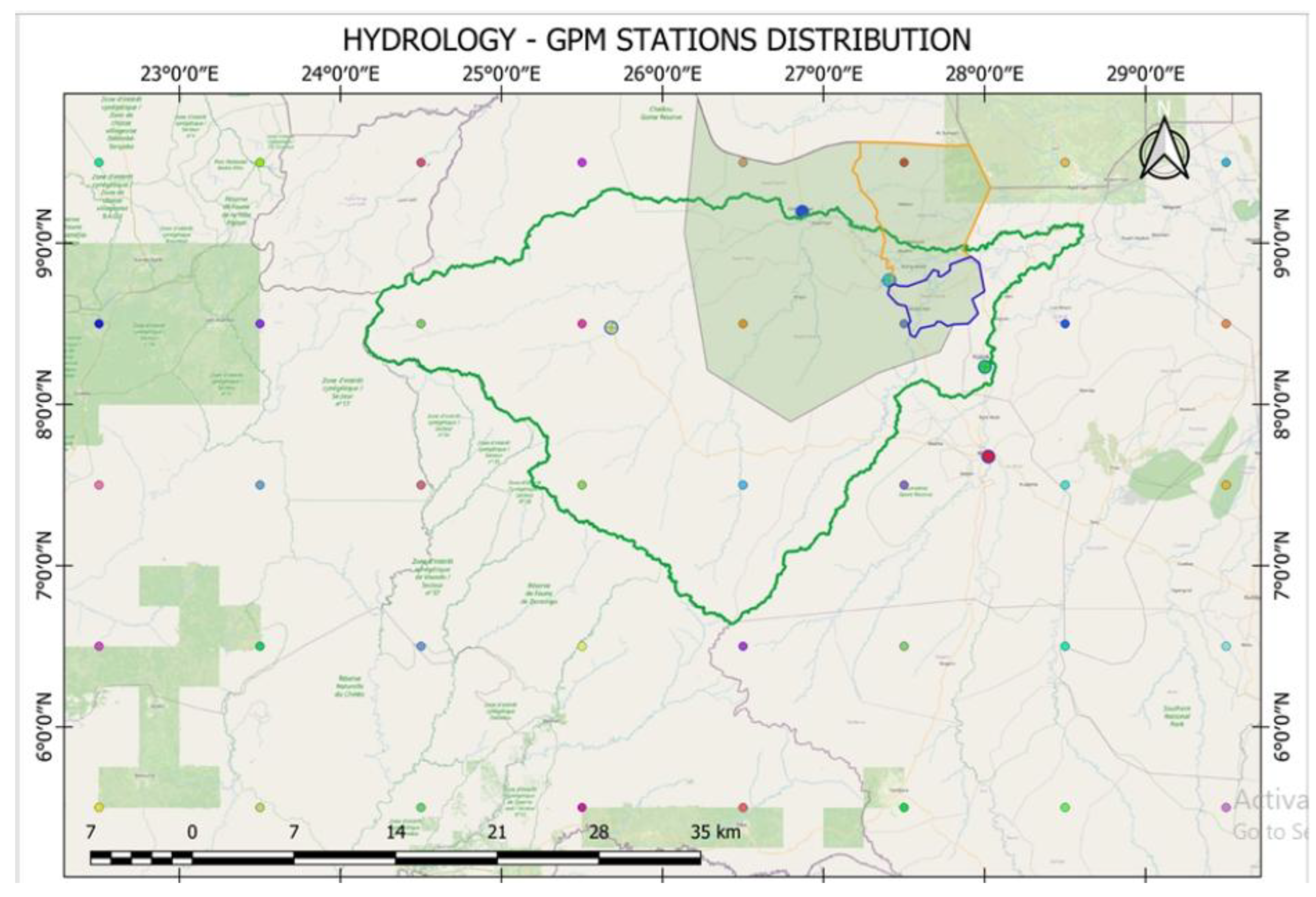
GPM rainfall data (Appendix II), was downloaded at 17 locations(see Figure 6), within or adjacent to the catchments.
Physiography, Topography and Drainage Patterns
Figure 1.
Aweil East and Aweil South Topography.
Geological Composition
Figure 2.
Aweil East and Aweil South Geology.
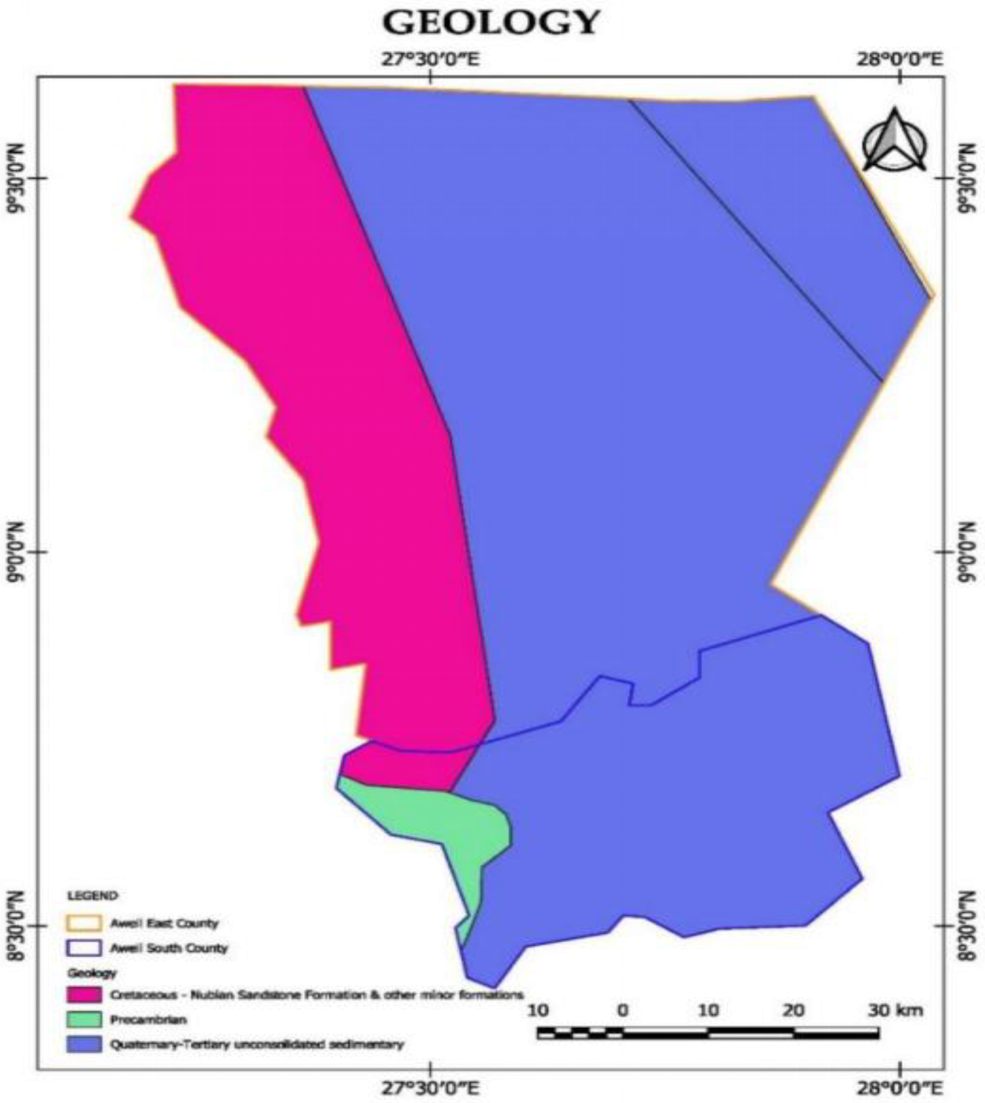
Beneath the surface of the project area lies a geologically intricate foundation shaped by layers of Quaternary alluvial deposits—primarily clays, silts, and sands—that blanket older Cretaceous-era sedimentary formations forming the region’s basement (USGS, 2022). These clay-rich upper layers exhibit low permeability, which severely limits water infiltration during intense rainfall, leading to rapid surface runoff. In certain pockets, the presence of lateritic soils further complicates infrastructure development due to their variable strength and moisture sensitivity (Batjes 2022). Together, these geological features play a direct role in amplifying flood risks across the landscape.
Soil Characteristics and Erosion Risks
Figure 3.
Aweil East and Aweil South Soils.
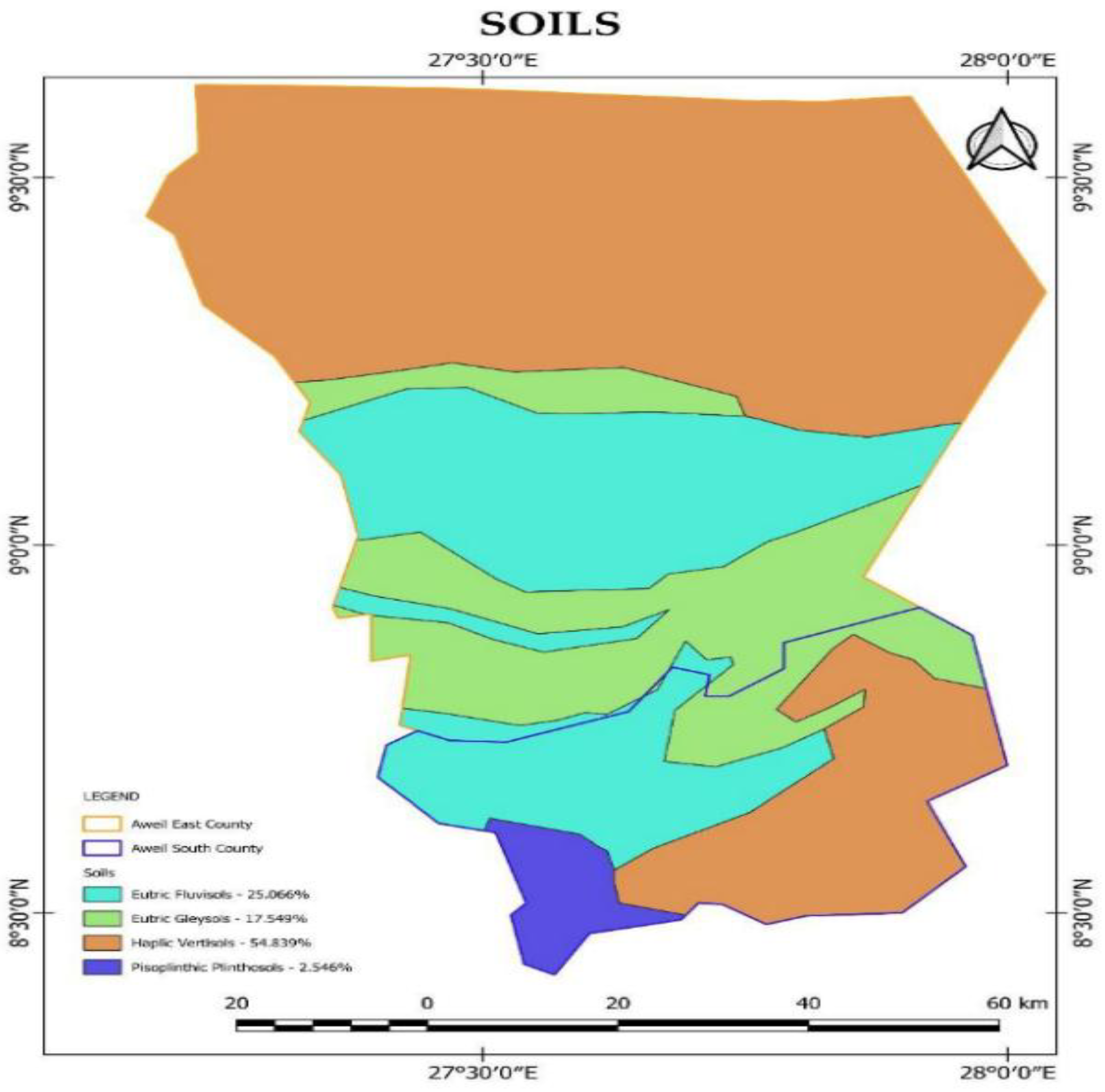
The dominant soil types in the region—vertisols and fluvisols—pose a complex mix of benefits and challenges for local communities (Batjes, Calisto et al. 2024). Vertisols, rich in clay and known for their dramatic shrink-swell behavior, become nearly impermeable during the rainy season, hindering water infiltration, while developing deep fissures in dry conditions. Fluvisols, formed by seasonal flood deposits, offer fertile ground for cultivation but are highly prone to erosion. Alarmingly, recent studies show a 12% decline in topsoil since 2015, largely driven by deforestation and unsustainable farming practices (Gibbs, Rose et al. 2025)This degradation not only undermines crop yields but also intensifies flood risks by increasing sedimentation in local waterways.
Land Use and Land Cover Dynamics
Figure 4.
Land Use and Land Cover for Aweil East and Aweil South Counties.
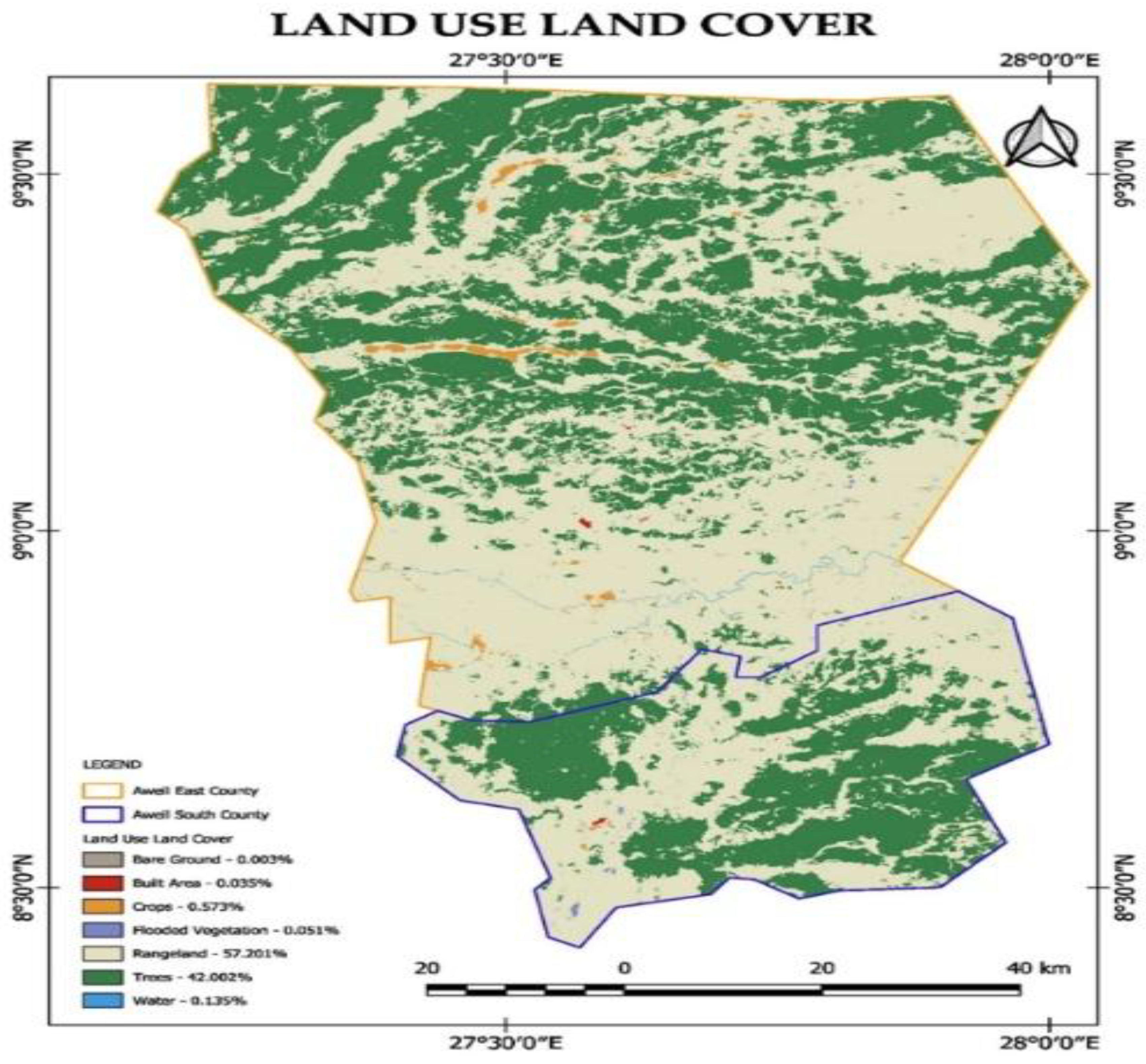
The landscape of Aweil East and Aweil South illustrates a fragile equilibrium between human livelihoods and ecological integrity, with roughly 60% of the land devoted to subsistence farming—mainly sorghum and maize—while grasslands and savanna, vital for grazing, make up 20% of the cover (Sentinel-2 analysis, 2023). Settlements and wetlands occupy another 15%, and the remaining 5% comprises degraded forest areas, reflecting a steep decline from historical forest coverage. Alarmingly, deforestation continues at an estimated rate of 3% annually, driven by charcoal production and expanding agriculture (GFW, 2023), which severely undermines the region’s natural flood-buffering capacity by diminishing tree cover that would otherwise absorb and gradually release excess water
Rainfall Variability
Table 1.
Weather Stations.
| # | gid | STATION | DATE ESTABLISHED | LAST UPDATED |
| 1 | 11 | RAGA | 1941-01-01 | 2021-01-09 |
| 2 | 3 | Gokmachar (Awiel) | 2024-12-10 | 2025-01-16 |
| 3 | 1 | Aweil Rice Scheme | 2024-12-09 | 2025-01-16 |
| 4 | 6 | Kuajok town- (Angui) near FAO Office (SMoAF) | 2024-12-07 | 2025-01-16 |
| 5 | 15 | WAU | 1941-01-01 | 2023-06-07 |
Precipitation patterns in Aweil East and Aweil South exhibit a mix of seasonal regularity and alarming variability, with annual rainfall averaging between 800–1,200 mm but fluctuating by as much as ±30% from year to year (CHIRPS, 2024). In recent seasons, the region has experienced increasingly extreme rainfall events, such as a staggering 150 mm recorded in a single day in 2023—nearly twice the historical daily maximum of 80 mm (World Bank Climate Portal, 2023). These concentrated downpours exceed the land’s natural absorption capacity, triggering flash floods that disrupt livelihoods and strain local infrastructure.Hydrology and Flood Risks(Du, Tan et al. 2024)
The Lol River system functions as the central drainage artery for Aweil East and Aweil South, with peak discharges reaching up to 450 cubic meters per second during intense rainfall events Hydrological models reveal that nearly 40% of these floodwaters originate from upstream catchments in Sudan, underscoring the transboundary nature of the flood threat and the need for cross-border collaboration. The consequences are profound—recent assessments indicate that as much as 75% of cropland in Aweil South becomes submerged during major floods, severely disrupting food production and livelihoods .This intricate flood regime, shaped by both local precipitation and external inflows, demands integrated and cooperative water management strategies to mitigate its recurring impacts. (Gakai, Waweru et al. 2025)
The outlet of the main catchment covering mostly Aweil South County, was determined to be a point on the River Lol just outside Northern Bahr-El-Ghazal (just outside the corner of the state boundary at Malek).
Figure 5.
Catchment map and drainage for project area.
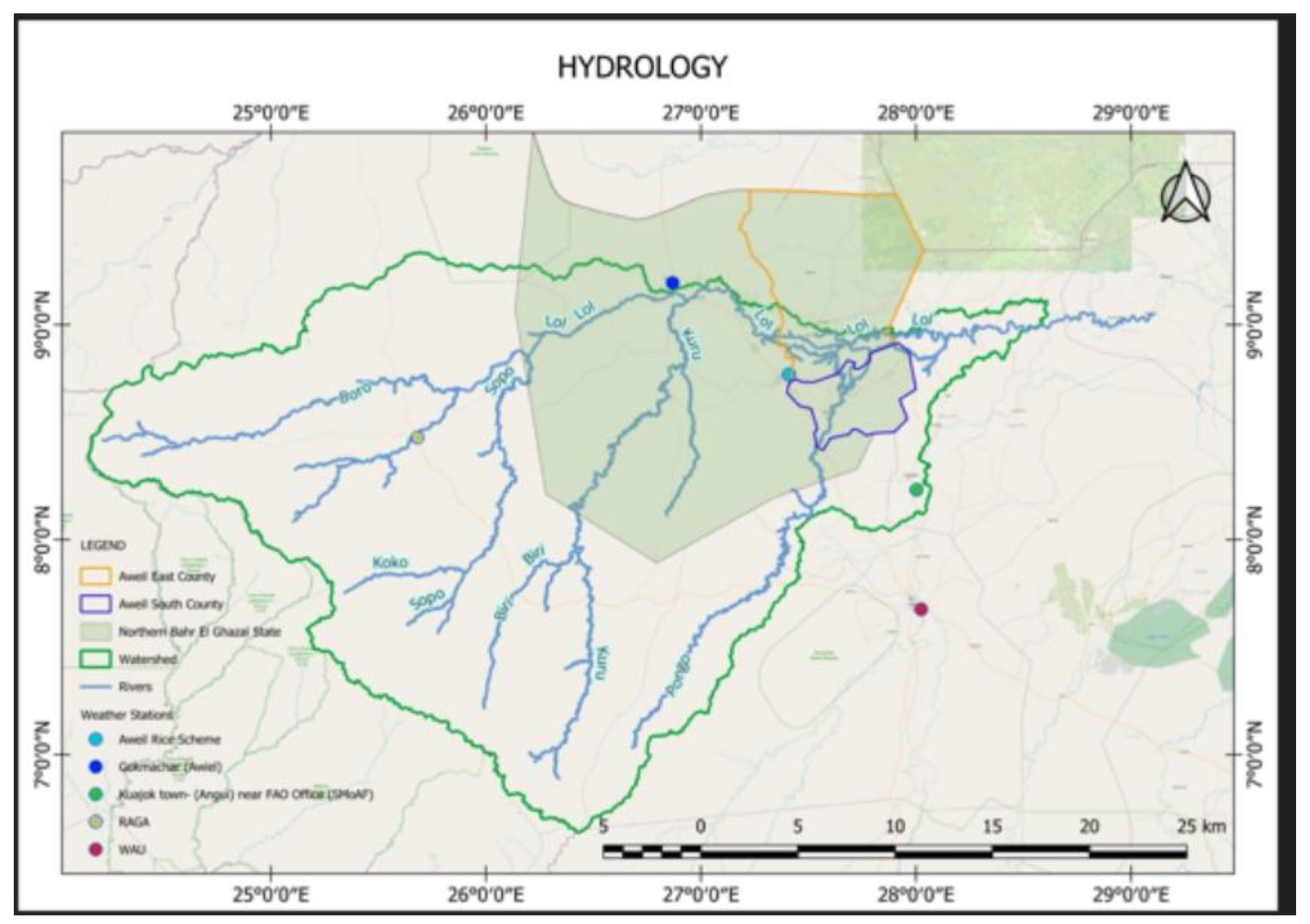
The catchment was determined by delineation using QGIS as in the map of Figure 5.
The map shows part of the catchment area within which the sub-projects are found, mostly in Aweil South, the drainage systems with the rivers and their tributaries, and the locations of five weather stations relevant to the project.
Figure 6.
Location of GPM satellite rainfall stations.
Hydrological Analysis
Adjustment of GPM Satellite Rainfall Data
Satellite rainfall data is not always representative of the actual rainfall depths and intensities of observed ground data. Also, observed rainfall data corresponding to the flooding of 2024 were not available. Monthly rainfall totals were however available for Wau(1961-2015) and Malakal(1961-2013). (Onyutha, Tabari et al. 2016)With reference to Table 1 and Table 2, these were then averaged for each month. Monthly totals were also computed for GPM1 to GPM17. The averages for each month for GPMs and ground rainfall were then computed. These were then correlated to GPM data (Figure 7). The correlation of GPM to ground data was found to y = 1.1177x - 0.531 where y is the GPM rainfall and x the average of GPM and ground data. This was considered a reasonable conversion for GPM to ground data. Hence GPM data was adjusted to ground conditions by multiplying with 1.117. These results were used in the model.
However, peak discharges derived from rainfall using the SCS curve number method were analysed for frequency and return periods at Table 4
Table 2.
Monthly totals of Malakal, Wau, GPM rainfalls compared.
| MONTH | JAN | FEB | MAR | APR | MAY | JUN | JUL | AUG | SEP | OCT | NOV | DEC |
| Malakal | 0.00000 | 0.23962 | 7.29811 | 28.14528 | 84.26226 | 116.96604 | 153.37170 | 165.05769 | 125.40377 | 81.78302 | 5.21538 | 0.00000 |
| Wau | 0.84815 | 2.55556 | 15.30185 | 63.00556 | 122.10962 | 167.94528 | 187.30192 | 208.86346 | 178.37059 | 115.99608 | 17.50392 | 0.79020 |
| AV WAU/MALAKAL | 0.42407 | 1.39759 | 11.29998 | 45.57542 | 103.18594 | 142.45566 | 170.33681 | 186.96058 | 151.88718 | 98.88955 | 11.35965 | 0.39510 |
| GPM | 0.13790 | 0.69785 | 19.25508 | 79.51752 | 88.88677 | 161.57172 | 221.66864 | 233.45133 | 203.32345 | 141.00559 | 7.48661 | |
| AV GRD/GPM | 0.28098 | 1.04772 | 15.27753 | 62.54647 | 96.03636 | 152.01369 | 196.00273 | 210.20596 | 177.60531 | 119.94757 | 9.42313 | 0.39510 |
| GPM | 0.13790 | 0.69785 | 19.25508 | 79.51752 | 88.88677 | 161.57172 | 221.66864 | 233.45133 | 203.32345 | 141.00559 | 7.48661 |
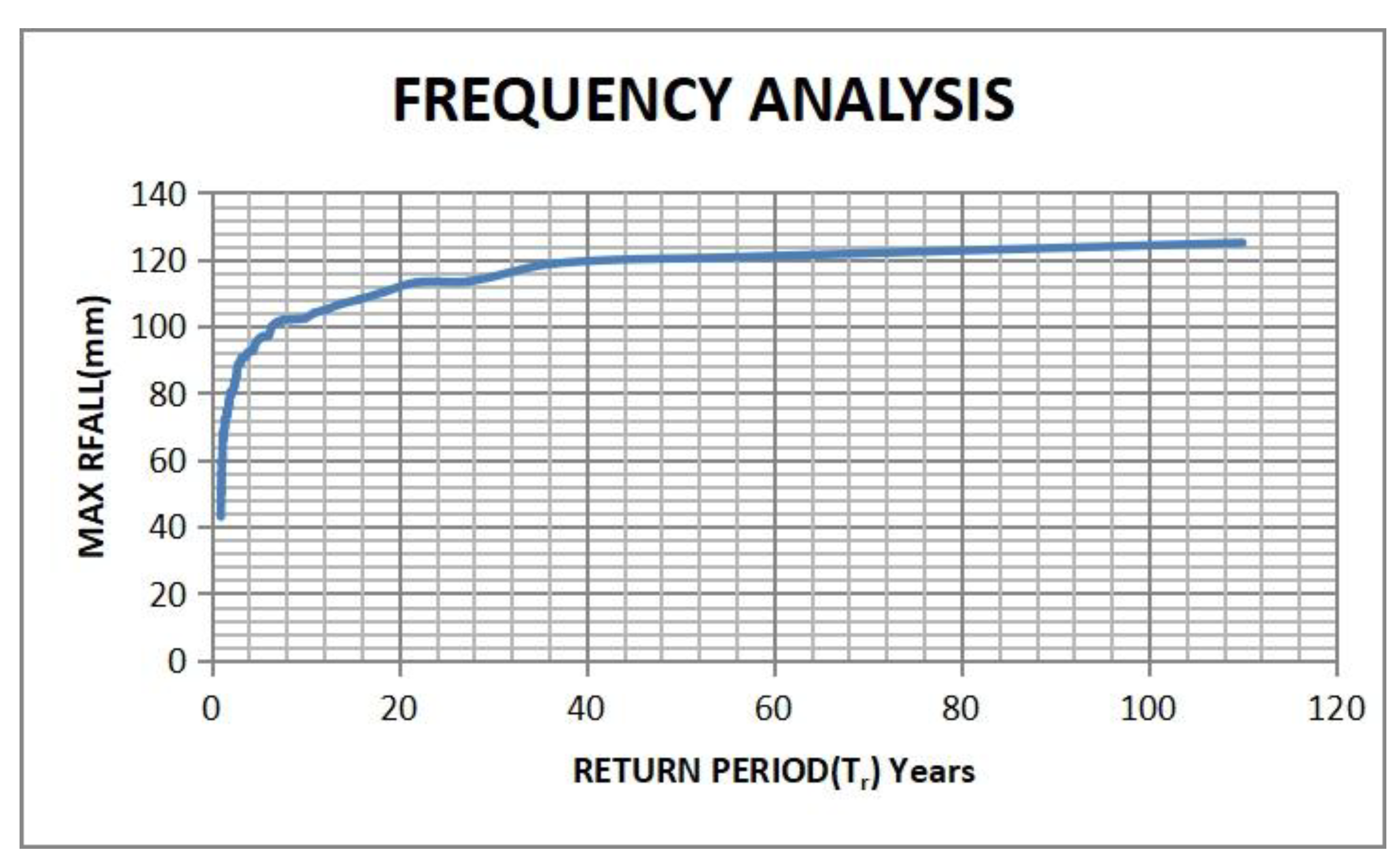
Figure 7.
Frequency analysis for Raga and Wau rainfall using Weibull formula.
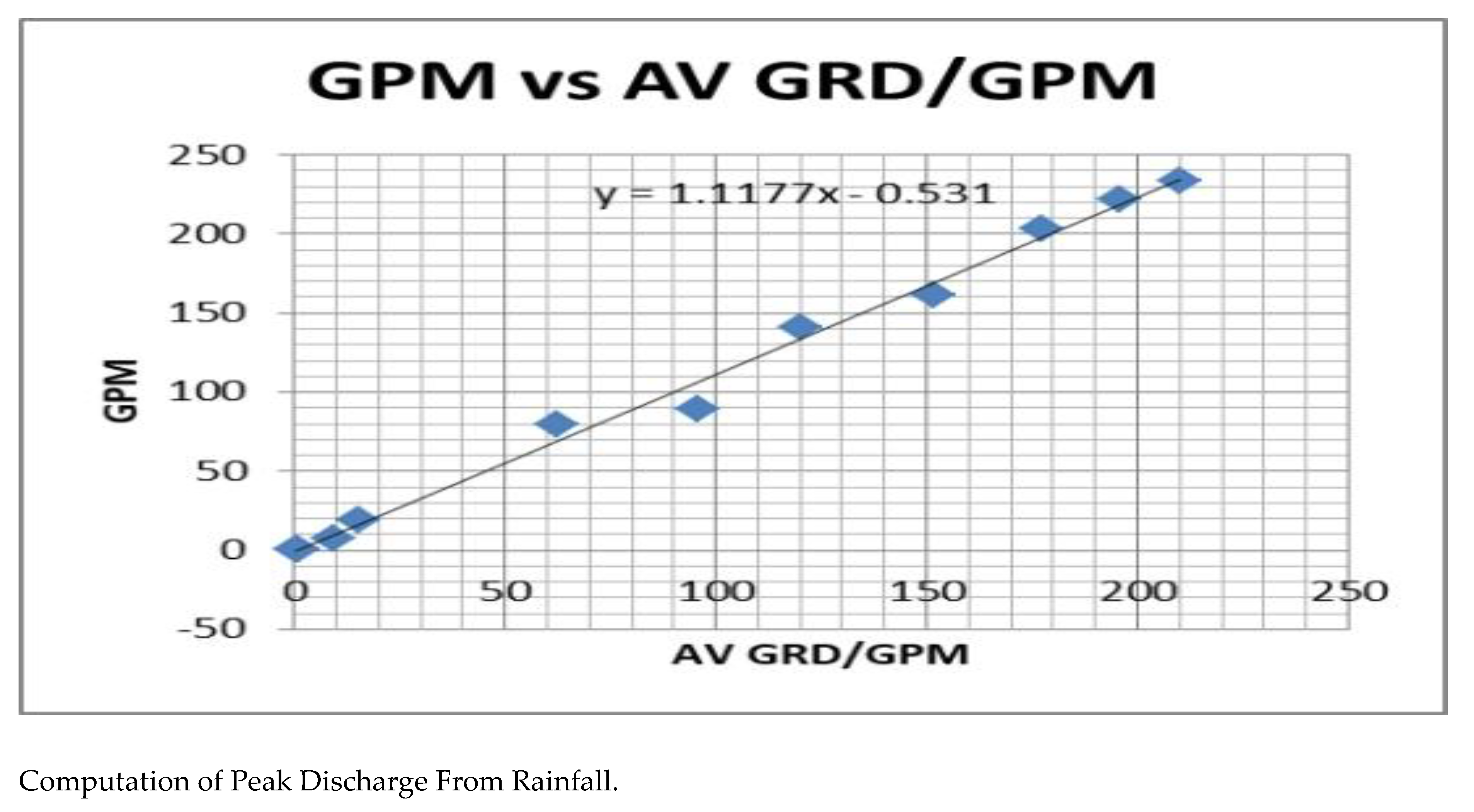
Figure 8.
Rainfall Frequency Analysis from Wau and Raga averages.
Computation of Peak Discharge From Rainfall.
Using Scs Curve Number Method
From the analysis above the 100 year return rainfall is 120.65 mm.
Catchment area computed using QGIS = 73,303.64 km²
The curve number (CN) for Aweil South can be computed from the landuse/landcover and soil properties as follows:
The Curve Number is a dimensionless value from 0–100 that estimates how much rainfall becomes runoff. It’s used in the SCS (Soil Conservation Service) method and depends on:
- Land Use / Land Cover (LULC)
- Soil Type / Hydrologic Soil Group (HSG)
- Hydrologic Condition (good/fair/poor)
- Antecedent Moisture Condition (AMC I–III)
Soils
According to global soil maps:
Aweil South is largely clayey soils with slow infiltration, generally classified as Hydrologic Soil Group D (HSG-D), the worst-case for runoff.
Land Use
Based on satellite imagery and known land use patterns in Northern Bahr el Ghazal, the landscape is characterized primarily by subsistence agriculture, fallow fields, and grasslands. Additionally, there are pockets of bushland/woodland and wetlands located in natural depressions.
To estimate runoff potential, standard NRCS Curve Number (CN) values for Hydrologic Soil Group D (HSG-D) were applied. The CN values for various land cover types are summarized below:
Table 3.
GRD vs GPM R Fall.
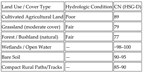
To derive a weighted Curve Number, the following land cover proportions were assumed:
- 50% cultivated farmland → CN = 89
- 30% grassland/bushland → CN = 79
- 10% wetlands/depressions → CN = 98
- 10% bare/fallow land → CN = 92
The weighted CN is calculated as: CN = (0.5 × 89) + (0.3 × 79) + (0.1 × 98) + (0.1 × 92) = 44.5 + 23.7 + 9.8 + 9.2 = 87.2
This value reflects the composite runoff potential of the catchment and is used in hydrological modeling to estimate surface runoff during rainfall events.
To estimate how much rainwater turns into runoff, we use the SCS runoff equation. With a rainfall depth of 120.65 mm and a Curve Number (CN) of 87.2, the runoff depth (Q) comes out to 85.2 mm, or 0.0852 meters. Multiplying this by the catchment area of 73,303.64 km² gives a total runoff volume of about 6.25 billion cubic meters. To convert this volume into flow rate (discharge), we estimate how long the runoff lasts. Assuming it drains over 48 hours (172,800 seconds), the average discharge is around 36,156 m³/s. Applying a peaking factor of 2 (to account for storm intensity), the peak discharge is approximately 72,312 m³/s.
In contrast, the flood model for Aweil South indicates a peak discharge of 2,093.748 m³/s. By estimating the average discharge as half of the peak value (1,046.874 m³/s), the total runoff volume over a 48-hour period is approximately 181 million cubic meters. When this volume is divided by the catchment area, it yields a runoff depth of 2.47 mm. Applying the SCS method with a Curve Number (CN) of 87.2, the corresponding rainfall depth required to generate this runoff is estimated to be around 18.5 mm.
Based on the rainfall frequency plot for the two sites, the peak rainfall used in the flood model corresponds to a return period of approximately 1 to 2 years. This suggests that such events are relatively frequent, occurring every one to two years, yet they still pose a significant hazard. When compared to the modeled flood of 72,312 m³/s resulting from a 100-year rainfall event of 120.65 mm, it becomes clear that careful interpretation of the data is essential. A short-duration 100-year rainfall does not necessarily produce a 100-year flood; conversely, a 10-year rainfall sustained over a longer duration could potentially result in a flood of similar magnitude.
Figure 9.
Rainfall for each month for GPM1 to GPM17.
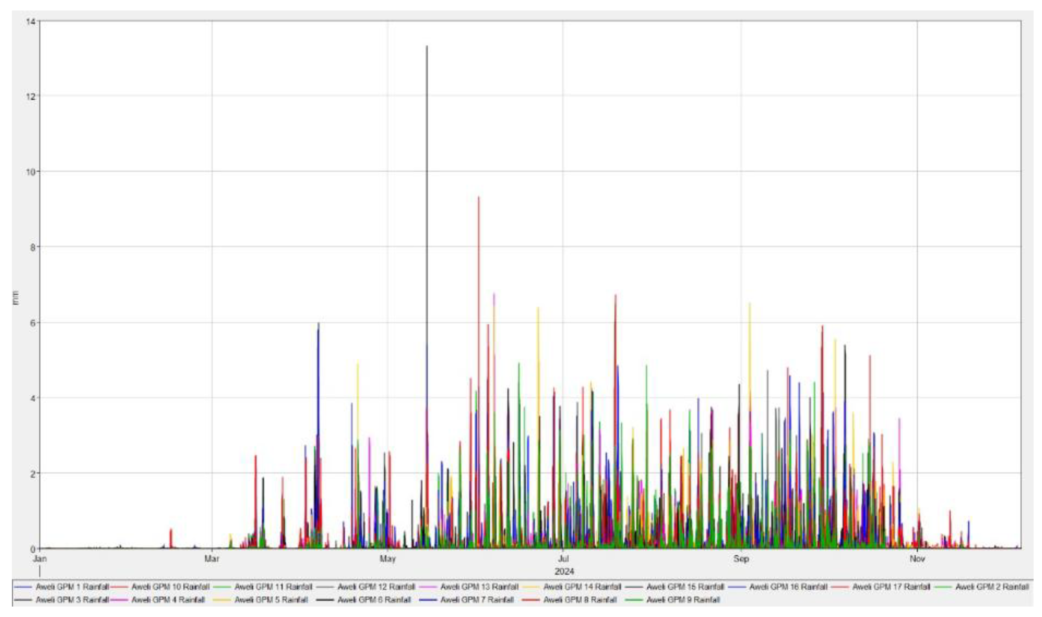
Figure 10.
Sums of rainfall for each GPM to determine rainiest month.
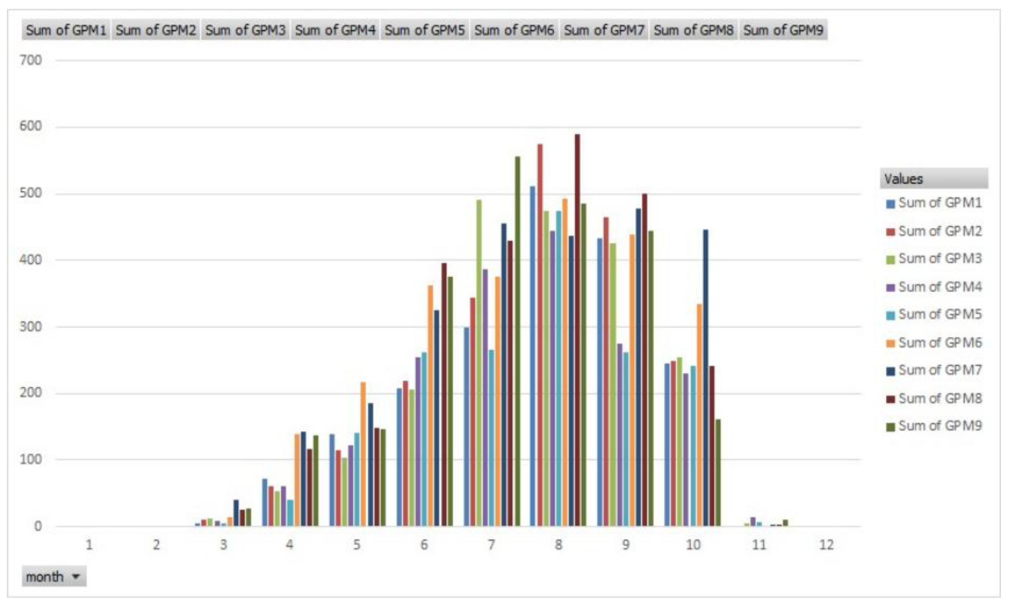
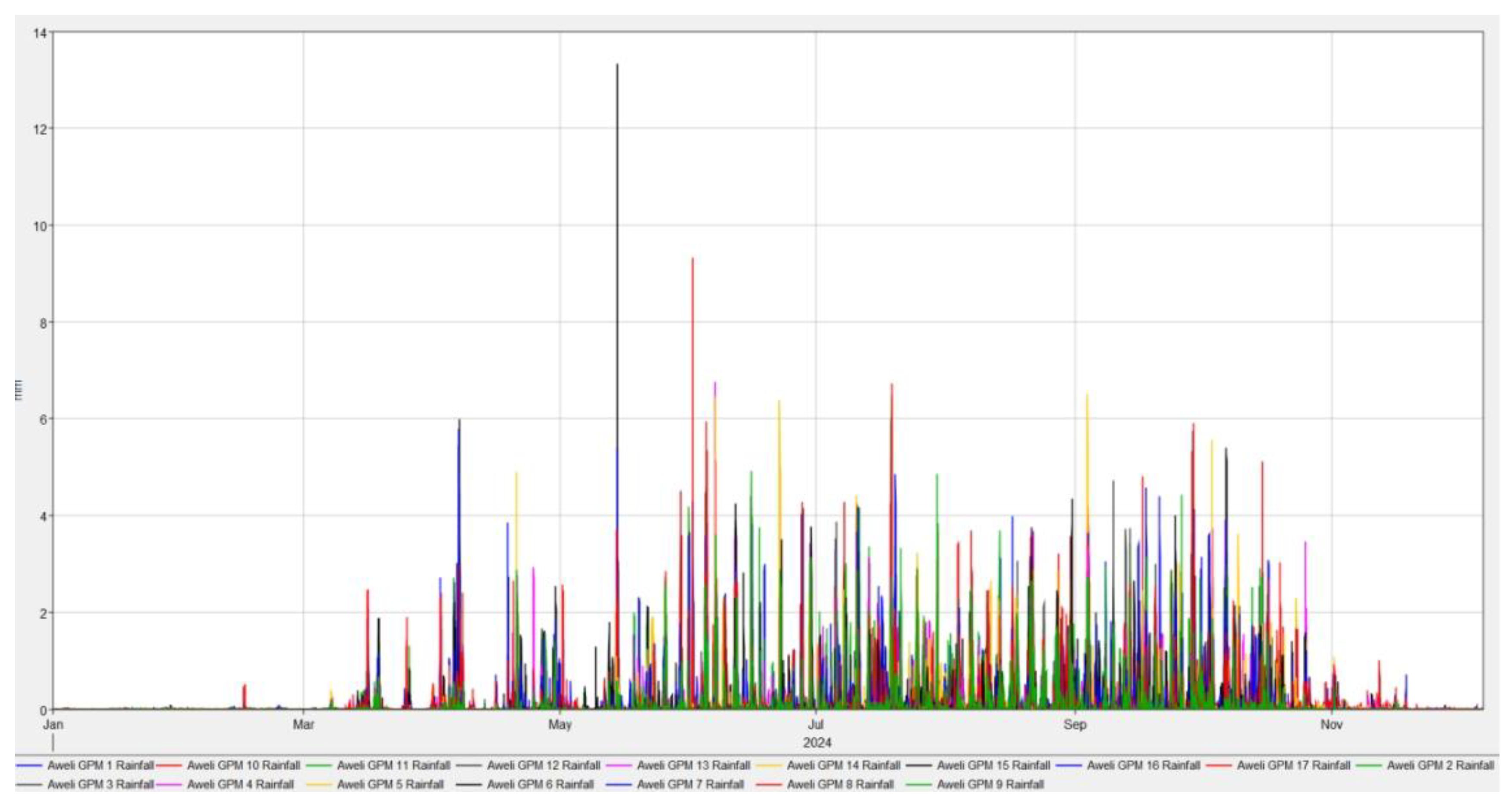
Figure 11.
Pluviographs for GPM1 to GPM17 for 2024.
The bar graph presents monthly rainfall data from January to November 2021, measured in inches and categorized by eight different sources labeled “Award GPR 1” through “Award GPR 8,” each represented by a distinct color. The x-axis displays the months, while the y-axis ranges from 0 to 14 inches, allowing for clear visualization of rainfall trends across time and sources. A pronounced spike in rainfall is observed in May, with several sources recording nearly 12 inches—almost double the historical monthly maximum—indicating a significant weather anomaly. The remaining months show more moderate and variable rainfall levels, with notably lower totals in February and September. This visual comparison is valuable for identifying seasonal patterns and anomalies, which are critical for flood modeling and hydrological planning in regions like Aweil. From the analysis, the month of August was found to have received the most total rainfall in the month and therefore the highest magnitude of flooding. Hence the flood modeling focused on the month of August 2024
Flood Modeling
HEC-RAS v6.6 Rain-on-Grid flood modeling was employed to simulate runoff and flood dynamics hydrodynamically within the two study catchments. This modeling approach utilizes the entire catchment area and incorporates both infiltration and surface runoff processes, along with the hydraulic behavior of river channels. It applies spatially variable precipitation directly across the catchment, eliminating the need for predefined river flow hydrographs.
Accurate representation of land topography is essential for reliable flood modeling. In this study, a bare-earth Digital Elevation Model (DEM) was used to capture terrain features without interference from vegetation or built structures. Specifically, the FABDEM v1.2 dataset (Hawker, Uhe et al. 2022)was selected, as it excludes trees and buildings, making it particularly well-suited for hydrodynamic flood simulations.
Figure 12.
FABDEM topography for Aweil South catchment, with main river channels.
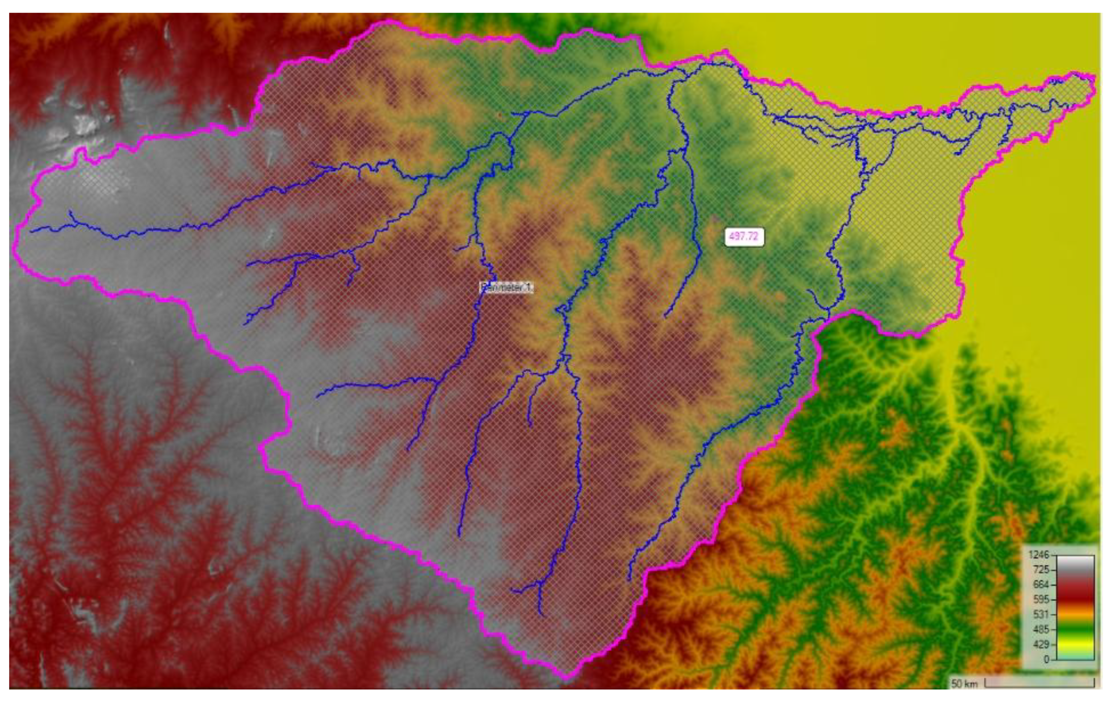
Figure 12 illustrates the flood model computation mesh, which employs a default grid resolution of 200 meters. Higher-resolution calculation cells, measuring 25 meters, are applied along the river centerlines to enhance the accuracy of flow simulations in critical drainage pathways.
The accompanying topographic map presents elevation data and delineates the watershed using a color gradient ranging from red (representing higher elevations) to green and yellow (indicating lower elevations), with elevation values spanning from 435 to 1266 meters. A magenta boundary outlines the watershed, while blue lines trace the river and stream networks within it. Two labeled elevation points—403.72 and 403.8474 meters—mark specific low-lying zones in the basin. The terrain is gently sloped, characteristic of low-gradient landscapes that influence water movement and flood behavior. Such configurations are typically vulnerable to sheet flooding, where water disperses widely due to minimal elevation change and poorly defined drainage channels.
Map Layers Generated
Land Cover
Figure 13.
Land cover/landuse layer.
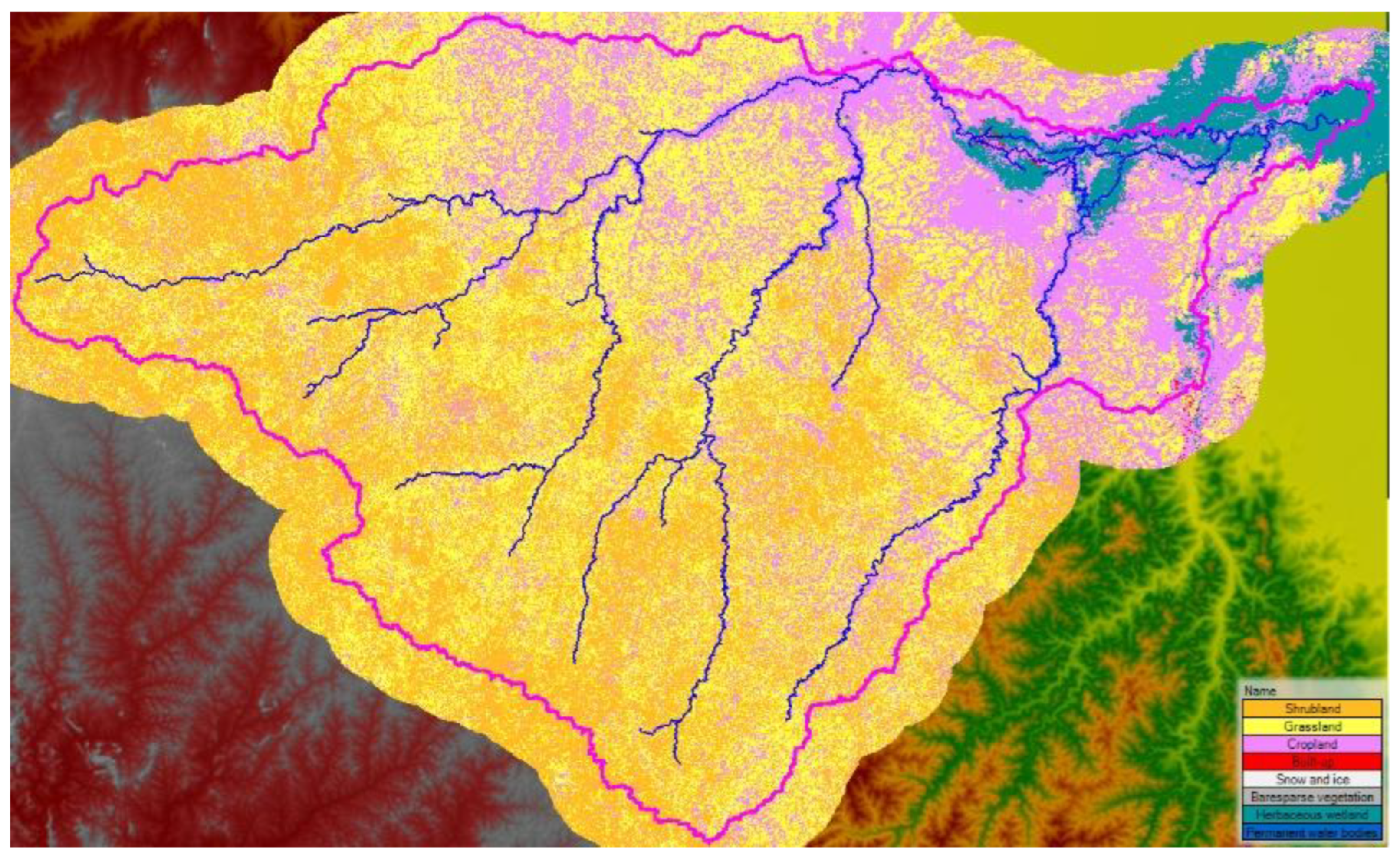
To assign Manning’s roughness coefficients for hydrological modeling, a land cover layer was incorporated as shown in Figure 6.4. The dataset used was the ESA WorldCover 10m 2021, which provides high-resolution global land cover classification. The corresponding land cover categories and their associated roughness values are presented in Table X.
The map offers a detailed representation of land cover and topography within a clearly defined watershed, outlined in bold magenta. Distinct land cover types are visualized using specific colors: cropland in yellow, grassland in green, shrubland in blue, evergreen needleleaf forest in orange, and barren or non-vegetated areas in gray. A network of rivers and streams, highlighted in dark blue, traverses the basin and intersects various land cover zones. The underlying topography is depicted using shaded relief, with red hues indicating higher elevations and green hues representing lower terrain. This spatial configuration is critical for understanding surface roughness, flow resistance, and the interaction between land cover and hydrological processes.
Soils
Figure 14.
Soil Layer.
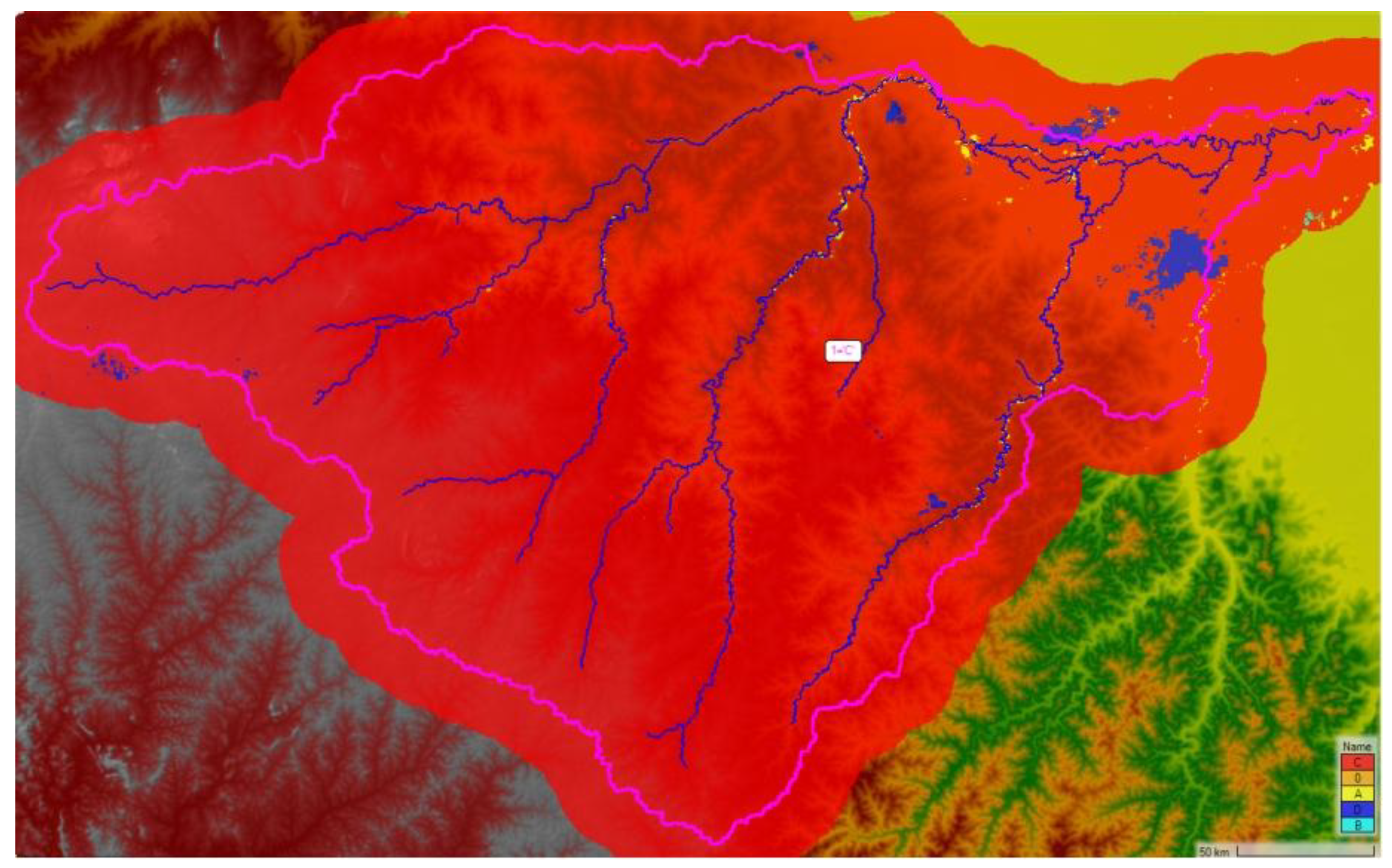
The SCS curve number method was used in computation of soil losses to infiltration in runoff generation. The soil layer used was the RFA1 Hydrologic SoilGroup 2020. See Figure 14.
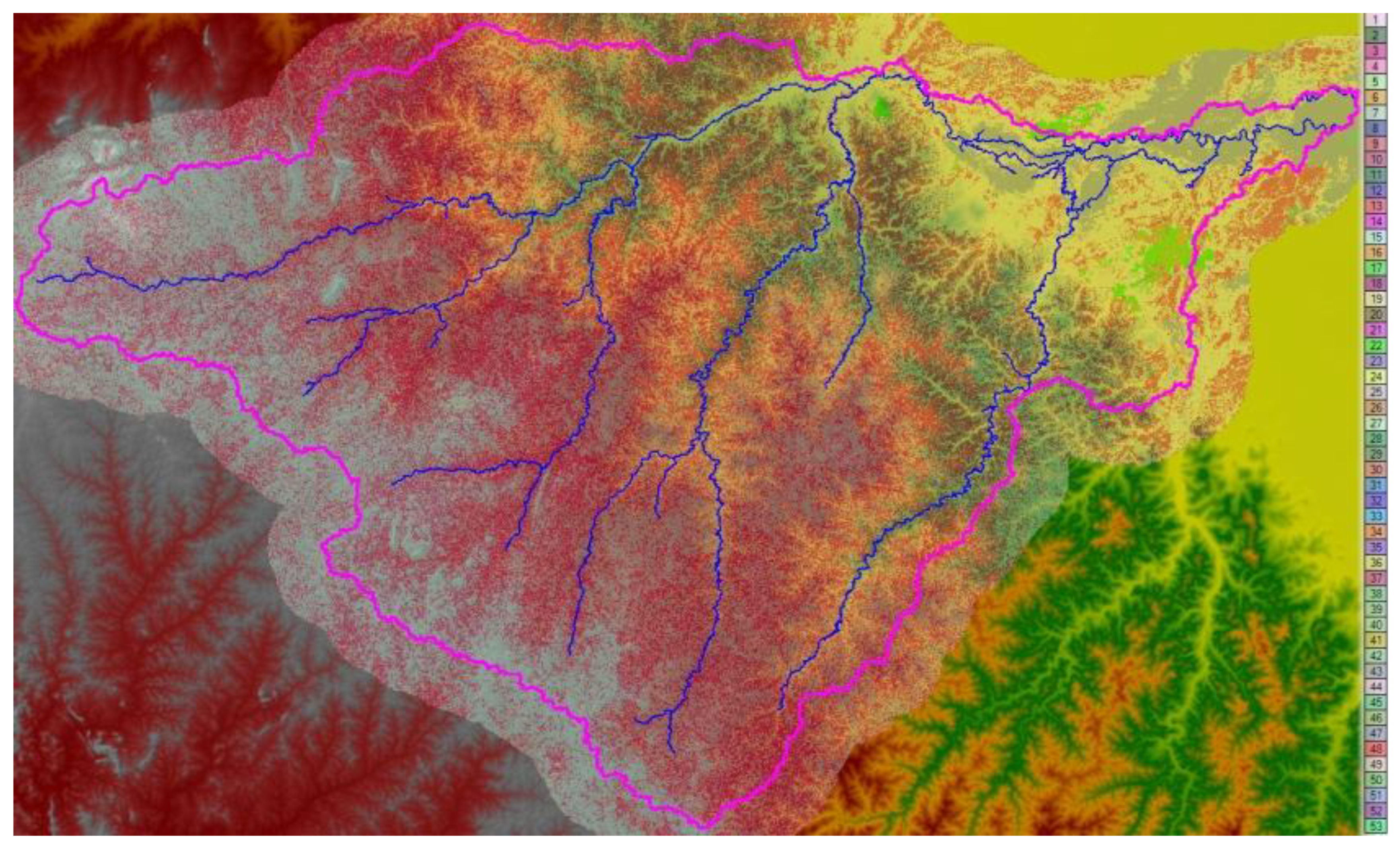
Infiltration
The infiltration map layer was then loaded (Figure 15)
Figure 15.
Infiltration parameters.
Modelling Results for Catchment Covering Projects in Aweil South
Flood Hydrograph at Outlet of Catchment
From the flood hydrograph (Figure 16) derived for the boundary condition (BC) line at the outlet of the catchment the peak was found to be 2,093.748 m³/s which occurred on 31st August 2024.
Figure 16.
Flood hydrograph at outlet of catchment.
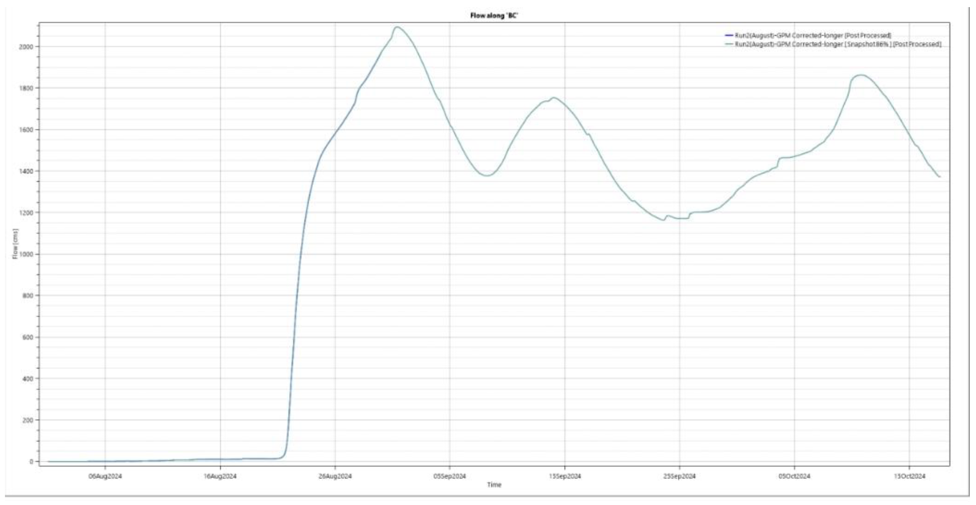
illustrates the variation in discharge over time during a flood event at the catchment’s outlet. The hydrograph typically features a sharp rising limb, indicating rapid runoff following intense rainfall, followed by a peak discharge point that represents the maximum flow rate. After the peak, the falling limb shows a gradual decline in discharge as the floodwaters recede
Water Surface Elevations
Figure 17.
Water surface elevations.
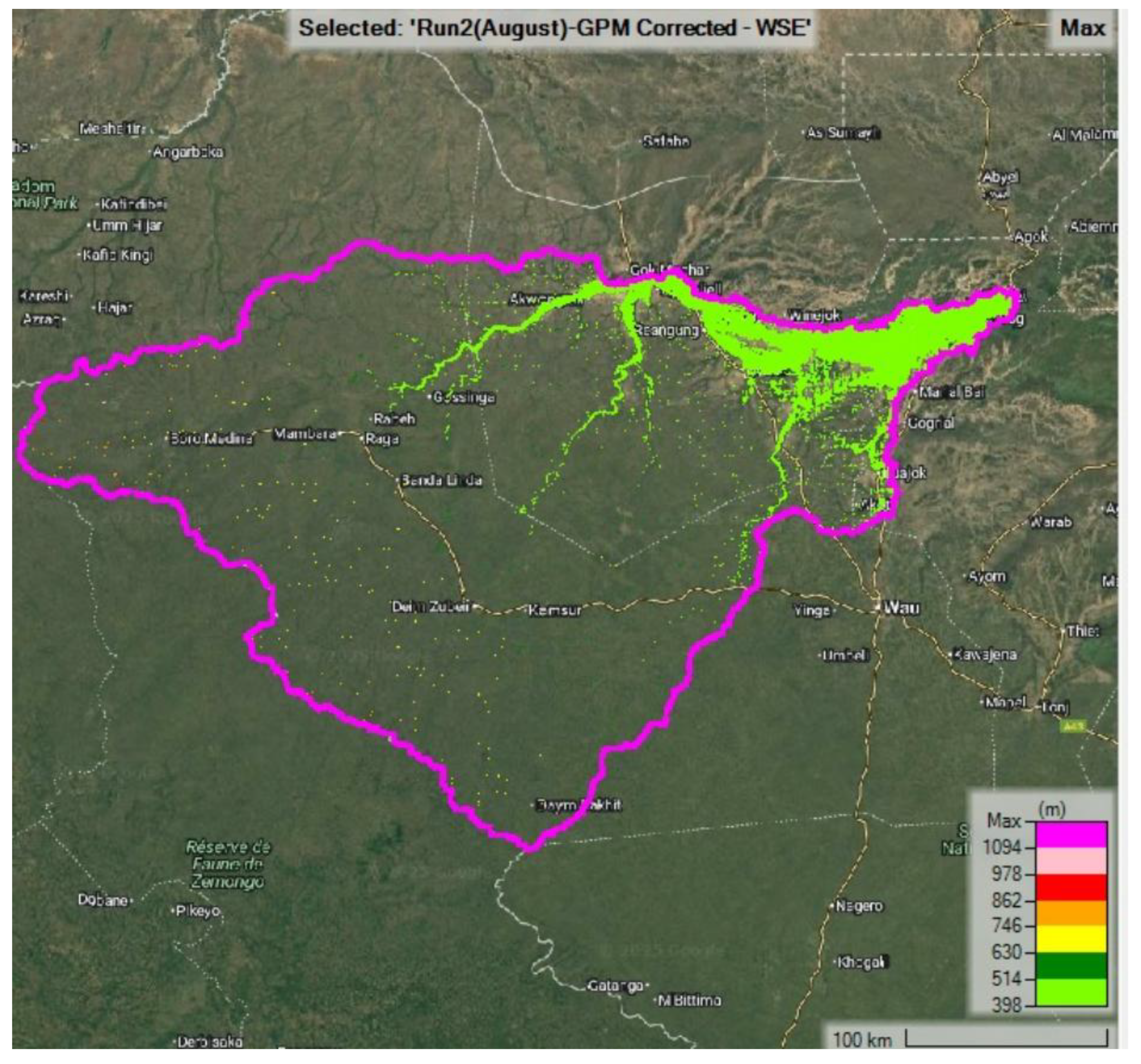
With the month of August experiencing the greatest magnitude of rainfall, the water surface elevations(Figure 17) are generally high upto almost 750 masl especially along and adjacent to the rivers. The area from Gok Machar through Aweil towards the outlet of the catchment is now one big sea.
Water Depths
Figure 18.
Water depths.
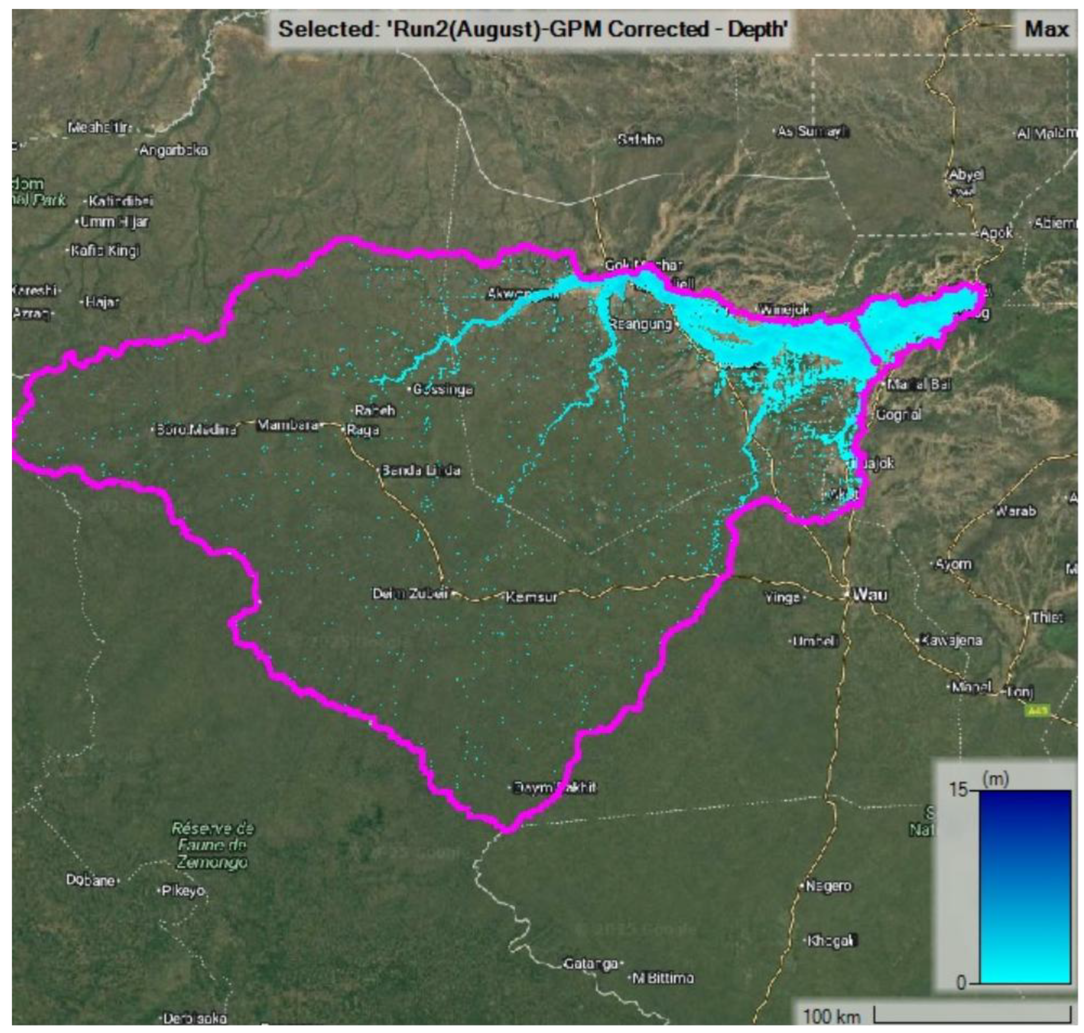
Water depths (Figure 18) increase even upto 5m especially in river channels, in the month of August.
Water Velocity
Figure 19.
Water velocity.
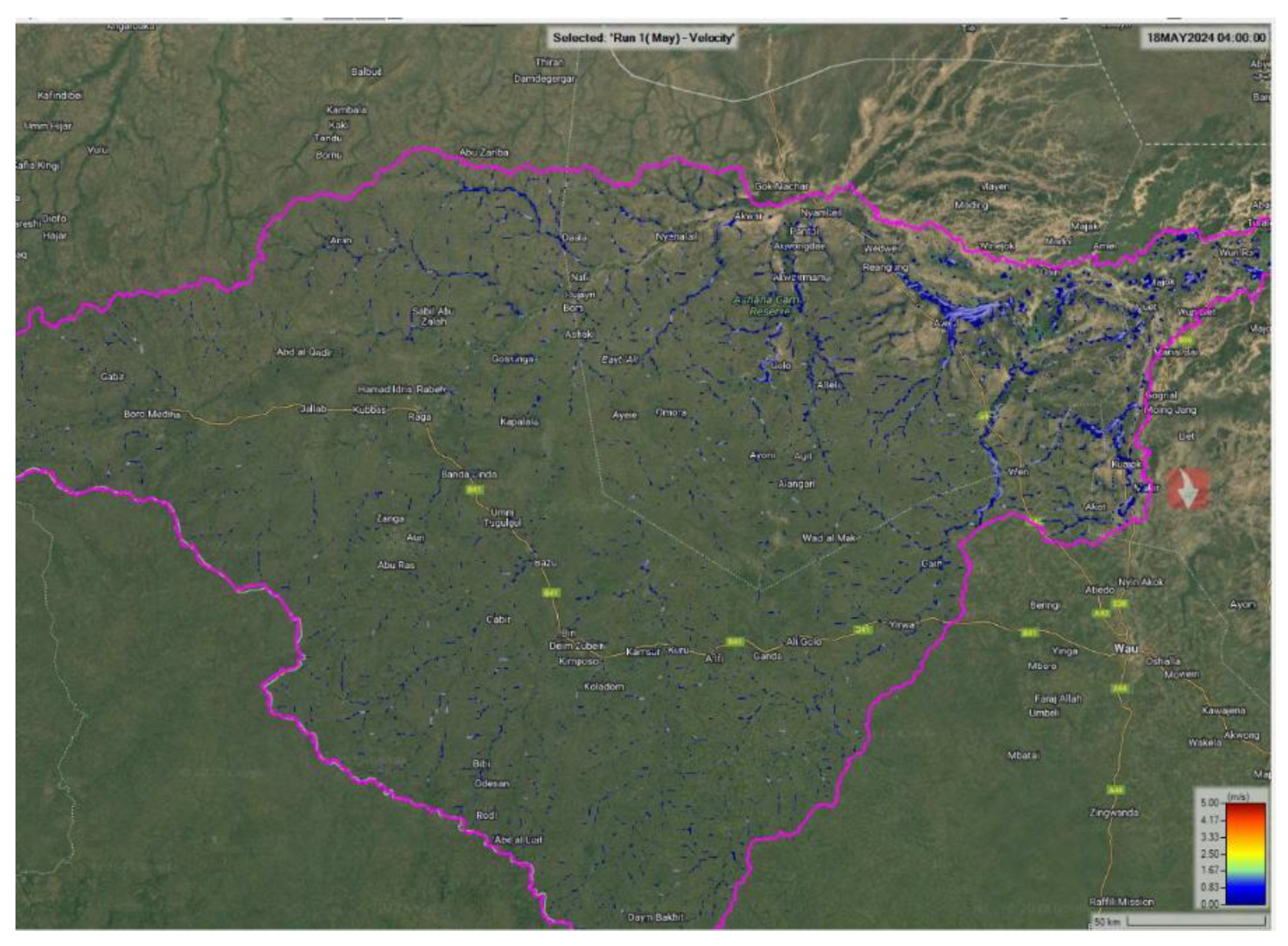
The floods in August are swift, generally, dispersed and shallow, at the sources getting even stronger and hazardous downstream of Wedwell and Aweil going to about 1.5m/s.
Flood Hazard ARR Map
Flood Hazard Categories
The actual hazard posed by floodwaters to objects such as houses, vehicles, and people depends on a combination of two key factors: water depth and flow velocity. Each object has its own specific vulnerability to this combination, which determines the level of risk during a flood event. Extensive studies have been conducted to quantify these risks, particularly for residential structures, automobiles, and human safety. These findings have been consolidated into the Australian Rainfall and Runoff Guidelines hazard categories, which provide a standardized framework for assessing flood hazards (ARR Guidelines).
This classification is visually represented in Figure 20, which illustrates the hazard categories based on model results for both catchments. The figure highlights zones of varying risk levels, helping to identify areas where floodwaters pose significant threats to life and property. This approach supports informed decision-making in floodplain management, emergency planning, and infrastructure design.
Figure 20.
ARR Combined Flood Hazard Curves (Smith, Bustamante et al. 2014).
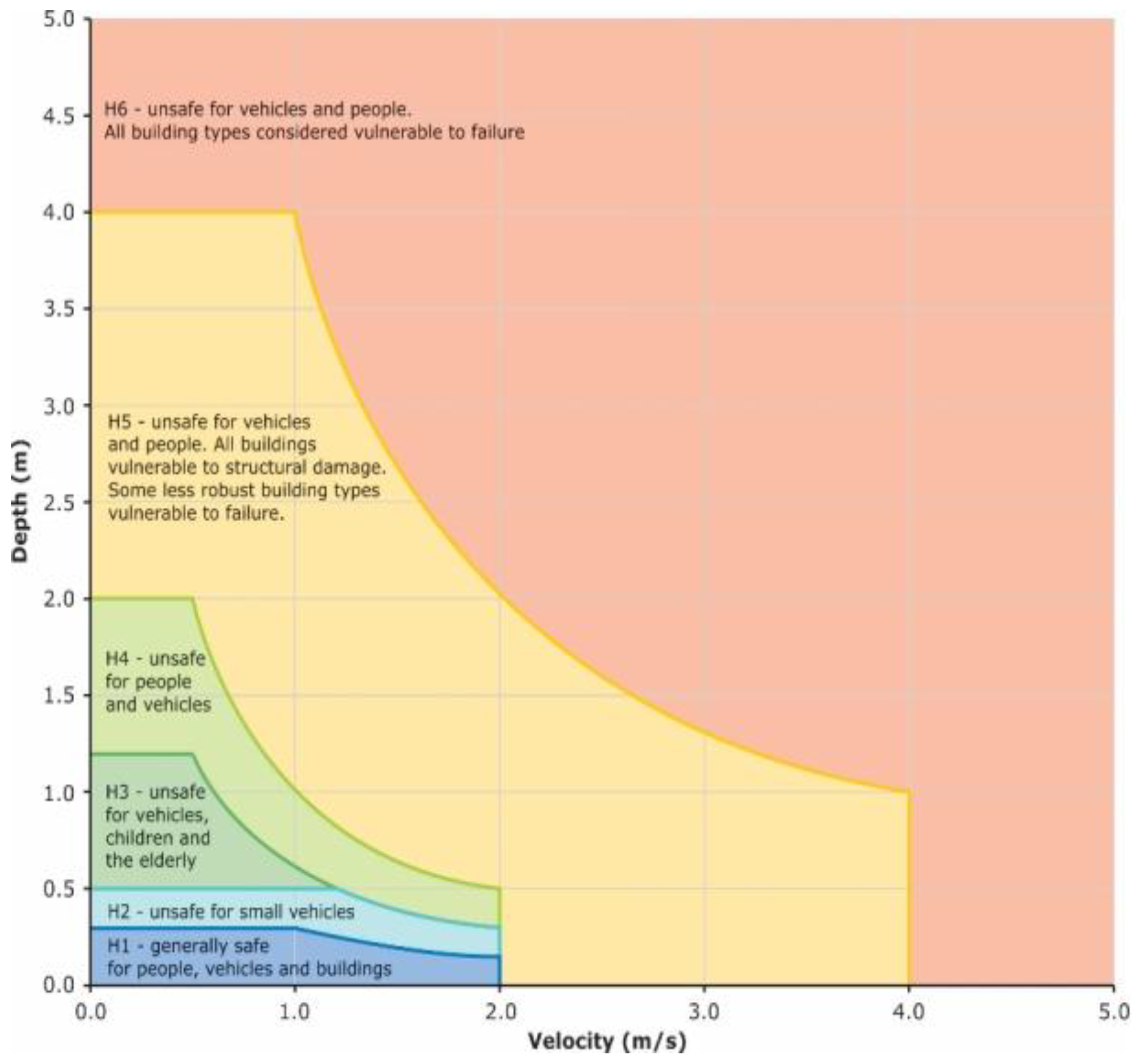
Figure 21.
Flood hazard map.
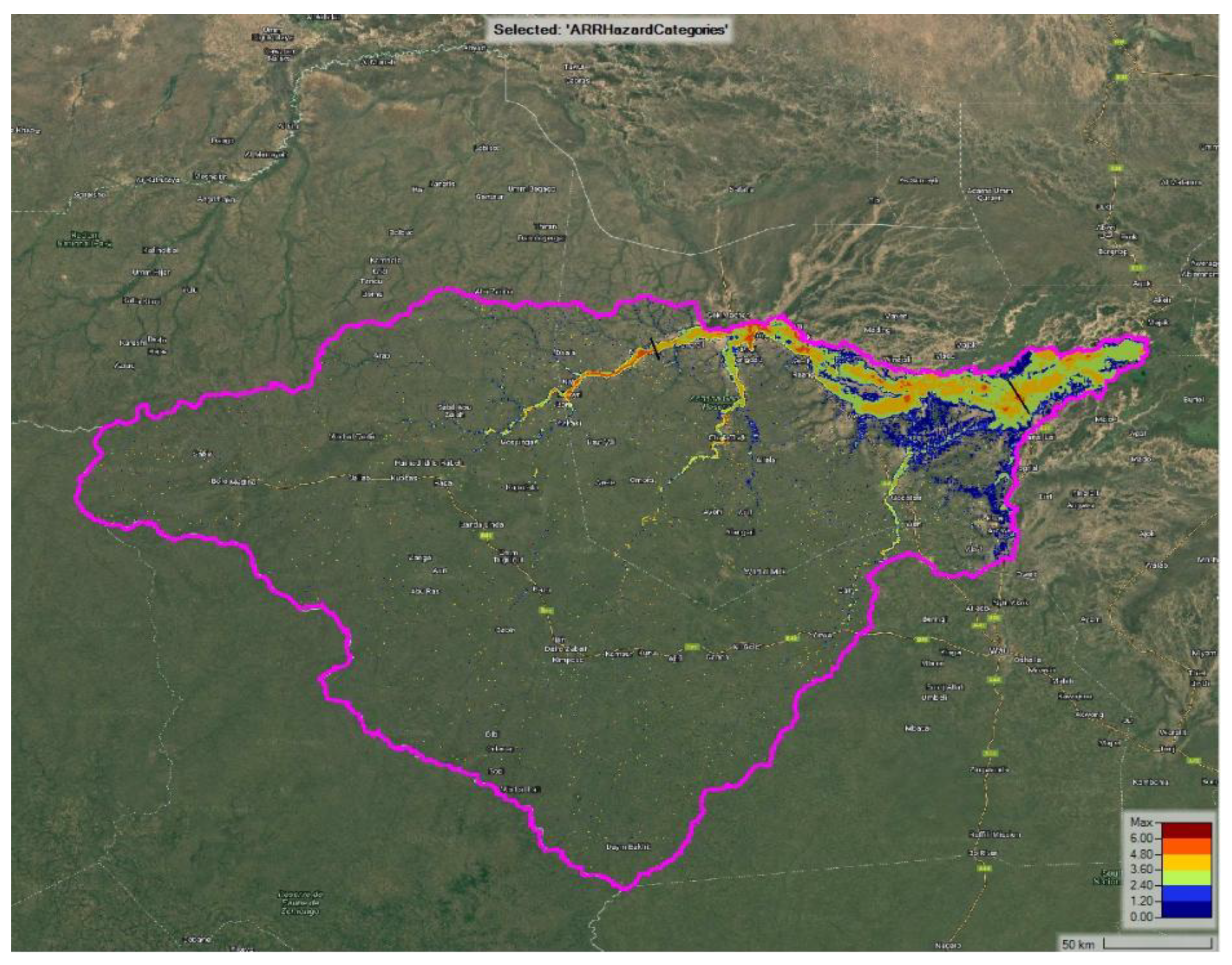
Based on the flood hazard categorization described above, the majority of the river floodplain falls within Category 3, indicating moderate hazard levels. In certain areas, particularly along the main channel, localized zones exhibit Category 4 and 5 hazards, reflecting high to very high risk. South of this floodplain zone, hazard levels decrease significantly, with most areas classified as Category 2 or lower, suggesting relatively low flood risk.
Conclusion
This study applied a geospatial and hydrological modeling approach to assess flood patterns in Aweil East and South, South Sudan. Using HEC-RAS Rain-on-Grid simulations, rainfall frequency analysis, and land cover classification, the research quantified runoff volumes and identified flood-prone zones across low-gradient terrain. A weighted Curve Number of 87.2 was derived from satellite-based land use data, enabling accurate runoff estimation. The results revealed that even frequent rainfall events with 1–2 year return periods can generate significant flood hazards, particularly in areas with poor drainage and minimal elevation change. Flood hazard categorization showed that most of the river floodplain falls within Category 3, with localized zones reaching Category 4 and 5, indicating high risk to settlements and infrastructure.
Recommendations
- Floodplain Zoning: Implement land use planning and zoning regulations to restrict development in high-hazard floodplain areas, especially those classified under Categories 4 and 5.
- Early Warning Systems: Establish community-based flood monitoring and early warning systems to improve preparedness and reduce vulnerability.
- Infrastructure Design: Adapt rural infrastructure—such as roads, culverts, and housing—to withstand frequent flooding, using hazard maps to guide resilient design.
- Wetland Conservation: Protect and restore natural wetlands and depressions that serve as flood buffers, enhancing the landscape’s capacity to absorb runoff.
- Further Research: Conduct long-term hydrological monitoring and expand modeling to include climate change scenarios, ensuring adaptive flood risk management.
References
- FABDEM Website (https://data.bris.ac.uk/data/dataset/s5hqmjcdj8yo2ibzi9b4ew3sn).
- The data can be accessed from the FABDEM Website (https://data.bris.ac.uk/data/dataset/s5hqmjcdj8yo2ibzi9b4ew3sn.
- Ba, N. S., A. Usman, A. Gasasira, P. Kabore, B. Achu, H. Kulausa, E. Chanda, O. O. Olu, J. Cabore and M. Moeti (2025). “Transforming technical assistance for more effective health services delivery in Africa: the WHO multi-country assignment teams experience.” Frontiers in Public Health 13: 1560361. [CrossRef]
- Batjes, N. H. (2022). “Overview of procedures and standards in use at ISRIC WDC-Soils (ver. 2022).”.
- Batjes, N. H., L. Calisto and L. M. de Sousa (2024). “Providing quality-assessed and standardised soil data to support global mapping and modelling (WoSIS snapshot 2023).” Earth System Science Data 16(10): 4735-4765. [CrossRef]
- Du, H., M. L. Tan, F. Zhang, K. P. Chun, L. Li and M. H. Kabir (2024). “Evaluating the effectiveness of CHIRPS data for hydroclimatic studies.” Theoretical and Applied Climatology 155(3): 1519-1539. [CrossRef]
- Gakai, P. K., R. K. Waweru, A. Mutisya and N. Mukami (2025). “Flood Impacts on Vulnerable Communities in Aweil East and South: A Qualitative Assessment.”.
- Gakai, P. K., R. K. Waweru, A. Mutisya, K. NM and V. K. Kimathi (2025). “Inclusive Recovery in Aweil East and South: A Social Baseline for Equity and Resilience.” Preprints, Preprints.
- Gibbs, D. A., M. Rose, G. Grassi, J. Melo, S. Rossi, V. Heinrich and N. L. Harris (2025). “Revised and updated geospatial monitoring of 21st century forest carbon fluxes.” Earth System Science Data 17(3): 1217-1243. [CrossRef]
- Hawker, L., P. Uhe, L. Paulo, J. Sosa, J. Savage, C. Sampson and J. Neal (2022). “A 30 m global map of elevation with forests and buildings removed.” Environmental Research Letters 17(2): 024016. [CrossRef]
- Kipkemoi, I., G. K. Sitati and P. K. Gakai (2025). “Exploring the impact of sister city partnerships on emerging African cities.” Discover Cities 2(1): 1-17.
- Lai, C., M. Xie and D. Murthy (2003). “A modified Weibull distribution.” IEEE Transactions on reliability 52(1): 33-37.
- Meng, J., Z. Dong, G. Fu, S. Zhu, Y. Shao, S. Wu and Z. Li (2024). “Spatial and Temporal Evolution of Precipitation in the Bahr el Ghazal River Basin, Africa.” Remote Sensing 16(9): 1638. [CrossRef]
- Onyutha, C., H. Tabari, M. T. Taye, G. N. Nyandwaro and P. Willems (2016). “Analyses of rainfall trends in the Nile River Basin.” Journal of hydro-environment research 13: 36-51. [CrossRef]
- Smith, P., M. Bustamante, H. Ahammad, H. Clark, H. Dong, E. A. Elsiddig, H. Haberl, R. Harper, J. House and M. Jafari (2014). Agriculture, forestry and other land use (AFOLU). Climate change 2014: mitigation of climate change. Contribution of Working Group III to the Fifth Assessment Report of the Intergovernmental Panel on Climate Change, Cambridge University Press: 811-922.
- Wanjiru, M. C., N. M. Kathuri, N. A. Mutio and P. K. Gakai (2025). “Determinants of Energy and Water Source Choices in Secondary Schools in Mbeere South Sub-County, Kenya: A Resource Dependence Perspective.”.
Disclaimer/Publisher’s Note: The statements, opinions and data contained in all publications are solely those of the individual author(s) and contributor(s) and not of MDPI and/or the editor(s). MDPI and/or the editor(s) disclaim responsibility for any injury to people or property resulting from any ideas, methods, instructions or products referred to in the content. |
© 2025 by the authors. Licensee MDPI, Basel, Switzerland. This article is an open access article distributed under the terms and conditions of the Creative Commons Attribution (CC BY) license (http://creativecommons.org/licenses/by/4.0/).
Copyright: This open access article is published under a Creative Commons CC BY 4.0 license, which permit the free download, distribution, and reuse, provided that the author and preprint are cited in any reuse.


