
Submitted:
14 September 2025
Posted:
15 September 2025
You are already at the latest version
Abstract
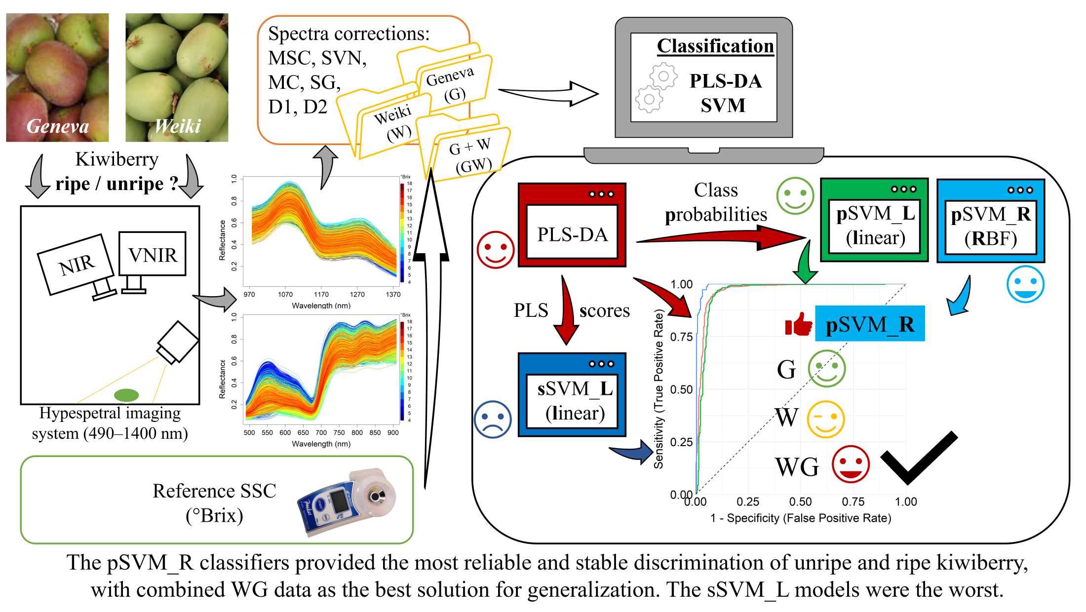
The accurate and non-destructive assessment of fruit ripeness is essential for post-harvest sorting and quality management. This study evaluated a meta-inspired classification framework integrating partial least squares discriminant analysis (PLS-DA) with support vector machines (SVMs) trained on latent variables (sSVM) or on class probabilities (pSVM) derived from multiple PLS-DA components. Two kiwi-berry varieties, ‘Geneva’ and ‘Weiki’, were analyzed using variety-specific and combined datasets. Performance was assessed in calibration and prediction using accuracy, F05, Cohen’s kappa, precision, sensitivity, specificity, and likelihood ratios. Conventional PLS-DA provided reasonably good classification, but pSVM models, particularly those with an RBF kernel (pSVM_R), consistently outperformed other approaches and ensured higher stability across all datasets. Unlike sSVMs, which were prone to over-fitting, pSVM_R models achieved the highest accuracy of 92.4–96.9%, Cohen’s kappa of 84.8–93.9%, and precision of 89.1–94.2%, clearly surpassing both score-based SVM and PLS-DA. Contrasting tendencies were observed between cultivars: ‘Geneva’ models improved during prediction, while ‘Weiki’ models declined, especially in specificity. Combined datasets provided greater stability but slightly reduced peak performance than single-variety models. These findings highlight the value of probability-enriched stacking models for non-invasive ripeness discrimination, suggesting that adaptive or hybrid strategies may further enhance generalization across diverse cultivars.
Keywords:
classification
; kiwiberry
; hyperspectral imaging
; machine learning
; PLS-DA
; sorting system
; SVM
1. Introduction
Actinidia arguta (Siebold et Zucc.) Planch. ex Miq., commonly referred to as kiwiberry or minikiwi, is a climacteric fruit valued for its exceptional sensory and nutritional properties [1,2,3,4]. It is particularly rich in vitamin C, polyphenols, carotenoids, and other bioactive compounds that contribute to its classification as a “superfruit” [5,6]. In Poland, commercial cultivation has developed over the last 25 years, with varieties such as ‘Weiki’, ‘Geneva’, and ‘Bingo’ gaining the greatest importance [4,7].
Despite its potential, kiwiberry remains a commercially challenging fruit. Its short storage life, high susceptibility to uneven ripening, and seasonal availability limit market expansion and profitability [8,9]. In the Polish climate, fruits are typically harvested at the stage of harvest maturity, when they are still firm and sour, and then undergo rapid and heterogeneous ripening after harvest [10]. This variability makes post-harvest sorting according to ripeness a key step for extending market supply, reducing losses, and ensuring uniform fruit quality.
Traditional assessment of soluble solids content (SSC), the main ripeness indicator in Actinidia spp., relies on destructive refractometric measurements [11,12,13]. Therefore, non-destructive technologies are required for practical implementation on sorting lines. This requirement can be successfully met by solutions based on vision techniques, particularly hyperspectral imaging, which has proven to be an effective quality control tool, integrating spectral and spatial information for the rapid and non-invasive assessment of examined objects. Recent studies have demonstrated the effectiveness of HSI in predicting the quality of Actinidia ssp., including their health [14,15,16], texture [17,18], maturity [19,20,21,22], soluble solid content and acidity [23,24,25], or storage condition [26,27].
For modelling of spectral data, whether in classification or regression tasks, partial least squares (PLS) method and its variant, PLS discriminant analysis (PLS-DA), have been widely applied, offering both dimensionality reduction and interpretable class separation [20,28]. Analogous to their long-standing role in chemometrics both approaches are increasingly used for quantitative information extracted from hyperspectral images, where spectral variables exhibit high collinearity and redundancy [29]. Such strategies not only facilitate the interpretation of spectral signatures but also provide a structured basis for integrating machine learning algorithms that further enhance predictive performance.
PLS-DA is a variant of linear regression using the same method as PLS-R, developed as an alternative to principal component regression (PCR). It is beneficial when explanatory variables are highly correlated and far outnumber the observations. PLS-R combines modeling of relationships between explanatory and response variables with dimension reduction, replacing the original variables with a smaller set of orthogonal latent variables (factors or components). This approach overcomes the limitations of classical regression in cases of strong multicollinearity. Unlike PCR, PLS-R projects factors by accounting for the variance of both explanatory and response variables. PLS-DA adapts PLS-R to classification tasks, where the response variable is nominal and must be encoded with c or c–1 dummy variables. The procedure is thus performed with multiple dependent variables, each estimated separately. The resulting set of quantitative outputs, one for each dummy variable, forms the basis of the classification rule. The optimal number of factors is selected to minimize classification error, typically estimated by cross-validation. Unlike linear discriminant analysis (LDA), PLS-DA does not derive discriminant functions. Objects are instead assigned to the class whose dummy variable attains the highest value [30,31,32,33].
On the other hand, the high dimensionality and collinearity of spectral data encourage the use of advanced machine learning algorithms, including neural networks, particularly convolutional architectures, as well as automated variable selection techniques such as CARS — competitive adaptive reweighted sampling [21,34], BoSS — Bootstrapping soft shrinkage [24], GA — genetic algorithms [35,36], VIP — variable importance in projection [20] , or SPA — successive projections algorithm [19]. A practical advantage lies in approaches that either automatically reduce the number of variables based on their contribution to predictive accuracy or handle nonlinear relationships more effectively than traditional statistical models. Within this context, support vector machines (SVM) provide a powerful alternative, offering strong generalization capabilities in high-dimensional feature spaces and demonstrating robustness when combined with tailored kernel functions. SVM method can be applied to regression and classification tasks. It enables the construction of nonlinear decision boundaries through various kernel functions, if defining a linear boundary between classes is difficult. This mechanism, known as the kernel trick, maps the original n-dimensional data into a new mathematical space, usually of higher dimensionality, where the decision boundary is determined based on the observations closest to it. These observations, referred to as support vectors, define the boundary as their linear combination [37]. The most common kernels include linear, radial basis function (RBF), sigmoid, and polynomial. The margin is the distance between observations belonging to different classes and lying on opposite sides of the boundary. A wider margin improves the model’s generalization ability and is therefore maximized during training [38]. Perfect separation is rarely achievable, regardless of the kernel, because class boundaries often overlap. This issue is addressed by allowing some observations to fall on the wrong side of the boundary. The trade-off between the number of such misclassified observations and the margin width is controlled by the C parameter, which introduces additional constraints into the SVM optimization function. A low C prioritizes margin width over classification errors, while a high C reduces tolerance for misclassified observations. Alongside kernel-specific parameters, C is optimized in every SVM model [39]. SVM is a promising solution, effective in handling non-linear decision boundaries and often provide superior classification or prediction accuracy in hyperspectral applications [25,40,41]. Stacking or meta-learning approaches that combine SVM and feature extraction models may further enhance robustness and predictive performance, offering a promising direction for ripeness-based sorting of kiwiberry.
While hyperspectral imaging has been widely explored for fruit quality evaluation, the choice and design of classification strategies remain critical for practical implementation. Previous studies often rely on single classifiers or raw spectral inputs, overlooking the potential of combining feature extraction with robust machine learning models. This study addresses this gap by systematically comparing PLS-DA, SVM with different kernels, and hybrid SVM-PLS approaches, providing insights into their relative performance and suitability for automated kiwiberry sorting. Notably, PLS-based methods are particularly well-suited for high-dimensional data typical of hyperspectral analyses, where the number of predictors substantially exceeds the number of observations. In this context, hyperspectral imaging does not precisely quantify individual chemical constituents, but captures spectral patterns that enable object classification, grouping, and similarity assessment in post-harvest sorting processes.
Therefore, this study aimed to evaluate a meta-inspired classification framework combining multiple modeling strategies to classify kiwiberry fruits according to their ripeness. Specifically, we compared classical PLS-DA, SVM models trained on latent variables extracted from PLS-DA (sSVM), and SVM models leveraging class probabilities (pSVM) derived from multiple PLS-DA models with varying numbers of components, each validated by random 10-fold cross-validation. This approach enabled a systematic assessment of the potential of integrating hyperspectral imaging with advanced classification techniques for optimized post-harvest fruit sorting. pSVMs may be considered stuck models, since they rely directly on the original feature space and are constrained by the geometry of the raw predictors, while sSVMs operate in a transformed latent space derived from PLS-DA scores, which changes the numerical nature of the optimization problem and alters the generalization behavior. The study underscores the importance of model architecture and feature extraction in advancing non-invasive post-harvest fruit sorting systems.
2. Materials and Methods
2.1. Collection and Preparation of Kiwiberry Samples
The fruits of A. arguta represent two varieties, ‘Weiki’ and ‘Geneva’, which were used to develop classifiers. Fruits originated from a commercial plantation in Bodzew, along Grójec, Mazowieckie voivodship, Poland (51°47’50’’N, 20°48’43’’E; USDA hardiness zone 6b). Harvests were carried out in 2021 and 2022 in early September. Fruits were collected randomly at the harvest maturity stage, with an SSC of 6.5–7% [8,9]. Fruits were kept at 1° C and 90% relative humidity and monitored for up to several days to capture ripeness variations, beginning on the day of harvest. From this batch 5,938 samples were chosen randomly and employed for model development, comprising 3,810 ‘Weiki’ fruits and 2,128 ‘Geneva’ fruits, the latter of which were collected exclusively in 2022. The experimental protocol, including fruit storage, initial sample preparation, acquisition and preliminary processing of hyperspectral images, and measurement of fruit extract, was identical in both study years and similar to those described by Janaszek-Mańkowska & Ratajski [42].
2.2. Hyperspectral Imaging Setup
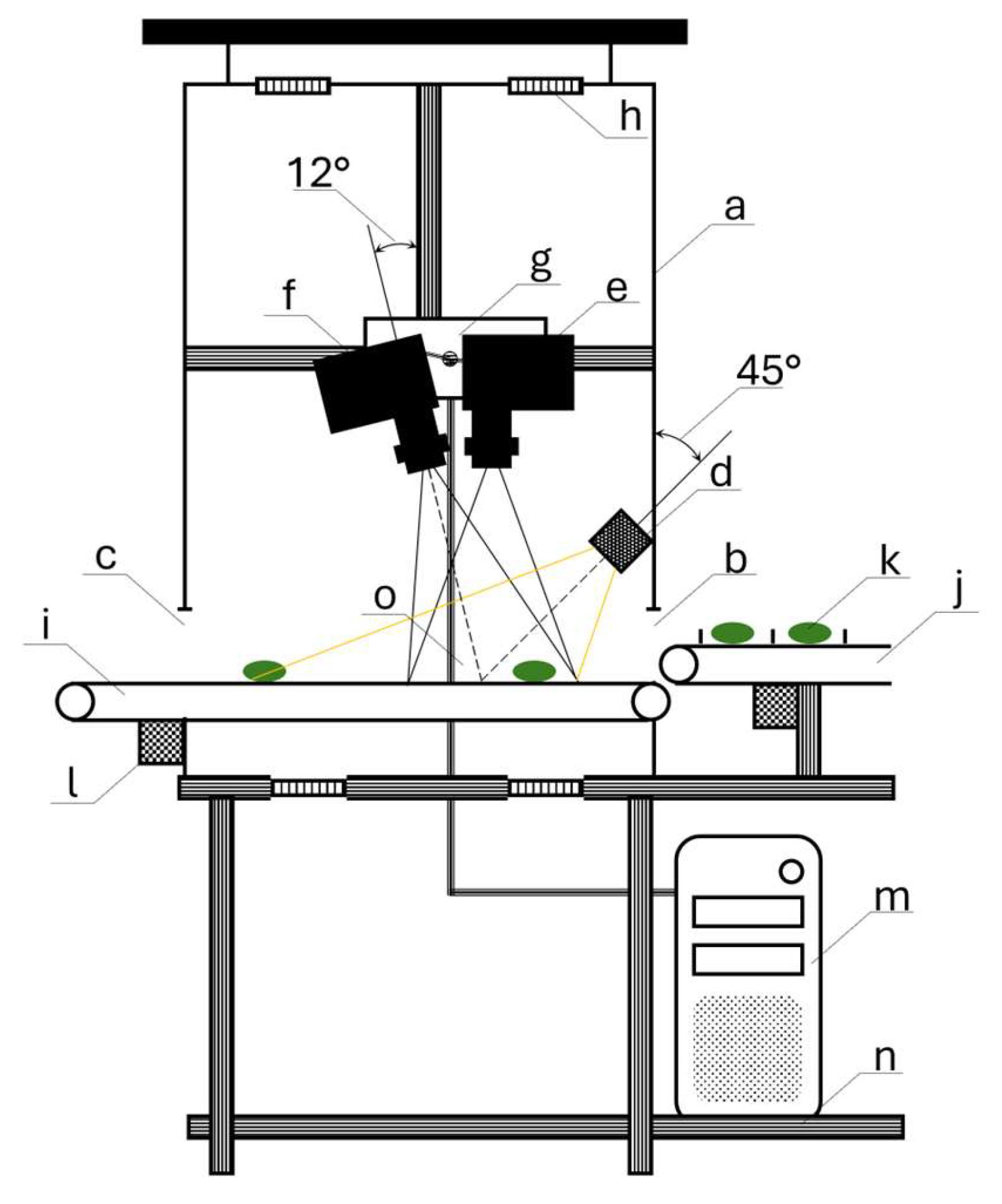
The hyperspectral imaging setup (HIS) employed a push-broom line scanning technique and consisted of two hyperspectral cameras, FX10 (CMOS detector) and FX17 (cooled InGaAs detector) from SPECIM Ltd. (Oulu, Finland), a 250 W halogen lamp, and an external PC. The FX10 camera operated in the 400–1000 nm range (visable-near infrared, VNIR) with 448 spectral bands, while the FX17 covered 900–1700 nm (short-wave infrared, SWIR) with 224 bands. To reduce external light interference, all HIS components except the PC were enclosed in a vision chamber which was the core of the prototype kiwiberry sorting device and consisted also forced air exhaust system and four transducers (F&F, model MB-AHT-1) connected to a PLC (Siemens, S7-1214C) to monitor and prevent overheating from the halogen lamp. Both cameras were placed above a conveyor belt, moving randomly positioned fruits at 40 mm/s. The optical axis of FX10 was perpendicular to the conveyor, while FX17 was tilted ~12° to capture the same sample area. The halogen lamp was positioned at a 45° angle. Both cameras acquired 12-bit images with mean spectral resolutions of 1.32 nm (FX10) and 3.57 nm (FX17).
Figure 1.
Vision chamber with equipment (part of a prototype device for sorting kiwiberry fruits): a – chamber housing, b – inlet, c – outlet, d – 250 W halogen lamp, e – FX10 camera, f – FX17 camera, g – mounting plate, h – fan, i – belt conveyor, j – carrier conveyor (fragment), k – kiwiberry, l – electric motor driving the conveyor, m – PC computer, n – support frame element, o – Camera Link data transmission cable.
2.3. Processing Workflow for Hyperspectral Reflectance Data
The OpenCV custom application supported the automatic acquisition of hyperspectral cubes of each fruit and further image pre-processing. In order to correct for spectral light variations, sensor sensitivity, and dark current, radiometric calibration was performed using dark and white reference images (0% and 99% reflectance, respectively) as proposed by Xiong, et al. [43]:
where IC and IO are the calibrated and original images, ID is the dark reference (camera shutter closed, light off), and IW is the white reference (PTFE tile imaged before each cycle under the same light conditions as IO).
Each hypercube was sliced into 16-bit 2D images, representing reflectance in individual spectral bands. Although hyperspectral images initially covered the full ranges recorded by both cameras, bands with low signal-to-noise ratio (SNR), poor discriminative capacity, observed mainly at the ends of the SWIR range, or redundancy due to spectral overlap were discarded after preliminary inspection. Only bands within ~490–909 nm and ~977–1379 nm were retained for further analyses. In the sequence of selected 2D images corresponding to each fruit, a region of interest (ROI) was defined to include only the fruit, and subsequent image processing steps were applied exclusively within this ROI. At the same time, the remaining background was excluded from analysis. ROI location, which covered the entire fruit surface, was specified separately for VNIR and SWIR image sequences using the IsoData binary threshold [44] on hypercube slices with the highest contrast between background and sample reflectance. For each waveband λ, the mean reflectance within the ROI was calculated according to the formula (2):
where is the mean reflectance within the ROI for a given wavelength λ, Rp is the reflectance of the n-th pixel, and n is the total number of pixels.
Although calibration reduces many artifacts, spectral data can still be affected by baseline drift, nonlinearity, or scattering effects, which introduce noise unrelated to the actual signal. Several pre-processing techniques were applied separately to the VNIR and SWIR ranges to address these disadvantages. These included Multiplicative Scatter Correction (MSC), Standard Normal Variate (SNV), Savitzky–Golay (SG) smoothing, mean centering (MC), and spectral derivatives of the first (D1) and the second order (D2). For SG filtering, a frame size of 15 was used, corresponding to bandwidths of 18.56 nm (VNIR) and 48.52 nm (SWIR). Derivatives, calculated after SG smoothing with low-order polynomial fitting, were used to reduce baseline and slope effects while improving the resolution of overlapping features. MSC compensated for scatter by aligning spectra with a reference [45,46], whereas SNV normalized each spectrum relative to its mean and standard deviation [47]. MC emphasized spectral variation by shifting each spectrum relative to the overall average. SG filtering smoothed the signal through polynomial convolution [48]. Derivatives further corrected baseline and slope shifts, though smoothing was essential to limit noise amplification [46,49]. All these corrections were implemented in R using the mdatools package [50,51].
2.4. Determination of SSC as a Ripeness Index
SSC served as the reference index of kiwiberry ripeness. Following hyperspectral image acquisition, fruit juice was extracted and analyzed with a digital refractometer (ATAGO, PAL-1, Tokyo, Japan), providing ±0.1% accuracy within the 0–53 °Brix range. Measured SSC values spanned from 4.4% to 17.1% (mean 8.02 ±2.5%) for ‘Weiki’ fruits and from 4.3% to 13.6% (mean 7.82 ±1.7%) for ‘Geneva’ fruits, thus covering a broad maturity spectrum, including levels exceeding commercial standards.
2.5. Data Preparation
Data obtained from hyperspectral images were organized into datasets corresponding to the kiwiberry variety. Class of fruit ripeness was defined based on SSC so that samples with SSC ≤ 7% were assigned to the unripe class (A — positive class), whereas the remaining fruits were classified as ripe (B — negative class). The class label was treated as the dependent variable, while the predictor set comprised 425 spectral variables, including 309 wavebands from the VNIR range and 116 from the SWIR range. Three datasets were prepared: (i) ‘Weiki’ variety data (W) from two harvest years, (ii) ‘Geneva’ variety data (G), and (iii) a combined dataset including both ‘Geneva’ and ‘Weiki’ varieties (WG). Each dataset was split into training and test subsets in a 4:1 ratio (80% training, 20% test). The training part was used to calibrate classification models, while the independent test set served as external validation of model performance. Stratified random sampling was performed with the createDataPartition function from the caret package [52] ensuring balanced class proportions in training and test subsets. Model calibration relied on training datasets (with internal cross-validation applied during training), whereas test data were used for prediction. In this context, ‘calibration’ refers to model optimization and evaluation based on cross-validated training results, while ‘prediction’ denotes the assessment of the final model on the independent test set. Detailed information on datasets structure are summarized in Table 1.
Following the data partition, spectral preprocessing (MSC, SNV, SG, MC, D1, D2) was applied, yielding 18 training — test set pairs for subsequent analyses. Preprocessing was done separately for training and test subsets to avoid data leakage.
2.6. PLS-DA & SVM Classification
Classification models were implemented in the caret package, which applied the pls package for PLS-DA [53] and the kernlab library for SVM [54,55]. Model calibration was consistently performed using random 10-fold cross-validation on the training set to prevent overfitting. The modeling procedure consisted of two main stages. First, PLS-DA was employed to obtain independent classifiers, which also served as a Level-0 models to provide a set of latent variables (scores) as well as winning class probabilities for subsequent Level-1 SVM models developed in the second stage. The idea of Level-0 and Level-1 generalizers is given in [56]. The optimal number of PLS components in each model was determined based on the kappa statistic [57], defined as:
where po, which denotes the observed agreement (proportion of correctly classified samples), is given as:
and pe denotes the expected agreement by chance, calculated from the marginal distributions of the confusion matrix as follows:
where TPi, FPi, and FNi denote the elements of the confusion matrix shown in Table 2 for class i, and n is the total number of observations.
Table 2 presents a confusion matrix for binary classification with positive class A (unripe fruits) and negative class B (ripe fruits), where TP and TN denote the number of correctly classified samples, whereas FP and FN indicate the number of misclassifications [58].
The optimal number of PLS components typically amounted to 18 or 20, indicating relatively high model complexity. Thus, for subsequent analyses with SVM classifiers based on scores (sSVM), the maximum number of latent variables extracted from the training set was capped at 20, and test set scores were calculated using the corresponding loading weights, ensuring that both datasets were represented in the same latent space. Thereby, the dimensionality of the input space was reduced from 425 original spectral variables to 20 scaled and transformed latent predictors. Moreover, considering the most common optimal number of latent variables (20), an additional 18 alternative and independent PLS-DA models were fitted, with the number of components increased stepwise by one, starting from 3. For each PLS-DA model, class probabilities for the winning class (class A) were computed separately for the training and test sets. The probabilities derived from the training set were subsequently used as predictors in SVM models (pSVM), whereas those obtained from the test set were retained exclusively for their independent validation. Therefore, pSVMs may be considered stacked models similar to description by Ting & Witten [56], as they operated on meta-level inputs rather than raw or transformed predictors. By contrast, sSVMs relied directly on latent variables, linear combinations of the original spectral features.
In the second stage, SVM classifiers with linear (SVM_L) and radial (RBF) kernels (SVM_R) were developed, but the latter were used only with pSVM variants. This decision was based on the linear nature of the latent variables, which are constructed to maximize class separation. Introducing a nonlinear kernel would likely add complexity without improving separability, as linear boundaries are already sufficient in the latent space [59]. While the behavior of RBF kernels in this context is of academic interest, their inclusion was deemed unnecessary for practical model development. For SVM_L models, the regularization parameter C was optimized, whereas for SVM_R models, both C and γ (the kernel width parameter) were tuned. Parameter optimization was done by exhaustive grid search to maximize the κ statistic in a random 10-fold cross-validation. Based on the provided training data, candidate grids were generated automatically using 20 values for each parameter. The selection of components in sSVM_L models was constrained to sequential combinations (e.g., 1–3 or 1–5), while irregular patterns (1, 4, 8) were excluded. Our decision was motivated by the inherent structure of PLS components, where successive latent variables explain progressively smaller portions of the shared variance, and skipping intermediate components would lead to less coherent models.
2.7. Evaluation of Classification Performance
Standard classification metrics, such as accuracy (ACC), sensitivity (TPR), specificity (TNR), precision (PPV), the F05 score, and likelihood ratios (LR+ and LR–) were applied to evaluate model classification capacity [60,61]. While ACC provides a general indication of classifier performance, it may miss systematic class imbalances. Therefore, a broader set of complementary measures was employed better to capture the trade-offs between false positives and false negatives. In the context of fruit maturity assessment in our study, misclassifying ripe fruits as unripe is generally considered more detrimental than the opposite case. This is because the presence of ripe fruits accelerates postharvest ripening of the entire batch, potentially compromising storage stability and marketability. Although explicit cost-sensitive learning was not introduced, this asymmetry in error perception motivated the use of metrics that emphasize precision and penalize false positives more strongly, such as the F05 score. Similarly, sensitivity and specificity were reported to provide a balanced view of correct recognition in both classes, and kappa was included as a robust, prevalence-independent summary statistic. Finally, likelihood ratios were calculated, as they directly relate classifier output to practical decision-making in diagnostic-style settings. Based on confusion matrix from Table 1, evaluation metrics for classifiers were calculated as follows:
where β controls the relative weight assigned to precision and sensitivity, which are indirectly linked to misclassification costs. If recognition of the winning class and its purity are equally important (β = 1), the measure is denoted as F1. A higher emphasis on sensitivity (β = 2) results in F2, whereas a stronger weight on precision (β = 0.5) yields F05.
3. Results
Classification outcomes presented in this section were obtained for kiwiberry samples using PLS-DA and SVM models. Analyses were performed separately for each dataset, and multiple preprocessing variants were considered to assess their impact on model performance. Models developed with PLS-DA were treated as the basis, whereas SVMs were assessed for potential improvements in classification performance. The following subsections present calibration and prediction results for the best-performing models in terms of classification metrics, organized according to the individual datasets. All results for calibration (cross-validated model tuning), and prediction on the independent test set, for every combination of model and preprocessing variant, are presented in the Table S1 in Supplementary Materials. This approach allows a clear comparison of the predictive capabilities of the different modeling strategies and highlights the impact of using latent variables and model stacking on classification performance.
3.1. Classification Results of ‘Geneva’ Kiwiberry
The classification models for ‘Geneva’ fruits were developed using single-year data, which limited their ability to account for seasonal variability. Moreover, the training set accounted for approximately 55% of the total cases available in the W dataset. Table 3 summarizes the performance of the best classifiers during calibration and prediction on independent test set.
Among all preprocessing variants, the baseline G_PLS-DA model developed on D2 spectra yielded the best calibration results, with ACC = 89.67%, κ = 79.34%, and F05 = 87.38. The PPV was 85.6%, indicating the probability that a positive result corresponds to unripe fruit. TPR was 95.42% and exceeded TNR by 11.5%, reflecting a tendency of the model to produce false positives (FPs). This was also confirmed by the values of the model likelihood ratios, especially the LR+ of 5.93, indicating that for every 100 correctly classified unripe fruits, approximately 16.9 ripe ones (100/LR+ if classes are balanced) were misclassified. This corresponds to a 16.9% risk of incorrectly confirming unripe fruits upon a positive result. At the same time, the LR− of 0.05 corresponds to a 94.5% chance of correctly excluding unripe fruits upon a negative result. During prediction, the G_PLS-DA model achieved slightly better performance with ACC of 92.22% and F05 of 89.84, while TPR and TNR reached 97.64% and 86.79%, representing an average increase of approximately 2.5%. The balanced improvement in TPR and TNR also increased κ to 84.43% with a gain of 5.09%. Consequently, the risk of misclassifying ripe fruits decreased by 3.3%, while the chance of correctly excluding unripe fruits with a negative result increased by 2.7%.
The best G_sSVM_L classifier also used D2 data. It outperformed the baseline G_PLS-DA model during calibration, primarily due to improved TNR of 88.26%, which increased by 4.34%, and a slight increase of TPR by 1.06%. While the tendency to produce FPs by this model remained, the risk of incorrectly confirming unripe fruits upon a positive result decreased by 4.7%, and the chance of correctly excluding unripe fruits increased marginally by 1.5%. As a result, ACC, κ, and F05 increased by 2.7%, 5.4%, and 3.15, respectively. However, evaluation of this model on the test set turned out to be surprisingly worse, because TPR dropped to 57.55% and TNR achieved only 80.66%, leading to ACC of 69.1%, F05 of 70.6, and κ of 38.21%. Such a result suggests model overfitting despite parameter tuning during calibration.
In contrast, probability-based meta-classifiers did not exhibit such sensitivity to overfitting, maintaining consistent performance across calibration and test sets. The best G_pSVM_L model, which also utilized the D2 dataset, showed calibration performance similar to the baseline model, maintaining high accuracy in recognizing unripe fruits while showing a greater tendency to generate FNs simultaneously. The ACC, κ, and F05 values of 89.5%, 78.99%, and 88.17 respectively, were slightly lower, but the differences did not exceed 1%. Although TPR decreased by 2.7%, TNR improved by 2.35% to 86.27%, favorable for reducing FPs. Accordingly, the chance of correctly excluding class A fruit on a negative result declined to 91.6%, whereas the risk of incorrectly confirming class A fruit on a positive result decreased to 14.8%. Compared with G_sSVM_L, the G_pSVM_L classifier performed slightly worse in calibration, particularly in TPR, which decreased by 3.76%, but its prediction results revealed greater robustness. On the test set, the model achieved TPR of 95.28% and TNR of 90.57%, which translated into ACC of 92.92%, F05 of 91.82, and κ of 85.85%. These outcomes confirm a slightly lower imbalance between class recognition, although model precision at prediction reached only 90.99%, reflecting residual asymmetry in classification performance.
Unlike other models, the best G_pSVM_R model was developed on the SG dataset and yielded the best calibration results, with ACC = 93.19%, 3.52% higher than the baseline. Marked improvements were also observed in κ, F05, and PPV, which increased by 7.04%, 4.23, and 4.86% respectively, driven mainly by enhanced recognition of class B fruit. TNR increased substantially by 5.87%, while TPR rose by 1.17%. As a result, the chance of correctly excluding class A fruit on a negative result reached 96.2%, and the risk of false confirmation of class A on a positive result dropped to 10.6%. Like G_pSVM_L, the G_pSVM_R model proved stable during prediction, with test set metrics exceeding calibration by an average of 3.75%. TNR increased by 4.08% compared to the calibration stage, while TPR was higher by 3.4%, reaching 100%. With LR+ of 16.31, the risk of incorrectly confirming class A fruit on a positive result was reduced to 6.1%.
3.2. Classification Results of ‘Weiki’ Kiwiberry
In contrast to the classifiers developed for ‘Geneva’ fruits, the ‘Weiki’ samples were modeled using data from two growing seasons. This suggests that they acquired a more universal character, as they accounted not only for individual fruit variability but also for inter-seasonal variation. Classification performance of the best models, at calibration and prediction stages, is shown in Table 4.
Models developed for ‘Weiki’ fruits achieved higher classification performance during calibration than those for ‘Geneva’ fruits. Nonetheless, their performance was lower during prediction, relative to their calibration results and the prediction outcomes for the G dataset. Furthermore, all classifiers achieved their best performance on D2-corrected data, except for the W_pSVM_R model, which is consistent with the observations for ‘Geneva’ fruit classification.
The baseline W_PLS-DA model showed a high TPR of 96.33% and a slightly lower TNR of 92.45%, with a relatively high model complexity as the optimal number of components was 18, two fewer than in G_PLS-DA. The lower specificity indicates a tendency to misclassify ripe fruits as unripe, reflected in a precision below 93% and ACC, κ, and F05 values of 94.39%, 88.79%, and 93.44, respectively. The chance of correctly excluding unripe fruits upon a negative result was 96%, while the risk of incorrectly confirming unripe fruits upon a positive result was 7.8%. Prediction performance of baseline model was slightly lower, with ACC, F05, and κ of 91.84%, 90.21, and 83.68%, respectively. This decrease resulted mainly from a higher incidence of FPs, reducing TNR to 88.16%, while TPR remained high at 95.53%. Consequently, precision dropped by 3.77%, and the risk of falsely confirming unripe fruits on positive classification rose to 12.4%, though the chance of correctly excluding unripe fruits from a negative result remained high at 94.9%.
The score-based model (W_sSVM_L) achieved calibration results nearly identical to those of the baseline model, differing most notably in TNR, though the gap did not exceed 0.5%. However, similar to the models developed for the G dataset, its classification performance deteriorated markedly at the prediction stage. ACC declined to only 68.68%, while TPR and TNR dropped by 30.15% and 21.33%, respectively. The loss of discriminative ability for both classes resulted in PPV and F05 decreasing to 69.83% and 68.98 respectively, while κ fell drastically by 51.48%. Model of such low quality, where LR+ and LR– reached 2.31 and 0.48, respectively, entails as much as 43.2% risk of false confirmation for class A on positive result and only 52.2% chance of its correct exclusion on negative result.
During calibration, the performance metrics of the W_pSVM_L classifier closely matched those of both the baseline and W_sSVM_L models. Sensitivity stabilized at 95.61% and specificity of 93.04%, resulting in a PPV 0.1% higher than W_sSVM_L and 0.48% above the baseline. ACC, κ, and F05 reached 94.33%, 88.66%, and 93.69, indicating no meaningful improvement over the baseline model. Although the LR+ of 13.76 reflected a 0.5% reduction in the risk of falsely confirming unripe fruit upon a positive result, the LR– of 0.05 implied a 0.8% lower probability of correctly excluding unripe fruits upon a negative result. At the prediction stage, the performance of W_pSVM_L declined slightly relative to calibration. Similar to its counterpart trained on the G dataset, the main factor was a 4.1% drop in TNR, which reduced PPV by 3.6% and lowered ACC by 2.09%. The lower ability to recognize ripe fruit was reflected in κ = 84.47% and a decrease of F05 to 90.75. Consequently, with a 0.3% lower chance of correctly excluding unripe fruit upon a negative result, the risk of a false confirmation of fruit unripeness on a positive result increased by 4.3%, although it remained 0.8% lower than for the baseline model. Compared to the baseline model, the W_pSVM_L classifier generates FPs less frequently, but at the cost of increasing the number of FNs.
Within the same group of discriminative models, the W_pSVM_R classifier achieved slightly better performance than both the baseline and W_pSVM_L model during calibration. With a TPR of 96.99% and a TNR of 94.03%, it combined very high detection of unripe fruit with a good ability to avoid FPs. This balance translated into a PPV of 94.21% and ACC of 95.51%, outperforming W_pSVM_L by 1.46% and 1.11% in both measures. Agreement with the reference classes was also excellent, as reflected in κ = 91.02% and F05 = 94.75. Moreover, the highest LR+ value within this group indicates that the risk of incorrectly confirming unripe fruit upon a positive result was only 6.1%. At the same time, the lowest LR– underscores a 96.8% chance of correctly excluding unripe fruit when the result is negative. On the prediction stage, the advantages of W_pSVM_R diminished but did not disappear. Sensitivity remained almost unchanged at 96.84%, yet specificity fell by about 5%, reducing precision to 89.76% and accuracy to 92.89%. The κ statistic dropped to 85.79% and F05 to 91.09, indicating a noticeable decline in the ability to limit FPs compared with calibration. The LR+ decreased to 8.76, nearly doubling the risk of incorrectly confirming unripe fruit upon a positive result to 11.4%, while the LR– slightly increased, reducing the chance of correctly excluding unripe fruit from a negative result only by 0.3%. Despite decreases in some model capabilities, the classifier maintained TNR and PPV higher than W_pSVM_L in prediction and outperformed the baseline model in balancing sensitivity with FPs control.
3.3. Classification Results for the Combined Data of ‘Geneva’ and ‘Weiki’ Kiwiberry
After analyzing the results obtained separately for the ‘Weiki’ and ‘Geneva’ varieties, another step was to train classifiers on the combined dataset (WG). The pooled data were intended to capture seasonal and varietal variability, thereby allowing an assessment of model generalization capacity and searching for a more universal solution for postharvest fruit sorting. This approach makes it possible to verify whether integrating data from different cultivars enhances the stability and broad applicability of the developed algorithms. Results obtained for the best classifiers, at calibration and prediction stages, are shown in Table 5.
The best calibration results were obtained for models trained on D2-corrected data, which confirmed the trends observed for the individual datasets, except for G_pSVM_R. As for the G and W datasets, all WG models tended to generate FPs. For the WG_PLS-DA classifier, the difference between TPR and TNR at the calibration stage reached 5.77%. This imbalance resulted in a PPV of 88.11%, while ACC, κ, and F05 were 90.3%, 80.61% and 89.08, respectively. The chance of correctly excluding unripe fruit given a negative result was as high as 92.2%. However, simultaneously, the classifier carried a 13.5% risk of incorrectly confirming unripeness given a positive result. At the prediction stage, the performance of this classifier slightly declined. The main reason was its weaker ability to correctly identify ripe fruits, with specificity reduced to 84.97%, while sensitivity decreased marginally by 0.28%. This decline lowered accuracy to 88.93% κ to 77.88%, and F05 to 87.36. As a consequence, the risk of misclassifying ripe fruit as unripe, having a positive result, rose to 16.2%, and the chance of correctly excluding ripe fruit with a negative result decreased to 91.7%.
Classification based on PLS components did not bring satisfactory results, even though at the calibration stage, the performance metrics of the WG_sSVM_L model were very close to those of WG_PLS-DA. Slightly higher TNR by 0.88% and TPR of 92.51% translated into a 91.5% chance of correctly excluding unripe fruit upon a negative result and a 12.6% risk of incorrectly confirming unripeness having a positive result. Accuracy and precision nearly overlapped with the baseline model, with ACC higher by 0.11%, κ by 0.21%, F05 by 0.42, and PPV by 0.67%. However, as observed for the models trained on G and W datasets separately, this classifier also proved unstable during prediction. The quality of results dropped sharply, with most metrics decreasing by about 30% and κ falling by more than 55%. Such a decline demonstrates the lack of robustness and indicates that the model suffered from overfitting.
Models based on probabilities proved considerably more stable, as reflected by only minor decreases in their metrics during prediction. Calibration results indicate that classifier WG_pSVM_L differed little from the WG_PLS-DA and WG_sSVM_L models. The most notable differences were observed in TPR, which was 1.01% lower, and TNR, which was 0.76% higher compared with the baseline. As for the remaining metrics, WG_pSVM_L showed no more than 0.55% deviations.
The RBF-kernel SVM classifier followed the same overall trend as the earlier pSVM_R models, although it used D1 spectra correction instead of D2. It delivered the best classification performance and showed strong stability, which was reflected in only minor differences between calibration and prediction metrics. Relative to the baseline model, WG_pSVM_R improved sensitivity and specificity by 2.82% and 3.2%, reaching 96.01% and 90.61% in calibration. This performance translated into a PPV of 91.1% and higher overall classification accuracy, with ACC of 93.31%, κ of 86.62%, and F05 of 92.04%. At this stage, the model lowered the risk of incorrectly confirming unripe fruit to 9.8% for positive outcomes, while raising the chance of correctly excluding unripe fruit after a negative result to 95.6%. In prediction, the model showed a decline in TNR to 88.18%, accompanied by a slight increase of 0.62% in TPR, reflecting a compromise between the opposite tendencies previously observed in the single-variety datasets. The model improved TPR and TNR with ‘Geneva’ fruits, whereas with ‘Weiki’ fruits, both metrics decreased, with TNR showing a powerful decline. In the combined dataset, these effects were partially balanced, resulting in a moderate increase in TPR and a slight reduction in TNR. This outcome illustrates the consequences of merging data representing different kiwiberry varieties. Integration enhances stability and generalization ability, but at the same time, it diminishes the positive effects observed for the better-recognized fruits and partly alleviates the adverse effects seen for the variety with more heterogeneous fruit traits, which are therefore harder to discriminate in terms of ripeness. As a result, in prediction on the WG dataset, the pSVM_R classifier showed a minimally increased chance of correctly excluding an unripe fruit with a negative result, which reached 96.2%, and a higher risk of misclassifying a ripe fruit as unripe upon a positive result, which rose to 12.2%. Nevertheless, WG_pSVM_R achieved the best performance within this group, reaching a PPV of 89.1%, an ACC of 92.4%, a κ of 84.8%, and an F05 of 90.15% in prediction.
For the combined WG dataset, the models performed better than those for ‘Geneva’ variety during calibration but lost this advantage in prediction, yielding lower metrics. Compared with models developed for ‘Weiki’ fruits, WG classifiers were weaker in both stages. Across classifiers trained on the WG dataset, sSVM_L models exhibited the lowest stability, whereas PLS-DA, pSVM_L, and pSVM_R maintained higher robustness. Among these, the sSVM_R model delivered the best overall performance.
4. Discussion
Our experiment showed that the traditional use of PLS-DA gave pretty good results, but pSVM models performed better. A common challenge across classifiers was the imbalance between TPR and TNR. The extent of this imbalance, however, depended on the dataset. Classifiers developed independently for each variety revealed opposite tendencies. Models designed for ‘Geneva’ fruits reduced the initially wide gap between TPR and TNR observed in calibration and improved both metrics at the prediction stage. In the case of models developed for ‘Weiki’ fruits, the opposite tendency was observed, as prediction led to a decline in both metrics, with the decrease being particularly pronounced for TNR and only marginal for TPR. Similarly, in the combined WG dataset, the gap was less pronounced during calibration but widened again at the prediction stage. Interestingly, the gap between calibration and prediction was greater in the variety-specific models than in the combined one, even for TNR, which showed the highest variability across scenarios.
Such pattern suggests that our models focus more on the correct recognition of the winning class during training, which leads to their sensitivity improvement, limiting the reliability in identifying ripe fruits simultaneously. More importantly, the differences between calibration and prediction were more pronounced in variety-specific models than in the combined dataset, underlining the lower stability of single-variety approaches.
The decline in TNR of examined models mirrors observations by Lee, et al. [27], who reported that normalization methods can strongly influence specificity in kiwifruit classification. Furthermore, Yang, et al. [62] and Li, et al. [36] revealed that SVM classifiers outperformed PLS-DA models across different fruit species and varying sets of input traits, though exceptions exist. For a change, Bakhshipour [21] reported that a PLS-DA classifier combined with SGD1 spectral correction slightly outperformed the corresponding SVM model in discriminating Hayward kiwifruit by ripeness. Moreover, Benelli, et al. [20] demonstrated that spectral pre-processing combined with variable selection substantially improved PLS-DA performance.
A further important aspect of this study was the evaluation of the combined WG dataset, which allowed assessment of classifier generalization under increased data variability and highlighted broader practical and methodological implications. In practical terms, this outcome highlights an essential methodological and technological challenge. Real sorting systems are unlikely to work with fruits of only one variety. Thus, the universality of a model becomes a valuable advantage. At the same time, there is a risk of compromise, since combining data may enhance overall generalization capacity, yet it can also reduce prediction accuracy for individual varieties, as the model must cope with a broader range of variability. From a methodological standpoint, this approach tests the model’s robustness, since high performance obtained on the combined dataset demonstrates that the selected spectral features are stable and highly discriminative. On the other hand, the practical consequences are twofold, because weaker performance may indicate that, in industrial settings, separate models for each variety could be more effective, or that adaptive systems capable of adjusting parameters to the specific fruit batch would offer a better solution. These outcomes are consistent with, yet not identical to, earlier studies. Sarkar, et al. [41] noted that models dedicated to individual species of hardy kiwi characterized by better prediction accuracy than those trained on combined data. He highlighted the risk of reduced performance when variability between cultivars is not fully represented. On the other hand, Mishra [63] showed that global NIR models built on multi-fruit datasets may surpass variety-specific approaches, as long as the spectral profiles of the cultivars are sufficiently similar. Our results for the WG dataset reflect these tendencies, highlighting both the potential of shared models and the trade-offs inherent in balancing universality with cultivar-specific accuracy.
Another key finding of our study is the consistent weakness of sSVM_L classifiers, which suffered from severe prediction declines across ‘Geneva’, ‘Weiki’, and WG datasets. Such results point to model overfitting, despite its hyperparameter optimization. In contrast, pSVM_L and pSVM_R classifiers maintained higher overfitting robustness, with the latter ensuring the best trade-off between calibration and prediction performance. Its improvements in TNR and PPV substantially reduced the risk of false confirmations of fruit unripeness, lowering it to just over 6%. These results show that stacking models enriched with information on class probability may improve ripeness discrimination and reduce the overfitting observed in score-based SVM models. The consistent stability of pSVM_R across G, W and WG datasets highlights the potential of probability-driven approaches for robust, non-invasive fruit sorting. Probability-based SVM classifiers, particularly those with RBF kernels, provided the most reliable performance across examined kiwiberry varieties. Nevertheless, the observed drop in TNR for ‘Weiki’ and WG datasets suggests that further refinement may be needed, possibly through adaptive or hybrid approaches. At the same time, the comparative analysis of variety-specific and combined models indicates that generalization is achievable without large losses in accuracy, though this comes at the cost of slightly lower peak performance than the best single-variety models.
5. Conclusions
This study aimed to evaluate a meta-inspired classification framework integrating hyperspectral imaging with linear and nonlinear modeling strategies for post-harvest sorting of kiwiberry. Comparison of classical PLS-DA models with SVM classifiers trained on PLS scores (sSVM) and calculated class probabilities (pSVM) demonstrated how feature extraction and model architecture affect classification performance and generalization ability. Classifiers dedicated to a specific variety reached high accuracy at the calibration stage, but their robustness in prediction varied substantially, with sSVM models prone to overfitting. In contrast, probability-based classifiers, particularly those with an RBF kernel, ensured higher stability across all datasets. At the prediction stage, pSVM_R models achieved accuracy of 92.4–96.9%, Cohen’s kappa of 84.8–93.9%, and PPV of 89.1–94.2%, clearly surpassing both score-based SVM and PLS-DA. Combining data from different cultivars improved generalization and highlighted classification specificity and accuracy trade-offs for individual varieties. Each pSVM_R model. Our results confirm that integrating hyperspectral imaging with carefully designed classification frameworks offers a promising pathway toward adaptive, non-destructive sorting systems.
Supplementary Materials
The following supporting information can be downloaded at the website of this paper posted on Preprints.org, Table S1: Calibration and prediction results for PLS-DA and SVM classifiers.
Author Contributions
Conceptualization, M.J.-M.; methodology, M.J.-M.; validation, M.J.-M. and D.R.M.; formal analysis, M.J.-M. and D.R.M.; investigation, M.J.-M.; resources, M.J.-M.; writing—original draft preparation, M.J.-M. and D.R.M.; writing—review and editing, M.J.-M. and D.R.M.; visualization, M.J.-M.; project administration, M.J.-M.; funding acquisition, M.J.-M. All authors have read and agreed to the published version of the manuscript
Funding
The research was supported by the Agency for Restructuring and Modernization of Agriculture (ARMA) in Poland (00011.DDD.6509.00015.2019.07).
Data Availability Statement
Restrictions apply to the datasets. The datasets presented in this article are not readily available because the data are part of an ongoing study and due to technical limitations. Requests to access the datasets should be directed to Dr Monika Janaszek-Mańkowska (monika_janaszek@sggw.edu.pl).
Conflicts of Interest
The authors declare no conflicts of interest.
References
- Nishiyama, I.; Yamashita, Y.; Yamanaka, M.; Shimohashi, A.; Fukuda, T.; Oota, T. Varietal Difference in Vitamin C Content in the Fruit of Kiwifruit and Other Actinidia Species. J. Agric. Food Chem. 2004, 52, 5472–5475. [Google Scholar] [CrossRef]
- Latocha, P.; Łata, B.; Stasiak, A. Phenolics, Ascorbate and the Antioxidant Potential of Kiwiberry vs. Common Kiwifruit: The Effect of Cultivar and Tissue Type. J. Funct. Foods 2015, 19, 155–163. [Google Scholar] [CrossRef]
- Latocha, P.; Debersaques, F.; Decorte, J. Varietal differences in the mineral composition of kiwiberry - Actinidia arguta (Siebold et Zucc.) Planch. Ex. Miq. In Proceedings of the Acta Horticulturae; International Society for Horticultural Science (ISHS), Leuven, Belgium, September 21 2015; pp. 479–486. [Google Scholar]
- Latocha, P. The Nutritional and Health Benefits of Kiwiberry (Actinidia Arguta) – a Review. Plant Foods Hum. Nutr. Dordr. Neth. 2017, 72, 325–334. [Google Scholar] [CrossRef] [PubMed]
- Wojdyło, A.; Nowicka, P. Anticholinergic Effects of Actinidia arguta Fruits and Their Polyphenol Content Determined by Liquid Chromatography-Photodiode Array Detector-Quadrupole/Time of Flight-Mass Spectrometry (LC-MS-PDA-Q/TOF). Food Chem. 2019, 271, 216–223. [Google Scholar] [CrossRef] [PubMed]
- Pinto, D.; Delerue-Matos, C.; Rodrigues, F. Bioactivity, Phytochemical Profile and pro-Healthy Properties of Actinidia arguta: A Review. Food Res. Int. Ott. Ont 2020, 136, 109449. [Google Scholar] [CrossRef]
- Latocha, P. Some Morphological and Biological Features of ‘Bingo’ – a New Hardy Kiwifruit Cultivar from Warsaw University of Life Sciences (WULS) in Poland. Rocz. Pol. Tow. Dendrol. 2012, 60.
- Latocha, P.; Krupa, T.; Jankowski, P.; Radzanowska, J. Changes in Postharvest Physicochemical and Sensory Characteristics of Hardy Kiwifruit (Actinidia arguta and Its Hybrid) after Cold Storage under Normal versus Controlled Atmosphere. Postharvest Biol. Technol. 2014, 88, 21–33. [Google Scholar] [CrossRef]
- Stefaniak, J.; Przybył, J.L.; Latocha, P.; Łata, B. Bioactive Compounds, Total Antioxidant Capacity and Yield of Kiwiberry Fruit under Different Nitrogen Regimes in Field Conditions. J. Sci. Food Agric. 2020, 100, 3832–3840. [Google Scholar] [CrossRef]
- Fisk, C.L.; Silver, A.M.; Strik, B.C.; Zhao, Y. Postharvest Quality of Hardy Kiwifruit (Actinidia arguta ‘Ananasnaya’) Associated with Packaging and Storage Conditions. Postharvest Biol. Technol. 2008, 47, 338–345. [Google Scholar] [CrossRef]
- Boyes, S.; Strübi, P.; Marsh, H. Sugar and Organic Acid Analysis of Actinidia arguta and Rootstock–Scion Combinations of Actinidia Arguta. LWT - Food Sci. Technol. 1997, 30, 390–397. [Google Scholar] [CrossRef]
- Nishiyama, I.; Fukuda, T.; Shimohashi, A.; Oota, T. Sugar and Organic Acid Composition in the Fruit Juice of Different Actinidia Varieties. Food Sci. Technol. Res. 2008, 14, 67–73. [Google Scholar] [CrossRef]
- Wojdyło, A.; Nowicka, P.; Oszmiański, J.; Golis, T. Phytochemical Compounds and Biological Effects of Actinidia Fruits. J. Funct. Foods 2017, 30, 194–202. [Google Scholar] [CrossRef]
- Lü, Q.; Tang, M. Detection of Hidden Bruise on Kiwi Fruit Using Hyperspectral Imaging and Parallelepiped Classification. Procedia Environ. Sci. 2012, 12, 1172–1179. [Google Scholar] [CrossRef]
- Ebrahimi, S.; Pourdarbani, R.; Sabzi, S.; Rohban, M.H.; Arribas, J.I. From Harvest to Market: Non-Destructive Bruise Detection in Kiwifruit Using Convolutional Neural Networks and Hyperspectral Imaging. Horticulturae 2023, 9, 936. [Google Scholar] [CrossRef]
- Haghbin, N.; Bakhshipour, A.; Zareiforoush, H.; Mousanejad, S. Non-Destructive Pre-Symptomatic Detection of Gray Mold Infection in Kiwifruit Using Hyperspectral Data and Chemometrics. Plant Methods 2023, 19, 53. [Google Scholar] [CrossRef]
- Chen, X.; Zheng, L.; Kang, Z. Study on Test Method of Kiwifruit Hardness Based on Hyperspectral Technique. J. Phys. Conf. Ser. 2020, 1453, 012143. [Google Scholar] [CrossRef]
- Li, J.; Huang, B.; Wu, C.; Sun, Z.; Xue, L.; Liu, M.; Chen, J. Nondestructive Detection of Kiwifruit Textural Characteristic Based on near Infrared Hyperspectral Imaging Technology. Int. J. Food Prop. 2022, 25, 1697–1713. [Google Scholar] [CrossRef]
- Zhu, H.; Chu, B.; Fan, Y.; Tao, X.; Yin, W.; He, Y. Hyperspectral Imaging for Predicting the Internal Quality of Kiwifruits Based on Variable Selection Algorithms and Chemometric Models. Sci. Rep. 2017, 7, 7845. [Google Scholar] [CrossRef]
- Benelli, A.; Cevoli, C.; Fabbri, A.; Ragni, L. Ripeness Evaluation of Kiwifruit by Hyperspectral Imaging. Biosyst. Eng. 2022, 223, 42–52. [Google Scholar] [CrossRef]
- Bakhshipour, A. A Data Fusion Approach for Nondestructive Tracking of the Ripening Process and Quality Attributes of Green Hayward Kiwifruit Using Artificial Olfaction and Proximal Hyperspectral Imaging Techniques. Food Sci. Nutr. 2023, 11, 6116–6132. [Google Scholar] [CrossRef] [PubMed]
- Qin, L.; Zhang, J.; Stevan, S.; Xing, S.; Zhang, X. Intelligent Flexible Manipulator System Based on Flexible Tactile Sensing (IFMSFTS) for Kiwifruit Ripeness Classification. J. Sci. Food Agric. 2024, 104, 273–285. [Google Scholar] [CrossRef] [PubMed]
- Lee, S.; Sarkar, S.; Park, Y.; Yang, J.; Kweon, G. Feasibility Study for an Optical Sensing System for Hardy Kiwi (Actinidia arguta) Sugar Content Estimation. J. Agric. Life Sci. 2019, 53, 147–157. [Google Scholar] [CrossRef]
- Xu, L.; Chen, Y.; Wang, X.; Chen, H.; Tang, Z.; Shi, X.; Chen, X.; Wang, Y.; Kang, Z.; Zou, Z.; et al. Non-Destructive Detection of Kiwifruit Soluble Solid Content Based on Hyperspectral and Fluorescence Spectral Imaging. Front. Plant Sci. 2023, 13. [Google Scholar] [CrossRef]
- Mansourialam, A.; Rasekh, M.; Ardabili, S.; Dadkhah, M.; Mosavi, A. Hyperspectral Method Integrated with Machine Learning to Predict the Acidity and Soluble Solid Content Values of Kiwi Fruit During the Storage Period. Acta Technol. Agric. 2024, 27, 187–193. [Google Scholar] [CrossRef]
- Mumford, A.; Abrahamsson, Z.; Hale, I. Predicting Soluble Solids Concentration of ‘Geneva 3’ Kiwiberries Using Near Infrared Spectroscopy. HortTechnology 2024, 34, 172–180. [Google Scholar] [CrossRef]
- Lee, J.-E.; Kim, M.-J.; Lee, B.-Y.; Hwan, L.J.; Yang, H.-E.; Kim, M.S.; Hwang, I.G.; Jeong, C.S.; Mo, C. Evaluating Ripeness in Post-Harvest Stored Kiwifruit Using VIS-NIR Hyperspectral Imaging. Postharvest Biol. Technol. 2025, 225, 113496. [Google Scholar] [CrossRef]
- Ballabio, D.; Consonni, V. Classification Tools in Chemistry. Part 1: Linear Models. PLS-DA. Anal. Methods 2013, 5, 3790–3798. [Google Scholar] [CrossRef]
- Fordellone, M.; Bellincontro, A.; Mencarelli, F. Partial Least Squares Discriminant Analysis: A Dimensionality Reduction Method to Classify Hyperspectral Data. Stat. Appl. - Ital. J. Appl. Stat. 2019, 181–200. [Google Scholar] [CrossRef]
- Wold, H. Path Models with Latent Variables: The NIPALS Approach*. In Quantitative Sociology; International Perspectives on Mathematical and Statistical Modeling; Blalock, H.M., Aganbegian, A., Borodkin, F.M., Boudon, R., Capecchi, V., Eds.; Academic Press, 1975; pp. 307–357. ISBN 978-0-12-103950-9. [Google Scholar]
- Wold, S.; Ruhe, A.; Wold, H.; Dunn, W.J., III. The Collinearity Problem in Linear Regression. The Partial Least Squares (PLS) Approach to Generalized Inverses. SIAM J. Sci. Stat. Comput. 1984, 5, 735–743. [Google Scholar] [CrossRef]
- Wold, S.; Sjöström, M.; Eriksson, L. PLS-Regression: A Basic Tool of Chemometrics. Chemom. Intell. Lab. Syst. 2001, 58, 109–130. [Google Scholar] [CrossRef]
- Barker, M.; Rayens, W. Partial Least Squares for Discrimination. J. Chemom. 2003, 17, 166–173. [Google Scholar] [CrossRef]
- Tian, P.; Meng, Q.; Wu, Z.; Lin, J.; Huang, X.; Zhu, H.; Zhou, X.; Qiu, Z.; Huang, Y.; Li, Y. Detection of Mango Soluble Solid Content Using Hyperspectral Imaging Technology. Infrared Phys. Technol. 2023, 129, 104576. [Google Scholar] [CrossRef]
- Li, X.; Wei, Y.; Xu, J.; Feng, X.; Wu, F.; Zhou, R.; Jin, J.; Xu, K.; Yu, X.; He, Y. SSC and pH for Sweet Assessment and Maturity Classification of Harvested Cherry Fruit Based on NIR Hyperspectral Imaging Technology. Postharvest Biol. Technol. 2018, 143, 112–118. [Google Scholar] [CrossRef]
- Sharma, S.; Sumesh, K.C.; Sirisomboon, P. Rapid Ripening Stage Classification and Dry Matter Prediction of Durian Pulp Using a Pushbroom near Infrared Hyperspectral Imaging System. Measurement 2022, 189, 110464. [Google Scholar] [CrossRef]
- Flach, P. Machine Learning: The Art and Science of Algorithms That Make Sense of Data; Cambridge University Press: Cambridge, 2012; ISBN 978-1-107-09639-4. [Google Scholar]
- Burkov, A. The Hundred-Page Machine Learning Book; Polen, 2019; ISBN 978-1-9995795-0-0. [Google Scholar]
- Baesens, B. Analytics in a Big Data World.
- Mendez, K.M.; Reinke, S.N.; Broadhurst, D.I. A Comparative Evaluation of the Generalised Predictive Ability of Eight Machine Learning Algorithms across Ten Clinical Metabolomics Data Sets for Binary Classification. Metabolomics 2019, 15, 150. [Google Scholar] [CrossRef]
- Sarkar, S.; Basak, J.K.; Moon, B.E.; Kim, H.T. A Comparative Study of PLSR and SVM-R with Various Preprocessing Techniques for the Quantitative Determination of Soluble Solids Content of Hardy Kiwi Fruit by a Portable Vis/NIR Spectrometer. Foods 2020, 9, 1078. [Google Scholar] [CrossRef]
- Janaszek-Mańkowska, M.; Ratajski, A. Hyperspectral Imaging and Predictive Modelling for Automated Control of a Prototype Sorting Device for Kiwiberry (Actinidia arguta). Adv. Sci. Technol. Res. J. 2025, 19, 50–64. [Google Scholar] [CrossRef]
- Xiong, Z.; Xie, A.; Sun, D.-W.; Zeng, X.-A.; Liu, D. Applications of Hyperspectral Imaging in Chicken Meat Safety and Quality Detection and Evaluation: A Review. Crit. Rev. Food Sci. Nutr. 2015, 55, 1287–1301. [Google Scholar] [CrossRef] [PubMed]
- Theodoridis, S.; Koutroumbas, K. Chapter 14 - Clustering Algorithms III: Schemes Based on Function Optimization. In Pattern Recognition (Fourth Edition); Theodoridis, S., Koutroumbas, K., Eds.; Academic Press: Boston, 2009; pp. 701–763. ISBN 978-1-59749-272-0. [Google Scholar]
- Geladi, P.; MacDougall, D.; Martens, H. Linearization and Scatter-Correction for Near-Infrared Reflectance Spectra of Meat. Appl. Spectrosc. 1985, 39, 491–500. [Google Scholar] [CrossRef]
- Maleki, M.R.; Mouazen, A.M.; Ramon, H.; De Baerdemaeker, J. Multiplicative Scatter Correction during On-Line Measurement with Near Infrared Spectroscopy. Biosyst. Eng. 2007, 96, 427–433. [Google Scholar] [CrossRef]
- Barnes, R.J.; Dhanoa, M.S.; Lister, S.J. Standard Normal Variate Transformation and De-Trending of Near-Infrared Diffuse Reflectance Spectra. Appl. Spectrosc. 1989, 43, 772–777. [Google Scholar] [CrossRef]
- Savitzky, A.; Golay, M.J.E. Smoothing and Differentiation of Data by Simplified Least Squares Procedures. Anal. Chem. 1964, 36, 1627–1639. [Google Scholar] [CrossRef]
- Witteveen, M.; Sterenborg, H.J.C.M.; van Leeuwen, T.G.; Aalders, M.C.G.; Ruers, T.J.M.; Post, A.L. Comparison of Preprocessing Techniques to Reduce Nontissue-Related Variations in Hyperspectral Reflectance Imaging. J. Biomed. Opt. 2022, 27, 106003. [Google Scholar] [CrossRef] [PubMed]
- Kucheryavskiy, S. Mdatools – R Package for Chemometrics. Chemom. Intell. Lab. Syst. 2020, 198, 103937. [Google Scholar] [CrossRef]
- R Core Team R: A Language and Environment for Statistical Computing 2025.
- Kuhn, M. Building Predictive Models in R Using the Caret Package. J. Stat. Softw. 2008, 28, 1–26. [Google Scholar] [CrossRef]
- Liland, K.H.; Mevik, B.-H.; Wehrens, R.; Hiemstra, P. Pls: Partial Least Squares and Principal Component Regression 2024.
- Karatzoglou, A.; Smola, A.; Hornik, K.; Zeileis, A. Kernlab - An S4 Package for Kernel Methods in R. J. Stat. Softw. 2004, 11, 1–20. [Google Scholar] [CrossRef]
- Karatzoglou, A.; Smola, A.; Hornik, K.; Australia (NICTA), N.I.; Maniscalco, M.A.; Teo, C.H. Kernlab: Kernel-Based Machine Learning Lab 2024.
- Ting, K.M.; Witten, I.H. Issues in Stacked Generalization. J. Artif. Intell. Res. 1999, 10, 271–289. [Google Scholar] [CrossRef]
- Cohen, J. A Coefficient of Agreement for Nominal Scales. Educ. Psychol. Meas. 1960, 20, 37–46. [Google Scholar] [CrossRef]
- Lavazza, L.; Morasca, S. Comparing ϕ and the F-Measure as Performance Metrics for Software-Related Classifications. Empir. Softw. Eng. 2022, 27, 185. [Google Scholar] [CrossRef]
- Hastie, T.; Tibshirani, R.; Friedman, J. Support Vector Machines and Flexible Discriminants. In The Elements of Statistical Learning: Data Mining, Inference, and Prediction; Springer New York: New York, NY, 2009; pp. 417–458. ISBN 978-0-387-84858-7. [Google Scholar]
- Sokolova, M.; Lapalme, G. A Systematic Analysis of Performance Measures for Classification Tasks. Inf. Process. Manag. 2009, 45, 427–437. [Google Scholar] [CrossRef]
- Japkowicz, N.; Shah, M. Evaluating Learning Algorithms: A Classification Perspective; Cambridge University Press: Cambridge, 2011; ISBN 978-0-521-19600-0. [Google Scholar]
- Yang, H.; Chen, Q.; Qian, J.; Li, J.; Lin, X.; Liu, Z.; Fan, N.; Ma, W. Determination of Dry-Matter Content of Kiwifruit before Harvest Based on Hyperspectral Imaging. AgriEngineering 2024, 6, 52–63. [Google Scholar] [CrossRef]
- Mishra, P. Developing Multifruit Global Near-Infrared Model to Predict Dry Matter Based on Just-in-Time Modeling. J. Chemom. 2024, 38, e3540. [Google Scholar] [CrossRef]

Table 1.
Dataset sizes and class proportions after train/test split.
| Dataset | Training | Test | ||
| class A | class B | class A | class B | |
| ‘Weiki’ (W) | 1526 | 1524 | 380 | 380 |
| ‘Geneva’ (G) | 852 | 852 | 212 | 212 |
| ‘Weiki’ + ‘Geneva’ (WG) | 2378 | 2376 | 592 | 592 |
Table 2.
Confusion matrix for binary classification.
| Predicted positive (A) | Predicted Negative (B) | Overall observed | |
| Observed positive (A) | TP – true positive | FN – false negative | OP = TP + FN |
| Observed negative (B) | FP – false positive | TN – true negative | ON = FP + TN |
| Overall predicted | PP = TP + FP | PN = FN + TN | n = TP + FN + FP + TN |
Table 3.
‘Geneva’ kiwiberry classification results.
| ACC (%) | κ (%) | F05 (–) | PPV (%) | TPR (%) | TNR (%) | LR+ (–) | LR– (–) | nC 2) (–) | |
| Calibration | |||||||||
| G_PLS-DA (D2) 1) | 89.67 | 79.34 | 87.38 | 85.58 | 95.42 | 83.92 | 5.93 | 0.054 | 20 |
| G_sSVM_L (D2) | 92.37 | 84.74 | 90.53 | 89.15 | 96.48 | 88.26 | 8.22 | 0.040 | 20 |
| G_pSVM_L (D2) | 89.50 | 78.99 | 88.17 | 87.10 | 92.72 | 86.27 | 6.75 | 0.084 | |
| G_pSVM_R (SG) | 93.19 | 86.38 | 91.61 | 90.44 | 96.60 | 89.79 | 9.46 | 0.038 | |
| Prediction | |||||||||
| G_PLS-DA (D2) | 92.22 | 84.43 | 89.84 | 88.09 | 97.64 | 86.79 | 7.39 | 0.027 | 20 |
| G_sSVM_L (D2) | 69.10 | 38.21 | 70.60 | 74.85 | 57.55 | 80.66 | 2.98 | 0.526 | 20 |
| G_pSVM_L (D2) | 92.92 | 85.85 | 91.82 | 90.99 | 95.28 | 90.57 | 10.10 | 0.052 | |
| G_pSVM_R (SG) | 96.93 | 93.87 | 95.32 | 94.22 | 100.00 | 93.87 | 16.31 | 0.000 | |
1) G denotes ‘Geneva’ variety and parentheses include the optimal spectral data correction. 2) nC – optimal number of PLS components selected based on κ (Cohen’s kappa) in PLS-DA and score-based models.
Table 4.
‘Weiki’ kiwiberry classification results.
| ACC (%) | κ (%) | F05 (–) | PPV (%) | TPR (%) | TNR (%) | LR+ (–) | LR– (–) | nC 2) (–) | |
| Calibration | |||||||||
| W_PLS-DA (D2) 1) | 94.39 | 88.79 | 93.44 | 92.74 | 96.33 | 92.45 | 12.78 | 0.040 | 18 |
| W_sSVM_L (D2) | 94.43 | 88.85 | 93.68 | 93.13 | 95.94 | 92.91 | 13.56 | 0.044 | 18 |
| W_pSVM_L (D2) | 94.33 | 88.66 | 93.69 | 93.23 | 95.61 | 93.04 | 13.76 | 0.047 | |
| W_pSVM_R (D2) | 95.51 | 91.02 | 94.75 | 94.21 | 96.99 | 94.03 | 16.26 | 0.032 | |
| Prediction | |||||||||
| W_PLS-DA (D2) | 91.84 | 83.68 | 90.21 | 88.97 | 95.53 | 88.16 | 8.07 | 0.051 | 18 |
| W_sSVM_L (D2) | 68.68 | 37.37 | 68.98 | 69.83 | 65.79 | 71.58 | 2.31 | 0.478 | 18 |
| W_pSVM_L (D2) | 92.24 | 84.47 | 90.75 | 89.63 | 95.53 | 88.95 | 8.64 | 0.050 | |
| W_pSVM_R (D2) | 92.89 | 85.79 | 91.09 | 89.76 | 96.84 | 88.95 | 8.76 | 0.036 | |
1) W denotes ‘Weiki’ variety and parentheses include the optimal spectral data correction. 2) nC – optimal number of PLS components selected based on κ (Cohen’s kappa) in PLS-DA and score-based models.
Table 5.
Combined ‘Geneva’ and ‘Weiki’ kiwiberry classification results.
| ACC (%) | κ (%) | F05 (–) | PPV (%) | TPR (%) | TNR (%) | LR+ (–) | LR– (–) | nC 2) (–) | |
| Calibration | |||||||||
| WG_PLS-DA (D2) 1) | 90.30 | 80.61 | 89.08 | 88.11 | 93.19 | 87.42 | 7.41 | 0.078 | 20 |
| WG_sSVM_L (D2) | 90.41 | 80.82 | 89.50 | 88.78 | 92.51 | 88.30 | 7.91 | 0.085 | 19 |
| WG_pSVM_L (D2) | 90.18 | 80.35 | 89.32 | 88.64 | 92.18 | 88.17 | 7.80 | 0.089 | |
| WG_pSVM_R (D1) | 93.31 | 86.62 | 92.04 | 91.10 | 96.01 | 90.61 | 10.24 | 0.044 | |
| Prediction | |||||||||
| WG_PLS-DA (D2) | 88.94 | 77.87 | 87.36 | 86.07 | 92.91 | 84.97 | 6.18 | 0.083 | 20 |
| WG_sSVM_L (D2) | 62.16 | 24.32 | 62.15 | 62.54 | 60.64 | 63.68 | 1.67 | 0.618 | 19 |
| WG_pSVM_L (D2) | 89.95 | 79.90 | 88.64 | 87.60 | 93.07 | 86.82 | 7.06 | 0.080 | |
| WG_pSVM_R (D1) | 92.40 | 84.80 | 90.51 | 89.10 | 96.62 | 88.18 | 8.17 | 0.038 | |
1) WG denotes the combined dataset of ‘Geneva’ and ‘Weiki’ varieties and parentheses include the optimal spectral data correction. 2) nC – optimal number of PLS components selected based on κ (Cohen’s kappa) in PLS-DA and score-based models.
Disclaimer/Publisher’s Note: The statements, opinions and data contained in all publications are solely those of the individual author(s) and contributor(s) and not of MDPI and/or the editor(s). MDPI and/or the editor(s) disclaim responsibility for any injury to people or property resulting from any ideas, methods, instructions or products referred to in the content. |
© 2025 by the authors. Licensee MDPI, Basel, Switzerland. This article is an open access article distributed under the terms and conditions of the Creative Commons Attribution (CC BY) license (http://creativecommons.org/licenses/by/4.0/).
Copyright: This open access article is published under a Creative Commons CC BY 4.0 license, which permit the free download, distribution, and reuse, provided that the author and preprint are cited in any reuse.


