
Submitted:
14 September 2025
Posted:
15 September 2025
You are already at the latest version
Abstract
The standard cosmological model, Lambda-CDM, has been very successful as a model of the cosmos, but measurements increasingly show deviations from its predictions. The Hubble tension is well known and recent measurements show increasing statistical significance for the different values of the Hubble constant derived from early versus late universe data. The S8 tension, representing differing values for the fluctuations in matter density between early and late universe measurement, is comparable in magnitude to the Hubble tension, but opposite in direction, with late universe values smaller than early universe values. This qualitative difference between the Hubble and S8 tensions is a significant challenge to models to replace Lambda-CDM. The Dark Energy Survey Instrument (DESI) Data Release 2 (DR2) finds a 3-4 σ preference for time-varying dark energy versus the constant rate in the baseline Lambda-CDM model. We show that a cosmological model based on a scale-invariant formulation of contraction of the material world, rather than expansion of space as in the Lambda-CDM model, resolves those discrepancies as well as other concerns. In particular, a model of the universe where the material world is contracting with time with respect to an unchanging fabric of spacetime resolves the Hubble and S8 tensions as well as predicts the current observed rate of decrease of the dark energy density. The vacuum energy is the leading explanation for the force of dark energy, but the vacuum energy force is ~10122 larger than that derived from the observed acceleration of the expansion of space. However, a force that large is a plausible candidate as a compression mechanism for contraction of the material world. Additionally, a scale-invariant cosmological model preserves the conservation of energy over time, and explicitly has all material objects moving at sub-luminal relative velocities, both of which are violated in the Lambda-CDM model. Scale invariance ensures the physical laws for dynamics, electromagnetism, quantum field theory, and general relativity are unchanged when the measurable quantities of length, time, mass, and charge contract synchronously, as well as ensuring the speed of light and the gravitational constant do not change with time. It is shown that a scale invariant model based on the vacuum energy as a driver of scale contraction retains the successful features of Lambda-CDM, agrees with the recent DESI measurements of the expansion rate of the universe, explains the unexpectedly large number of early galaxies observed by JWST, resolves some inconsistencies in the age of the universe and early galaxies, and resolves the Hubble tension and the S8 tension as a ~10% correction to Lambda-CDM due to a decreasing scale factor for the material world. The current scale factor is estimated to be ~70% of its value at the Big Bang.
Keywords:
Cosmology
; Dark Energy
; Hubble Tension
; DESI
; S8 Tension
1. Introduction
Recent results have highlighted how ongoing cosmological observations increasingly show that the standard cosmological model, ΛCDM, is missing some of the physics of the universe, and notably so for dark energy as the mechanism for the observed accelerating expansion of the universe [1]. We show that there are scale-invariant approaches to explain that apparent acceleration that preserve the main features of ΛCDM while providing physics-based models that are consistent with the recent measurements showing that acceleration decreasing and that resolve many of the concerns with the dark energy/cosmological constant model for the expansive force.
In 1998 independent measurements of Type Ia supernovae showed that the rate of expansion of the universe was increasing [2,3] rather than decreasing as one would expect from the attractive force of gravity. This expansion was modeled by Einstein’s cosmological constant, Λ, and is fundamental to the current main cosmological model, ΛCDM (CDM stands for Cold Dark Matter). Dark energy is the term given to this expansive force, and the model for dark energy is that it is causing the expansion of the space between galaxies (or larger structures, such as galactic clusters), with the amount of expansion proportional to the size of the expanse. Dark energy has not been observed in the laboratory, nor is there a widely accepted physical theory to explain dark energy, but the predictive ability of the ΛCDM model provides value for the concept. The measurements leading to the acceptance of dark energy, the history of the cosmological constant, models for dark energy, and plans to make detailed measurements of dark energy are summarized in a 2008 review article by Frieman et al [4].
If the universe is expanding uniformly, more distant galaxies would have higher recessional velocities, with that velocity directly proportional to the distance to the galaxy. The current value of that constant of proportionality is called the Hubble constant. In general, that constant is a function of time since it changes as the expansive and contractive forces in the universe change: radiation pressure expands the universe after the Big Bang, expansion slows as radiation pressure fades and gravity becomes the dominant force, and then the expansion rate increases in the current era, nominally due to dark energy. The time-varying value of the Hubble constant is called the Hubble parameter. One can extrapolate from measurements of the Hubble parameter at different times in the universe to what the Hubble constant should be today by using the ΛCDM model. The Hubble tension is the statistically significant difference in the determination of the Hubble constant from early universe phenomena (e.g., the cosmic microwave background, CMB) compared to measurements derived from late universe phenomena (e.g., relatively nearby supernovae). See [5] for a review of the history of the Hubble constant and suggestions of what value to use in different situations. See [6] for a review of modifications of ΛCDM that have been proposed to resolve the Hubble tension.
Cosmic shear measures the “clumpiness” of the universe. The CMB shows the early universe to be highly uniform. Gravitational attraction causes matter to clump into stars, galaxies, and galactic clusters. The amount of that clumping is represented by a statistical quantity, S8, which measures the amplitude of matter density fluctuations in the late universe. The ΛCDM model is used to extrapolate CMB measurements to the current (late universe) era. Weak gravitational lensing of galaxies at various redshifts and other techniques are used to measure the current value of S8. The early and late universe measurements are consistent within themselves, but disagree with each other at the 10% level, although that difference at the 2-3 σ level is less statistically significant than the 5σ Hubble tension [7,8].
Recent observations from the DESI Collaboration [9], the JWST [10], and others indicate the ΛCDM model is missing some important physics of the cosmos. Shortcomings of the ΛCDM model have been reviewed [6,11], and are routinely commented on in cosmology papers, e.g., [12]. Relevant here is that the rate of expansion of the universe appears to be changing in a way that requires the nominally-constant dark energy term in the ΛDM model to be decreasing with time, that there are varying estimates for the age of the universe, that there are more early galaxies than expected, the S8 tension, and that ongoing measurements increasingly indicate the Hubble tension is real [13]. Here we use the term dark energy for the physical mechanism represented by the cosmological constant in ΛCDM, and explicitly allow for Λ to vary with time, despite its historical use as a constant.
The current explanation for the observed increasing expansion rate of the universe is that dark energy is causing empty space itself to expand, leading asymptotically to an exponential expansion rate if the energy density of dark energy is constant. The idea of dark energy can be reframed as: the ruler by which distance is measured is constant and the fabric of space is expanding. The simple idea here is to reverse that, and propose that distance in the fabric of space is constant, and the ruler by which distance is measured, physical length along with the other quantities of the material world, is contracting over time. The resulting model is physically and mathematically simple, explains current observations, and resolves concerns about the ΛCDM model.
There are several public forums in which someone asks a version of “How do we know the universe is expanding and not that matter is shrinking?” [14,15]. The models proposed usually require the speed of light or other fundamental constant to vary with time, or are not consistent with cosmological observations of galaxy size, luminosity, and/or redshift.
Scientific papers typically address one concern about ΛCDM, and often require gravity or another fundamental constant to change with time, which replaces one question (what is dark energy?) with another (why does G change with time?). A 2017 paper [16] uses a conformal mapping transformation of Einstein’s field equations (the equations of general relativity) to show that the apparent expansion of the universe could be due to the length scale decreasing with time. They also find that the scale of mass is constant, and that the gravitational constant, speed of light, and Planck’s constant change value with time. A 2023 paper [12] reformulates Einstein’s field equations into Minkowski space and finds the expansion of the universe and observed redshifts can be explained as due to changing particle masses. The curvature of space is treated as due to a varying length scale. Gravity waves are interpreted as oscillations in the mass, length, and time scales, or as variations in several fundamental constants. Dark matter and dark energy are attributed to particle mass changing. None of these theories have found wide acceptance. There is a field of cosmology where theories of modified gravity are explored [17]. The general idea is that the equations of general relativity or the gravitational constant vary with time. Measurements showing gravity waves travel at the speed of light [18] have ruled out many of these theories, at least as an explanation for dark energy. In general, these models have not offered a compelling improvement over the current model as they either involve fundamental constants like G changing with time, or do not provide the same predictive and descriptive power as the ΛCDM model.
We have developed a scale-invariant formalism for cosmological models that preserves the main features of ΛCDM while addressing the concerns about dark energy as the explanation for the apparent expansion of the universe. That formalism avoids the need for fundamental constants or the equations of nature to change with time as in the prior work noted above. The key idea is to consider the scale invariance of classical mechanics, quantum field theory, and relativity to ensure that any resulting models will not require changes to these well-established theories, and that neither the equations describing material reality nor key fundamental constants need to change over time in our universe. We find that it is not possible to distinguish (on human scales of time and distance) between an expanding universe and a contracting material world when the four measurable quantities of the material world (mass, length, time, and charge) all contract at the same rate. The Hubble tension and S8 tension are resolved in a model where the material world is contracting over the time scale of the life of the universe. The force from the vacuum energy is calculated to be either zero or 10,122 times too big to account for dark energy. Assuming the latter, vacuum energy is large enough to be a plausible candidate for the physical mechanism compressing the material world. The mechanism of the vacuum energy is such that it would apply only externally to a gravitationally bound system, providing a mechanism for the conventional view that space is expanding only outside a gravitationally bound system.
Section 2 provides background information on scale invariance and physics in changing reference frames, and then develops the basic methodology for developing a scale-invariant model that is consistent with observations of the universe at all time scales and reduces to the ΛCDM model in certain limits. Some theoretical considerations that support a scale-invariant model of a contracting material world are summarized, and the impact of scale change over time for different types of observation is discussed.
Section 3 shows that a scale-invariant contraction (SIC) model resolves two statistically significant concerns about the ΛCDM model: the Hubble tension and the S8 tension. This is a particularly stringent test of the model since other models typically resolve one of those tensions at the expense of making the other tension worse. These results put a lower limit on the amount of contraction of the material world since the Big Bang, and show that a scale-invariant contraction model closely follows ΛCDM, but has the right magnitude of differences to explain the observational inconsistencies. The model also resolves qualitative concerns about the age of the universe and the earliest galaxies.
Section 4 develops several SIC models of increasing physical detail with analytic formulae for comparison to observational data and the ΛCDM model.
Section 5 shows how a SIC model matches the DESI DR2 data fits, and explains some of the puzzling features of those measurements, such as why dark energy varies over time, and why the fits from the BAO+CMB data are different from those that include supernovae data. The DR2 data show differences between angular data and length-dependent redshift data, and those differences are expected in a SIC model.
Section 6 reviews some of the concerns with dark energy as an explanation for the expansion of the universe, and describes how these concerns are resolved by a SIC model. Section 7 shows that a scale invariant contraction model satisfies the same general principles Einstein used to derive special and general relativity. Section 8 outlines the steps needed to advance the basic model here into a complete cosmological model. Section 9 summarizes the findings and suggests observations that can be used to test the validity of a SIC cosmological model.
2. Scale Invariance in Models for the Apparent Expansion of the Universe
When measuring distances with a ruler, when one measures the distance between two objects to be increasing, one cannot tell the difference between that distance increasing or the ruler contracting (e.g., with a cold ruler versus a hot one), unless other measurable phenomena are involved or one can access an external length reference known to be unchanging. The two ideas central to scale-invariant models for the apparent expansion of the universe are (1) imposing scale invariance on the model ensures that there are no apparent changes to physical phenomena in the material world as the material scale factor changes, and (2) that there is an external scale reference that is unchanging and distinct from the system under consideration. Hereafter, the term “scale factor” refers to the scale factor for the material world with respect to an unchanging fabric of spacetime and is represented by the variable f. The scale factor is to be distinguished from the cosmic scale parameter, a, which is used as a scale factor for the size of the universe, and will be referred to as such.
In this section we describe how scale invariance constrains the scaling of measurable quantities (Section 2.1), describe how space-time duality provides the required “external” reference frame for those measurable quantities (Section 2.2), review historical perspectives on measuring distance and time (Section 2.3), develop the basic analytic framework for SIC models and show that a SIC model can reproduce the predictions of the dark energy model (Section 2.4), summarize two aspects of SIC models that are supported by theoretical considerations (Section 2.5), and show how this basic framework manifests in cosmological measurements (Section 2.6).
2.1. Scale Invariance and Measurable Quantities in Physics Models
Scale invariance in physics models has at least two usages. The common usage is to describe something that appears the same over a range of physical scales, such as a fractal geometry which is self-similar at a range of length scales, or over time, such as 1/f noise which has a power spectral density that is inversely proportional to the frequency and so is constant for any range of frequencies with the same ratio between the high and the low frequency.
Here we use scale invariance to describe the more general case where a specific scaling of the input parameters to a physical model results in the output of the physical model being unchanged within the context of the scaling. Scale invariance means the laws of physics do not change when certain parameters in that physics model change together in a specific manner. A SIC model here is one where the measurable quantities of the material world contract together in such a way as to not change the laws of physics. The result is that a scale change in those measurable quantities results in no detectable change in the material world because of scale invariance in the physical laws.
There are only four measurable quantities in the material world: mass, length, time, and charge. Those four quantities are sufficient to specify a system [19], and all measurements are ultimately dependent on measuring one or more of these quantities. To illustrate this, consider that mass, length, time, and charge all scale together with a scale factor f. The basic equations of dynamics in physics are unchanged, e.g.:
Velocity: v = dx/dt length/time = f/f
Dynamics: F = ma mass x length/time2 = f 2/f 2
Gravity: F = Gm1m2/r2 const x mass2/length2 = f 2/f 2
Coulomb Force: F = keq1q2/r2 const x charge2/length2 = f 2/f 2
In contrast, energy is proportional to that scale factor:
Energy: E = ½ mv2 mass x length2/time2 = f 3/f 2 = f ,
and energy decreases over time as the scale factor decreases.
Similarly, electromagnetism and quantum field theory are scale invariant. Quantum electrodynamics (QED) is not scale invariant in the traditional sense, because the energy scales with the electric charge, but we see from Equation 5 that is to be expected. Within a scale invariant system, that scaling of energy with the scale factor would not be detectable since the underlying measurable quantities it is derived from scale consistently. We will see that this scaling of energy with the scale factor is relevant in resolving the violation of conservation of energy in the dark energy model.
There are two important results to note from Equations 1 and 3. In the context of the material world contracting over time with respect to some “external” reference frame, Equation 1 shows that velocities will be the same in both reference frames. In particular, this means the speed of light will be the same in both reference frames, so if there is a phenomenon such as gravity waves that is common to both reference frames, the velocity of those gravity waves will be the same, independent of the scale factor. Second, the force of gravity does not change with the scale factor, which means that cosmological interactions involving the force of gravity will not require the gravitational constant to change with time.
2.2. Spacetime Duality and Scale Invariant Models
Spacetime duality (ST duality) is the concept that there is a non-quantum fabric of spacetime (STF) underlying the separate quantum fabric of spacetime for the material world (STM) [20]. Here, the material world consists of matter and energy, having the measurable quantities of mass, length, time (more precisely intervals of time), and charge. ST duality formalizes the common example of general relativity where a mass is shown resting on a rubber sheet, which is warped by the weight of the mass. The rubber sheet and the mass are separate entities. Here, the rubber sheet represents the STF, and the mass the STM, which exists upon the STF. ST duality is derivable from quantum mechanics, with the STM as an entity subject to quantum mechanics and the STF as a continuous, non-quantum entity. That analogy also highlights that it takes energy, in this case gravitational potential energy, to warp the STF, so the natural state of the STF is the lowest energy state where the STF is flat. This explains why spacetime in our universe is flat at cosmological scales, and subsequently does not require any tuning of the values for matter or dark matter as required by the ΛCDM model. Henderson shows that ST duality explains why gravity is so much smaller than the other three forces, explains several aspects of string theory, and provides a basis for unifying gravity with the other three forces [20]. As noted in Section 2.1, G and c are invariant with respect to a scale factor (Equations 1 and 3), and so have the same values in the STF and the STM. In contrast, Planck’s constant is integral to quantum mechanics, applying only to the STM, has units of kg⋅m2⋅s−1 which scales as f2, and consequently is only constant in the STM, as expected.
Here, we are concerned with gravitational interactions at the large scales of length and mass as to be described by general relativity. Einstein’s field equations are difficult to solve, but the solution for the geometry of spacetime in the case of an uncharged, spherically symmetric and non-rotating mass was developed by Karl Scwharzschild in 1915, and is known as the Schwarzschild metric [21]. It is more commonly known as the spacetime metric that applies in the vicinity of a black hole, but it also applies for a generic mass distribution with those properties. We use it here as an exemplar metric for a gravitationally bound system. For isotropic and homogeneous free space there is another exact solution known as the FLRW (Friedmann–Lemaître–Robertson–Walker) metric [21], which permits the expansion or contraction of space. The Schwarzschild metric does not include a cosmological constant, whereas the FLRW metric does. This is the basis for interpreting the ΛCDM model as having the space between gravitationally bound systems (e.g., galactic clusters) expanding due to dark energy, but not expanding within a gravitationally bound system, as represented by the Schwarzschild metric. In the context of ST duality, we see that Einstein’s field equations and the standard interpretation of ΛCDM allow for distinct spacetime fabrics for open space (the STF) and for a gravitationally-bound physical system (the STM).
Those two spacetime metrics with differing treatments for the expansion of space raise the question of how a given region of space “knows” whether to expand or not. With gravity having an infinite spatial extent, there is no region of space unaffected by the gravity from a mass an arbitrarily large distance away. The term “gravitationally bound” means that two systems with a relative velocity greater than the escape velocity are not gravitationally bound, and hence the space between them would be expanding. In contrast, if the relative velocity were just under the escape velocity, the standard interpretation of ΛCDM is that the space between those two systems would not be expanding. It is not clear how one region of space “knows” whether the relative velocity of systems surrounding it is greater than the escape velocity or not. Conversely, an object passing through a galaxy with sufficient velocity to escape that galaxy implies that the space between the object and the galaxy is expanding, whereas the galaxy itself is considered a gravitationally bound system without expansion of space. Section 6.6 addresses this in more detail.
ST duality and scale invariance resolve the concern about whether a given region of space should be expanding or not. The scale of the STF is unchanging. When the material world of the STM (e.g., a gravitational grouping) contracts due to the scale factor decreasing, that coherent entity contracts in accord with the corresponding spatial metric of general relativity. With the spatial scale contracting, distances between gravitationally bound systems would appear to be increasing when measured in physical units, even though the distance measured between them in unchanging STF units might be stable. A physical analogy is water drops evaporating on a surface. As evaporation proceeds, the distance between drops measured in drop diameters increases, but the distance measured in the unchanging units of the underlying surface does not change.
In the more general case where there is motion of the two bodies with respect to each other when measured in the STF, the apparent (STM) velocity between the two objects is then composed of a component due to their absolute relative motion in the STF (relative motion of the center of mass of each object), another due to a recessional velocity as they materially contract away from each other (for the surface of an extended object), and an apparent velocity due to the length scale contracting with time. The first two of those velocities are less than the speed of light (measured in either the STF or the STM), but since the ruler in the STM is contracting, the apparent velocity in the STM can be greater than c. This resolves the current difficulty of apparent cosmological velocities that exceed the speed of light (see Sections 6.x2 and 6.3) – they are an artifact of scale change over the cosmological time and distances where that is observed.
2.3. Zeno’s Paradoxes Illustrate Important Points on the Nature of Space and Time
Zeno of Elea, as reported by Plato and Aristotle [22], developed a number of paradoxes which are relevant here. First is a variant of the dichotomy paradox. Consider a frog at one end of a log. The frog makes a series of hops toward the other end of the log, and with each hop the frog traverses half the remaining distance to the end of the log. Does the frog ever reach the end? Intuition says not, since there will always be some distance left to the end of the log after each hop. This is the familiar infinite sum of (1/2)n, which equals 1 for the sum from n = 1 to n = ∞.
Zeno’s Clock is a variant of the dichotomy paradox we developed that is relevant to cosmology. Consider a scale-invariant contracting system within an unchanging system. Each tick of a clock in the contracting system is half the length of the preceding tick when measured in the unchanging system. An object in the contracting system is moving at some velocity v. Equation 1 shows that the velocity of the object is the same in both systems. In the first tick, the object travels a distance vΔT, where ΔT is the interval of time in the unchanging system. In the second tick, the object travels a distance of only ½vΔT. After an infinite number of ticks of the changing clock, the distance the object has traveled is 2vΔT. The total amount of elapsed time in the unchanging frame is 2ΔT, but an infinite amount of time in the contracting system.
The cosmological horizon (see Section 6.3) is the maximum distance from which one can get information. In the dark energy model, space and events beyond the cosmological horizon are receding from us faster than the speed of light, so photons released from there will never reach us. Zeno’s clock also results in a cosmological horizon, but without requiring superluminal travel. Figure 1 illustrates Zeno’s clock resulting in a cosmological horizon.
The second paradox is Achilles and the tortoise, where Achilles is racing to catch a tortoise that is moving away from him and initially was some distance away. In order the catch the tortoise, Achilles will first have to reach the tortoise’s initial location. By then, the tortoise will have moved past that location. The same thing happens when Achilles reaches the second location for the tortoise, and so on. The conclusion being that Achilles will never reach the tortoise. From the perspective of differential calculus, we can see that the logic flaw here is using time intervals that vary with time. Fundamental to applying calculus to the equations of motion is to use differential intervals that are constant over the integration of the motion.
The example of Zeno’s clock and the paradox of Achilles and the tortoise illustrate that if our universe has a changing scale factor for physical measurables, when compared against an unchanging fabric of spacetime, ignoring that time-dependent scale factor might result in non-physical results, such as superluminal travel. Because of scale invariance and the scale factor changing on a time scale of billions of years, those effects would not be noticeable for anything less than cosmic times, distances, and velocities.
2.4. Scale Invariant Model Methodology
For clarity in illustrating the results of a SIC model, we ignore radiation pressure and gravitational attraction, and compare the SIC model results to a reference dark energy model to obtain a first order analytic comparison, finding that a SIC model can reproduce the predictions of the dark energy model.
2.4.1. DE: Reference Dark Energy Model Corresponding to ΛCDM
We assume there are two objects (nominally galaxies) with an initial separation distance of r0 and kinematic separation velocity v0 at time t0 = 0. Dark energy is modeled by a factor δ, which is the fractional expansion of a region of space in one unit of time, and which is proportional to Λ½. The differential separation is then given by
dr = v0 dt + δr dt .
This can be rearranged to give
dt = (v0 + δr)−1 dr ,
which can be integrated from t = 0 to t0, and r = r0 to r, to give
t = (1/δ) ln[(δr + v0)/(δr0 + v0) ]
and rearranged to give
r(t) = r0 exp(δt) + (v0/δ) (exp(δt) – 1) .
In the limit of small δ, this reduces to r = r0 + v0t, as expected, and in the limit of small v0, this reduces to exponential expansion, r = r0 exp(δt), as expected for dark energy.
The velocity is dr/dt, which is, by either Equation 6 or differentiating Equation 9 and rearranging,
v(t) = v0 + δr .
Equation 10 illustrates the conceptual difficulty of kinematics in an expanding universe. At t = 0, one gets v(t=0) = v0 + δr0 rather than v0 as expected. If one imagines “turning on” the expansion of space, at any moment one will have a local kinematic velocity v0 as well as a cosmological-scale expansion velocity given by δr. Equation 10 captures both of those and illustrates how one can get superluminal velocities at large enough distances in the ΛCDM model.
For later use, we also derive the Hubble parameter, which is
where the first term shows the expected Hubble relation where distant galaxies are moving away from us at a velocity proportional to their distance.
H(t) ≡ (dr/dt)/r = v0/r + δ ,
2.4.2. Lin-T: SIC Model with f Decreasing Linearly in Unchanging STF Time, T
Variables in the STM system are lower case, and the corresponding variables in the STF system are in upper case, as shown in Figure 2.
Consider a scale invariant model where the scale factor, f, is one at t = T = 0, decreases linearly with time in the STF, and with an “end time,” TE, when the STM scale factor goes to zero. By this definition
f(T) = 1 – T/TE .
By the definition of the scale factor, dT = f dt, which can be integrated with Equation 12 to give
t = –TE ln(1 – T/TE) = TE ln(1/f) .
Equation 13 gives
T = TE (1 – exp(–t/TE) ) .
Equations 14 and 12 give
f (t) = exp(–t/TE) .
It is necessary to work in the non-contracting distance and time of the STF to develop the formulae for distance and velocity in the changing material world, expressed in the changing time units of the material world. Accordingly, we now define the initial reference distance measured in the STF to be R0 = r0 at t0 = T0 = 0. Since distances and time intervals are not changing in the STF and velocity is not impacted by a changing scale factor, the STF time dependent separation is given by
R(T) = R0 + v0 T .
Using Equation 14 to convert from T to t, and Equation 15 for f(t)
R(t) = r0 + v0 TE (1 – exp(–t/TE) ) = r0 + v0 TE (1 – f) .
Converting distances to the material world means using a shorter ruler in the STM, which means distances appear greater, so
r(t) = R(t)/f
and
r(t) = [r0 + v0 TE (1 – f) ]/f
= exp(t/TE) ( r0 + v0 TE) – v0 TE .
= exp(t/TE) ( r0 + v0 TE) – v0 TE .
The time derivative of Equation 19 gives
v(t) = r/TE + v0 .
The format of Equation 20 and comparison to Equation 10 for the dark energy reference model DE leads to the identification
TE = 1/δDE ,
where δDE is he dark energy parameter in the dark energy model, DE.
With this constraint, the Lin-T model matches the DE model with no free parameters.
The Hubble parameter is then given by
H(r) ≡ ṙ/r = 1/TE + v0/r = δDE + v0/r ,
which is identical to the result for the DE model (Equation 11). In general, one can use Equation 11 for an expression that gives an effective dark energy parameter for a SIC model:
δeff(r) = H(r) – v0/r .
With Equation 21, Equation 19 for r(t) is identical to Equation 9 for the DE reference model, and the same is true for H(r). The Lin-T SIC model is identical to the reference model DE and demonstrates that there is a SIC model that duplicates the kinematics of the ΛCDM model with constant dark energy density.
2.5. Theoretical Considerations Supporting Scale-Invariant Contraction Models
2.5.1. Scale-Invariant Models Are Better Behaved Mathematically and Energetically
In the ΛCDM model, the cosmic scale parameter, a, goes to zero at the beginning of time, and goes to infinity as the universe expands forever. Both are troubling mathematically as a = 0 implies infinite energy density at the moment of the universe coming into existence, and an infinite universe implies infinite energy from dark energy. The first might be resolved with a quantum theory of gravity, but none of those models have found wide acceptance.
In contrast, space-time duality allows for a model of the Big Bang that has our universe starting with finite size [23]. The scale factor f starts at a finite value and smoothly decreases to zero, and there are no infinities for the energy density at the moment of the Big Bang, nor at the end of the universe due to the amount of dark energy increasing without limit.
2.5.2. Current Theories Fail to Predict Absolute Values for Physical Properties
It is interesting to note that one criticism of string theories is that they do not predict absolute values for fundamental physical properties of particles or physical constants [24]. The Standard Model in particle physics does not predict the masses of the particle species – some particle masses and force strengths are input parameters to the Model [25]. In SIC models, some of the fundamental constants depend on the scale factor (e.g, h), so the failure to predict an absolute value for them is expected. When viewed from the STF all of the physical properties of a particle will change with the scale factor, so a theory must include both the STM and the STF to predict particle properties. The connection between string theory and spacetime duality is discussed in detail in a companion paper [20].
2.6. Consideration of Scale Invariance Contraction with Respect to Cosmological Measurements
Measurements that inform cosmological models include (1) the intensity of light from an object, (2) angular size, (3) parallax showing the object moving with respect to the farthest objects, (4) red shift of the light received (including spectroscopic measurements), and (5) relative timing. These measurements are made for observable phenomena with originating times from the early universe through the late (current) universe, but only measurements comparing different eras of the universe will show the effects of scale change, and then only for those observations that have a dependence on the scale factor. The spatial uniformity of the CMB implies that the scale factor is isotropic.
Intensity is the number of photons per unit time. Number does not change with scale factor but distance and elapsed time do. The physical distance in STM units to an early universe source will be shorter than modeled since the early universe distance intervals in the STM were larger than they are now. Since intensity is proportional to the inverse square of the distance, measured intensity will be higher than modeled by a factor of (fEARLY/fLATE)2. Conversely, current time intervals are shorter than they were in the early universe which reduce the measured intensity by a factor of fEARLY/fLATE. The net effect is that the measured intensity will be fEARLY/fLATE times larger than modeled.
Angular size is a dimensionless quantity that is not scale dependent as long as any distance measurements used in determining the angle are contemporary with each other.
Parallax measurements compare two sets of angular measurements along with a known length baseline between the measurements to calculate the distance to an object. While the angular measurements will not change with scale factor, the baseline length will, so measurements based on calculating a distance from parallax will be scale dependent.
The velocity equations for the DE and Lin-T models were identical, given by Equations 10 and 20 respectively. Redshift of emitted light is due to the velocity difference between the emitting and receiving observers. Those equations were for the center of mass of the two objects, and in general the objects will have some radius and the emitting and receiving locations will be on the surface of the objects. There is then an additional term that affects redshift for a SIC model, due to contraction of the object radius when viewed from the unchanging STF. The Hubble constant is ~70 km/sec/Mpc or ~2.3 × 10⁻¹⁸ sec−1. We show later that the current value for 1/δDE is 36.5 Gyr, or δDE = ~ 0.9 × 10⁻¹⁸ sec−1, showing that velocities due to dark energy expansion of the universe are only somewhat less than those from kinetic expansion of the universe. The scale factor has changed by about 30% since the CMB (see Section 6.3), or df/dt = ~8.0x10⁻¹⁹ sec−1. Assuming a stellar object the size of our sun with a diameter of ~1.4x10⁹ m, the recessional velocity due to scale factor change is ~1x10⁻⁹ m/s, which is negligible compared to the many km/sec recessional velocities of nearby stars. The “surface” recessional velocity of a galaxy 100,000 light years (ly) across would be ~800 m/s, which is small but not negligible compared to the ~22 km/sec recessional velocity of a galaxy 106 ly away.
Spectroscopic measurements indicate that any scale invariant changes in the universe are occurring uniformly over space. Otherwise, there would be inconsistencies between spectral measurements of similar stars in different angular locations. Changes of the scale factor with time would cancel out in measurement, except for possible small changes which would be attributed to a slightly different distance or redshift for the observed object, as noted above.
Since the rate of flow of time changes with scale factor, but velocities do not, using timing measurements to measure distance may need to account for a changing scale factor. Conversely, time estimates from known or modeled distances may need a small correction due to a changing scale factor. This will be more pronounced for phenomena in the early universe where those changes may be of order 10%, based on resolving the Hubble tension as due to scale factor change (see Section 3), or possibly larger if measured directly by two techniques with differing dependence on the scale factor. This will not affect timing measurements for simultaneous phenomena from the same event, such as was used to confirm gravity waves travel at the speed of light [26].
3. Scale Invariant Contraction Resolves the Hubble Tension, the S8 Tension, Early Galaxy Properties, and Cosmological Age Concerns
Resolving both the Hubble tension and the S8 tension is a particularly stringent test of a model to replace ΛCDM, as modifications to ΛCDM to resolve one tension often increase the other [7]. A SIC model can simultaneously resolve the Hubble and S8 tension because the scale factor affects each of those oppositely over cosmological time. Accounting for the change of the scale factor since the beginning of the universe explains the unexpected number and apparent maturity of the earliest galaxies observed by JWST [10]. Values for the age of the universe will be inconsistent [6] unless one corrects different types of observations for their dependence on the scale factor.
3.1. Resolution of the Hubble Tension
The Hubble tension can be used to estimate a lower limit for the change in scale factor over time. The Hubble constant is about 10% lower when determined from the early universe phenomena of the CMB and baryon acoustic oscillations (BAO) (~67 km/s/Mpc), compared to measurements of the Hubble constant from late universe supernovae (~73 km/s/Mpc) [6]. Note that the early universe value for the Hubble constant is determined using the ΛCDM model with measurements of early universe phenomena as inputs, whereas the late universe value for the Hubble constant is more directly determined from measurements of late universe phenomena, such as supernovae with low redshift. With the Hubble parameter defined as H(R) ≡ (dR/dT)/R in the STF and velocity (dR/dT) unchanged by scale invariance, the Hubble parameter as measured in the STM will scale with f as
H(r, f) = (1/f) ṙ/r .
This shows the calculated Hubble constant will be lower in the early universe when f is larger, and consequently that a non-SIC model extrapolation of early universe data to a value for the current Hubble constant will have a value that is too low by that 1/f factor. Using the Hubble tension to measure f indicates that the variation of f between the early and the late universe is ~10%. However, we need to take into account that the ΛCDM model was used to generate the early universe value of the Hubble constant, and that the ΛCDM model has been tuned to match observation of the universe at all time scales. This means that some amount of the scale factor change has already been included in the ΛCDM model and the 10% change in the scale factor should be regarded as a lower limit. Section 6.3 uses a more rigorous method to estimate f, and finds the current value of the scale factor is ~30% lower than at the Big Bang, which is consistent with this lower limit. The key points here are that (1) STM contraction with scale invariance resolves the Hubble tension, and (2) that the corrections to ΛCDM are of order 10%, which validates the possibility that a SIC model can largely replicate ΛCDM with sufficiently large differences from ΛCDM to resolve observational inconsistencies.
There is a subtle but important point to note from the resolution of the Hubble tension. One must be careful about whether a scale-invariant basis is used or not. Equations 11 and 23 for the DE and Lin-T models, respectively, do not show a dependence of the Hubble parameter on the scale factor, whereas Equation 24 explicitly does. The difference is that the former are shown in scale-dependent STM units, whereas the latter was derived from the perspective of STF units, and then converted to STM units with explicit scale dependence. This is reflected in how the early and late universe measurements of the Hubble constant were made. The early universe measurements use, for example, measurements of the angular size of the BAO, which do not depend on the scale factor, whereas late universe measurements use the redshift of “standard candle” objects to infer distance, which does depend on the scale factor. Equation 24 or its equivalent allows conversion between scale dependent and scale-independent measurements.
3.2. Resolution of the S8 Tension
There are two important differences between the S8 tension and the Hubble tension. First is that the S8 tension is the opposite of the Hubble tension – values for S8 estimated from late universe data (S8 = ~0.75) are lower than those extrapolated from CMB data (S8 = ~0.83) [7]. Second is that the early universe and late universe measurements of S8 are both angular measurements, hence would not be expected to show any dependence on the scale factor. The S8 tension is at the 2-3 σ level, so not as strong a constraint on revising the ΛCDM model as the Hubble tension at the 5σ level, but also something that is likely to be a real effect.
The early universe measurements are from small angular anisotropies in the CMB and use the ΛCDM model to extrapolate those anisotropies to a current value for S8. The late universe measurements use a variety of techniques, but they are primarily also angular measurement techniques such as angular distortions of galaxies due to weak gravitational lensing of intervening matter and dark matter.
The highly uniform CMB undergoes gravitational clumping to form stars, galaxies, and galactic clusters, with the result that S8 increases with time (observationally verified with low z measurements [7]). Even though S8 is a dimensionless quantity, that time dependence means that S8 is proportional to some positive power of time in STF units, which means it is also proportional to some positive power of the scale factor. S8 then has the opposite time dependence as H0 and would consequently show the opposite dependence on f, which is what is observed. The current value for S8 extrapolated from the CMB is 10% higher than a late universe value, again showing a 10% correction to ΛCDM due to a contracting scale factor.
3.3. Resolution of Early Galaxy Number and Maturity
Early results from the JWST revealed more galaxies than expected, and those galaxies were brighter than expected, implying they were older than expected. Initially it was thought to be a problem with the ΛCDM model, but supporting measurements from the Hubble telescope have changed the focus to theories of stellar evolution [10]. Black holes are proposed as the mechanism responsible for the unexpected brightness of those early galaxies [27]. Synchronous contraction of space and time predicts both more galaxies and more mature galaxies than would be expected otherwise, removing or reducing the need to revise star formation models.
Redshift is a measure of length. Higher redshift corresponds to the early universe, where the scale factor was larger. A larger scale factor means that the amount of time a given amount of redshift corresponds to will be larger than in a non-contracting universe. This can account for some of the unexpectedly large number of early galaxies seen since the associated volume will be larger than modeled. Using the SIC model and Equation 13 for a 13.8 Gyr old universe, the current scale factor relative to that at the Big Bang is f = 0.685. Since the number of galaxies is proportional to the volume, which scales as length cubed, the SIC model predicts there should be 1/f−3 ≈ 3 times the number of galaxies observed than predicted by ΛCDM. This is intermediate between estimates of 2x [27] to 10x [6] for the excess number of observed early galaxies versus that predicted by ΛCDM.
A SIC model predicts the early galaxies will be both older than currently calculated and that their intensity will be higher than modeled, accounting for their unexpected brightness.
The age of the early galaxies is inferred from their redshift. The actual redshift in current STF units will be larger by fEARLY/fLATE. With f = 1 at the Big Bang and using Equations 13 and 15, a galaxy currently modeled to be 400 Myr old corresponds to fEARLY = 0.989. The current scale factor is fLATE = 0.685. This gives an actual age of that galaxy as 400 Myr x fEARLY/fLATE = 575 Myr in current STM units, showing that those early galaxies are actually about 45% older than modeled in ΛCDM when measured using time units that do not change over the age of the universe.
Additionally, as shown in Section 2.6, intensity will be higher than modeled by a factor of fEARLY/fLATE. The unexpected brightness of the early galaxies is explainable by both the increased intensity and older age (in current STM units) predicted by a contracting STM. This either eliminates the need to modify the stellar models, or greatly reduces the modifications needed.
3.4. Resolution of the Age of the Universe
The age of the universe is another of the challenges for ΛCDM [6]. From the perspective of contraction of time, one can imagine three ways to calculate the age of the universe. The simplest is to use STF units, which gives the same result as using the initial value for a time interval in the STM when f = 1 at the Big Bang. The intermediate case is to use STM time continuously. The largest age is obtained by using the current value of a time interval in the STM relative to the STF. From Equation 13, those values are 11.5 Gyr, 13.8 Gyr (by construction to match the DE model), and 16.8 Gyr (= 11.5/0.685).
The nominal 13.8 Gyr age is derived from Planck data and uses the ΛCDM model to connect early and late universe data. Measurement of the oldest stars in the Milky Way and use of a stellar model give an age for the universe somewhat larger than the nominal value [6]. For example, using a stellar model and primarily a distance measurement, HD-140283 gives an age for the universe of 14.46 ± 0.31 Gyr [6,28], 2σ higher than the nominal value of 13.800 ± 0.0024 Gyr [6]. This measurement is primarily in terms of the current values for time and distance intervals, so the larger-than-nominal value is expected from the SIC model perspective.
Scale invariant measurements show the opposite trend. Parallax measurements of the same star, HD-140283, give an age of 13.5 ± 0.7 Gyr, as well as 13.0 ± 0.4 (2σ lower than the nominal value) for another low-metallicity star, J18082002-5104378 [29]. Scale invariant measurements should follow the STF value for the age of the universe and be lower than the nominal value, as observed.
4. Scale Invariant Physical Models of the Expansion of the Universe
We consider here several SIC models based on physical considerations that might drive the contraction of the material world with respect to an unchanging STF. These analytic models are compared to observational data in Section 5.
If one considers the Big Bang to be analogous to a quantum fluctuation, the resulting energy fluctuation will resolve back to its initial zero-energy state in an amount of time constrained by the Heisenberg uncertainty principle. Since time in the STF may run at a different rate than time in the STM, we cannot compare the two time scales. Additionally, there are theoretical indications [30], experimental measurements [31,32], and a more generalized concept for time [33] that suggest the flow of time in our universe may be equivalent to a negligible flow of time in a system “outside” our universe. The simplest SIC models have a scale factor that decreases linearly with time in the STF (Lin-T model), decreases linearly with time in the STM (Lin-t model), decreases at a rate in the STF that is driven by and proportional to the remaining energy (in STF units) of the STM (dEdT model), or decreases due to the compressive force of the vacuum energy. Other models are possible.
The ~10122 discrepancy between the vacuum energy and the dark energy density inferred from the observed acceleration of the expansion of the universe suggest that the large pressure of the vacuum energy could be a force sufficient to compress the material world. The energy of the Big Bang can be thought of as analogous to a pulse of energy in a tank of water. That energy vaporizes the water into a bubble of steam, which rapidly expands from the pressure, which then breaks up into filaments due to Rayleigh-Taylor instabilities, and then those steam filaments eventually stop their motion through the water and are compressed back to liquid water in place. Here, the force from the vacuum energy is the equivalent of the pressure of the water compressing the filaments, and this example shows why such an all-pervading large force is better thought of as compressing the material world rather than expanding space.
The basic vacuum energy (VE) model then has a compressive force proportional to the square of the scale factor, since a compressive force is proportional to area. This force acts in the STM because it is due to quantum mechanics and consequently can only act in the material world. The force of the vacuum energy depends on the distance between ends of the system, so would be large between galactic clusters and negligible inside a gravitationally bound system where there is matter at all length scales that limits the possible modes and magnitude of the vacuum energy. The Casimir effect demonstrates this behavior in the laboratory. Two metal plates with a small gap between them experience a force pushing them together due to the small gap limiting the possible modes for the vacuum energy between the plates, resulting in a greater energy density for the vacuum energy outside the gap.
4.1. Lin-T: SIC Model Scale Factor Decreasing Linearly in STF Time, T
The basis for this model is that there is a mechanism which is compressing the material world at a constant rate in the STF. The equations for f as a function of both T and t, along with the scale parameter, the Hubble parameter, and an effective dark energy parameter were derived in Section 2.4.2.
As noted above, this model exactly reproduces the dark energy model with a constant dark energy term in the ΛCDM model. This is physically interesting because there is no known mechanism for dark energy, and understanding the phenomenological constraints, such as a mechanism originating in the STF, could help advance exploration of models for either an underlying expansive (ΛCDM models) or compressive (SIC models) force.
The important result from Section 2.4.2 was that the apparent dark energy density does not change with time (Equation 23). The observation that the dark energy density is decreasing with time implies the Lin-T model is not consistent with observations, but it does provide a SIC model consistent with ΛCDM with constant dark energy density.
4.2. Lin-t: SIC Model Scale Factor Decreasing Linearly in STM Time, t
The physical concept for the Lin-t model is that the material world is contracting linearly with time t in the material world, ending at time tend, the only model parameter. The interest here is to see if the physical mechanism for space expansion (ΛCDM) or STM contraction (SIC models) is in the STF or the STM.
By definition of the model:
f(t) = 1 – t/tend ,
which can be used with dT = f dt and integrated to give
T = t – ½ t2/tend .
Using R = r0 + v0T and r = R/f yields
r(t)= [r0 + v0 (t – ½ t2/tend) ]/(1 – t/tend ) .
The time derivative of Equation 27 gives
ṙ(t) = (1/f) r/tend + v0 ,
leading to
H(r) = ṙ/r = 1/(f tend ) + v0/r = δDE/f + v0/r
with the identification 1/tend = δDE from the constraint that H0 must match for each model. Finally, the effective dark energy parameter can be derived from Equation 23,
δeff(r) = H(r) – v0/r = δDE/f ,
which shows that the dark energy density is increasing with time as f → 0. This contradicts the DESI 2025 results which show the dark energy density decreasing with time. Other models based on a mechanism in the STM do not have this problem.
4.3. dEdT: SIC Model Scale Factor Decrease Driven by the Current Energy in the STF
For the dEdT model we assume that there is a mechanism driving the universe back to a zero-energy state, and the rate of decrease of the scale factor is proportional to the amount of energy as measured in the STF. In the STM, this energy will be constant, but in STF units the energy of the STM will scale with f. This gives, with a constant of proportionality α,
df/dT = –α f
which integrates to (for f = 1 at T = 0)
f(T) = e–α T .
Using dT = f dt and integrating yields
t = (1/α) (exp (α T) – 1 ) ,
and
T = (1/α) ln(1 + αt)
and, using Equation 32,
f(t) = (1 + αt)−1 .
Using R = r0 + v0T and r = R/f yields
2r(t)= (1 + αt) [r0 + v0 (1/α) ln(1 + αt) ] .
The derivative of Equation 36 gives
ṙ(t) = fαr + v0 ,
leading to
H(r) = ṙ/r = fα + v0/r = f δDE + v0/r ,
with the identification α = δDE from the constraint that H0 must match for each model. Finally, the effective dark energy parameter can be derived from Equation 23,
δeff(r) = H(r) – v0/r = f δDE ,
which explicitly shows that the dark energy density is decreasing with time as f → 0. Section 4.4 shows that the vacuum energy is a physical mechanism that can drive this behavior. That connection provides a physical basis for this otherwise generic formula for the relaxation of a physical system.
While there is a characteristic time, Tchar = 1/α = 1/δDE, it is not an end time. It takes an infinite amount of time in both time frames for the full contraction of the material world; however, time flows exponentially faster in the STF than in the STM (Equation 33), analogous to Zeno’s clock.
4.4. VE-f2t: Vacuum Energy as the Force Compressing the STM
The ~10122 discrepancy between the vacuum energy and the dark energy density inferred from the observed acceleration of the expansion of the universe suggest that the large pressure of the vacuum energy could be a force sufficient to compress the material world. The energy of the Big Bang can be thought of as analogous to a pulse of energy in a tank of water. That energy vaporizes the water into a bubble of steam, which rapidly expands from the pressure, which then breaks up into filaments due to Rayleigh-Taylor instabilities, and then those steam filaments eventually stop their motion through the water and are compressed back to liquid water in place. Here, the force from the vacuum energy is the equivalent of the pressure of the water compressing the filaments, and this example shows why such an all-pervading large force is better thought of as compressing the material world rather than expanding space.
The basic vacuum energy (VE) model then has a compressive force proportional to the square of the scale factor, since a compressive force is proportional to area. This force acts in the STM because it is due to quantum mechanics and consequently can only act in the material world. The force of the vacuum energy depends on the distance between ends of the system, so would be large between galactic clusters and negligible inside a gravitationally bound system where there is matter at all length scales that limits the possible modes and magnitude of the vacuum energy. The Casimir effect demonstrates this behavior in the laboratory. Two metal plates with a small gap between them experience a force pushing them together due to the small gap limiting the possible modes for the vacuum energy between the plates, resulting in a greater energy density for the vacuum energy outside the gap.
The VE-f2t model is the simplest SIC model with a specific mechanism for compressing the material world. The size of a force due to pressure is proportional to its relative area, or f 2. Since the vacuum energy operates in the material world, STM time t is the appropriate time to use. (The model name is short for Vacuum Energy with df proportional to f2 and using STM time t.) The defining equation is
df/dt = –α f 2 .
Again α is the constant of proportionality, potentially of different value than in the prior section, although eventually shown to have the same value. We use α as an adjustable parameter in all of the SIC models.
Equation 40 can be integrated to give
t= (1/α) (1/f – 1) ,
or
f(t) = (1 + αt)−1 ,
which is the same as Equation 35 for the dEdT model. With f(t) the same, all the other equations follow and are not repeated here. It takes an infinite amount of time in both time frames for the full disappearance of the material world, and Zeno’s clock applies in the STM.
This result shows that if the vacuum energy acts in the STM to compress the material world, it does so in a manner where the energy excess as viewed from the STF is decreasing at a rate proportional to that excess, which is what you would expect for a system relaxing back to its initial state. It also shows a decreasing dark energy density in accord with the 2025 DESI results. This supports the vacuum energy as a possible mechanism to compress the material world.
Section 5 shows the dEdT model, and equivalently the VE-f2t model, to be a good fit to the DESI data. This model has physical appeal as a relaxation model, fits the data, resolves the ~10122 mismatch between the vacuum energy density and that needed for dark energy, and has the temporal and spatial properties expected for dark energy, as described in Sections 4.0 and 6.6.
4.5. Summary of Additional Scale-Invariant Models Evaluated
In the interest of completeness, additional SIC models were considered for possible physical insight. Those models are summarized here, with the rationale and starting equation for the scale factor given, and the resulting distance, Hubble parameter, and effective dark energy parameters shown. The intermediate calculations follow those for the above models and are omitted here.
4.5.1. VE-f2T: Vacuum Energy as the Force Compressing the STM, but Using STF Time, T
One would expect the vacuum energy to be operating in the material world, hence in t, as in the VacE-f2t model. The fabric of spacetime is expected to be scale-free, whereas the vacuum energy is scale dependent since the number of modes and total vacuum energy depend on the largest length of the applicable vacuum region. Having the compression force acting in STF time T is not a physically consistent model, but is included here for completeness. (The model name is short for Vacuum Energy with df proportional to f 2 and using STF time T.) The defining equation is
df/dT = –α f 2 .
The resulting scale, distance, and dark energy parameters are, with α = δDE:
which explicitly shows that the dark energy density is decreasing with time as f → 0, albeit at a faster rate than in the dE/dT and VE-f2t models.
f(t) = (1 + 2 δDE t)−1/2
r(t) = (1 + 2 δDE t) 1/2 {r0 + ( v0/ δDE) [ (1 + 2 δDE t) 1/2 – 1 ] }
δeff(r) = H(r) – v0/r = f 2 δDE
4.5.2. VE-f1t: Vacuum Energy as the Force Compressing the STM with f1 Dependence
This model assumes the compressive force from the vacuum energy is linearly proportional to the scale factor, with the force acting in STM time. The defining relation for f, and the resulting equations for f is with α = δDE:
df/dt = –α f
f(t) = exp (–δDE t ) ,
which is the same result as the DE and Lin-T models with TE = 1/α = 1/δDE as the end time in the unchanging STF, but taking an infinite amount of time in the material world. Results for this model will not be shown in Section 5 since they are identical to the reference DE model.
4.5.3. VE-f1T: Vacuum Energy as the Force Compressing the STM, but with f1 Dependence and in STF Time
This model assumes the compressive force from the vacuum energy is linearly proportional to the scale factor, with the force acting in STF time, which is not physically consistent, but included here for completeness. The defining relation for f, and the resulting equations for f is with α = δDE:
df/dT = –α f ,
which can be seen to be identical to the dEdT model and Equation 31. Results for this model will not be shown in Section 5 since they are identical to the dEdT and VE-f2t models, both of which have a physical basis.
4.5.4. VE-fnt: Vacuum Energy as the Force Compressing the STM, but with fn Dependence
This model assumes the compressive force from the vacuum energy is acting in the STM, and has a generic fn dependence, allowing for parameter investigation. The resulting equations are singular at n = 1 and n = 2.
The defining relation is
df/dt = –α fn .
The resulting equations for the scale factor, conversion to STF time, distance, and dark energy parameter are, with m = n – 1 and α = δDE:
f(t) = (1 + α m t) –1/m
T(t) = [α (1– m) ] –1 [ 1 – (1 + α m t) (−1/m +1) ]
r(t) = [ r0 + v0 T(t) ]/f (t)
δeff(r) = f n−1 δDE .
This is the same result for the effective dark energy as the Lin-t model when n = 0, the reference DE and Lin-T models asymptotically as n ⟶ 1, the dEdT and VE-f2t models asymptotically as n ⟶ 2 and the VE-f2T model when n = 3. It represents a model with an adjustable parameter that can be used without assuming a specific SIC model, and the resulting value for n used to constrain the physical mechanism causing contraction of the material world.
5. Scale Invariant Model Results Compared to Dark Energy Density Measurements
The Dark Energy Survey Instrument (DESI) team released results in early 2025 that showed that the apparent dark energy density of the universe is decreasing with time [9]. While the results show higher statistical significance than a model where the dark energy density is constant over time, the statistical difference is at the 3 to 4σ level versus the 5σ level typically desired to have high confidence that the results are correct.
Here we convert the effective dark energy parameter in the SIC models to a dark energy density to enable comparison to the 2025 DESI results with a dark energy density that varies with time. The results are plotted versus the cosmic scale parameter, a, in accord with standard cosmology practice.
In Section 5.1 we normalize the DE model to the ΛCDM model to obtain the δDE parameter used in the reference DE model and the SIC models. Section 5.2 shows the predictions from the SIC models for the apparent dark energy density. We find the VE-f2t model, which has a strong physical basis, is a good fit to the DESI results for the late universe. Section 3.3 discusses the implications of these results for developing a SIC cosmological model that applies to both the early and the late universe.
5.1. Normalization of the DE Reference Model to the ΛCDM Model
Equation 11 gives the equation for the Hubble parameter:
H(t) = ṙ/r = δ + v0/r .
The Hubble constant in the models here is then given by (Equation 11 with t = t0 and δ = δDE)
H0(t0) = v0/r0 + δDE .
We use a nominal value of H0 = 70 km/sec/Mpc = 0.0716/Gyr, intermediate between the early universe value of ~67 km/sec/Mpc and the late universe value of ~73 km/sec/Mpc [6]. To facilitate usage of the cosmic scale parameter, a, we set a0 = r0 = 1, and note that v0 will have the corresponding length units. Time in the models is measured in Gyr, so H0 = 0.0716/Gyr and v0 has units of r0/Gyr. With r0 set to 1 and H0 specified at 0.0716, Equation 56 allows v0 to be determined as a function of δDE.
In the ΛCDM model H is given by the Friedman equation:
H(a) = H0 [Ωm a−3 + Ωrad a−4 + Ωk a−2 + ΩΛ a−3(1+w) ]½ .
Here we set the radiation term, Ωrad, to zero since we are modeling time well past when radiation pressure is significant. We follow convention and assume a flat universe with the curvature term, Ωk, set to zero. We set the density parameter, Ωm, for baryonic matter and cold dark matter to 0.31 in accord with current estimates. We set the dark energy density term, ΩΛ, to 0.69 in accord with current estimates. We assume that w = –1 as in the standard ΛCDM model with constant dark energy density. This gives
H(a) = H0 [Ωm a−3 + ΩΛ ]½ .
Equation 55 allows the generation of H(a) for the DE model as a function of δ, which is then determined by least squares analysis to give the best match to Equation 58 for ΛCDM over the range of a = 0.6 to 1.0 corresponding to the era dominated by dark energy. This gives a value of 0.0274 for δDE and 0.0442 for v0. With this tuning, H(a) for DE is too low by 3.2% at a = 0.6, and too high by 1.5% at a = 0.83. These small differences are not expected to impact the results as we are looking at trends against the dark energy model, which should be valid since the DE model and the SIC models all make the same assumptions and are constrained to have the same values for H0 and v0 to match the current state of the universe. In order to check this assumption, the least squares determination of δDE was repeated over the smaller range of a = 0.8 to 1.0, yielding δDE = 0.0338, with a mismatch of -0.56% at a = 0.8, and +0.27% at a = 0.92. Increasing the value of the dark energy parameter for the reference model increases the slope of the change in dark energy density with time, but the resulting changes are within the range of values from the DESI measurements, as shown in the right panel of Figure 3, indicating the conclusions here are robust with respect to the model simplifications used.
5.2. Comparison of SIC Models to DESI DR2 Measurements of the Dark Energy Density
The 2025 Data Release 2 (DR2) results from the DESI Collaboration [9] found that the DR2 data, representing 3 years of data collection, was better represented by a time-varying dark energy density than a constant dark energy density, as in the ΛCDM model. A time-dependent solution is preferred over the constant solution by 2.8-4.2 σ, depending on the additional data used to constrain the modeling. They used a time-dependent equation of state formulation consistent with the Friedman equation, and having a parameter w (see Equation 57), given by
where a is the cosmic scale parameter with a value of 0 at the Big Bang and a value of 1 at the current time. The normalized dark energy density is given by ([9], equation 10)
w(a) = w0 + wa (1 – a) ,
ρDE(a)/ ρDE(a=1) = a^[–3(1 + w0 + wa)] * exp[– 3wa ( 1 – a )] .
For the SIC models, the normalized dark energy density is given by
since the SIC models are constrained to match the dark energy model DE when r = a = 1.
ρDE(a)/ ρDE(a=1) = δeff(r=a)/δDE ,
The left panel of Figure 3 shows the results for the reported DESI fits, and for three SIC models. The SIC models predict that the present value of the dark energy density will be decreasing with time. Notably the dEdT model, which is based on the energy of the Big Bang relaxing back to a zero-energy state, predicts a currently decreasing dark energy density that lies in the middle of the DESI fits.
It is interesting to note that the SIC model parameters were derived from the LCDM model with constant dark energy, yet the dEdT SIC model predicts a changing dark energy density consistent with observation. This points to the robustness of the dEdT model in predicting observations and suggests even better agreement with data would be possible for a SIC cosmological model with parameters tuned to the current observational data. Here, that would include adjusting the DESI fits using supernovae data (later universe) to correct for the scale factor change compared to the BAO+CMB data (early universe).
The right panel of Figure 3 shows the SIC results when a smaller range of the cosmic scale parameter was used to generate the parameters in the DE model. The SIC models still predict a decreasing dark energy density that matches the observed results at a = 1, validating the modeling process and the robustness of the predictions from the SIC models. In this extreme case, the dEdT model is still the SIC model that best fits the observational data.
5.3. The DESI DR2 Data Fits Are Evidence for a Scale Invariant Cosmological Model
There are three features of the DESI DR2 data [9] fits that are notable for supporting a cosmological model where the material world is contracting. First is the trend near a = 1 in Figure 3, where the apparent dark energy density is currently decreasing with time. This matches expectations from the SIC models for a contracting STM, e.g., Equation 39 for the dEdT and VE-f2t SIC models, where the effective dark energy parameter decreases with time. The SIC model based on the ΛCDM model closely predicts the same slope as derived from the DR2 data. That part of the fit is heavily weighted by the supernovae data, which have low redshifts, which means that those data are dependent on the scale factor, and the SIC model scaling relations apply if the material world is contracting.
Second is that the early universe values for the dark energy are below the current value. (The low a values are not shown in Figure 3, but they trend toward 0 as a→0.) Recall that this is the same trend that is observed in the Hubble tension where the early universe value is below the current value. That is due to the ΛCDM model not including the scale factor. The dark energy density goes as the inverse square of the scale factor (energy/volume scales as f/f 3). Analogous to the results for the Hubble tension, normalizing the energy density to the current value and ignoring the scale factor means that early universe values will be lower than otherwise because f was higher in the early universe and the energy density has a 1/f 2 dependence.
Third, the DESI BAO and two versions of the DESI + CMB fit to the dark energy over time are consistent with each other (only the BAO + CMB result is shown in Figure 3), but are noticeably different from the family of fits resulting when the different sets of supernova data are included (all three shown in Figure 3). This is to be expected since the BAO data are angular measurements and the CMB data are highly constrained by the acoustic angular scale, which are dimensionless and consequently have no f dependence; versus the supernova data which are largely derived from distance or redshift measurements which do have an f dependence. Figure 3 shows the apparent energy density of dark energy which will scale as 1/f 2 when comparing STM values to STF values. The scale independent measurements (BAO+CMB) are approximately in STF units, so will not change much with cosmic scale parameter. The scale-dependent supernovae measurements (for DESI + CMB + Union 3, DESY5, and Pantheon+) will be lower at lower values of a, since the scale parameter is larger earlier in the universe. All three of the supernovae fits lie below the BAO+CMB fit, as expected from SIC scaling.
In Section 5.1 we found that weighting the fit to the DE model using the low redshift region increased the value of the effective dark energy parameter and increased the resulting downward slope for the current value of the apparent dark energy, as can be seen comparing the right panel of Figure 3 to the left panel. Similarly, the ΛCDM model is tuned to fit the entirety of cosmological data, so using parameters from the ΛCDM model in fits to the early universe data could induce a bias toward a larger downward slope near a = 1, as seen for the DESI BAO data compared to the other DESI fits in Figure 3.
The DESI DR2 paper notes that the cosmological “parameters preferred by BAO are in mild, 2.3σ tension with those determined from the CMB, although the DESI results are consistent with the acoustic angular scale θ that is well-measured by Planck” [9]. This is consistent with a SIC model where angular measurements are f-independent and will be consistently measured over cosmological time, versus the f-dependent supernovae measurements and ΛCDM model that are used for other CMB parameters, where one expects to see differences over time from the f-independent parameters.
6. Concerns About Dark Energy as an Explanation for the Observed Expansion of the Universe
In Section 3 and Section 5 we showed that observational data are consistent with a SIC model for the kinematics of the universe, and they provide strong support for scale invariance since the early-universe Hubble constant and the apparent dark energy density are both lower than their current values as predicted by the VE-f2t and other SIC models, and the S8 parameter is higher. Here we consider more general principles such as the conservation of energy and the speed of light as the maximum possible velocity. Similar to special relativity showing that length and time flow can vary between observers, in contrast to Newtonian mechanics, the equations of general relativity allow for violation of energy conservation and superluminal motion. This is an area of ongoing research. We show that scale invariance allows for a cosmological model that includes conservation of energy and no superluminal velocities, whereas the ΛCDM model does not.
The current model for the observed expansion of the universe is that dark energy acts in the void of space, and pressure from dark energy pushes on space itself, resulting in the creation of additional space between two points and more dark energy from that added space. Dark energy does not expand the space within gravitationally bound systems, ranging in scale from our solar system to galactic clusters. An analogy would be a balloon with buttons glued to its surface. As the balloon is inflated, the buttons stay the same size, but the space between them increases. Frieman et al [4] provide a review of the history of dark energy.
The distances, velocities, and time scales in cosmology are beyond intuitive understanding. Distances are so vast that they are measured in the amount of time it takes light to traverse that distance, e.g., light years. The light from some galaxies we are viewing now was emitted billions of years ago. Section 6.2 and Section 6.3 discuss phenomena that result from cosmic velocities that exceed the speed of light. While this seems to violate special relativity, the conventional resolution of that paradox is twofold. First is that special relativity makes clear that two observers moving with respect to each other may not agree on when an event occurred, or even the ordering of two events separated in space, so the determination of “universal” time is problematic. Second is that special relativity was derived for inertial reference frames, and the measured expansion of the universe shows an accelerating reference frame. Davis and Lineweaver [34] provide an explanation of those concepts and address the common concerns and misconceptions about superluminal velocities. They also note that many cosmologists are sufficiently troubled by superluminal recessional velocities that they make statements to the effect of it being a non-issue because those superluminal velocities would not be “locally” observable. That is a circular argument since “locally” is not defined, but certainly excludes any regions receding at a superluminal velocity. Davis and Lineweaver summarize the majority view as “Superluminal recession is a feature of all expanding cosmological models that are homogeneous and isotropic and therefore obey Hubble’s law. This does not contradict special relativity because the superluminal motion does not occur in any observer’s inertial frame.” ([34], Section 6). A cosmological model that did not involve superluminal velocities would resolve these concerns.
The cosmological constant has an interesting history, and its use to represent dark energy as the force driving the increasing rate of expansion of space is driven by historical and mathematical reasons rather than a physical understanding of what dark energy is. The cosmological constant was added by Einstein originally to provide a term solely to counteract gravitational collapse and ensure his equations resulted in a universe that matched the then-current view that the cosmos was stable and neither contracting nor expanding. After it was shown theoretically that Einstein’s field equations result in a universe that cannot be static, it either expands or contracts depending on whether the density falls below or above a critical value, and Hubble showed it was expanding, Einstein described his addition of the cosmological constant as “…a term which was not required by the theory as such nor did it seem natural from a theoretical point of view…” [35]. Einstein later called the addition of the cosmological constant his “greatest blunder” [36]. When the accelerating expansion of the universe was discovered, the cosmological constant was resurrected to model that expansion, and is the Λ term in the ΛCDM standard cosmological model. “Dark energy” is the term for the presumed mechanism that generates the expansive force represented by Λ.
It is useful to review Noether’s theorem [37] for the discussion in Section 6.1 and Section 6.2. The description in this paragraph summarizes key points from Phillips’ review of this theorem in the context of general relativity and cosmology [38]. The core idea of Noether’s theorem is that symmetries are equivalent to conservation laws. Noether showed that time translation symmetry (which time zone you are in does not affect the physics there) equates to conservation of energy, and that spatial translation symmetry equates to momentum conservation. In special relativity, length and time differences vary between observers, which nominally violates Noether’s theorem. By combing them into the four-vector of spacetime, Noether’s theorem can be used to show the related energy-momentum four vector is the conserved quantity. Einstein was struggling to show how his field equations were consistent with conservation of energy when they were published in 1916. Noether’s published work in 1918 was partly in response to working with Einstein and others to solve this problem. Energy conservation in the context of general relativity is still an area of ongoing research. One must consider both local and global conservation of energy. In general relativity the interaction between matter and the local warping of spacetime means there is no local time symmetry and no local conservation of energy per se, but there is conservation of energy-momentum 4-vector corresponding to the spacetime 4-vector (actually the time-space 4-vector to align with the energy-momentum 4-vector). Similarly, for sufficiently flat spacetime on the boundary of a region, energy is conserved within that region. A region large enough that dark energy is causing noticeable expansion of space will not have energy (or energy-momentum) conserved, so general relativity does not support global conservation of energy except in special circumstances. Fundamentally, the failure of general relativity to ensure energy conservation at the global scale is analogous to Zeno’s paradox of Achilles and the tortoise described in Section 2.3 – with space expanding due to the cosmological constant, there is no time-invariant scale upon which to make comparisons. Setting the cosmological constant to zero (which is the case in STF units) permits global conservation of energy-momentum.
There are conceptual and theoretical concerns with the dark energy model for the expansion of the universe. The main concerns are summarized in Table 1, illustrating that scale-invariant models and the vacuum energy model in particular, resolve these concerns. A description of each concern and how it is resolved by a SIC model is provided in the following Sections.
6.1. Conservation of Energy Is Violated by Dark Energy
Strictly speaking, conservation of energy need not apply globally under general relativity [38]. The discussion here is motivated by considering the global conservation of energy, and the bias that a theory that conforms to conservation of energy is preferable to one that does not.
As more space is created, more dark energy appears, nominally violating conservation of energy. Since the amount of empty space in the universe is tremendous, while small locally, the overall effect is huge. Dark energy is estimated to account for about 68% of the total mass-energy in the universe [39]. As space expands indefinitely, the amount of dark energy in the universe will increase without limit. The conventional rebuttal to this is that the observable universe is finite and the energy density of open space is constant for a constant value of dark energy, so the amount of energy in observable space is finite. This argument fails when one considers the universe to include the portions beyond what we can observe.
Noether’s theorem shows that conservation of energy applies to good approximation when one considers a region with boundaries that have flat spacetime. That approximate relationship was used to demonstrate the existence of gravity waves in 1974 from the slowly decaying orbit of what is now called the Hulse-Taylor pulsar [40]. The same procedure can be applied to dark energy expanding space. Consider the surface surrounding a volume in space in a region essentially devoid of gravitational warping. The volume increase due to dark energy will increase the amount of energy in the volume since there is no energy transfer across the surface and the dark energy density is nominally constant. That violates conservation of energy under conditions where it should be conserved, both classically and under Noether’s theorem, thus leaving the concern that dark energy violates conservation of energy.
Returning to the argument about the energy density remaining constant for dark energy in the ΛCDM model, we see that this has the same flaw as Zeno’s paradox about Achilles and the tortoise. Consider two cubical volumes of space adjacent to each other, with each volume having a fixed size. As space expands, those two volumes do not expand, which means the only way for the centroids of those two volumes to move apart according to the overall expansion of space is for a new region to come into existence in between the two volumes. That new volume will contain energy associated with dark energy, so one cannot argue that uniform expansion of space is consistent with conservation of energy and dark energy having constant energy density.
There is a suggestion [41] that since photons are redshifted by the expansion of space (“cosmological redshift”), the loss of energy there is what is providing the energy for additional space. This is an appealing idea, but it is not correct. There are three problems with this. First is that the loss of energy of a photon or macroscopic object between a source reference frame and a receiver reference frame moving away from the source is due to the relative motion between the two frames. If you throw a ball to someone moving away from you, they receive the ball with lower energy than you threw it because they are moving away from you. Energy and momentum are conserved. The ball still has the same amount of energy and momentum in your reference frame, but not in theirs. There was no energy or momentum transfer to the space in between. In general, there is Doppler redshift due to relative motion, gravitational redshift for photons leaving a gravitational well, and cosmological redshift attributed to the expansion of space. It has been shown that cosmological redshift can be considered as a long series of Doppler redshifts and not due to the stretching of the wavelength of a photon [41,42].
Second, observed redshifts are observed to be consistently due to the relative motion of the observed body with respect to Earth. From the perspective of Noether’s theorem, while one might argue that the energy loss of the photon could go into the energy increase of the expanded space (which is problematic since the photon density decreases as space expands), you cannot make the same argument for the lost momentum of the photon. Also, if the dark energy is balanced by the energy lost to photon redshift, the dark energy density should have been much higher in the early universe when the universe was smaller and the photon density higher, but this is the opposite of what is observed.
Third, if expanding space is stretching the wavelength of a photon, it must also be stretching the orbitals of atomic hydrogen in space. Specifically, it would be stretching the wave function of the electron around the nucleus, which would violate quantum mechanics. Assuming that space itself is expanding at a fundamental level introduces an inconsistency between quantum mechanics and general relativity. Since both are well-validated in their respective realms, that assumption is either false or related to the historical difficulties of formulating a quantum theory of gravity.
In the SIC models, the scale factor also decreases the energy scale (See Equation 5), with the result that the apparent total energy (in STM units) of a given volume of space (fixed in unchanging STF units) will increase with time in accord with the standard dark energy model, just as that apparent volume appears to increase with time due to a contracting length scale. If the matter/energy scale were not changing, the SIC models would have energy conservation both locally and globally since L=0. However, the SIC models have total energy decreasing with time per Equation 5, but that is the expected result if the Big Bang is treated as analogous to a quantum fluctuation that is resolving back to its initial state. In the context of Noether’s theorem, from the STF perspective, the temporal uncertainty due to the Heisenberg uncertainty principle means energy does not need to be conserved. This is analogous to the energy fluctuation of virtual pair production where a particle and its antiparticle briefly come into existence and then annihilate, resulting in a brief increase in energy.
6.2. Motion Attributed to Dark Energy Exceeds the Speed of Light
The equations of general relativity constrain “local” motion to not exceed the speed of light, but that constraint does not apply at extremely large distances [34]. The interpretation of the mathematics is that all an observer can see is local conditions, and so a sequence of observers in an expanding space will never measure a superluminal velocity. A similar argument can be made for a flat earth, since a sequence of local measurements would show the earth to be flat within measurement uncertainty, and by connecting those measurements the entire earth must have a flat surface.
A simple thought experiment reveals the fallacy in the conventional interpretation allowing superluminal velocities. Expanding space means sufficiently distant points will recede from each other at an arbitrarily large velocity. If one were to suddenly turn off that expansion, special relativity now applies instead of general relativity. That same succession of observers would continue to see the same local velocities, no longer changing with time. However, special relativity says that the addition of those velocities cannot exceed the speed of light, in contradiction to the same local conditions a moment earlier when space was expanding.
SIC models do not have superluminal velocities. In the STF, which provides the “outside” perspective where superluminal velocities are observable in the standard interpretation of general relativity, velocities are driven by the initial momentum and by gravitational attraction, so there is no expansion of space (from the STF perspective) and no infinite velocities. Local velocities will be the same in the STF and the STM because there is negligible scale change locally. At cosmological scales, an observer in the STM will see superluminal velocities at sufficiently large distance. For the Lin-T model Equation 20 gives the velocity in the STM as
v(t) = v0 + δr ,
which becomes arbitrarily large for sufficiently large r in the STM, consistent with the conventional results. However, the superluminal velocities are an artifact of working in a changing coordinate system rather than a physical velocity. The velocity in the STF is just v0. Using a SIC model with the STF as the reference coordinate system eliminates the superluminal velocities in the ΛCDM model.
6.3. The Standard Explanation for the Cosmological Horizon Requires Superluminal Velocities
As discussed in Section 6.2, the cosmological horizon is a result of sufficiently distant objects having a relative velocity exceeding the speed of light, with the result that there can be no exchange of information between those two objects. (This is a simplification. Near that cutoff, light can travel far enough to transition from an inaccessible region to one where the light can be received by the distant object. See [34]. There is still a cosmological horizon, but it is more nuanced to explain where it starts.) We have no means to obtain direct knowledge about anything that lies beyond the cosmological horizon. While this does not involve dark energy directly, it is a result of the expansion of the universe attributed to dark energy and the resulting superluminal velocities. The explanation for the cosmological horizon in ΛCDM requires superluminal velocities and is mathematically complex [34].
Section 2.3 provided the example of Zeno’s clock, where the shrinking flow rate of time results in there being a maximum distance from which one can obtain information, that distance corresponding to an infinite passage of time in the STM. Zeno’s clock is equivalent to the dark energy model cast in a SIC form, showing there is a SIC model that reproduces the ΛCDM result for the cosmological horizon, but not requiring superluminal velocities.
The current value for the cosmological horizon is ~46 Gly (Giga light years) [34]. That distance from the DE model is c/δDE = 36.5 Gly in STF time units. The current scale factor is 0.685 by Equation 15, giving a cosmological horizon of 53 Gly in STM time units. The δDE parameter in the DE model has a plausible fit range of 0.0274 to 0.0338 Gyr−1 (see Section 5.1), yielding respective scale factors of 0.685 and 0.628 for a universe 13.8 Gyr old in STM units. This yields a cosmological horizon in the range of 47 Gly to 53 Gly, consistent with the current estimates. The lower number from the DE model is expected to more accurately represent the cosmological horizon since it is derived from the late universe behavior of the DE model which would more accurately represent the future behavior of the ΛCDM model corresponding to the cosmological horizon.
The DEdT SIC model does not result in a cosmic event horizon per se, but there is an effective one because the flow of time in the STM increases exponentially with linear time flow in the STF (Equation 33). Each increment of original distance in the STM (measured in unchanging STF units) takes an exponentially longer time to reach an observer. Using the late universe fit values and Equation 32 for the scale factor, we get a characteristic exponential time of 43 Gyr, representing a lower limit on the cosmological horizon distance.
The ΛCDM and SIC models both predict a cosmological horizon with comparable values. The SIC models do not require superluminal velocities, whereas that is fundamental to how they are derived from the ΛCDM model.
6.4. A Flat Universe Requires Tuned Values for the Amount of Matter in the Universe in the ΛCDM Model
Observations indicate the universe is spatially flat to better than 1% [43] and was flat at earlier times [44]. Measurements of the expansion rate of the universe provide a value for the cosmological constant, Λ, representing dark energy. The amounts of matter and dark matter are fit parameters in the 6-parameter standard ΛCDM model, tuned to match observations. The amount of dark matter is by its very nature difficult to estimate directly. The amount of normal matter is also difficult to independently estimate due to the difficulty in detecting and measuring the amount of normal matter, e.g., interstellar dust. These quantities are fit parameters in the model with 0.8% and 0.4% uncertainties, respectively [45]. Dark matter is measured indirectly, historically through weak gravitational lensing and its effect on galactic dynamics. Measurements of dark matter are ongoing with a March 2025 Euclid data release having identified 500 strong-lensing systems as candidates to analyze for dark matter [46]. 2023 Measurements showed a significant discrepancy between measurements of the clumpiness of dark matter versus that predicted by ΛCDM using Planck data [47], indicating deficiencies in the modeling of dark matter.
In a universe that is expanding, the density term for normal matter (and for the negligible term for relativistic matter, such as photons and neutrinos) decreases over time. The recent DESI measurements show the dark energy density decreasing with time [9]. In the ΛCDM model, the maintenance of a flat universe over time requires that the amounts of matter, dark matter, and dark energy be exquisitely balanced over time. That those quantities should exist in just the right amounts to generate a flat universe now is surprising, and to do so over time even more so. Cosmic inflation [48,49] was developed to explain the flat universe, its homogeneity and isotropy, and the absence of magnetic monopoles. While successfully explaining those features of the universe, there are a number of concerns with the theory. In particular, inflation requires the early universe to expand with a superluminal velocity of ~3x1026 c, and the predicted gravitational waves from that motion [50] have not been observed [51].
The parameters for the density of matter, dark matter, dark energy and radiation are constrained in LCDM to meet the critical density that results in a flat universe. The uncertainty in those parameters is from adjusting those parameters in LCDM to fit observational data, rather than from direct measurement, which would be much larger. In the case of dark energy, theory predicts either a value of 0, or ~10122 times larger than the dark energy density used in LCDM (see Section 6.5).
SIC models predict a flat universe regardless of the amount of matter or dark matter (and do not include dark energy) since they are based on spacetime duality, in which spacetime is inherently flat since that is the lowest energy state of the STF in the absence of significant matter. There are no SIC model constraints on the amounts of matter or dark matter. SIC models do not have the concerns associated with cosmic inflation [23].
6.5. There Is No Accepted Model for the Measured Value of the Dark Energy Density
The most plausible mechanism for dark energy is that it is due to vacuum energy (generated by particle-antiparticle pairs appearing and then annihilating each other within a time consistent with the Heisenberg uncertainty principle), but vacuum energy has a calculated magnitude about 10,122 times larger than that required to match the observed expansion [52,53]. It is inconsistent with quantum mechanics for the cosmological constant to be so small and not be zero. The vacuum energy pressure has the same physical basis as the Casimir effect, which has been experimentally validated, so the vacuum energy is expected to be present at some level, but efforts to justify a lower calculated value have not been widely accepted. There are theoretical arguments that Λ should be exactly zero in the equations of general relativity [54], so there are theoretical and mathematical concerns regarding a non-zero cosmological constant in general relativity and by extension a dark energy term in the standard cosmological model. The recent DESI results showing a dark energy density evolving with time are problematic since the vacuum energy pressure is expected to be constant. The consensus is that Λ should either be zero or constant and very much larger than the value derived from cosmological observations [55].
SIC models explicitly do not include dark energy, so Λ=0 in accord with some theoretical calculations and one of the two consensus values. The very large value calculated for the vacuum energy pressure is consistent with a mechanism that could generate sufficient pressure in the STM to compress the material world.
6.6. There Is No Accepted Physical Model for the Temporal and Spatial Dependence of the Dark Energy Density
Recent DESI measurements [9] have shown with 2.8 to 4.2σ statistical significance that the expansion rate of the universe is decreasing with time. This important result constrains potential models for dark energy. The standard ΛCDM model has a time-invariant cosmological constant. The 2025 DESI results use a specific model for the equation of state of dark energy where the dark energy density varies with the scale size of the universe [44,56] in such a way as to be consistent with general relativity and a flat universe. The resulting wowaCDM model used in the analysis has the benefits of only adding one parameter, and reducing to the standard ΛCDM model for w0 = –1 and wa = 0. Developing a physical model for why there should be a time-varying dark energy is a subject of ongoing research. The wowaCDM model has been shown to be consistent within a few percent of one expansion model derived from supergravity considerations [44], so represents a reasonable empirical model for potential physical theories of the observed expansion of the universe.
More generally, the 2025 DESI results raise the question of what mechanism could cause the dark energy term in a cosmological model to change over time. Assuming the amount of matter is constant and the universe has had a flat geometry over time, the dark energy term will have started small, peaked 4 to 5 billion years ago (see Figure 3), and is now decreasing. There is no accepted model for this time-dependent behavior. The vacuum energy pressure is expected to be constant and either resulting in a dark energy density of zero or 10,122 larger than the observationally-determined value, as discussed in Section 6.5. The DESI Collaboration has performed an exhaustive analysis of the DESI data compared to physical models, parametric models, and binning methods to analyze the data [57]. Three findings from that work are relevant here. First, that the data only support a two-parameter model; second, that the wowaCDM model is a good representative of the best fits to the data; and third, that all of the fits to the data show a region where w(z) < –1 (called a phantom crossing), violating the null energy condition of general relativity. That last finding is of particular concern since it would have “profound implications for fundamental physics,” requiring “exotic physics” for dark energy [57]. Several models were identified that avoided a phantom crossing, however those models had concerns about the required number and fine tuning of their parameters.
The model for dark energy only acting between gravitationally bound systems comes from two solutions to Einstein’s field equations. The equations of general relativity are extremely difficult to solve, and there are only a small number of exact solutions. One solution applies in free space and contains a non-zero value for Λ. Another solution applies to gravitational systems with spherical symmetry and has Λ = 0, which means there is no expansion of space in that system. Section 2.2 showed how problematic it is to define the boundary or transition between these two regions. There is no consistent means to define the boundary, and it is not clear how the dark energy density transitions from zero inside a gravitationally bound system to its free space value.
The SIC models do not have a dark energy term (e.g., Λ = 0), so avoid the conflict with general relativity resulting from violating the null energy condition when w(z) < –1. The two parameters for dark energy in the wowaCDM model are replaced by one parameter in the VE-f2t SIC model, or two parameters in the VE-fnt model, both consistent with the DESI findings that a two-parameter model is sufficient to fully describe the observational data [57]. From the perspective of a SIC model, the non-physical phantom crossing of the wowaCDM model is due to not correcting f-dependent observations for the changing value of f between the early and late universe.
The SIC models predict cosmological observations that would result in an apparent dark energy density that is currently decreasing with time, as show in Figure 3. Those predictions are consistent with the 2025 DESI measurements of the apparent dark energy density. The distance between the Sun and our nearest star, Proxima Centauri, is ~4 light years, with stars separated by less than a light year in the central region of our galaxy. Distances within our solar system are measured in light minutes. In contrast, the distance between galactic clusters can be millions to hundreds of millions of light years. Consequently, the vacuum energy pressure between galactic clusters, the largest gravitationally bound objects, will be many orders of magnitude larger than the vacuum energy pressure within a galaxy, much less a solar system. The VE-f2t SIC model predicts both the temporal and spatial variations seen in the apparent dark energy density.
6.7. Dark Energy Is Not a Well-Posed Physical Quantity
There are two ways in which dark energy is not consistent with generally accepted physical quantities. First, special and general relativity treat spacetime as a coherent entity. One would expect a force which expands space to also affect time, as in both special and general relativity where length contraction occurs with shortened intervals of time (which results in time dilation since it requires more ticks of that moving clock to mark off the same amount of time as the stationary observer’s clock).
SIC models treat time and space with the same scale factor, so spacetime is treated coherently.
Second is the question of what dark energy is pushing against to cause the expansion of space. Since the expansion is in empty space, the only possible answer is space itself. The closest model to that is the Casimir effect or vacuum energy, but both of those push against a solid surface that constrains the allowed modes in the empty region outside the surface. SIC models exploit that property of the vacuum energy as the compressive force on the material world, analogous to the Casimir effect.
6.8. An Expanding Universe Does Not Support Geodesic Completeness
A simple definition of a geodesic in general relativity is that a geodesic is the shortest/least-energy path between two points in curved spacetime. Geodesic completeness is the idea that one can trace a point in spacetime back to the Big Bang, or into the future. The problem is that if you consider two lines separated by the Planck length now, those lines would have been indistinguishable when the universe was more compact. Similarly, two lines separated by a Planck length now would be separated by many Planck lengths in the future in an expanding universe, so there is no consistent way to connect that future geometry of the spacetime to the current geometry of spacetime without violating quantum mechanics. Fundamentally, this is a problem of general relativity, and Einstein’s field equations in particular, not being consistent with quantum mechanics. Specifically, this means the ΛCDM cosmological model is not consistent with quantum mechanics, and that inconsistency is apparent when considering an expanding or contracting universe.
Spacetime duality in the SIC models means that the STF is not subject to quantum mechanics, and is thus infinitely divisible. A non-quantum STF supports geodesic completeness. The model here is that the material world of the STM consists of gravitationally bound entities that exist upon the STF. While quantum mechanics applies to the material world and the STM, the SIC model has the centroid of those gravitationally bound entities moving on the STF, hence the centroid of that motion observes geodesic completeness. The Heisenberg uncertainty principle in quantum mechanics dictates the uncertainty in how well one can associate a specific location in the STF with one in the STM, so a SIC model is consistent with both geodesic completeness required by general relativity and quantum mechanics.
6.9. Scale Invariant Models Are Conceptually Preferable to ΛCDM
We have shown that SIC models resolve the many conceptual and theoretical concerns about the ΛCDM model. They allow for conservation of energy for the material universe and have no velocities exceeding the speed of light. A SIC model potentially resolves the current difficulty of finding a solution to general relativity that is consistent with quantum mechanics. Moreover, the underlying physics model is conceptually simple and allows for a simpler and consistent treatment of cosmological kinematics.
7. Einstein’s Methodology Supports STM Contraction in a Cosmological Model
Einstein has described in detail his conceptual methodology for developing special and general relativity [35]. This can be summarized as assuming the velocity of light is constant for all observers, finding a transform for space and time that preserves that, and validating that new spacetime metric against the prior understanding as a limiting case.
For special relativity, the observation that electromagnetic waves travel at the speed of light led to inconsistencies if one used Galilean coordinate transformations. If an object is moving at velocity v1 away from Observer 1, and Observer 1 is moving away from Observer 2 in the same direction with velocity v2, then Observer 2 will see that object moving at velocity v = v1 + v2. For v1 = c, Observer 2 will see superluminal motion, violating electrodynamics. The Lorentz transform between the stationary and moving coordinate systems resolves this inconsistency, and generates the Galilean coordinate transformations in the limit v/c<<1.
For general relativity, Einstein assumed there was no difference due to acceleration from motion and that due to gravity. He then considered motion at the edge of a rotating disk ([35], Section 23) where there is constant acceleration. From special relativity we know there is length contraction at the moving edge, meaning the circumference would be less than 2π times the radius, so the only way to resolve this with a constant speed of light was to assume that spacetime itself was warped, and that warping was the result of acceleration, either due to motion or gravity. In general relativity, the Euclidean geometry of classical mechanics and special relativity is replaced by a non-Euclidean geometry, but recovered in the limit of sufficiently low gravity or acceleration.
In the ΛCDM model, the results are unsurprising for “local” physics. The Schwarzschild metric with no cosmological constant works well to explain the physics in gravitational systems and black holes. There is no violation of the speed of light. In contrast, at the scale of the universe, the FLRW metric applies, which does have a (possibly time-varying) cosmological constant, and the speed of light is exceeded at large distances as seen with the cosmological horizon. The violation of the speed of light and the need for a different solution to Einstein’s field equations at the “global” level of the universe are inconsistent with the local validity of those equations, implying one needs to reconsider the physics at the global level. Scale-invariant contraction of the material world since the Big Bang preserves all the laws of physics, does not violate the speed of light when velocities are measured in the unchanging STF, and does not require a cosmological constant to explain the apparent increasing expansion rate of the universe, thus permitting a globally applicable solution to Einstein’s field equations. The violation of the speed of light inherent in the cosmological horizon is seen as an artifact of the changing scale for the material world, as highlighted by Zeno’s paradoxes. With the universe having an age of 13.8 billion years and about 30% reduction in the scale of the material world since the Big Bang, “local” events would be those within about a billion light years where the scale change would be less than 3% and artifacts of that scale change would not be detectable with the typical uncertainty of cosmological observation. The current formulation of Einstein’s field equations can be seen as a limiting case of a more general set of equations based on spacetime duality and scale invariance, with the current equations applying in the limit where the contraction scale factor changes negligibly and the STM can be regarded as congruent with the STF.
ST duality and scale-invariant contraction of the material world enable a cosmological model that does not violate the speed of light when viewed from the unchanging STF, applies at all length and time scales of the universe, treats space and time consistently as in relativity, and should have a general solution that applies to both free space and in gravitationally bound systems, thus avoiding many of the concerns about the ΛCDM model. One does have to give up the idea of the STM as the unchanging reference frame, much as astronomers once had to give up the idea of the Earth as the center of the universe, but in both cases the new model results in a simpler explanation of the observable universe.
8.0. Path to a Scale Invariant Contraction Cosmological Model
There is a clear path to a SIC cosmological model. The four key changes to implement are (1) to use STF units as an unchanging reference frame, (2) to set Λ=0 in the underlying equations, (3) to convert observations from STM units to STF units with a time-dependent scale factor, f(t), when fitting the model parameters to data, and (4) to convert the model outputs back from STF units to STM units with the reciprocal time-dependent scale factor f(T) when making comparisons to observational data or measurement predictions. In particular, Einstein’s field equations apply in the STF with no cosmological constant. The FLRW and Schwarzschild metrics are still valid solutions for free space and spherically symmetric mass distributions, respectively, but now using STF units and Λ=0 for the FLRW metric. Friedmans’ equations may need to be revisited in the context of spacetime duality with a separate STF and STM. The Cold Dark Matter (CDM) portion of the cosmological model may need to be revisited to convert it to STF units.
The dEdT model has the useful features of a physical basis wherein the universe reverts to a pre-Big Bang energy state, the tremendous force of the vacuum energy is plausible as the mechanism driving that reversion, and being consistent with the DESI DR2 measurements of a decreasing dark energy density. The vacuum energy has the spatial and temporal behavior that matches that expected for dark energy.
There are two variations of the dEdT/VE-f2t model that may warrant consideration. First is that the STM may resist compression, slowing the contraction rate. (Degeneracy pressure keeps neutron stars from collapsing into a black hole for a similar reason.) We developed a model where the STM resists contraction as it is compressed, based on an ideal gas where the product of pressure and volume is constant. For a pushback pressure equal to 10% of the vacuum energy pressure at the current time, the pushback model is well modeled by the VE-fnt model with n = 2.4. This shows the wide applicability of the VE-fnt model (see also Section 3.5.4 and Figure 3) and is one reason to recommend it as the baseline SIC model to use. The second possible variation on the VE-f2t model is to take into account that the increasing separation (in STM units) of gravitationally bound systems over time could result in the force from the vacuum energy increasing with time, requiring revision of the defining relation for the scale factor. It is expected that an increasing vacuum energy pressure would also be well modeled by the VE-fnt model, but with n < 2. These two modifications to the contraction rate may offset each other.
There are two approaches to the first step of converting observational data into STF units. One approach is to assume a SIC model and have the model parameter δDE (or α if one wishes to drop the connection to dark energy) as a fit parameter for the conversion to STF units. An initial value of δDE can be estimated from the current estimates of the dark energy density, as was done here. One could then compare the results of this process for the different SIC models (e.g., DE/Lin-T, dEdT, and VE-f2t) and find which model best fits the data by providing the best elimination of the H0 and S8 tensions, for example.
In contrast, one could use the VE-fnt model and have δDE and n as fit parameters chosen to provide the best consistency between different types of observation (e.g., best elimination of the H0 and S8 tensions). The value of n would then point to which model best describes the evolution of the universe. Figure 4 shows how the scale factor changes with time in STM units for ΛCDM and several SIC models, and the value of n corresponding to each model. The Figure shows that there is a significant separation between the value of n expected if the material world is described by ΛCDM (n >> 10) versus a SIC model (~1 < n < ~3). From Figure 4, one would expect the H0 and S8 tensions to be around 40%. The observed tensions of ~10% are due to the ΛCDM model being tuned over both early and late universe observations, with consequent reduction of those differences. This level of difference reduction in the cosmological model implies the 5% differences between the SIC models will be reduced to about 1% and make discrimination between the SIC models difficult. For example, this would reduce the current 5σ H0 tension to about 1σ. Qualitative observations, such as whether the apparent dark energy density is constant or decreasing, may be needed to discriminate between the SIC models.
In both approaches, the scale factor correction would be applied to redshift measurements and not to angular or counting measurements. As noted for the number of early galaxies, one must consider whether there are scale-dependent measurements that are being used when binning counting measurements.
9. Summary and Comments
We have shown that a scale-invariant contraction (SIC) cosmological model resolves many of the concerns with the ΛCDM model, explains the apparent acceleration of the expansion of the universe, is strongly supported by observation, simplifies the physical model for the kinematics of the universe, and makes testable predictions (e.g., resolving the Hubble and S8 tensions). The results here were derived from simple SIC models to test plausibility of the concept. The path to development of the SIC formalism into a complete cosmological model will require additional work but appears to be straightforward and highly leverages the existing cosmological model and spacetime metrics that are solutions to Einstein’s field equations. The possibility of the vacuum energy as a compressive force replaces the mathematical model for the expansion of space with a physical model for the contraction of the material world.
Resolving the Hubble and the S8 tensions; resolving why the earliest galaxies are more numerous and mature than expected from their redshift age: resolving the discrepancy between the age of the universe as derived from scale-independent measurements versus those from scale-dependent measurements; providing an explanation for why the dark energy density is below the current value at the beginning of the universe (DESI data in Figure 3); answering why the dark energy density appears to be decreasing now; answering why the DESI BAO data fits are different from those derived from the supernovae data; and explaining why the DESI BAO data agree with the angular acoustic measurements from the CMB but are in 2.3σ tension with other CMB parameters are all results explained by a SIC model of the universe. Particularly important is the ability to simultaneously resolve the Hubble tension and the S8 tension, which has challenged other models to replace ΛCDM. The equivalence of the DE and Lin-T models show that a SIC model can reproduce the kinematics of the ΛCDM model, thus ensuring compatibility with the vast amount of observational data that is well-described by the ΛCDM model. The dEdT model reproduces the observed current decrease in the apparent dark energy density. A SIC model can therefore satisfy the challenging requirement to match ΛCDM close enough to not be invalidated by observational data, but have appropriately large differences in the right places so as to explain observational deviations from ΛCDM. This difficulty has been the greatest impediment to developing alternatives to ΛCDM to date.
There is no accepted physical mechanism for dark energy from theory or laboratory measurement. The best model for dark energy is the force from vacuum fluctuations, but that force is predicted to be either zero or about 10,122 times larger than required to explain dark energy. The DESI data strongly show the dark energy equation of state parameter w(z) to be less than 1 over a significant range of z, violating general relativity. The ΛCDM model does not presently have a spacetime metric that applies everywhere in the universe, with one metric for gravitationally bound systems and another for the vast expanses of mostly empty space. The velocity of separation for objects sufficiently separated in space exceeds the speed of light, which is justified by arguing that “local” measurements of velocity do not exceed c. The amounts of normal matter and dark matter are tuned in the ΛCDM model in conjunction with the calculated dark energy density to result a flat universe. The ΛCDM model does not support geodesic completeness, thus does not provide a clear path to integrating quantum mechanics with general relativity.
In contrast, a SIC model with a separate STF and STM does not have any motion for physical objects that exceeds c in the unchanging reference STF frame, includes the large force of the vacuum energy as a possible mechanism to compress the STM, predicts no apparent expansion within gravitationally bound systems since the vacuum energy force is only large when there are large expanses of empty space, does not violate general relativity, and has an inherently flat geometry for the universe as the lowest energy state of the STF. The Zeno’s clock example illustrates how the changing scale of time and distance results in a cosmological horizon with no local or global motion exceeding the speed of light as measured in the unchanging STF. A SIC model supports geodesic completeness and thus provides a formalism that readily permits the development of a model that unifies quantum mechanics and general relativity. These models are consistent with one approach for a unified theory based on spacetime duality [20].
The SIC model is analytically simpler, requiring fewer tunable parameters than ΛCDM. The two-parameter time-dependent dark energy density is replaced by a single parameter for the scale factor varying with time. The constraint on the matter term (normal matter plus dark matter) is no longer necessary to ensure a flat geometry for the universe since that is an inherent property of the STF. This removes a parameter and potentially allows more flexibility in the CDM (Cold Dark Matter) portion of the model, where the amount of dark matter is important for modeling early galaxy formation.
The SIC model is conceptually simpler. The velocity of light is not exceeded, and the cosmological horizon is readily understood in the context of Zeno’s clock, versus the non-intuitive mathematical derivation associated with the current cosmological model [34]. Discussion of the definition of comoving distance (invariant over time for a point moving with the Hubble flow) and comoving time, and proper distance and proper time (approximately the intuitive notions of distance and time) is beyond the scope here, but it is expected that the perspective of spacetime duality will simplify the consideration of time and distance at cosmological scales (see [58] for a summary). Calculating time and distance in the STF and then transforming to STM values with the appropriate scale factor removes inconsistencies in treatment as illustrated by Zeno’s paradoxes.
A SIC model is testable. As shown in the H0 and S8 tension resolution, comparing cosmological features over time with observations based on two different types of measurements permits testing and validation of a SIC model, as well as the scale factor over time, which can then be used to constrain the physical model for that contraction. The two types of measurements are those that are not impacted by scale change, such as counting or angular measurements, and those that are, such as distance or redshift measurements. Figure 3 shows that the DESI 2025 fit results change notably when supernovae data using redshift were included versus using only angular data from BAO and CMB measurements, highlighting that these two types of data are qualitatively different over time. Similarly, angular measurements are scale-independent and give different results for the age of the universe than scale-depending redshift measurements. These different measurement techniques are expected to give a consistent result for a SIC cosmological model.
This work shows that SIC models warrant further consideration to develop into a complete cosmological model. The current work simplified the kinematics to show plausibility of the concept. Radiation pressure in the early universe, relativistic corrections to the equations of motion, and gravitational attraction in the current universe were ignored to simplify the models. To lowest order, those simplifications were corrected for by normalizing the models to a dark energy model tuned to give the same results as the ΛCDM model, and the validity of those simplifications was verified by changing the range of the cosmic scale parameter used in the tuning. Remarkably, the resulting SIC model correctly models the observed rate of decrease in dark energy density over time, despite being tuned to the dark energy model with constant dark energy density.
There is a clear path to integrate SIC models into a revised version of ΛCDM. The VE-fnt model has the flexibility to model a variety of physical mechanisms influencing contraction of the STM, and the fit to its single adjustable parameter will constrain the allowed physical models for compressing the STM. The value of n should allow discrimination between a SIC cosmological model and one where there is no contraction of the universe. The ability to discriminate between SIC models is less certain with the current accuracy of cosmological measurements, but qualitative features of those observations may provide that ability.
We have shown that a SIC model resolves the Hubble and S8 tensions, explains the time-dependence of the apparent dark energy density, and resolves several other observational inconsistencies. Perivolaropoulos and Skara [6] noted that redshift measurements of H0 are higher than those from angular measurements. Scale invariant contraction of the material world explains why. They note approximately 20 different theoretical approaches to resolve the Hubble tension, including modifications of gravity and a modern form of quintessence. No new physics beyond ST duality is needed in scale-invariant contraction. The idea that the fabric of spacetime is a separate entity from material world is already implicitly in use in the idea of dark energy expanding empty space separately from the space surrounded by matter, and in the rubber sheet analogy of matter distorting the fabric of spacetime. Gravity is accepted as a force that has the ability to compress normal matter into a neutron star or a black hole, so the even larger force of the vacuum energy could plausibly do the same to a gravitationally bound system and the material world.
The novel idea here is to change the perspective from the material world as the unchanging reference to the STF as the unchanging reference. This is consistent with Einstein’s approach of finding a reference frame where the speed of light is constant for all observers and there is no superluminal motion. While the primary scope here was to look at the Hubble tension and the DESI DR2 dark energy measurements as tests of the validity of a SIC model, we have shown that scale invariant contraction of the material world resolves those and many other current observational inconsistencies associated with the standard cosmological model.
Acknowledgements
This work is entirely self-funded by the author. The author would like to thank Amanda Clark and Jim Conger for being sounding boards as the ideas here evolved and matured.
Conflicts of Interest
The author declares no conflicts of interest.
References
- David Ehrenstein, “The Standard Cosmology Model May Be Breaking,” Physics 18, 72 (March 28, 2025). https://physics.aps.org/articles/v18/72.
- S. Perlmutter, G. Aldering, G. Goldhaber, et al, “Measurements of Ω and Λ from 42 High-Redshift Supernovae,” Astrophys. J. 517:565–586 (1999). [arXiv:astro-ph/9812133].
- Adam G. Riess, Alexei V. Filippenko, Peter Challis, et al, “Observational Evidence from Supernovae for an Accelerating Universe and a Cosmological Constant,” Astron. J. 116:1009–1038 (1998). [CrossRef]
- Joshua A. Frieman, Michael S. Turner, Dragan Huterer, “Dark Energy and the Accelerating Universe,” Annual Review of Astronomy and Astrophysics. 46 (1): 385–432 (2008). [arXiv:0803.0982].
- Paul Shah, Pablo Lemos, Ofer Lahav, “A buyer’s guide to the Hubble constant,” The Astronomy and Astrophysics Review (2021). [arXiv:2109.01161].
- L. Perivolaropoulos and F. Skara, “Challenges for ΛCDM: An update,” New Astronomy Reviews 95 (December 2022) 101659. https://arxiv.org/pdf/2105.05208.
- Michael Schirber, “No Easy Fix for Cosmology’s “Other” Tension,” Physics 18, 49 (March 4, 2025). https://physics.aps.org/articles/v18/49.
- Ryo Terasawa et al., “Exploring the baryonic effect signature in the Hyper Suprime-Cam Year 3 cosmic shear two-point correlations on small scales: The S8 tension remains present,” Phys. Rev. D 111, 063509 (2025).
- DESI Collaboration, “DESI DR2 Results II: Measurements of Baryon Acoustic Oscillations and Cosmic Constraints,” arxiv:2503.14738v2 (26 March 2025).
- Katherine Wright, “JWST Sees More Galaxies than Expected,” Physics 17, 13 (9 February 2024), and references therein. [https://physics.aps.org/articles/v17/23].
- George Efstathiou, “Challenges to the ΛCDM cosmology,” Philosophical Transactions A, Volume 383, Issue 2290, article id.20240022 (2025). arXiv.2406.12106.
- Lucas Lombriser, “Cosmology in Minkowski space,” Class. Quantum Grav. 40 (2023) 155005. https://arxiv.org/pdf/2306.16868.
- Adam G. Riess, et al, “JWST Validates HST Distance Measurements: Selection of Supernova Subsample Explains Differences in JWST Estimates of Local H0,” The Astrophysical Journal, 977, 120 (December 2024).
- “Is an expanding universe equivalent to a universe in which everything is shrinking?” Astronomy Stack Exchange. https://astronomy.stackexchange.com/questions/22942 (accessed 24 December 2024).
- “Why is space expanding and not everything else shrinking?” Reddit. https://www.reddit.com/r/cosmology/comments/1h4a9og/why_is_space_expanding_and_not_everything_else/(accessed 24 December 2024).
- Hwei-Jang Yo, “Does the Universe Really Expand, or Does the Size of Matter Shrink Instead?” Journal of Modern Physics, 8, 2077-2086 (2017). https://www.scirp.org/pdf/JMP_2017112915414408.pdf.
- See https://en.wikipedia.org/wiki/Dark_energy#Theories_of_dark_energy for a summary.
- Abbott BP, Abbott R, Abbott TD, Acernese F, Ackley K, Adams C, et al. (2017). ”Gravitational waves and gamma-rays from a binary neutron star merger: GW170817 and GRB 170817A”. The Astrophysical Journal Letters. 848 (2): L13. arXiv:1710.05834. [CrossRef]
- wikipedia.org/wiki/Scale_invariance, retrieved 27 May 2024, summarizing work in Zinn-Justin, Jean (2002). Quantum Field Theory and Critical Phenomena. Oxford University Press.
- John Henderson, “Spacetime Duality in Quantum Mechanics, Cosmology, and Force Unification,” https://tinyurl.com/3are65ax.
- Ellis, G. F. R.; van Elst, H. (1999). “Cosmological models (Cargèse lectures 1998),” In Marc Lachièze-Rey (ed.). Theoretical and Observational Cosmology. NATO Science Series C. Vol. 541. pp. 1–116. arXiv:gr-qc/9812046. Bibcode:1999ASIC..541....1E. ISBN 978-0792359463.
- “Zeno’s Paradoxes,” The Internet Encyclopedia of Philosophy, accessed 29 March 2025. https://iep.utm.edu/zenos-paradoxes/.
- John Henderson, “The Nature of Dark Matter and Cosmological Structure Derived from Generalized Time and Spacetime Duality,”. [CrossRef]
- Michael Dine, “This Way to the Universe,” Dutton (2022).
- Thomas Hertog, On the Origin of Time, Bantam Books (2023), pp 137-138.
- The LIGO Scientific Collaboration, et al. (2017). ”Gravitational waves and gamma-rays from a binary neutron star merger: GW170817 and GRB 170817A”. The Astrophysical Journal Letters. 848 (2): L13. arXiv:1710.05834. Bibcode:2017ApJ...848L..13A. [CrossRef]
- NASA Webb Mission Team, “Webb Finds Early Galaxies Weren’t Too Big for Their Britches After All,” (Aug 26, 2024). https://science.nasa.gov/missions/webb/webb-finds-early-galaxies-werent-too-big-for-their-britches-after-all.
- Bond, H. E., E. P. Nelan, D. A. VandenBerg, G. H. Schaefer, and D. Harmer (2013), “HD 140283: A Star in the Solar Neighborhood that Formed Shortly After the Big Bang ,” Astrophys. J. Lett. 765, L12, arXiv:1302.3180 [astro-ph.SR].
- Jimenez, R., A. Cimatti, L. Verde, M. Moresco, and B. Wandelt (2019), “The local and distant Universe: stellar ages and H0,” JCAP 03, 043, arXiv:1902.07081 [astroph.CO].
- Don N. Page, William K. Wootters, ”Evolution without evolution: Dynamics described by stationary observables,” Physical Review D. 27 (12): 2885–2892 (1983-06-15). Bibcode:1983PhRvD..27.2885P. [CrossRef]
- Ekaterina Moreva, et al., “Time from quantum entanglement: an experimental illustration,” Phys. Rev. A 89, 052122 (2014). [arXiv:1310.4691v1 [quant-ph] ]. [CrossRef]
- Ekaterina Moreva, et al., “Quantum Time: experimental multi-time correlations,” Phys. Rev. D 96, 102005 (2017).
- John Henderson, “Generalized Time Flow in Quantum and Relativistic Systems with Implications for Cosmology,” https://tinyurl.com/ycykh3sk.
- T. M. Davis and C. H. Lineweaver, “Expanding Confusion: Common Misconceptions of Cosmological Horizons and the Superluminal Expansion of the Universe,” Publications of the Astronomical Society of Australia. 21 (1): 97–109 (2004). arXiv:astro-ph/0310808v2. [CrossRef]
- Albert Einstein, Relativity: The Special and the General Theory, Fingerprint Classics, 2024. Originally published in German in 1916, and published in English in 1920.
- Ernie Tretkoff, “February 1917: Einstein’s Biggest Blunder,” APS News (July 2005). https://www.aps.org/apsnews/2005/07/february-1917-einsteins-biggest-blunder.
- Noether, E. (1918). “Invariante Variationsprobleme,” Nachrichten von der Gesellschaft der Wissenschaften zu Göttingen. Mathematisch-Physikalische Klasse. 1918: 235–257.
- Lee Phillips, Einstein’s Tutor: The Story of Emmy Noether and the Invention of Modern Physics, Hachette Book Group, 2024, Chapter 3.
- Planck Collaboration, N. Aghanim, et al, “Planck 2018 results. VI. Cosmological parameters,” A&A 641, A6 (2020). [arXiv:1807.06209].
- https://www.nobelprize.org/prizes/physics/1993/press-release/, accessed 29 April 2025.
- Geraint F. Lewis, “On The Relativity of Redshifts: Does Space Really ‘Expand’?,” Australian Physics (2016), 53(3), 95-100. https://arxiv.org/pdf/1605.08634.
- [42] Emory F. Bunn and David W. Hogg, “The kinematic origin of the cosmological redshift”. American Journal of Physics. 77 (8): 688–694 (2009). arXiv:0808.1081. Bibcode:2009AmJPh..77..688B. S2CID 1365918. [CrossRef]
- Ade, P. A. R.; Aghanim, N.; Armitage-Caplan, C.; et al. (Planck Collaboration) (November 2014). “Planck 2013 results. XVI. Cosmological parameters,” Astronomy & Astrophysics. 571: A16. arXiv:1303.5076. Bibcode:2014A&A...571A..16P. ISSN 0004-6361. S2CID 118349591. [CrossRef]
- E.V. Linder, Exploring the Expansion History of the Universe, Phys. Rev. Lett. 90 (2003) 091301 [astro-ph/0208512].
- Planck Collaboration (2020). “Planck 2018 results. VI. Cosmological parameters,” Astronomy & Astrophysics. 641. page A6 (see PDF page 15, Table 2: “Age/Gyr,” last column). arXiv:1807.06209. Bibcode:2020A&A...641A...6P. S2CID 119335614. [CrossRef]
- Katherine Wright, “Lensing Candidates Stand Out in Euclid Mission’s First Data Release,” Physics 18, 64 (March 2025). https://physics.aps.org/articles/v18/64.
- Mijin Yoon, “Inconsistency Turns Up Again for Cosmological Observations,” Physics, Volume 16, article id. 193 (December 2023). [CrossRef]
- Alan Guth, “Inflationary Universe: A possible solution to the horizon and flatness problems,” Phys Rev D, 23 (1981).
- Alan Guth, The Inflationary Universe, Perseus Books (1997).
- Marc Kamionkowski and Ely D. Kovetz, “The Quest for B Modes from Inflationary Gravitational Waves,” Annual Review of Astronomy and Astrophysics Volume 54, 227 (2016). [CrossRef]
- P. A. R. Ade et al. (BICEP/Keck Collaboration), “Improved Constraints on Primordial Gravitational Waves using Planck, WMAP, and BICEP/Keck Observations through the 2018 Observing Season,” Phys. Rev. Lett. 127, 151301 (2021). [CrossRef]
- John D. Barrow, Douglas J. Shaw, “The value of the cosmological constant,” General Relativity and Gravitation, 43 (10): 2555–2560 (2011). [arXiv:1105.3105]. [CrossRef]
- wikipedia.org/wiki/Cosmological_constant, retrieved 23 May 2024. Calculated value for the cosmological constant is 2.888 × 10−122 lP−2, where lP is the Planck length.
- Wess, Julius; Bagger, Jonathan (1992). Supersymmetry and Supergravity. Princeton University Press. ISBN 978-0691025308.
- https://science.nasa.gov/dark-energy/, accessed 29 April 2025.
- M. Chevallier and D. Polarski, Accelerating Universes with Scaling Dark Matter, International Journal of Modern Physics D 10 (2001) 213 [gr-qc/0009008].
- DESI Collaboration, “Extended Dark Energy analysis using DESI DR2 BAO measurements,” arXiv:2503.14743 (2025).
- “Comoving and proper distances,” https://en.wikipedia.org/wiki/Comoving_and_proper_distances#Uses_of_the_proper_distance , accessed 27 March 2025.
Figure 1.
“Zeno’s clock.” To illustrate how a contracting material world affects our perception of the universe, consider a clock in our material world, where each interval of time gets shorter over time, versus a clock in the fabric of spacetime where the time intervals are constant. In the first “tick” of each clock, the intervals (measured in the unchanging time of the fabric of spacetime) are the same. In the second tick, the interval for the clock in the material world is only half as big. Each successive tick is half the duration of the preceding one. It takes an infinite number of ticks of the changing clock just to get to the end of the second tick of the unchanging clock in the fabric of spacetime. Now consider two objects initially two “light-ticks” apart. While the speed of light is constant and the same for an observer in either system (the shorter length interval cancels out the shorter time interval in the contracting material world), it takes an infinite amount of time to travel that distance for the observer in the material world. Anything further than two light-ticks away is impossible to see or reach for an observer in the material world. At a later time, e.g., after one clock tick in either system, that range has now shrunk to only one light-tick in distance in the fabric of spacetime. A contracting-scale model of the universe predicts a shrinking range for the observable universe corresponding to the observable universe representing a smaller fraction of the total universe over time as in standard cosmology. The example here corresponds to a scale-invariant model where the scale factor is contracting linearly with time in the unchanging system, and is mathematically identical to the dark energy model with constant dark energy density (see Section 2.4).
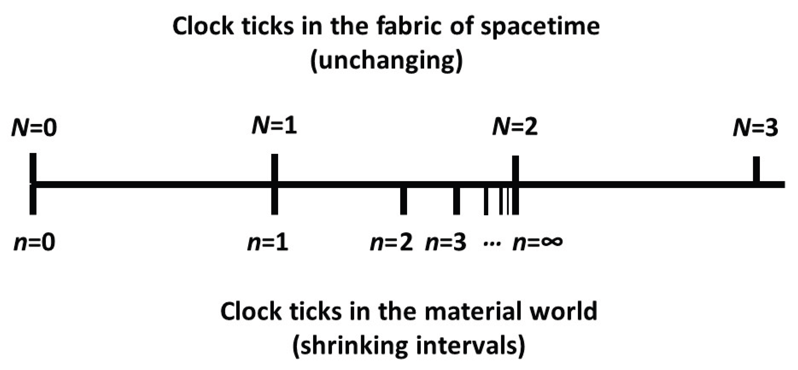
Figure 2.
Illustration of a physical system of two bodies of radius s, separation r, and initial separation velocity v0, in both the STM (lower case variable names) and STF (upper case) coordinate systems.
Figure 2.
Illustration of a physical system of two bodies of radius s, separation r, and initial separation velocity v0, in both the STM (lower case variable names) and STF (upper case) coordinate systems.
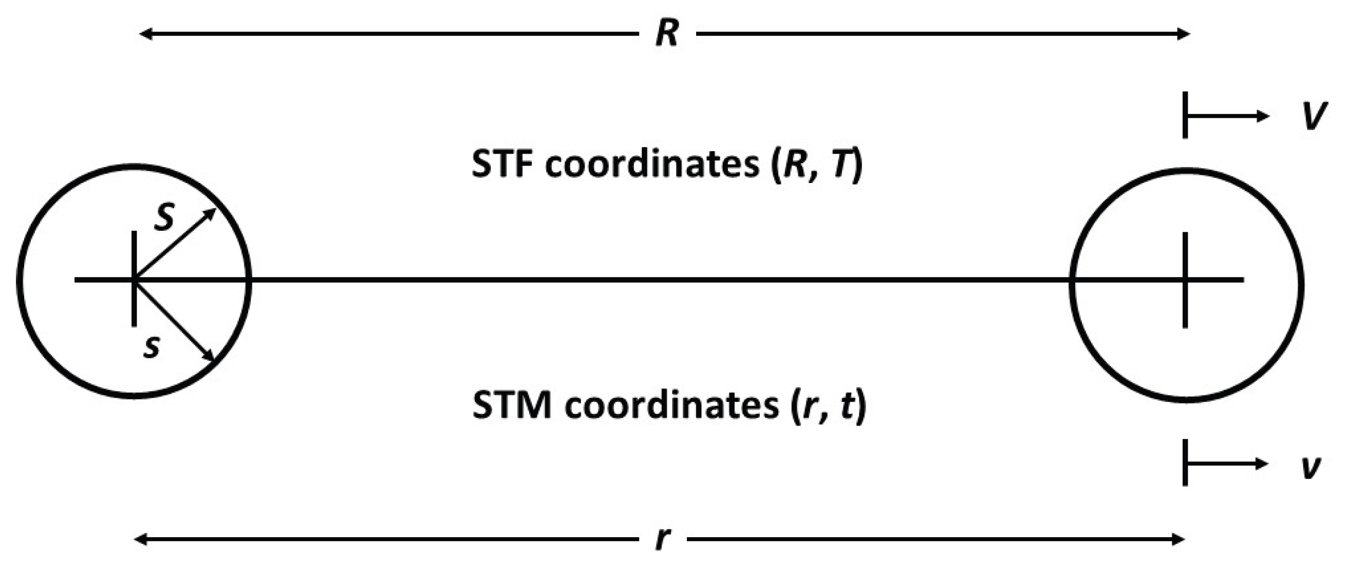
Figure 3.
Comparison of SIC model predictions (thin lines with symbols) to the DESI fits (thick lines without symbols) for the apparent dark energy density. The DESI fit using scale-independent angular data (BAO + CMB) (solid line without symbols) is notably different than the fits including supernovae data. The three SIC models have slopes within the envelope of the DESI fit slopes at a =1, the current time. The physically sensible dEdT SIC model most closely matches the DESI fits. The SIC models are all in STM units, whereas the DESI fits have lower values at earlier times due to the inclusion of CMB data, which is scale independent hence represents STF units and induces a 1/f2 reduction at lower a and higher f. This also explains why the DESI supernovae data are below the DESI BAO+CMB data at lower a. The right panel shows the same data with the SIC model parameters derived from a more limited range of least squares fit to the ΛCDM model (a= [0.8, 1.0] vs. [0.6, 1.0] ), showing the SIC results are only weakly dependent on the details of the DE model fit to ΛCDM. The apparent dark energy density from the DE and Lin-T SIC models would be a horizontal line of value one in these plots.
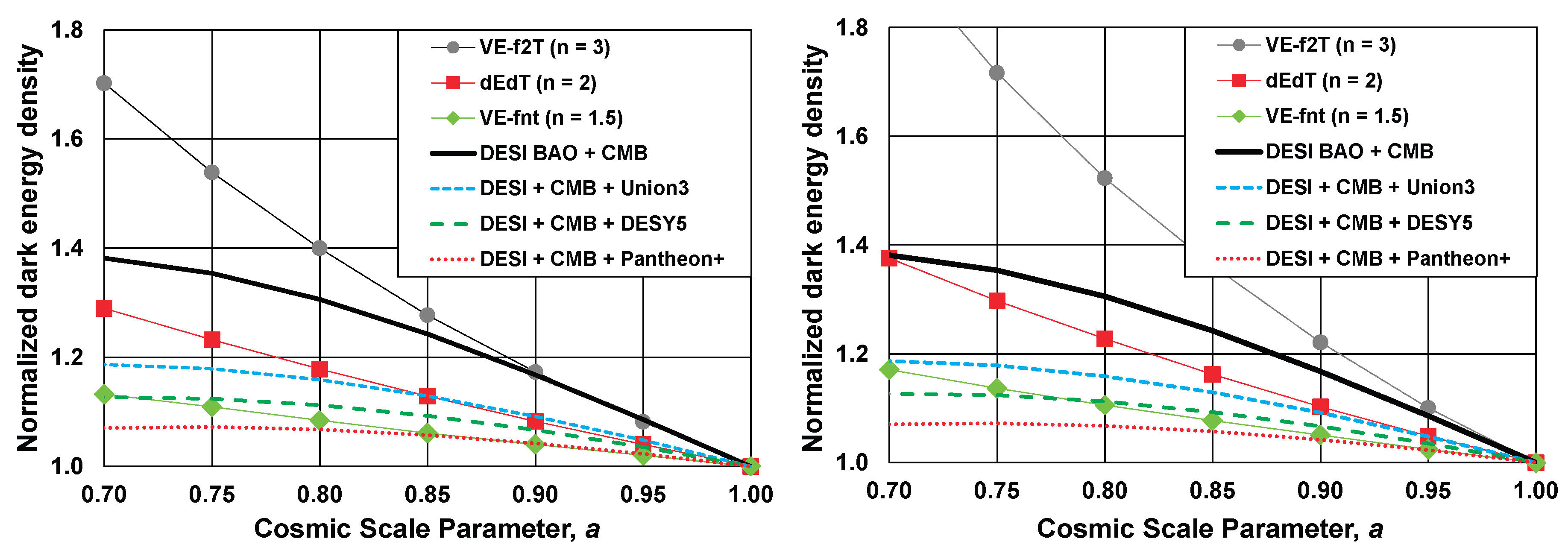
Figure 4.
Comparison of the scale factor, f, over time in STM units, with time starting at the Big Bang and f normalized to a current value of 1 for comparison. The value of n in the VE-fnt model is shown for each model to indicate how using n as a fit parameter with the VE-fnt model can discriminate between the different models. ΛCDM with a constant dark energy has constant f = 1 and corresponds to an extremely large value for n. VE-fnt with n=10 is shown to illustrate that the value of n should readily discriminate between the ΛCDM model and a SIC model. The DE/Lin-t and dEdT models imply the material world has contracted by 68% or 73%, respectively, of its scale at the Big Bang.
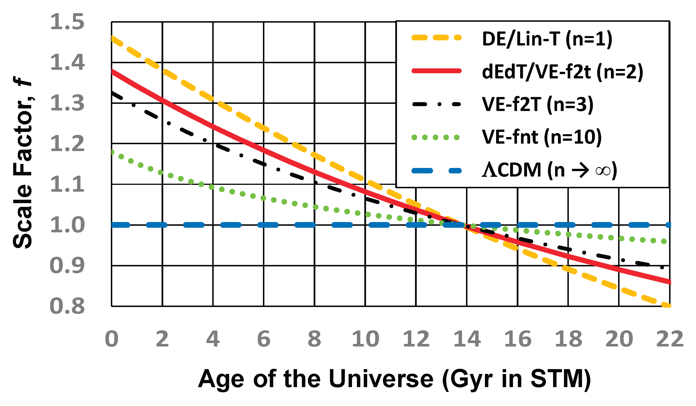

Table 1.
Considerations for the physical plausibility of models of the expansion of the universe: comparison of considerations with respect to the dark energy model, a generic scale-invariant model, and a scale-invariant vacuum energy model.
Table 1.
Considerations for the physical plausibility of models of the expansion of the universe: comparison of considerations with respect to the dark energy model, a generic scale-invariant model, and a scale-invariant vacuum energy model.
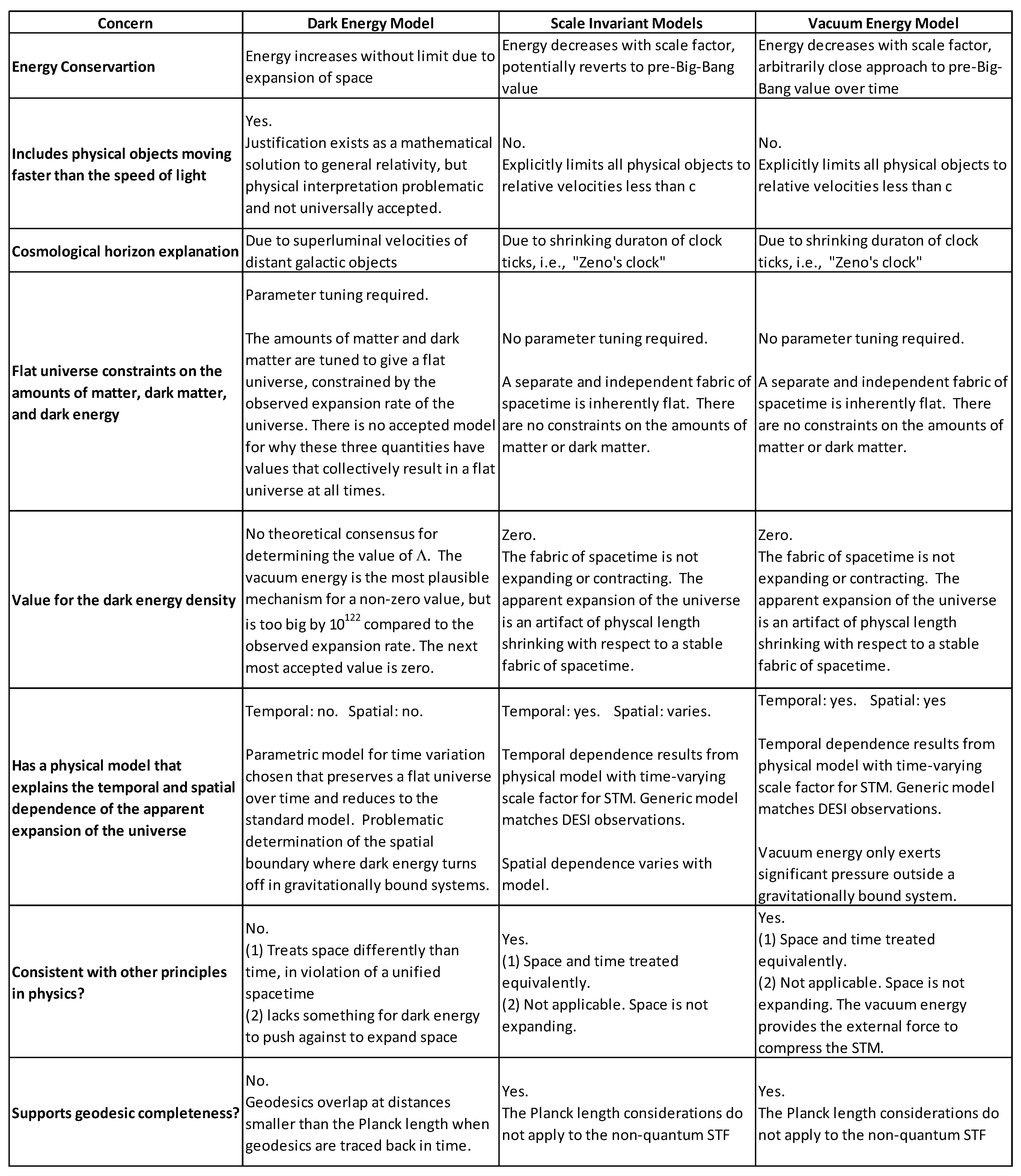
Disclaimer/Publisher’s Note: The statements, opinions and data contained in all publications are solely those of the individual author(s) and contributor(s) and not of MDPI and/or the editor(s). MDPI and/or the editor(s) disclaim responsibility for any injury to people or property resulting from any ideas, methods, instructions or products referred to in the content. |
© 2025 by the authors. Licensee MDPI, Basel, Switzerland. This article is an open access article distributed under the terms and conditions of the Creative Commons Attribution (CC BY) license (http://creativecommons.org/licenses/by/4.0/).
Copyright: This open access article is published under a Creative Commons CC BY 4.0 license, which permit the free download, distribution, and reuse, provided that the author and preprint are cited in any reuse.


