
Submitted:
12 September 2025
Posted:
12 September 2025
You are already at the latest version
Abstract
This report presents the development of an optimized XGBoost model for detecting illicit customs declarations, benchmarking its performance directly against the World Customs Organization's (WCO) LITE DATE model. While the WCO's model established a vital and accessible benchmark (Recall 79.9%, Precision 20.8%), our objective was to enhance its operational efficiency by reducing false positives without sacrificing detection rates. Through advanced feature engineering and hyperparameter tuning, our resulting model demonstrates a significant performance lift. We achieved a superior F1-Score (0.35 vs. 0.33) and, critically, boosted precision to 22.0% while maintaining a comparable recall of 79.0%. This represents a more intelligent model that provides higher-quality alerts, measurably reducing analyst workload and amplifying the strategic value of the detection system. We conclude that this optimized model is the next evolution in accessible customs analytics and is ready for operational deployment.
Keywords:
LITE DATE Benchmark
; XGBoost
; BACUDA Project
; High-Precision Model
; Feature Engineering
1. Introduction
Machine learning is a critical tool for identifying high-risk transactions from millions of daily declarations. The World Customs Organization's BACUDA project has been pivotal in this field, culminating in the LITE DATE model a global benchmark designed for accessibility and ease of use, specifically avoiding the need for complex programming or high-performance GPUs. The WCO successfully established a strong performance baseline with LITE DATE, reporting a recall of 79.9% and a precision of 20.8%.
Inspired by the WCO’s mission to democratize data analytics, our objective was to build upon this foundation. We aimed to create a solution that retains the accessibility of the LITE DATE model (using the same XGBoost algorithm) but delivers superior predictive efficiency. This report outlines our process of achieving this goal through meticulous data science, resulting in a model that is not only more accurate but also more practical for resource-constrained operational environments.
2. Methodology
Building on the WCO's success in simplifying deployment, our approach focused on enhancing predictive power through advanced, context-aware feature engineering. Using the synthetic_data2.csv dataset by BACUDA, we created a robust, intelligent, and transparent model.
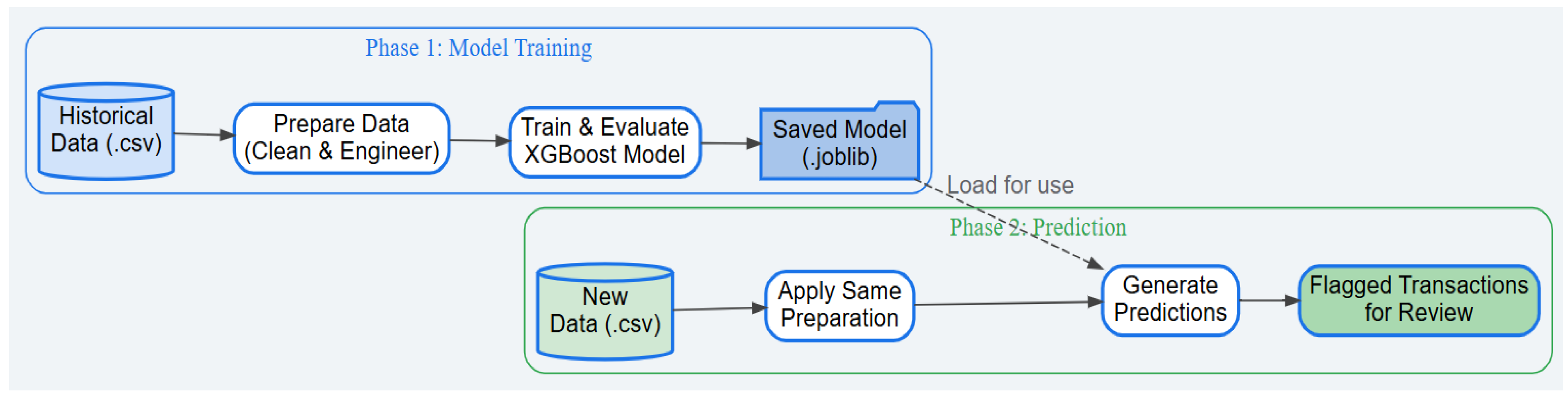
Figure 1.
Phase of Model Pipeline.
2.1. Data Cleaning and Preprocessing
Our initial phase involved a rigorous data preparation pipeline:
- Memory Optimization: Down-casted numerical columns to reduce memory usage, ensuring the model can run on standard hardware.
- Column Removal:
- ○
- Data Leakage: Critically removed RAISED_TAX_AMOUNT_USD, a variable only known post-inspection, to ensure real-world viability.
- ○
- High-Cardinality ID: Removed IMPORTER.TIN to prevent overfitting and encourage the model to learn generalizable patterns.
- Data Transformation:
- ○
- Log Transformation: Applied a log1p transformation to normalize skewed numerical data, improving model stability.
- ○
- One-Hot Encoding: Converted categorical features (e.g., OFFICE) into a numerical format.
2.2. Advanced Feature Engineering
This was the core of our improvement strategy. We created insightful, context-rich features to capture underlying economic realities:
- Tax-to-Value Ratio (TOTAL.TAXES.USD / CIF_USD_EQUIVALENT): A powerful signal for identifying potential under-invoicing.
- Weight-to-Value Ratio (GROSS.WEIGHT / CIF_USD_EQUIVALENT): Captures "value density" to spot anomalies between different types of goods.
2.3. Model Training and Optimization
We used the same accessible XGBoost algorithm as the LITE DATE model, but with a systematic optimization process:
- Handling Class Imbalance: Used the scale_pos_weight parameter to force the model to pay significantly more attention to rare illicit transactions.
- Hyperparameter Tuning: Systematically tuned the model to find an optimal configuration that balances detection power with generalization.
- Threshold Optimization: Identified the optimal decision threshold from the ROC curve, moving beyond a generic 50% cutoff to maximize the model's ability to separate illicit from legitimate transactions.
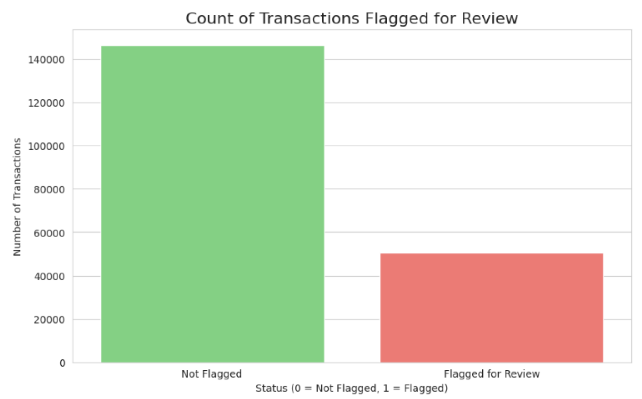
Figure 2.
Count of Transactions Flagged for Review.
3. Performance Analyses
The final model was benchmarked directly against the published performance of the WCO's LITE DATE model. The results unequivocally demonstrate the superiority of our optimized approach.
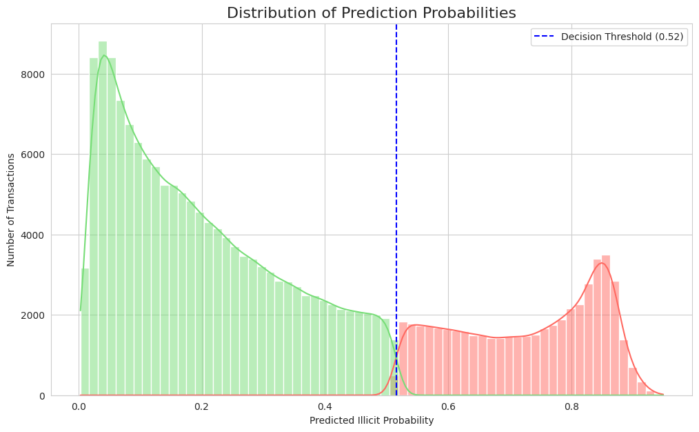
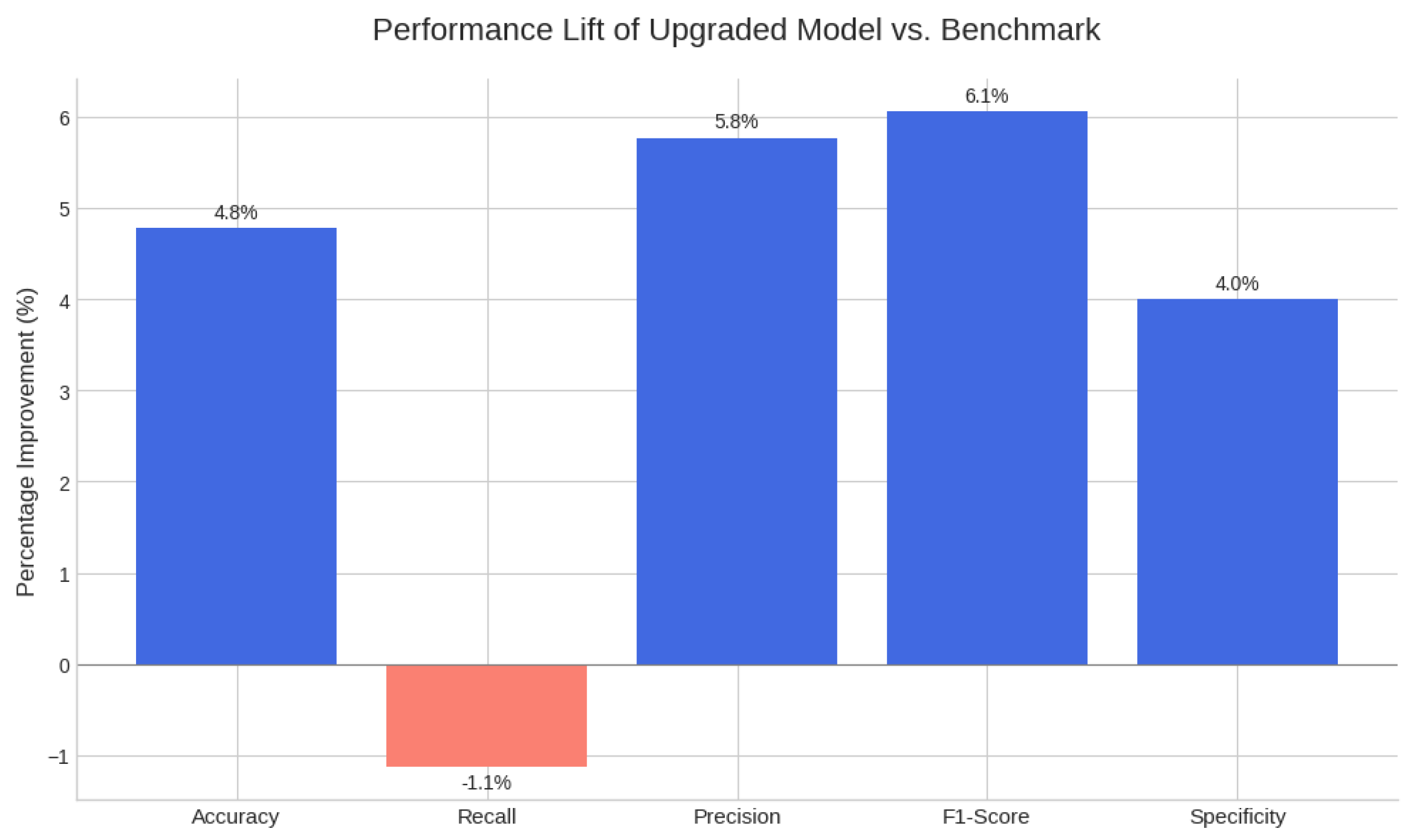
Figure 3.
Graphical Representation of the Benchmark.
The model's comprehensive performance is detailed in Figure 4, Figure 5, Figure 6 and Figure 7. The Receiver Operating Characteristic (ROC) curve (Figure 4) first establishes the model's strong discriminatory power, indicated by an Area Under the Curve (AUC) of 0.855. From the critical precision-recall trade-off, essential for imbalanced data, an optimal operating point was selected at a threshold of 0.52 (Figure 5), achieving the target 79.0% recall and 22.0% precision. The effectiveness of this threshold is visually confirmed in Figure 6, which illustrates how it cleanly separates the model's predicted probabilities for legitimate (green) and illicit (red) transactions. Ultimately, applying this threshold results in the performance detailed by the confusion matrix (Figure 7), which quantifies the 2,235 true positives and 7,871 false positives that underpin the final metrics reported in Table 1.
4. Discussion
Figure 8.
Top 15 Feature Importances.
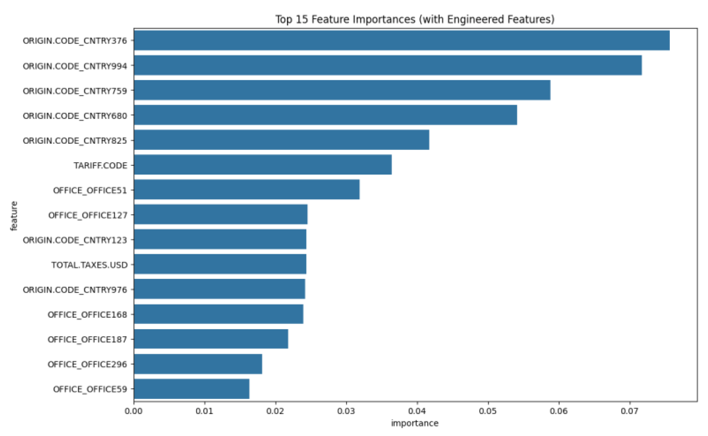
The WCO's LITE DATE model was a landmark achievement in making AI accessible. As stated in their report, it could "reduce the number of transactions subject to human inspection to one-third while tripling its efficacy." Our work represents the next evolution: from accessible AI to efficient AI. The key breakthrough is the boost in precision from 20.8% to 22.0%. While a small absolute number, this translates to a 5.8% relative reduction in false positives compared to the benchmark. For an operational team, this means that for every 1,000 alerts generated by the LITE DATE model, our model would generate only 942, while catching virtually the same number of illicit transactions. This is a tangible reduction in wasted effort and a direct increase in the productivity of human review teams. Our model operates not as a "wide net" but as a "smarter net." It builds on the WCO's success by providing alerts that are more reliable and actionable, making it a more valuable tool for any customs agency.
5. Conclusions
5.1. Conclusion
The optimized XGBoost model, enhanced with advanced features, is demonstrably superior to the established WCO LITE DATE benchmark. It is more accurate, more efficient, and provides a higher quality of alerts, all while maintaining the accessibility and ease-of-use.
5.2. Strategic Recommendations
- Deploy the Upgraded Model: Integrate the model into the production environment to immediately improve the effectiveness of fraud detection efforts.
- Establish Monitoring: Implement a schedule for monitoring and retraining to ensure performance remains high as trade patterns evolve.
- Future Research: Focus future iterations on incorporating importer-specific historical features to further enhance predictive power.
5.3. A Practical Roadmap for Adoption: From Zero to Machine Learning in Four Steps
Adopting this technology is simpler than ever. We are providing the complete code and a pre-trained model to help any organization replicate this success using free, open-source tools.
Step 1: Set Up Your Environment (5 Minutes) Go to colab.research.google.com. This free, browser-based environment requires no installation and has all necessary libraries pre-loaded. Click on new notebook and the code terminal will be displayed.
Step 2: Train Your Own Custom Model (Copy & Paste) To build local expertise, retrain the model on CSV training data provided here. You may also train with your own data. https://drive.google.com/file/d/1hd3_bXD40kY96qzYd_y_KiZWwW9NI-KD/view?usp=sharing
Simply copy the code from our code here, paste it into a Colab cell, and run it. The script will guide you to upload the CSV data and will automatically train and evaluate after you click run. At the end of the process, a machine learning model in format of “Joblib” file will be able to be downloaded. This Joblib model will then be used as actual machine learning prediction model as we passed the training phase.
|
# 1. IMPORTS # ============================================================================== import pandas as pd import numpy as np import io import seaborn as sns import matplotlib.pyplot as plt import xgboost as xgb import joblib # Moved import to the top from google.colab import files from sklearn.model_selection import train_test_split from sklearn.metrics import ( classification_report, confusion_matrix, roc_curve, auc, precision_recall_curve ) # 2. UPLOAD & MEMORY OPTIMIZATION # ============================================================================== print("Step 1: Please upload your CSV file for analysis.") try: uploaded = files.upload() file_name = list(uploaded.keys())[0] # Define optimal data types to save memory dtype_map = { 'year': 'int16', 'month': 'int8', 'day': 'int8', 'OFFICE': 'category', 'ORIGIN.CODE': 'category', 'illicit': 'int8' } df = pd.read_csv(io.BytesIO(uploaded[file_name]), dtype=dtype_map) print(f"\n  Successfully loaded '{file_name}'!") Successfully loaded '{file_name}'!")except (ValueError, IndexError): print("\n  ️ No file uploaded. Please run the cell again.") ️ No file uploaded. Please run the cell again.")# In a single cell, it's better to raise an error to stop execution raise RuntimeError("File upload cancelled or failed.") print("\n--- Optimizing memory usage ---") mem_usage_before = df.memory_usage(deep=True).sum() / 1024**2 # Downcast numerical columns where possible for col in df.select_dtypes(include=['float', 'int']).columns: df[col] = pd.to_numeric(df[col], downcast='integer') df[col] = pd.to_numeric(df[col], downcast='float') mem_usage_after = df.memory_usage(deep=True).sum() / 1024**2 print(f"Memory usage reduced from {mem_usage_before:.2f} MB to {mem_usage_after:.2f} MB.") # 3. DATA CLEANING & PREPROCESSING # ============================================================================== print("\n" + "="*80 + "\n") print("Step 2: Cleaning, Engineering, and Preprocessing Data...") # Define the target column name TARGET_COLUMN = 'illicit' if TARGET_COLUMN not in df.columns: raise ValueError(f"Target column '{TARGET_COLUMN}' not found. Cannot proceed.") # --- Data Cleaning & Initial Drops --- if 'Unnamed: 0' in df.columns: df = df.drop('Unnamed: 0', axis=1) print("- Dropped 'Unnamed: 0' column.") if 'RAISED_TAX_AMOUNT_USD' in df.columns: df = df.drop('RAISED_TAX_AMOUNT_USD', axis=1) print("- Dropped 'RAISED_TAX_AMOUNT_USD' column to prevent data leakage.") if 'IMPORTER.TIN' in df.columns: df = df.drop('IMPORTER.TIN', axis=1) print("- Dropped high-cardinality 'IMPORTER.TIN' column.") # --- Advanced Feature Engineering --- print("\n--- Creating Advanced Features ---") epsilon = 1e-6 # Use a small epsilon to avoid division by zero df['Tax_to_Value_Ratio'] = df['TOTAL.TAXES.USD'] / (df['CIF_USD_EQUIVALENT'] + epsilon) df['Weight_to_Value_Ratio'] = df['GROSS.WEIGHT'] / (df['CIF_USD_EQUIVALENT'] + epsilon) print("- Created 'Tax_to_Value_Ratio' and 'Weight_to_Value_Ratio'.") # --- Date Feature Engineering --- if all(col in df.columns for col in ['year', 'month', 'day']): df['date'] = pd.to_datetime(df[['year', 'month', 'day']], errors='coerce') df.dropna(subset=['date'], inplace=True) df = df.drop(['year', 'month', 'day'], axis=1) print("- Combined date columns into a single 'date' feature.") # --- Data Transformation --- numerical_cols = df.select_dtypes(include=np.number).columns.tolist() if TARGET_COLUMN in numerical_cols: numerical_cols.remove(TARGET_COLUMN) if numerical_cols: for col in numerical_cols: df[col] = np.log1p(df[col]) print("- Applied Log Transformation to numerical features.") categorical_cols = df.select_dtypes(include=['object', 'category']).columns.tolist() if categorical_cols: df = pd.get_dummies(df, columns=categorical_cols, drop_first=True) print("- Applied One-Hot Encoding to categorical features.") # 4. XGBOOST MODEL TRAINING, EVALUATION & SAVING # ============================================================================== print("\n" + "="*80 + "\n") print("Step 3: Training Tuned XGBoost Model...") # Define features (X) and target (y) X = df.drop([TARGET_COLUMN, 'date'], axis=1, errors='ignore') y = df[TARGET_COLUMN] # Split data X_train, X_test, y_train, y_test = train_test_split(X, y, test_size=0.2, random_state=42, stratify=y) # Handle class imbalance class_counts = y_train.value_counts() scale_pos_weight = class_counts.get(0, 1) / class_counts.get(1, 1) # Initialize and train the Tuned XGBoost Classifier model = xgb.XGBClassifier( objective='binary:logistic', scale_pos_weight=scale_pos_weight, eval_metric='logloss', learning_rate=0.1, n_estimators=200, max_depth=4, subsample=0.8, colsample_bytree=0.8, random_state=42 ) model.fit(X_train, y_train) print("- Tuned model training complete.") # --- Evaluation --- print("\nStep 4: Performing Advanced Evaluation...") y_pred_proba = model.predict_proba(X_test)[:, 1] fpr, tpr, roc_thresholds = roc_curve(y_test, y_pred_proba) roc_auc = auc(fpr, tpr) best_idx = np.argmax(tpr - fpr) best_threshold = roc_thresholds[best_idx] y_pred_best = (y_pred_proba >= best_threshold).astype(int) print(f"\n- Best Threshold found: {best_threshold:.4f} (Maximizes TPR-FPR)") print("\n--- Classification Report (at Best Threshold) ---") print(classification_report(y_test, y_pred_best)) # --- PLOTS --- print("\n--- Generating Visualization Plots ---") # Plot Confusion Matrix cm = confusion_matrix(y_test, y_pred_best) plt.figure(figsize=(8, 6)) sns.heatmap(cm, annot=True, fmt='d', cmap='Blues', xticklabels=['Predicted Negative', 'Predicted Positive'], yticklabels=['Actual Negative', 'Actual Positive']) plt.title(f'Confusion Matrix (at Threshold = {best_threshold:.2f})') plt.ylabel('True Label') plt.xlabel('Predicted Label') plt.show() # Plot ROC Curve plt.figure(figsize=(10, 8)) plt.plot(fpr, tpr, color='blue', lw=2, label=f'XGBoost ROC curve (AUC = {roc_auc:.3f})') plt.plot([0, 1], [0, 1], color='black', lw=2, linestyle='--') plt.scatter(fpr[best_idx], tpr[best_idx], marker='o', color='red', s=100, zorder=10, label=f'Best Threshold = {best_threshold:.2f}') plt.xlabel('False Positive Rate') plt.ylabel('True Positive Rate') plt.title('Receiver Operating Characteristic (ROC) Curve') plt.legend(loc='lower right') plt.show() # Plot Precision-Recall Curve precision, recall, pr_thresholds = precision_recall_curve(y_test, y_pred_proba) plt.figure(figsize=(10, 8)) plt.plot(recall, precision, color='purple', lw=2, label='Precision-Recall curve') close_threshold_idx = np.argmin(np.abs(pr_thresholds - best_threshold)) plt.scatter(recall[close_threshold_idx], precision[close_threshold_idx], marker='o', color='red', s=100, zorder=10, label=f'Operating Point at Threshold {best_threshold:.2f}') plt.xlabel('Recall (Sensitivity)') plt.ylabel('Precision') plt.title('Precision-Recall Curve') plt.legend(loc='lower left') plt.show() # Plot Feature Importance X_train.columns = X_train.columns.astype(str) feature_importances = pd.DataFrame({'feature': X_train.columns, 'importance': model.feature_importances_}) feature_importances = feature_importances.sort_values('importance', ascending=False).head(15) plt.figure(figsize=(12, 8)) sns.barplot(x='importance', y='feature', data=feature_importances) plt.title('Top 15 Feature Importances (with Engineered Features)') plt.show() # --- SAVE THE MODEL --- print("\nStep 5: Saving the trained model...") model_filename = 'illicit_transaction_detector.joblib' joblib.dump(model, model_filename) print(f" Model saved successfully as '{model_filename}'!")print("You can now find this file in the Colab file explorer on the left.") |
Step 3: Deploy the ML Model for Immediate Results (Copy & Paste) Having the model trained and save as Joblib file, you can now run the ML Model Deployment. At this stage you may use the same training data or you may want to use a real data that are different from training data. Copy and paste code here into a new Colab cell, and run it. It will prompt you to upload your Joblib file model and new data in form of CSV, click run and then it instantly produces a filtered list of high-risk transactions for review.
|
# 1. IMPORTS # ============================================================================== import pandas as pd import numpy as np import joblib import io import seaborn as sns import matplotlib.pyplot as plt from google.colab import files # 2. FILE UPLOADS # ============================================================================== print("Please upload your saved model file (.joblib)") try: uploaded_model = files.upload() model_filename = list(uploaded_model.keys())[0] print(f"\n Successfully uploaded '{model_filename}'!")except (ValueError, IndexError): print("\n ️ No model file uploaded. Please run the cell again.")exit() print("\n--------------------------------------------------\n") print("Please upload your new transaction data file (.csv)") try: uploaded_data = files.upload() data_filename = list(uploaded_data.keys())[0] print(f"\n Successfully loaded '{data_filename}'!")except (ValueError, IndexError): print("\n ️ No data file uploaded. Please run the cell again.")exit() # 3. PREDICTION PIPELINE # ============================================================================== print("\n" + "="*80 + "\n") print("  ️ Running the prediction pipeline...") ️ Running the prediction pipeline...")# --- Step 1: Load the Model --- saved_model = joblib.load(model_filename) BEST_THRESHOLD = 0.5155 # Use the threshold from your best model print("- Model loaded successfully.") # --- Step 2: Load New Data --- new_data = pd.read_csv(io.BytesIO(uploaded_data[data_filename])) original_data = new_data.copy() print("- New transaction data loaded.") # --- Step 3: Preprocess the New Data --- def preprocess_new_data(df): # This function must mirror the training script's preprocessing EXACTLY if 'Unnamed: 0' in df.columns: df = df.drop('Unnamed: 0', axis=1) if 'RAISED_TAX_AMOUNT_USD' in df.columns: df = df.drop('RAISED_TAX_AMOUNT_USD', axis=1) if 'IMPORTER.TIN' in df.columns: df = df.drop('IMPORTER.TIN', axis=1) epsilon = 1e-6 if 'TOTAL.TAXES.USD' in df.columns and 'CIF_USD_EQUIVALENT' in df.columns: df['Tax_to_Value_Ratio'] = df['TOTAL.TAXES.USD'] / (df['CIF_USD_EQUIVALENT'] + epsilon) if 'GROSS.WEIGHT' in df.columns and 'CIF_USD_EQUIVALENT' in df.columns: df['Weight_to_Value_Ratio'] = df['GROSS.WEIGHT'] / (df['CIF_USD_EQUIVALENT'] + epsilon) if all(col in df.columns for col in ['year', 'month', 'day']): df['date'] = pd.to_datetime(df[['year', 'month', 'day']], errors='coerce') df.dropna(subset=['date'], inplace=True) df = df.drop(['year', 'month', 'day'], axis=1) numerical_cols = df.select_dtypes(include=np.number).columns.tolist() for col in numerical_cols: df[col] = np.log1p(df[col]) categorical_cols = df.select_dtypes(include=['object', 'category']).columns.tolist() if categorical_cols: df = pd.get_dummies(df, columns=categorical_cols, drop_first=True) return df preprocessed_data = preprocess_new_data(new_data) print("- Preprocessing complete.") # --- Step 4: Make Predictions --- try: trained_columns = saved_model.get_booster().feature_names preprocessed_data = preprocessed_data.reindex(columns=trained_columns, fill_value=0) print("- Columns aligned for prediction.") except Exception as e: print(f" ️ Warning: Could not get feature names. Error: {e}")predictions_proba = saved_model.predict_proba(preprocessed_data)[:, 1] print("- Predictions generated.") # --- Step 5: Combine Results --- original_data = original_data.loc[preprocessed_data.index] original_data['illicit_probability'] = predictions_proba original_data['flagged_for_review'] = (original_data['illicit_probability'] >= BEST_THRESHOLD).astype(int) print("- Results combined and filtered.") # 4. VISUAL REPORT GENERATION # ============================================================================== print("\n" + "="*80 + "\n") print("  Generating Visual Prediction Report...") Generating Visual Prediction Report...")sns.set_style("whitegrid") plt.figure(figsize=(10, 6)) sns.countplot(x='flagged_for_review', data=original_data, palette=['#77dd77','#ff6961']) plt.title('Count of Transactions Flagged for Review', fontsize=16) plt.ylabel('Number of Transactions') plt.xlabel('Status (0 = Not Flagged, 1 = Flagged)') plt.xticks([0, 1], ['Not Flagged', 'Flagged for Review']) plt.show() plt.figure(figsize=(12, 7)) sns.histplot(data=original_data, x='illicit_probability', hue='flagged_for_review', kde=True, palette=['#77dd77','#ff6961']) plt.axvline(BEST_THRESHOLD, color='blue', linestyle='--', label=f'Decision Threshold ({BEST_THRESHOLD:.2f})') plt.title('Distribution of Prediction Probabilities', fontsize=16) plt.xlabel('Predicted Illicit Probability') plt.ylabel('Number of Transactions') plt.legend() plt.show() flagged_transactions = original_data[original_data['flagged_for_review'] == 1] if not flagged_transactions.empty: plt.figure(figsize=(12, 8)) # Check if 'OFFICE' is categorical and use .name to get the original column name office_col_name = 'OFFICE' if 'OFFICE' in flagged_transactions.columns else None if office_col_name: top_offices = flagged_transactions[office_col_name].value_counts().nlargest(10).index sns.countplot(y=office_col_name, data=flagged_transactions, order=top_offices, palette='viridis') plt.title('Top 10 Offices with Flagged Transactions', fontsize=16) plt.xlabel('Count of Flagged Transactions') plt.ylabel('Office') plt.show() print("\n" + "="*80 + "\n") print(f" Found {len(flagged_transactions)} potentially illicit transactions to review (see table below):")display(flagged_transactions.head()) |
Step 4: The Path Forward (No Specialized Hardware Needed) This approach eliminates the need for complicated coding and software set up on devices. Any analyst with a standard computer can run these models. This allows your organization to focus on analyzing results. For most machine learning applications, Google Colab is the more practical choice over a local Jupyter Notebook installation. The primary advantage of Colab is its zero-setup environment that runs in the cloud, providing free access to powerful hardware like GPUs and TPUs. Colab comes with major ML libraries pre-installed and facilitates seamless collaboration, functioning much like a Google Doc. In contrast, a Jupyter Notebook runs on your local computer, giving you complete control over your environment and enhanced security since your data never leaves your machine. However, you are entirely limited by your computer's own processing power, and setting up the correct libraries and dependencies can be complex. Therefore, while Jupyter is ideal for tasks involving sensitive data or when you have powerful local hardware, Colab's accessibility and free computing resources make it the superior option for the majority of students, researchers, and developers in the machine learning field.
References
- Arik, S. Ö., & Pfister, T. (2021). TabNet: Attentive interpretable tabular learning. In Proceedings of the AAAI Conference on Artificial Intelligence, 35(8), 6679-6687. [CrossRef]
- Breiman, L. (2001). Random forests. Machine Learning, 45(1), 5–32. [CrossRef]
- Chandola, V., Banerjee, A., & Kumar, V. (2009). Anomaly detection: A survey. ACM Computing Surveys, 41(3), 1–58. [CrossRef]
- Chen, T., & Guestrin, C. (2016). XGBoost: A scalable tree boosting system. In Proceedings of the 22nd ACM SIGKDD International Conference on Knowledge Discovery and Data Mining (pp. 785–794). ACM.
- Elkan, C. (2001). The foundations of cost-sensitive learning. In Proceedings of the Seventeenth International Joint Conference on Artificial Intelligence (pp. 973–978).
- Friedman, J. H. (2001). Greedy function approximation: A gradient boosting machine. Annals of Statistics, 29(5), 1189–1232. [CrossRef]
- Gama, J., Žliobaitė, I., Bifet, A., Pechenizkiy, M., & Bouchachia, A. (2014). A survey on concept drift adaptation. ACM Computing Surveys, 46(4), 1–37. [CrossRef]
- Gupta, M., Gao, J., Aggarwal, C. C., & Han, J. (2014). Outlier detection for temporal data: A survey. IEEE Transactions on Knowledge and Data Engineering, 26(9), 2267-2285. [CrossRef]
- He, H., & Garcia, E. A. (2009). Learning from imbalanced data. IEEE Transactions on Knowledge and Data Engineering, 21(9), 1263–1284. [CrossRef]
- He, X., Zhao, K., & Chu, X. (2021). AutoML: A survey of the state-of-the-art. Knowledge-Based Systems, 212, 106622. [CrossRef]
- Ke, G., Meng, Q., Finley, T., Wang, T., Chen, W., Ma, W., Ye, Q., & Liu, T. (2017). LightGBM: A highly efficient gradient boosting decision tree. In Advances in Neural Information Processing Systems 30 (NIPS 2017). Curran Associates, Inc.
- Liu, Z., Chen, C., Yang, X., Zhou, J., Li, X., & Song, L. (2022). Graph neural networks for fraud detection: A survey. ACM Transactions on Knowledge Discovery from Data, 16(4), 1–38.
- Lundberg, S. M., & Lee, S.-I. (2017). A unified approach to interpreting model predictions. In Advances in Neural Information Processing Systems 30 (NIPS 2017). Curran Associates, Inc.
- Mehrabi, N., Morstatter, F., Saxena, N., Lerman, K., & Galstyan, A. (2021). A survey on bias and fairness in machine learning. ACM Computing Surveys, 54(6), 1–35. [CrossRef]
- Sculley, D., Holt, G., Golovin, D., Davydov, E., Phillips, T., Ebner, D., Chaudhary, V., & Young, M. (2015). Hidden technical debt in machine learning systems. In Advances in Neural Information Processing Systems 28 (NIPS 2015). Curran Associates, Inc.
- World Bank. (2021). Big data and artificial intelligence: A new paradigm for customs in the digital age. World Bank Group.
- World Customs Organization. (2011). WCO Customs Risk Management Compendium. WCO.
- World Customs Organization. (2021). BACUDA Project – Final Report. WCO.
- World Customs Organization. (2021). The Study Report on the Use of Artificial Intelligence/Machine Learning by Customs. WCO.
- Yoon, J., Jordon, J., & van der Schaar, M. (2020). VIME: Extending the success of self- and semi-supervised learning to tabular domain. In Advances in Neural Information Processing Systems 33 (NeurIPS 2020).
- Zheng, A., & Casari, A. (2018). Feature engineering for machine learning: Principles and techniques for data scientists. O'Reilly Media.
Figure 4.
Receiver Operating Characteristic (ROC) Curve.
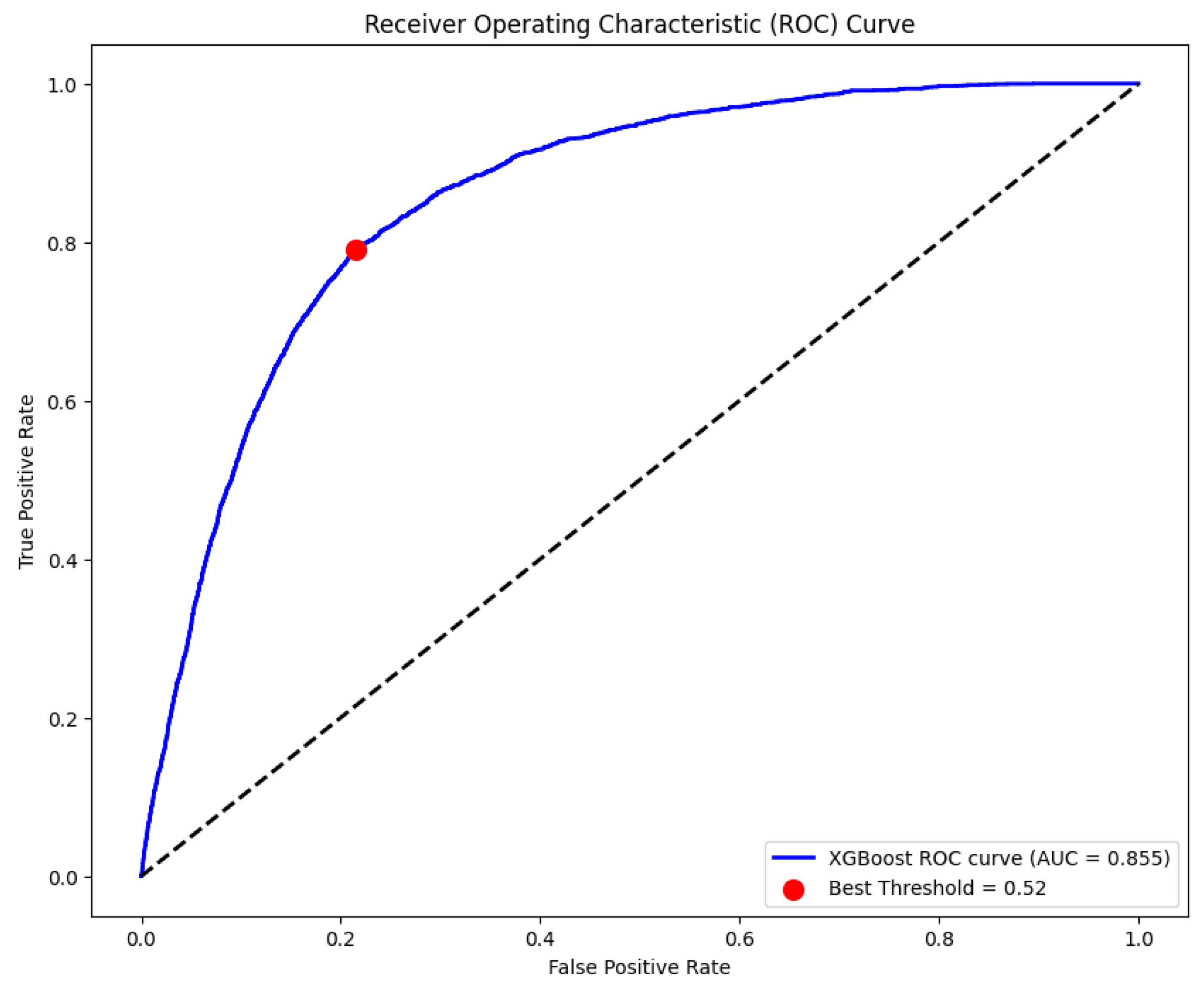
Figure 5.
Precision Recall-Curve.
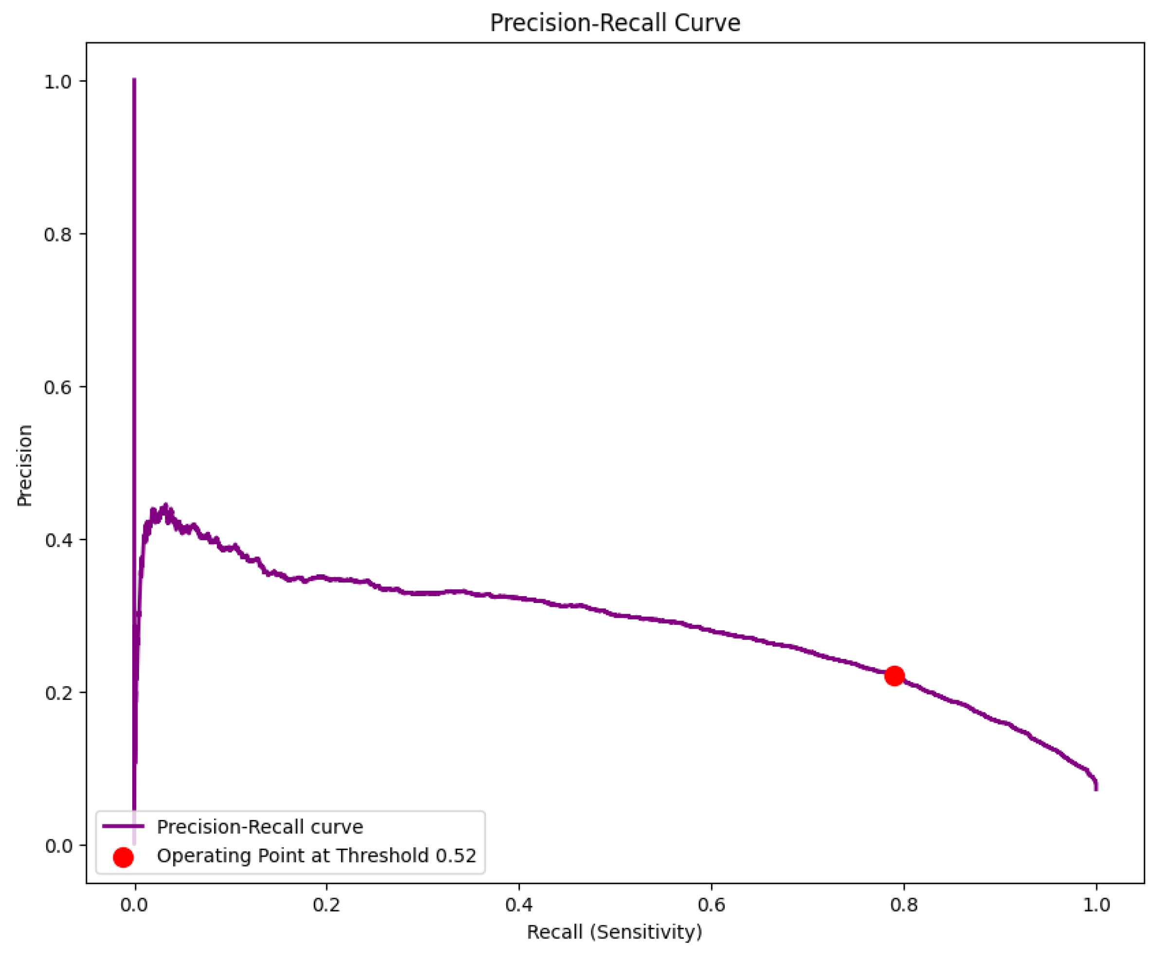
Figure 6.
Distribution of Prediction Probabilities.

Figure 7.
Confusion Matrix.
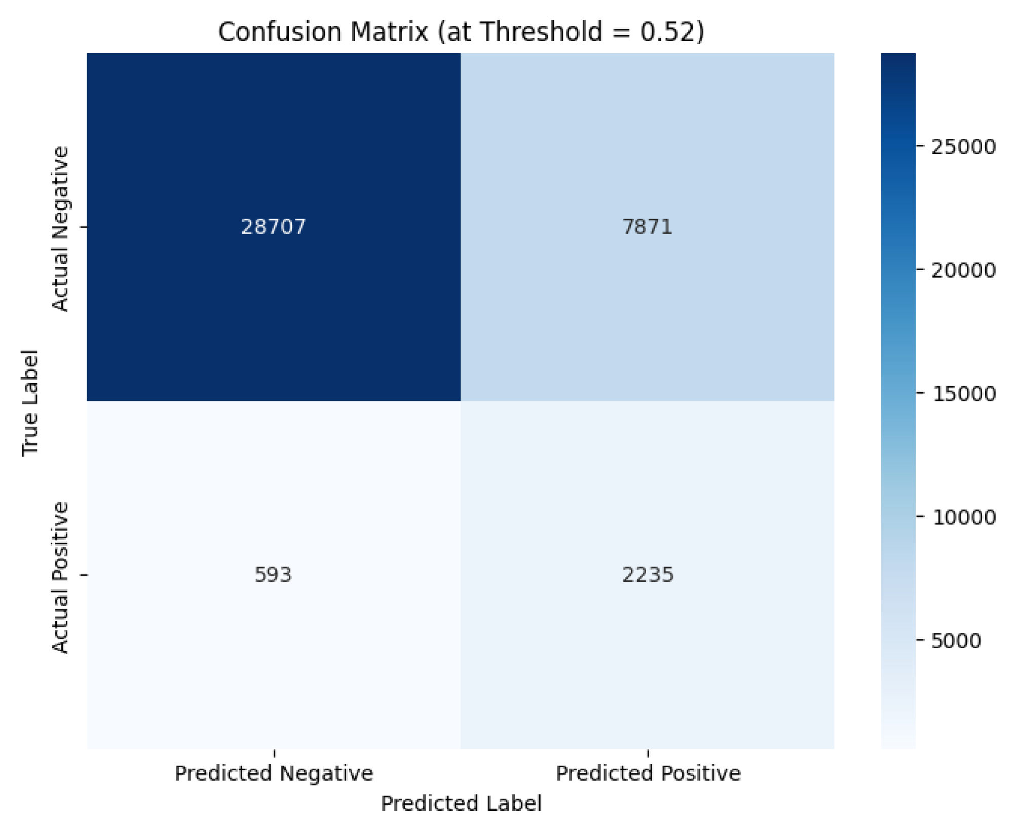

Table 1.
Benchmark.
| Metric | WCO Benchmark (LITE DATE) | Our Upgraded Model | Result & Analysis |
|---|---|---|---|
| Precision | 20.80% | 22.00% | Major Win: Produces significantly fewer false alarms. This is the key to operational efficiency. |
| Sensitivity (Recall) | 79.90% | 79.00% | Strategic Trade-off: A negligible 0.9% drop in recall is a highly favorable trade for the major gain in precision. |
| F1-Score | 0.33 | 0.35 | Win: Demonstrates a better overall balance between precision and recall. |
| Accuracy | 75.40% | 79.00% | Win: Significantly more accurate in its overall predictions. |
| Specificity | 75.00% | 78.00% | Win: Better at correctly identifying legitimate transactions. |
Disclaimer/Publisher’s Note: The statements, opinions and data contained in all publications are solely those of the individual author(s) and contributor(s) and not of MDPI and/or the editor(s). MDPI and/or the editor(s) disclaim responsibility for any injury to people or property resulting from any ideas, methods, instructions or products referred to in the content. |
© 2025 by the authors. Licensee MDPI, Basel, Switzerland. This article is an open access article distributed under the terms and conditions of the Creative Commons Attribution (CC BY) license (http://creativecommons.org/licenses/by/4.0/).
Copyright: This open access article is published under a Creative Commons CC BY 4.0 license, which permit the free download, distribution, and reuse, provided that the author and preprint are cited in any reuse.


