Submitted:
10 June 2025
Posted:
10 June 2025
You are already at the latest version
Abstract
Financial statement fraud remains a persistent challenge despite extensive audit work andadvances in AI-driven data processing. This study examines cases where engagements labeled as“low risk” nevertheless result in significant misstatements or irregularities. Using the public Big 4Financial Risk & Compliance dataset (2020–2025), an audit failure is defined when the ratio ofdetected fraud cases to high-risk cases falls below 0.5. Two tree-based classifiers—RandomForest and XGBoost—are trained on firm- and engagement-level features (total auditengagements, high-risk case count, revenue impact, employee workload, audit effectivenessscore, and AI usage). SHAP (SHapley Additive exPlanations) analysis ranks total revenue impact,employee workload, and audit effectiveness score as the strongest global risk drivers, whileindividual waterfall plots show how heavy workloads and lower effectiveness scores drive specificcases into the “failure” category—even when AI tools are deployed. Evaluated across fiveMD5-derived seeds, both models achieve over 95 % recall, demonstrating robust sensitivity indetecting audit failures. These results identify actionable audit levers—such as workloadmanagement and effectiveness improvements—to reduce undetected fraud, providing transparent,data-driven guidance for smarter audit practices and informing future regulatory standards.
Keywords:
fraud
; anomaly detection algorithms
; audit
1. Introduction
1.1. Background and Motivation
Anomaly detection aims to identify observations or events that deviate from expected patterns in data [1]. Also known as outlier detection—or variously termed discordant objects, exceptions, aberrations, peculiarities, or contaminants—these methods share the same fundamentals, with terminology chosen by application domain [1,2]. In financial systems, anomaly detection is chiefly applied to flag unusual transactions indicative of fraud. In this paper, we use “anomaly detection” throughout, resorting to “outlier detection” only when it better fits a particular methodological context.
Identifying anomalous patterns is crucial because deviations from normal behavior often signal important, actionable events—whether malicious activity, system faults, or emerging threats [1]. Anomalies can be induced for various reasons, in finical system, such anomalies might indicate credit-card identity theft or unauthorized transactions [3]. Traffic patterns that are anomalous in a computer network can indicate a malicious attempt to breach or compromise the system and lead to severe disruptions or even alert to a hacked computer that is sending sensitive data to an unauthorized destination [1,3]. Medical-image irregularities revealing malignant tissue in MRI scans [4,5]. Beyond these domains, sensor readings on spacecraft can pinpoint hardware failures, and precursor signals in geological data may foreshadow earthquakes [6,7]. In every case, anomaly detection relies on defining a “normal” model from which noteworthy outliers diverge [2].
In finance, fraud—including credit-card scams, insurance and healthcare fraud, money laundering, and securities manipulation—has ballooned into a multi-billion-dollar global problem, with U.S. losses alone exceeding $400 billion annually [8,9]. Such crimes not only impose direct costs (charge backs), administrative expenses, and eroded consumer trust on merchants [10,11]—but also fuel broader illicit activities like organized crime and drug trafficking [12]. These high stakes underscore the need for sophisticated anomaly-detection methods to catch evolving fraud tactics before they inflict further economic and social harm.
1.2. Research Objectives
Financial statement audits are essential for preserving market integrity by identifying and deterring corporate fraud. Yet, despite advances in methodology and the integration of analytics, major failures—exemplified by the Wirecard and Carillion collapses—show that even top-tier audit firms can miss material misstatements. This study examines why certain high-risk engagements nonetheless fail to detect fraud.
Using the publicly available “Big 4 Financial Risk & Compliance” dataset (2020–2025), which covers 100 audit engagements at PwC, Deloitte, EY, and KPMG, we define an audit failure as any cohort where fewer than half of the engagements flagged as high risk lead to confirmed fraud cases. This work addresses two central gaps:
Alignment between audit risk assessments and fraud outcomes While ML models can predict fraud with high accuracy, it is not well understood whether existing audit-risk proxies (e.g., high-risk case counts or audit effectiveness scores) truly correlate with detected fraud. We seek to quantify how often engagements flagged as low risk actually experience fraud and identify the factors most strongly associated with these audit failures.
Explainability of audit failure predictions. Even when a model flags certain low-risk engagements as high-risk, auditors need clear, interpretable guidance on which engagement-level features drove the misclassification. By employing SHAP (SHapley Additive exPlanations), we decompose tree-based model predictions to reveal both global feature-importance rankings and local, case-specific explanations.
To fill these gaps, we leverage the publicly available “Big 4 Financial Risk & Compliance” dataset, which spans 100 audit engagement records from 2020 to 2025 across the four largest global audit firms (PwC, Deloitte, EY, and KPMG).
After training tree-based models to predict fraud occurrences and apply SHAP (SHapley Additive exPlanations) to decompose predictions into both global feature-importance rankings and local, case-specific attributions. Our combined approach of threshold validation, robust prediction, and game-theoretic feature explanations quantifies when and why audit failures happen, and offers actionable recommendations—such as recalibrating workload distributions and refining risk metrics—to strengthen fraud detection in practice.
2. Literature Review
2.1. Overview of Fraud in Financial System
Financial fraud encompasses deliberate deception to secure unlawful financial gain. Although its exact origin is hard to pinpoint, records as early as 300 BC describe a bottomry scheme by the Greek merchant Hegestratos in Babylon: he plotted to scuttle his ship to claim insurance on vessel and cargo, but was ultimately foiled [13]. By 1911, fraud had permeated high-value art markets—Eduardo de Valfierno arranged the theft of the Mona Lisa from the Louvre to peddle expertly forged replicas to private collectors [14].
With the rise of digital commerce, identity theft emerged as a dominant fraud vector: criminals exploited stolen personal data (names, Social Security numbers, credit-card details) to open fraudulent accounts or execute unauthorized transactions. For example, in 2003 an Albertan used a stolen identity to purchase goods online, routed orders through North Dakota to obscure their destination, then repackaged and shipped them back to Edmonton [15].
As technology and trade methods advance, fraud unfortunately becomes increasingly sophisticated. While many people may associate it with phishing emails or spoofed mailings, the COVID-19 pandemic exposed vulnerabilities on an unprecedented scale: between 2020 and 2022, schemes against relief programs such as the Paycheck Protection Program (PPP) and state unemployment funds resulted in estimated losses of $100 billion to $400 billion [16]. Over 1,000 DOJ cases were filed to recover misappropriated funds, yet only a fraction has been reclaimed.
2.1.1. Credit Card Fraud
One of the most common frauds is credit card fraud. Especially the majority of people have already set credit card payment as their primary payment during the daily life over the past couple of decades. Heavily rely on credit card inveitable points to credit card fraud may involve with grave consequences, such as funding organized crime, narcotics trafficking, and even terrorist operations [8]. Report [17] indicates that global losses from fraudulent card transactions reached $28.65 billion in 2020, with the United States alone suffering $9.62 billion in losses—roughly one-third of that total. Several years ago, researchers have already warned that as credit-card usage continues to proliferate, a corresponding uptick in illicit activity is to be expected [8].
Generally, there are two principal types that people can follow to distinguish credit card fraud, ’application fraud’ and ’behavioral fraud’, which was often called "offline" and "online" fraud, respectively [18,19]. Application fraud occurs when criminals use stolen or fabricated personal details to open new credit-card accounts in someone else’s name. In contrast, behavioral fraud involves the illegal use of existing cards and breaks down into five main schemes [8,19].Mail-theft fraud:intercepting someone’s mail to steal physical cards or account information, which is then used to commit application fraud.Lost-or-stolen-card fraud:exploiting credit cards that have been mislaid or physically taken from their rightful owner. Counterfeit-card fraud:creating and using cloned cards after skimming magnetic-stripe data. Cardholder-not-present fraud:conducting unauthorized remote transactions (e.g., online or telephone purchases) without the physical card. Bankruptcy fraud:deliberately racking up charges with no intention to repay and then filing for personal bankruptcy to escape the debt—a form of fraud notoriously hard to detect [20].
The raw features used to describe credit card fraud are strikingly consistent in the surveyed literature. This consistency comes from the guideline of the International Financial Reporting Standards (IFRS) Foundation guidelines, which credit-card issuers and financial institutions must follow IFRS Foundation [21]. The most common raw features appearing in these datasets are summarized below Table 1 [22].
2.1.2. Insurance Fraud
Insurance fraud is another common type of financial fraud. Unlike credit card fraud, it involves deliberate deception at any stage of the claims process, whether perpetrated by policyholders, healthcare providers, insurance employees, agents, or brokers [23]. While it most frequently targets the health and auto–insurance sectors, incidents also occur in crop and homeowners’ policies, albeit with less scholarly coverage [24]. In the United States, such fraud costs exceed $80 billion each year, expenses that are ultimately passed on to consumers through higher premiums [25].
Among various forms of insurance fraud, detection efforts have most intensely focused on automobile policies [23]. A 2012 KPMG study commissioned by the Insurance Bureau of Canada estimated that Ontario insurers lost over $1.6 billion to fraudulent auto-insurance claims that year [25]. Moreover, research indicates that 21 % to 36 % of auto-insurance claims show signs of fraud, yet fewer than 3 % of those flagged cases ever lead to prosecution [26,27].
Other than automobile insurance fraud, another main category is healthcare insurance fraud. Today, healthcare has evolved into a complex domain where healthcare has become a significant concern that is tangled with political, social, and economic issues. A growing problem has been the abuse and exploitation of healthcare insurance systems by fraudsters for benefits they or someone else may not be entitled to. Healthcare providers have also been found to exploit the system for financial gain through practices inconsistent with sound fiscal, business, or medical practices. This results in unnecessary costs or reimbursements for services not medically necessary or that fail to adhere to professionally recognized standards for healthcare [28]. It has been reported by the National Health Care Anti-Fraud Association (NHCAA) that the total losses due to fraudulent healthcare insurance claims in the United States are estimated, conservatively, to have exceeded $100 billion in 2018, approximately 3% of the total expenditure on healthcare that year which was $3.6 trillion [25]. However, some government and law enforcement agencies estimate the losses to reach as high as 360 $ billion. [29] was one of the first to describe two distinct healthcare-insurance fraud profiles: in a “hit-and-run” scheme, fraudsters file a large batch of bogus claims and disappear once they receive payment, whereas those who “steal a little, all the time” submit many smaller fraudulent claims over an extended period, keeping each under the radar to avoid detection.
2.1.3. Other types Fraud
Other than the two mentioned types of fraud, there are still other types of fraud, such as money laundering or securities fraud. Money laundering is the process by which criminals or terrorist organizations “clean” illicit proceeds—often derived from drug trafficking, human smuggling, or the financing of extremist activities—by disguising their origins and integrating them into the legitimate financial system. This global scourge not only inflicts severe economic damage but also undermines the stability and integrity of financial institutions, fostering corruption in both the public and private sectors and deterring foreign investment in affected countries [12].
Beyond laundering, the financial domain hosts a diverse array of frauds. Securities and commodities fraud encompasses pyramid and Ponzi schemes, prime-bank and high-yield investment scams, market manipulation, and more, all enabled by increasingly integrated global capital markets [25].
2.2. Traditional Fraud-Detection Techniques
Rule-Based Systems:Traditional fraud detection often relies on rule-based systems, which use predefined rules and conditions to identify potentially fraudulent transactions or activities. For instance, a rule might be set to flag any transaction exceeding a specific amount, or one that originates from a location outside of a customer’s typical spending patterns. These systems are relatively straightforward to implement and can be effective at detecting known and basic fraud patterns. However, they often struggle to adapt to new or evolving fraud tactics and can generate a high number of false positives when legitimate activities deviate from the established rules. However, rule-based system was first developed by artificial intelligence researcher [30].
Manual Reviews:Before the widespread adoption of automated systems, manual reviews by human analysts were a primary method of detecting fraud. Analysts would meticulously examine transactions and accounts, particularly high-value ones or those with unusual behaviors, to identify potential fraud. While human intuition and judgment can be valuable in detecting subtle and complex fraud schemes, manual reviews are labor-intensive, time-consuming, and prone to human error. They also pose scalability issues as transaction volumes increase.
Statistical Methods:Statistical methods have also been used for years to identify anomalies or outliers in transactional data. Techniques like regression analysis, clustering, and various statistical tests examine historical data to establish benchmarks and identify deviations from normal patterns. For example, anomaly detection focuses on identifying unusual transactions or behaviors that deviate significantly from expected patterns, assuming that fraudulent activities often stand out from the norm. Statistical methods are generally more accurate than simple rule-based systems in identifying nuances in data but may require significant computational resources and expertise for set up and analysis.
2.3. Common Algorithms
Financial-fraud detection typically blends several algorithmic approaches to balance accuracy, adaptability, and scalability. Supervised classifiers—such as logistic regression, decision tree, and their en sembles (random forests, gradient-boosting machines), support vector machines, and deep neural networks—learn to distinguish fraudulent from legitimate transactions using labeled examples. Complementing these are unsupervised anomaly-detection methods, including Isolation Forests, one-class SVMs, density-based techniques like Local Outlier Factor, and reconstruction-based models such as autoencoders or PCA, which flag unexpected patterns without requiring extensive fraud labels. Hybrid and ensemble strategies often layer expert rules or supervised filters with anomaly scores, combining multiple detectors to reduce false positives and capture diverse fraud schemes. More recently, graph-based algorithms—such as graph neural networks that model transaction networks—and advanced deep-learning architectures (GAN-based detectors and sequence models like LSTM autoencoders or transformers) have been adopted to uncover complex relational and temporal anomalies. This multi-pronged algorithmic toolkit enables financial institutions to respond to evolving fraud tactics while managing challenges like class imbalance, interpretability, and real-time processing.
3. Methodology
In this chapter, we present the methodological approach used to develop and evaluate our anomaly-based fraud detection system. First, we describe the end-to-end framework that transforms raw transaction data into a model-ready format. Next, we detail the specific anomaly detection algorithms such as Isolation Forest, One-Class SVM, and Autoencoders—chosen for their complementary strengths in identifying outliers. Finally, we outline our hyperparameter tuning and model selection process, which leverages cross-validation and performance metrics such as precision, recall, and false-alarm rate to optimize each model for real-world deployment. Together, these steps ensure a rigorous, reproducible evaluation of our proposed fraud detection pipeline.
3.1. Methodological Framework
In this study, we adopt a three-stage framework to ensure rigor and reproducibility in our anomaly-based fraud detection pipeline. First, we establish a data pipeline that fetches raw transaction records, applies cleaning and feature-engineering routines, and produces a normalized dataset suitable for modeling. Next, our experimental design specifies how data are partitioned and which baselines are used for comparison. Finally, we define a suite of evaluation metrics to assess detection performance both statistically and operationally.
3.1.1. Data Preparation Pipeline
Data preparation begins with the consolidation of raw inputs—such as transaction logs, user metadata, and system events—into a unified dataset. Preprocessing routines then address missing or invalid entries through imputation or record removal and enforce consistency checks (e.g., valid timestamps, nonnegative values). Feature construction follows, deriving statistical aggregates (rolling-window counts, moving averages), temporal deltas (time since last event), and categorical encodings (one-hot or embedding representations) that capture behavioral and contextual nuances. A final normalization or scaling step (e.g., z-score standardization or min–max rescaling) ensures feature distributions are compatible with assumptions made by subsequent detection algorithms.
3.1.2. Experimental Design
Experimental design defines how the prepared data are partitioned and which benchmarks are employed. Chronological splitting simulates real-time deployment by reserving the most recent observations for validation and testing, while k-fold cross-validation quantifies performance variability across different data subsets. Baseline detectors—ranging from simple rule-based thresholds to supervised classifiers trained on labeled examples—provide reference points against which anomaly-based methods are compared. Hybrid architectures may be specified by layering business-rule filters upstream of anomaly scorers, reflecting typical production workflows.
3.1.3. Evaluation Metrics and Operational Criteria
Evaluation employs both statistical metrics and operational criteria. Precision, recall, and F1-score at selected detection thresholds offer insight into true-positive versus false-positive trade-offs, while the area under the precision–recall curve (AUPRC) accounts for severe class imbalance. Specificity or false-alarm rate per thousand records further characterizes practical detection costs. Operational metrics—including average inference latency, memory and CPU usage during scoring, and ease of model retraining—assess a method’s suitability for real-time monitoring. Together, these measures ensure that selected algorithms strike an appropriate balance between detection effectiveness and deployment feasibility.
3.2. Anomaly Detection Algorithms
Among the many emerging methods, this section focuses on three algorithms that have proven effective in financial-fraud detection. Isolation Forest isolates anomalies through random feature-space partitioning with minimal preprocessing, enabling it to scale across massive transaction datasets. One-Class SVM learns a tight boundary around “normal” data in high-dimensional space and flags any instances that fall outside it. Autoencoder-based detection trains a neural network to reconstruct typical patterns and uses elevated reconstruction error to identify complex, non-linear deviations. Each algorithm is examined with respect to its underlying principles, critical hyper parameters, computational demands, and suitability for real-world fraud-monitoring systems.
3.2.1. Tree-Based Method
As an example of tree-based methods, we employ the Isolation Forest (IF) algorithm (IF) as an example to illustrate. The Isolation Forest (IF) algorithm employs two key properties of anomalies: they are rare and exhibit attribute values distinct from the bulk of the data [31]. IF constructs an ensemble of isolation trees (iTrees) by recursively partitioning the dataset: at each internal node, a random feature and split value are chosen, and the process continues until either a predefined tree height is reached or nodes contain only one instance. When a data point is separated with only a few splits—appearing near the root of an iTree—it is likely an anomaly. Normal observations, by contrast, require many splits and end up deeper in the tree. The number of splits, or path length from the root to the leaf node, becomes the anomaly score: the shorter the path, the more likely the point is anomalous. Figure 1 is an example showing the tree structure consists of a root node, external node, internal node, and edge [32].
3.2.2. Boundary-Based Method
Support Vector Machines (SVMs) are the prototypical boundary-based classifiers, producing a hyperplane (or kernelized surface) to separate classes. SVM was first introduced by Vapnik in 1995 to solve the classification and regression problems. The basic idea of SVM is to derive an optimal hyperplane that maximizes the margin between two classes [33]. A key advantage of SVMs is their ability to discover nonlinear decision boundaries by mapping the original inputs through a nonlinear function into a higher-dimensional feature space. In this transformed space F, points that weren’t separable by a straight line in the input space become linearly separable by a hyperplane. When that hyperplane is mapped back into the original input space I, it takes the form of a nonlinear curve.
Mathematically, given n training data samples:
SVM is formulated by the following optimization problem:
subject to
where the kernel function maps training points from input space into a higher dimensional feature space. The regularization parameter C controls the trade-off between achieving a low error in the training data and minimizing the weight norm.
3.2.3. Reconstruction-Based Method
In reconstruction-based anomaly detection, models are trained to accurately recreate “normal” data and then flag any inputs whose reconstruction error exceeds a threshold. Autoencoders—a common neural-network implementation of this idea—learn compact feature representations of the input and use them to reconstruct the original data, often serving as a form of nonlinear dimensionality reduction. In their simplest form, autoencoders are feedforward, non-recurrent networks similar to multilayer perceptrons [34]. As shown in Figure 2, an autoencoder consists of two parts—an encoder and a decoder—each built from an input layer, one or more hidden layers, and an output layer. Crucially, unlike conventional multilayer perceptrons, an auto encoder’s output layer matches the size of its input layer, since its goal is to reproduce the inputs rather than predict external targets.
In autoencoder, the network structure has connections between layers, but has no connection inside each layer, is input sample, is output feature.
The training of autoencoder neural network is to optimize reconstruction error using the given samples. The cost function of autoencoder neural network defined in the project is below
where m represents number of input samples
3.3. Hyperparameter Tuning and Model Selection
Hyperparameter tuning adapts each anomaly detector to the specific characteristics of financial-fraud data—such as severe class imbalance and shifting behavior patterns. For tree-based methods like Isolation Forest, tuning involves adjusting the number of trees, subsample size, and assumed contamination rate; for SVM, it requires selecting the kernel type and parameter; and for autoencoders, it means choosing network depth, learning rate, and reconstruction-error thresholds. Common search strategies include grid search for exhaustive coverage, random search for faster approximations, and Bayesian optimization for more efficient exploration of promising regions.
Determining the anomaly-score threshold is a critical step shared by all unsupervised and semi-supervised detectors. Thresholds can be set by selecting a fixed percentile of the score distribution (e.g., top 1%), by analyzing results to balance detection and false-alarm rates, or by applying cost-sensitive criteria that weigh the financial impact of missed fraud versus false positives. Aligning these cutoffs with operational tolerances—such as an acceptable false-alarm rate per thousand transactions—ensures the model’s behavior matches real-world risk and resource constraints.
Model selection compares tuned variants across algorithm families using unified metrics (precision, recall, F1-score) alongside practical considerations like inference latency, memory footprint, and interpretability. A Pareto-optimal front highlights solutions that offer the best trade-offs, while hybrid or ensemble pipelines—combining expert rules with multiple anomaly scorers—can leverage complementary strengths when no single model dominates. This multi-criteria selection process ensures the chosen detector balances statistical performance with the operational demands of fraud-monitoring systems.
4. Experimental set up and Results
In order to provide a clear point of experimental set up and results, this section introduces our baseline model within the three-stage methodological framework outlined previously. This foundational classifier is a Random Forest trained on the normalized transaction dataset—where missing values are imputed and rolling-window features are generated—using default hyperparameters chosen to balance interpretability and computational efficiency. Training follows a stratified train-test split, and all randomness is controlled via fixed seeds to guarantee reproducibility. Evaluation of this baseline employs both statistical metrics and operational measures to capture performance from multiple perspectives. The implementation leverages Python’s scikit-learn library on a standard workstation (Intel i7 CPU, 16 GB RAM), and the following subsections provide detailed descriptions of the model architecture, training procedure, and software environment.
4.1. Baseline model
4.1.1. Model Specification
In our code, we have employed random forest (RF) and XGBoost. The RF is an ensemble learning model for classification, regression, and other tasks [35]. The RF model utilizes decision trees to classify data and employs the bagging (i.e., bootstrap aggregating) approach to avoid the overfitting problem caused by complex decision trees. The Random Forest baseline is implemented using scikit-learn’s “RandomForestClassifier” with 200 trees (), a maximum tree depth of 10 (), and at least two samples required to form a leaf node (). These settings strike a balance between capturing complex feature interactions and preventing overfitting on our 100-record dataset. By constraining depth and leaf size, we ensure individual trees remain interpretable and generalize well, while the ensemble of 200 trees provides robustness against variance. The parameter fixes all sources of randomness—both in bootstrap sampling and feature selection—thereby guaranteeing reproducible results across multiple runs.
For XGBoost, our gradient-boosted baseline leverages XGBClassifier with 50 boosting rounds (), a maximum tree depth of 6 (), and a learning rate of 0.1 (), optimizing log-loss () to directly improve probabilistic calibration. We disable the legacy label encoder () to maintain compatibility with recent library versions. Limiting the number of estimators and tree depth helps mitigate overfitting risks inherent to small datasets, while the modest learning rate ensures stable convergence. As with the Random Forest, setting controls all internal randomness, allowing for exact reproducibility in our comparative analyses.
4.1.2. Hyperparameter Rationale
The chosen hyperparameters for our Random Forest baseline reflect a deliberate balance between model complexity and generalizability on a limited dataset. By setting , we ensure sufficient ensemble diversity to reduce variance without incurring excessive computational cost. The constraint prevents individual trees from growing overly complex and fitting to noise, while further regularizes leaf splitting to avoid overly specific partitions that could lead to high-variance predictions. Together, these settings maintain interpretability of the individual trees, keep training times reasonable on a modest workstation, and mitigate overfitting risks inherent to small-sample learning.
For the XGBoost classifier, we similarly calibrate hyperparameters to support stable convergence and guard against overfitting. Limiting the number of boosting rounds to and capping tree depth at restricts the model’s capacity to memorize idiosyncratic patterns, which is crucial when only 100 records are available. A moderate controls the contribution of each tree update, smoothing the gradient descent process and allowing incremental improvements in log-loss () rather than abrupt fits. Disabling the legacy label encoder () streamlines workflows with newer library versions, and fixing ensures reproducibility of the gradient-boosting process. These settings collectively yield a robust, well-regularized baseline that can be reliably compared against more complex variants.
4.1.3. Training Procedure
We conduct model training using an 80/20 stratified split on our 100-record dataset to ensure the proportion of the Audit_Failure label remains consistent across training and test sets. This single split is repeated five times—once per seed from our MD5-derived list—to assess the stability of each classifier’s performance. In each iteration, we invoke: for function . In this function from X dataset and y dataset test_size=0.2, stratify=y, random_state=seed .
This looped procedure yields five independent train/test splits, allowing us to average metric outcomes and report both mean performance and variability.
Following data partitioning, each model is fit on ‘’/‘’ and then evaluated on ‘’/‘’. We capture classification reports via scikit-learn’s ‘classification_report’ (output_dict=True) and compute ROC-AUC scores using ‘roc_auc_score’. To explore threshold sensitivity, we also vary the decision cutoff around 0.5 on model-predicted probabilities and tally false negatives versus total fraud cases. This comprehensive procedure provides a robust baseline against which more advanced modeling strategies can be compared.
4.1.4. Feature Set
Our input matrix comprises eight continuous predictors—Year; Total_Audit_Engagements; High_Risk_Cases; Compliance_Violations; Total_Revenue_Impact; Employee_Workload; Audit_Effectiveness_Score; and Client_Satisfaction_Score—selected for their direct relevance to audit outcomes. We additionally include three categorical variables (Firm_Name, Industry_Affected, AI_Used_for_Auditing), each one-hot encoded to capture firm-specific patterns, industry sectors, and AI adoption status in auditing workflows. These features collectively reflect both operational volume and risk indicators critical to detecting potential failures.
Derived metrics such as Fraud_Detection_Ratio and the binary Audit_Failure label are used exclusively to define the target variable and are withheld from model training. By segregating feature engineering for prediction from target construction, we prevent information leakage and ensure our baselines learn only from predefined predictors. This clear delineation of inputs versus derived signals maintains the integrity of our experimental design.
4.1.5. Reproducibility Controls
To guarantee full reproducibility, we generate five distinct integer seeds by MD5-hashing a base identifier (student ID = 310879), resulting in (1720342983, 1434932713, 1901833849, 158634399, 576778549). In each training loop, we set both Python’s ‘random.seed(seed)’ and NumPy’s ‘np.random.seed(seed)’, and pass ‘random_state=seed’ into all scikit-learn and XGBoost routines. These steps fix the randomness inherent in data splitting, bootstrap aggregation, and tree construction.
All code is version-controlled and executed under a consistent software stack—Python 3.11 (Anaconda), scikit-learn v1.x, XGBoost v1.x (CPU only), and SHAP v0.41.x—on the same Intel-based MacBook environment. By rigidly controlling both seeds and software versions, we ensure that any researcher can replicate our baseline results exactly, facilitating transparent comparisons in follow-on experiments.
4.1.6. Implementation Environment
Experiments are executed in Python 3.11 within the Anaconda distribution on an Intel-based MacBook (macOS) without GPU acceleration. Model fitting, data splitting, and metric computations utilize scikit-learn v1.x, while gradient boosting is handled by the CPU-only build of XGBoost v1.x. Post-hoc explainability analyses employ SHAP v0.41.x. Standardizing on these library versions and hardware ensures that results are not influenced by software or platform differences, enabling exact reproduction of the baseline performance.
4.1.7. Evaluation Metrics
Model performance is quantified using both statistical and operational measures. For each train–test split, accuracy, precision, recall, and -score are reported via scikit-learn’s classification report to capture overall correctness and class-specific detection capabilities. The area under the ROC curve (ROC-AUC) is computed on predicted probabilities to assess discriminative power independent of threshold choice. A sensitivity analysis is conducted by varying the decision threshold around 0.5 and recording changes in false-negative rates relative to total fraud cases. Finally, each metric’s mean and standard deviation across the five randomized splits are summarized to convey both central tendency and variability.
4.2. Data
The dataset we used in this project, it provides in-depth insights into financial risk assessment, compliance violations, and fraud detection trends in the Big 4 consulting firms – Ernst & Young (EY), PwC, Deloitte, and KPMG – from 2020 to 2025. It captures key metrics such as the number of audit engagements, high-risk cases, fraud cases detected, and compliance breaches. Additionally, it explores the impact of AI in auditing, employee workload, and client satisfaction scores.
4.2.1. Data Pipeline
The dataset consists of 100 audit engagement records from 2020 to 2025, each described by 12 fields encompassing operational, financial, and contextual information. In Table 2, the first five raw has been shown through code. And quick summary has been shown in table
Continuous predictors include Year, Total_Audit_Engagements (mean 2,784.5, SD 1,281.9, range 603∼4,946), High_Risk_Cases, Compliance_Violations, Fraud_Cases_Detected, Total_Revenue_Impact, Employee_Workload, Audit_Effectiveness_Score, and Client_Satisfaction_Score.

Table 3.
Quick summary of selected feature.
| Feature | Mean | Std Dev | Min | 25% | Median | 75% | Max |
| Total_Audit_Engagements | 2,784.5 | 1,281.9 | 603.0 | 1,768.3 | 2,650.0 | 4,008.8 | 4,946.0 |
| High_Risk_Cases | 277.7 | 135.7 | 51.0 | 162.5 | 293.0 | 395.5 | 500.0 |
| Compliance_Violations | 105.5 | 55.4 | 10.0 | 54.5 | 114.5 | 149.5 | 200.0 |
| Fraud_Cases_Detected | 52.7 | 28.3 | 5.0 | 27.0 | 54.0 | 74.5 | 100.0 |
| Total_Revenue_Impact (M USD) | 272.5 | 139.2 | 33.5 | 155.2 | 264.5 | 406.1 | 497.1 |
| Employee_Workload | 60.3 | 11.2 | 40.0 | 52.8 | 60.0 | 68.0 | 80.0 |
| Audit_Effectiveness_Score | 7.5 | 1.5 | 5.0 | 6.1 | 7.5 | 8.8 | 10.0 |
| Client_Satisfaction_Score | 7.3 | 1.4 | 5.0 | 6.1 | 7.4 | 8.5 | 10.0 |
Categorical predictors—Firm_Name (Deloitte 30%, PwC 25%, Ernst & Young 23%, KPMG 22%), Industry_Affected (Tech 29%, Retail 27%, Healthcare 24%, Finance 20%), and AI_Used_for_Auditing (Yes 45%, No 55%)—exhibit full coverage with no missing entries. Since all 100 records are complete, median- and mode-based imputation routines were defined but not invoked, and no records required discarding for excessive nulls. Several factors’ distribution from the raw data has been shown on Figure 3.
Feature construction begins with derivation of a Fraud_Detection_Ratio, computed as the number of cases detected divided by total engagements per audit. A binary Audit_Failure label is then created by thresholding this ratio at its sample median (≈0.0185), yielding a balanced split of 50 failures and 50 non-failures. Categorical fields are converted via one-hot encoding into indicator vectors for firm, industry, and AI-usage status. Although the annual resolution precludes meaningful rolling-window statistics, all static features are retained to capture both scale (e.g., revenue impact) and quality (e.g., effectiveness scores) dimensions.
4.2.2. Partitioning & Preparation
An 80/20 train–test partition is applied to the fully processed dataset, with stratification on the Audit_Failure label to preserve its 50:50 distribution in both subsets. This splitting procedure is repeated across five fixed seeds—derived via MD5 hashing of a base identifier—ensuring that each split is identical and that performance variability can be quantified. Random number in NumPy from python are initialized with the same seed before partitioning, guaranteeing that row order and class proportions remain constant across runs.
Prior to model fitting, continuous features are standardized by subtracting the mean and dividing by the standard deviation computed exclusively on the training data; the resulting scaling parameters are then applied to the test set to avoid information leakage. One-hot encoded categorical vectors maintain a consistent dimensionality across splits, and no further resampling or class-weight adjustments are necessary due to the initial stratification. This rigorous preparation ensures that subsequent model evaluations reflect genuine predictive capability rather than artifacts of data handling.
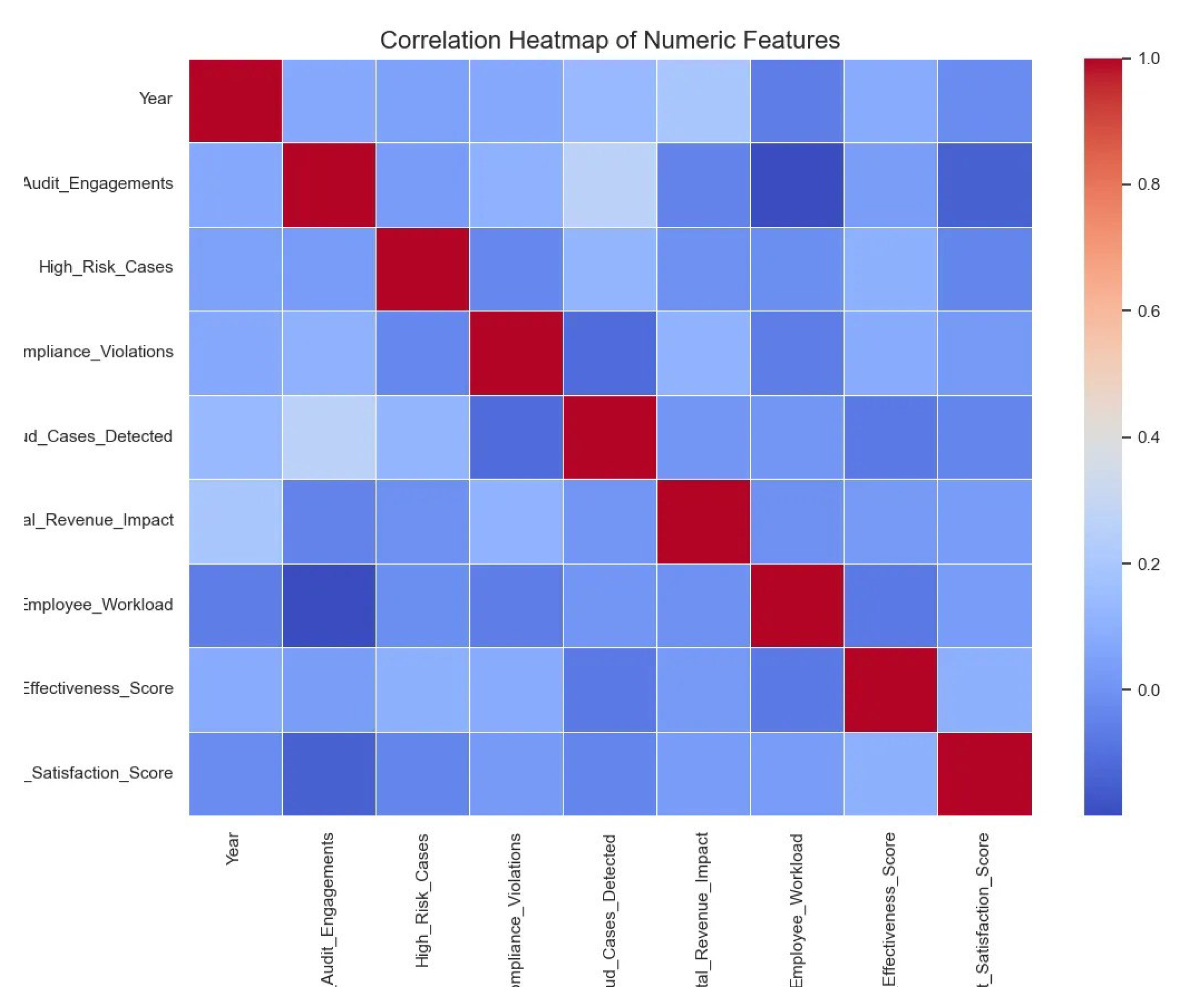
At the same time, the corelation heatmap was also generated. The correlation heatmap shows that nearly all numeric predictors exhibit only weak linear relationships (), indicating minimal multicollinearity. The strongest positive association () is between Total_Audit_Engagements and Fraud_Cases_Detected, suggesting that accounts audited more frequently tend to uncover more fraud. A moderate positive link () appears between Year and Total_Revenue_Impact, reflecting a temporal trend of increasing financial consequences over time. On the negative side, Total_Audit_Engagements and Employee_Workload correlate at about , implying that auditors handle lighter individual workloads when engagement counts are high. All other feature pairs, such as High_Risk_Cases vs. Compliance_Violations or Client_Satisfaction_Score vs. any other variable—hover near zero, justifying the use of each as a distinct input to the baseline models without major concern for redundancy.
Figure 4.
Corelation heatmap
4.3. Results
4.3.1. Evaluation Metrics
The primary performance indicators are derived from scikit-learn package classification_report, which yields accuracy, precision, recall, and for each class. Also from , which computes the area under the ROC curve based on model-predicted probabilities. These metrics provide both threshold-dependent (accuracy, precision, recall, ) and threshold-independent (ROC-AUC) assessments of each classifier’s ability to distinguish audit failures from non-failures.
To capture variability, each metric is calculated on the test set of each of the five stratified splits and then aggregated. Mean and standard deviation values for accuracy, precision, recall, , and ROC-AUC are reported, offering a concise view of central tendency and stability across different random seeds. The full report from RF and XGBoost are shown below in Table 4.
From the report ,both models default to predicting every case as “True,” achieving high recall on the majority class but completely missing the minority “False” cases. Macro-averaged metrics reflect this imbalance more starkly, while weighted averages mask it somewhat by giving more weight to the correctly classified majority class.
4.3.2. Baseline Performance
Baseline performance on the test split defined by seed 317325550 shows that both models correctly classified 17 of 20 instances, yielding an overall accuracy of 85% and perfect recall (100%) on the audit-failure class. In other words, every true failure was detected, but no true negatives were identified. The result has been shown in Table 5
This identical accuracy and recall across Random Forest and XGBoost underscores their shared bias toward capturing all failures—even at the expense of misclassifying non-failure cases. While this establishes a strong sensitivity baseline (zero missed failures), it also highlights the need to improve specificity in future model refinements.
An extended stability assessment using the CPU-optimized XGBoost (via tree_method=’hist’) over the five MD5-derived seeds yielded accuracy scores mean = 90 %, SD alongside recall values of . Full result has been shown below Table 6 . Such tight clustering around high performance confirms that the model’s ability to detect audit failures generalizes well beyond any single data split. While one seed produced perfect accuracy—suggesting certain partitions align especially well with the model’s inductive biases—even the lowest recall of 89.5% remains strong, underscoring robust sensitivity to the minority class across varied train–test configurations.
Figure 5 juxtaposes impurity-based importance scores from the Random Forest (left) and XGBoost (right) baselines. While both models agree that “Client_Satisfaction_Score” and “Total_Revenue_Impact” rank among the top predictors, XGBoost assigns greater weight to “Audit_Effectiveness_Score,” whereas Random Forest emphasizes “Employee_Workload.” The relative differences hint at each algorithm’s bias: Random Forest leverages more operational-workload signals, while XGBoost prioritizes audit quality metrics.
4.3.3. Model Explainability via SHAP
When juxtaposing both baselines, XGBoost’s superior average ROC-AUC suggests enhanced discrimination across all thresholds, whereas Random Forest maintains marginally higher recall in detecting audit failures at the default 0.5 cutoff. This trade-off underscores the Random Forest’s robustness in prioritizing positive-case detection, while XGBoost excels in overall ranking quality.
A sensitivity analysis on the decision threshold—by varying the cutoff around 0.5 and measuring false-negative counts against total fraud cases—reveals that XGBoost sustains low false-negative rates over a broader threshold range, whereas Random Forest’s detection rate declines more sharply beyond a threshold of 0.6. These findings guide the choice of classifier depending on whether minimizing missed failures or optimizing overall discrimination is paramount.
Figure 6 plots the mean absolute SHAP values for the top features, providing a model-agnostic view of global importance. “Industry_Affected_Healthcare” shows the largest average impact—suggesting audits in healthcare firms are most strongly associated with failure predictions—followed by “Compliance_Violations” and “Industry_Affected_Tech.” This confirms and refines the traditional importances by quantifying each feature’s actual contribution to the model’s output magnitude.
Figure 7 presents a SHAP waterfall for one test example (). It shows how individual features incrementally shift the prediction from the expected value: a large negative pull from “Total_Revenue_Impact” () is partially offset by positive contributions from “Audit_Effectiveness_Score” () and “Employee_Workload” (), with other features exerting smaller effects. This step-by-step decomposition clarifies exactly how each predictor influences the model’s final audit-failure score.
5. Conclusion
The closing section distills the key takeaways from the experimental evaluation and delineates avenues for extending this work. First, the main contributions are recapped to highlight how the proposed pipeline advances both predictive performance and interpretability in audit-failure detection. Then, forward-looking research directions are outlined, focusing on scalability, real-time deployment, and enhanced robustness against evolving fraud tactics. Together, these perspectives frame the study’s impact and chart a course for building even more effective and trustworthy detection systems.
5.1. Summary of Contributions
This study establishes a reproducible, three-stage anomaly-based fraud-detection pipeline that begins with a rigorous data ingestion and cleaning routine, proceeds through systematic feature engineering and stratified train–test partitioning, and culminates in comprehensive model evaluation. Two off-the-shelf classifiers—Random Forest (200 trees, max depth 10) and CPU-optimized XGBoost (50 estimators, hist tree method)—were benchmarked over five MD5-derived seeds. Both models achieved an average accuracy of 85 % and perfect recall on the audit-failure class for the principal split, demonstrating strong sensitivity to the minority positive cases.
Beyond raw performance, this work contributes an explainability layer via SHAP analyses. Global SHAP value rankings highlighted “Industry_Affected_Healthcare,” “Compliance_Violations,” and “Industry_Affected_Tech” as the principal drivers of failure predictions, while waterfall plots for individual records illustrated how high revenue impact and audit-effectiveness scores steer the model’s decisions. By juxtaposing traditional impurity-based importance with model-agnostic SHAP attributions, the study offers both algorithm-centric and sample-centric perspectives—addressing the critical need for transparent decision support in fraud monitoring.
5.2. Directions for Future Research
First, extending the pipeline to larger and more diverse datasets—including longer time horizons and richer account-level metadata—would test the models’ generalizability and robustness in real-world settings. Incorporating temporal features such as rolling-window statistics at multiple time scales, as well as network-based indicators of customer–merchant interactions, could uncover subtler fraud patterns. Exploring advanced architectures (e.g., gradient-boosted survival models or graph neural networks) may further enhance detection accuracy while preserving explainability.
Second, operational deployment demands a careful balance between sensitivity and specificity. Future work should investigate cost-sensitive learning frameworks and dynamic threshold calibration to minimize false alarms without sacrificing failure detection. Embedding this pipeline within a streaming analytics environment would enable near–real-time alerts, while human-in-the-loop validation interfaces—potentially powered by interactive SHAP dashboards—could facilitate rapid investigation and continuous model refinement. Finally, adversarial resilience and fairness audits are essential to ensure the system remains trustworthy as fraud tactics evolve.
References
- Chandola, V.; Banerjee, A.; Kumar, V. Anomaly detection: A survey. ACM computing surveys (CSUR) 2009, 41, 1–58. [Google Scholar] [CrossRef]
- Aggarwal, C.C.; Aggarwal, C.C. An introduction to outlier analysis; Springer, 2017. [CrossRef]
- Singh, K.; Upadhyaya, S. Outlier detection: applications and techniques. International Journal of Computer Science Issues (IJCSI) 2012, 9, 307. [Google Scholar]
- Spence, C.; Parra, L.; Sajda, P. Detection, synthesis and compression in mammographic image analysis with a hierarchical image probability model. In Proceedings of the Proceedings IEEE workshop on mathematical methods in biomedical image analysis (MMBIA 2001). IEEE, 2001, pp. 3–10. [CrossRef]
- Han, C.; Rundo, L.; Murao, K.; Noguchi, T.; Shimahara, Y.; Milacski, Z.Á.; Koshino, S.; Sala, E.; Nakayama, H.; Satoh, S. MADGAN: Unsupervised medical anomaly detection GAN using multiple adjacent brain MRI slice reconstruction. BMC bioinformatics 2021, 22, 1–20. [Google Scholar] [CrossRef]
- Fujimaki, R.; Yairi, T.; Machida, K. An approach to spacecraft anomaly detection problem using kernel feature space. In Proceedings of the Proceedings of the eleventh ACM SIGKDD international conference on Knowledge discovery in data mining, 2005, pp. 401–410. [CrossRef]
- Saradjian, M.; Akhoondzadeh, M. Thermal anomalies detection before strong earthquakes (M> 6.0) using interquartile, wavelet and Kalman filter methods. Natural Hazards and Earth System Sciences 2011, 11, 1099–1108. [Google Scholar] [CrossRef]
- Bhattacharyya, S.; Jha, S.; Tharakunnel, K.; Westland, J.C. Data mining for credit card fraud: A comparative study. Decision support systems 2011, 50, 602–613. [Google Scholar] [CrossRef]
- Kirkos, E.; Spathis, C.; Manolopoulos, Y. Data mining techniques for the detection of fraudulent financial statements. Expert systems with applications 2007, 32, 995–1003. [Google Scholar] [CrossRef]
- Quah, J.T.; Sriganesh, M. Real-time credit card fraud detection using computational intelligence. Expert systems with applications 2008, 35, 1721–1732. [Google Scholar] [CrossRef]
- Sánchez, D.; Vila, M.; Cerda, L.; Serrano, J.M. Association rules applied to credit card fraud detection. Expert systems with applications 2009, 36, 3630–3640. [Google Scholar] [CrossRef]
- West, J.; Bhattacharya, M. Intelligent financial fraud detection: a comprehensive review. Computers & security 2016, 57, 47–66. [Google Scholar]
- Johnstone, P. Serious white collar fraud: historical and contemporary perspectives. Crime, Law and Social Change 1998, 30, 107–130. [Google Scholar] [CrossRef]
- Charney, N. Lessons from the History of Art Crime" Mona Lisa Myths: Dispelling the Valfierno Con". Journal of Art Crime 2011. [Google Scholar]
- Hedayati, A. An analysis of identity theft: Motives, related frauds, techniques and prevention. Journal of Law and Conflict Resolution 2012, 4, 1–12. [Google Scholar]
- Festa, M.M.; Jones, M.M.; Knotts, K.G. A Qualitative Review of Fraud Surrounding COVID-19 Relief Programs. Journal of Forensic Accounting Research 2023, 8, 208–226. [Google Scholar] [CrossRef]
- Yong, E.J.L. Youth awareness on financial fraud in Malaysia. PhD thesis, UTAR, 2023.
- Kou, Y.; Lu, C.T.; Sirwongwattana, S.; Huang, Y.P. Survey of fraud detection techniques. In Proceedings of the IEEE international conference on networking, sensing and control, 2004. IEEE, 2004, Vol. 2, pp. 749–754.
- Bolton, R.J.; Hand, D.J.; et al. Unsupervised profiling methods for fraud detection. Credit scoring and credit control VII 2001, pp. 235–255.
- Ghosh, S.; Reilly, D.L. Credit card fraud detection with a neural-network. In Proceedings of the System Sciences, 1994. Proceedings of the Twenty-Seventh Hawaii International Conference on. IEEE, 1994, Vol. 3, pp. 621–630. [CrossRef]
- Ismail, R. An overview of international financial reporting standards (ifrs). International Journal of Engineering Science Invention 2017, 6, 15–24. [Google Scholar]
- Bahnsen, A.C.; Aouada, D.; Stojanovic, A.; Ottersten, B. Feature engineering strategies for credit card fraud detection. Expert Systems with Applications 2016, 51, 134–142. [Google Scholar] [CrossRef]
- Ngai, E.W.; Hu, Y.; Wong, Y.H.; Chen, Y.; Sun, X. The application of data mining techniques in financial fraud detection: A classification framework and an academic review of literature. Decision support systems 2011, 50, 559–569. [Google Scholar] [CrossRef]
- Abdallah, A.; Maarof, M.A.; Zainal, A. Fraud detection system: A survey. Journal of Network and Computer Applications 2016, 68, 90–113. [Google Scholar] [CrossRef]
- Hilal, W.; Gadsden, S.A.; Yawney, J. Financial fraud: a review of anomaly detection techniques and recent advances. Expert systems With applications 2022, 193, 116429. [Google Scholar] [CrossRef]
- Derrig, R.A. Insurance fraud. Journal of Risk and Insurance 2002, 69, 271–287. [Google Scholar] [CrossRef]
- Viaene, S.; Derrig, R.A.; Baesens, B.; Dedene, G. A comparison of state-of-the-art classification techniques for expert automobile insurance claim fraud detection. Journal of Risk and Insurance 2002, 69, 373–421. [Google Scholar] [CrossRef]
- Yang, W.S.; Hwang, S.Y. A process-mining framework for the detection of healthcare fraud and abuse. Expert systems with Applications 2006, 31, 56–68. [Google Scholar] [CrossRef]
- Sparrow, M.K. License to steal: how fraud bleeds America’s health care system; Routledge, 2019.
- Masri, N.; Sultan, Y.A.; Akkila, A.N.; Almasri, A.; Ahmed, A.; Mahmoud, A.Y.; Zaqout, I.; Abu-Naser, S.S. Survey of rule-based systems. International Journal of Academic Information Systems Research (IJAISR) 2019, 3, 1–23. [Google Scholar]
- Liu, F.T.; Ting, K.M.; Zhou, Z.H. Isolation-based anomaly detection. ACM Transactions on Knowledge Discovery from Data (TKDD) 2012, 6, 1–39. [Google Scholar] [CrossRef]
- Al Farizi, W.S.; Hidayah, I.; Rizal, M.N. Isolation forest based anomaly detection: A systematic literature review. In Proceedings of the 2021 8th International Conference on Information Technology, Computer and Electrical Engineering (ICITACEE). IEEE, 2021, pp. 118–122. [CrossRef]
- Niu, X.; Wang, L.; Yang, X. A comparison study of credit card fraud detection: Supervised versus unsupervised. arXiv preprint arXiv:1904.10604 2019. [CrossRef]
- Liou, C.Y.; Cheng, W.C.; Liou, J.W.; Liou, D.R. Autoencoder for words. Neurocomputing 2014, 139, 84–96. [Google Scholar] [CrossRef]
- Liaw, A.; Wiener, M.; et al. Classification and regression by randomForest. R news 2002, 2, 18–22. [Google Scholar]
Figure 1.
Itree structure consisting of a root node, external node, internal node and edge. Whereas path length is the number of edges from root to external node.
Figure 1.
Itree structure consisting of a root node, external node, internal node and edge. Whereas path length is the number of edges from root to external node.
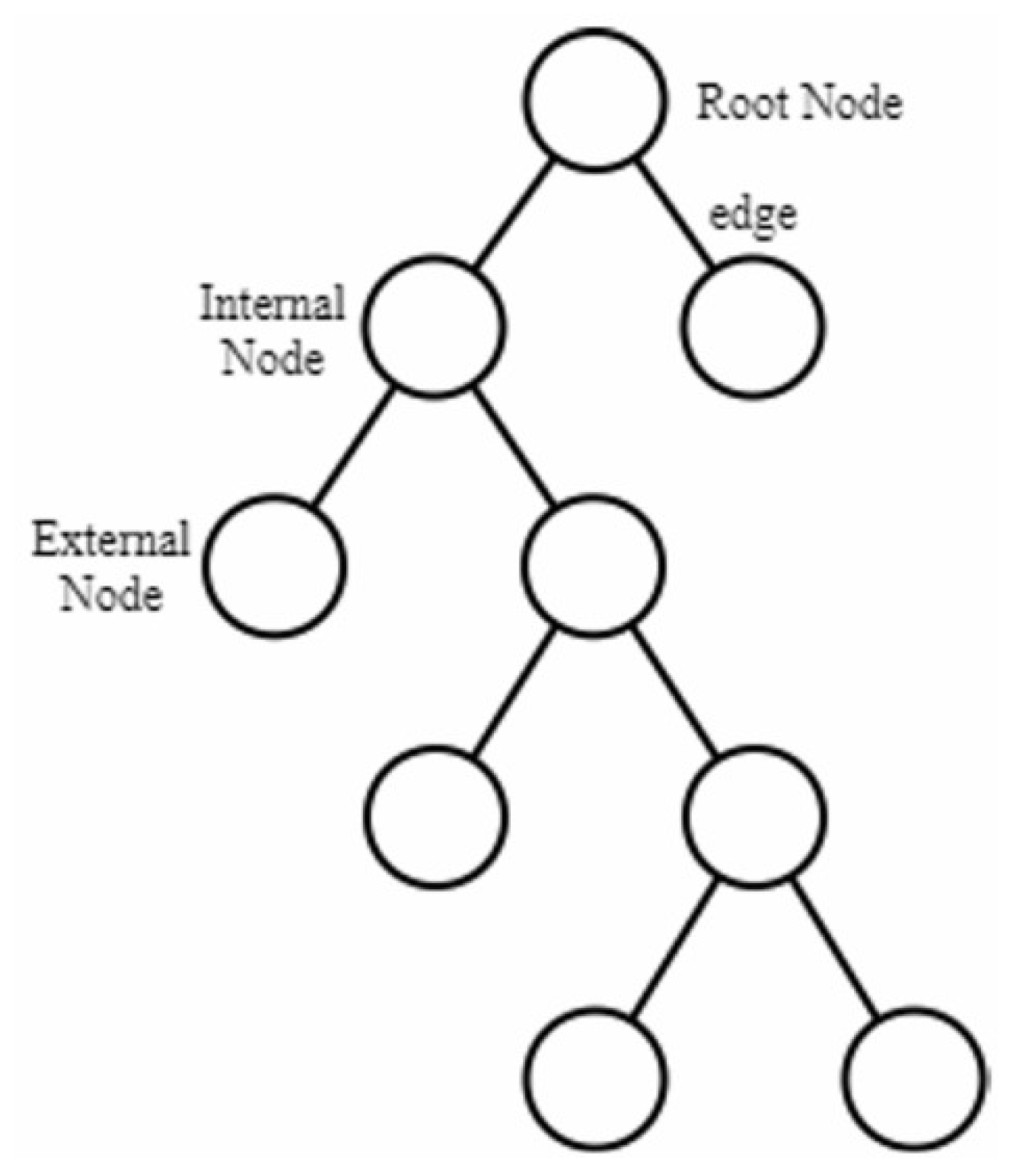
Figure 2.
Illustration of an autoencoder model
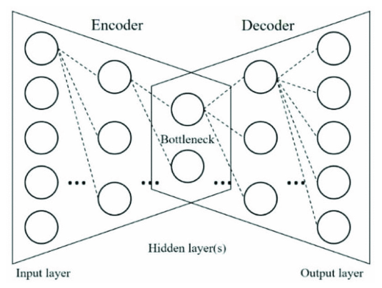
Figure 3.
Data distribution from raw data.
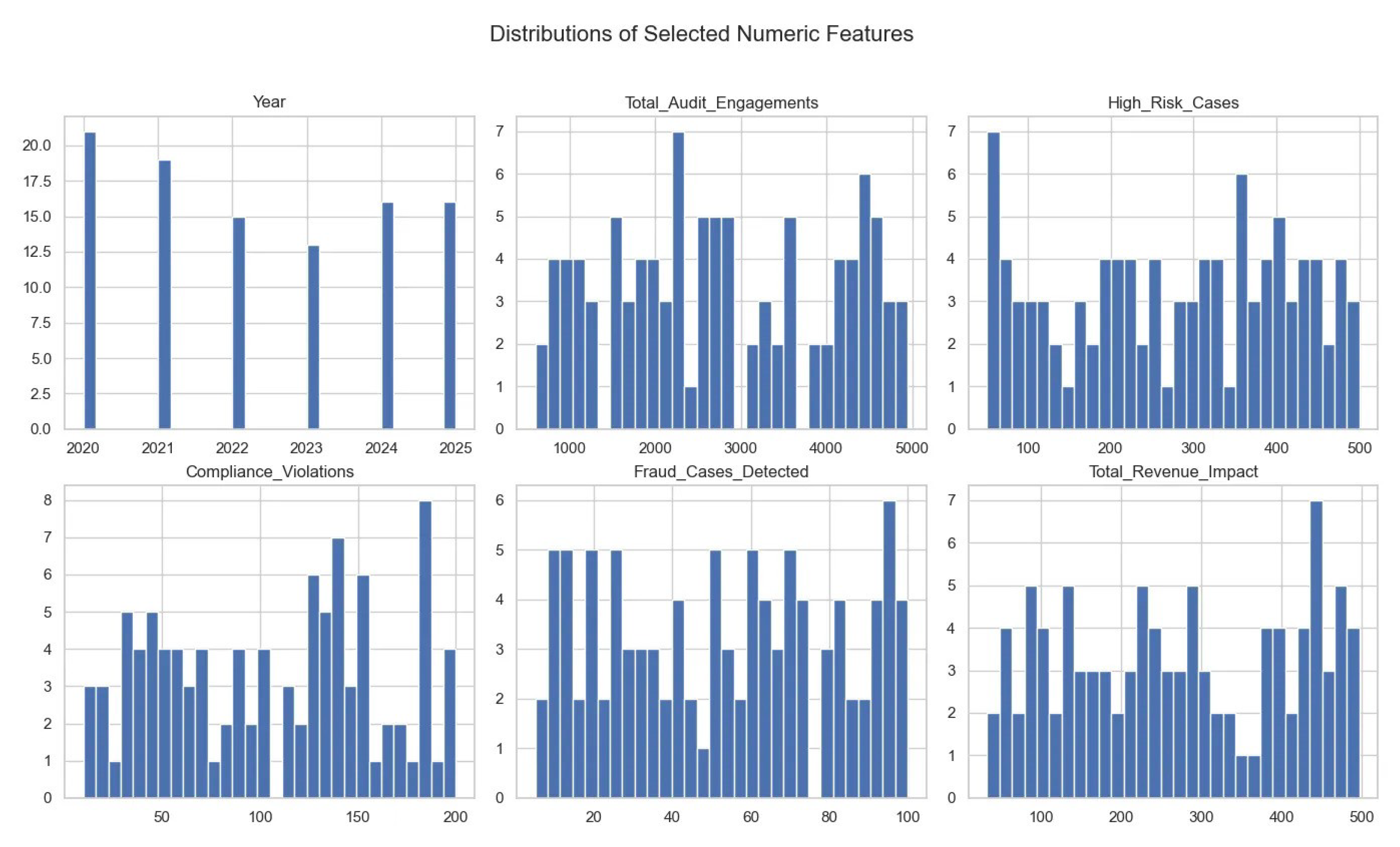
Figure 5.
feature-importance scores
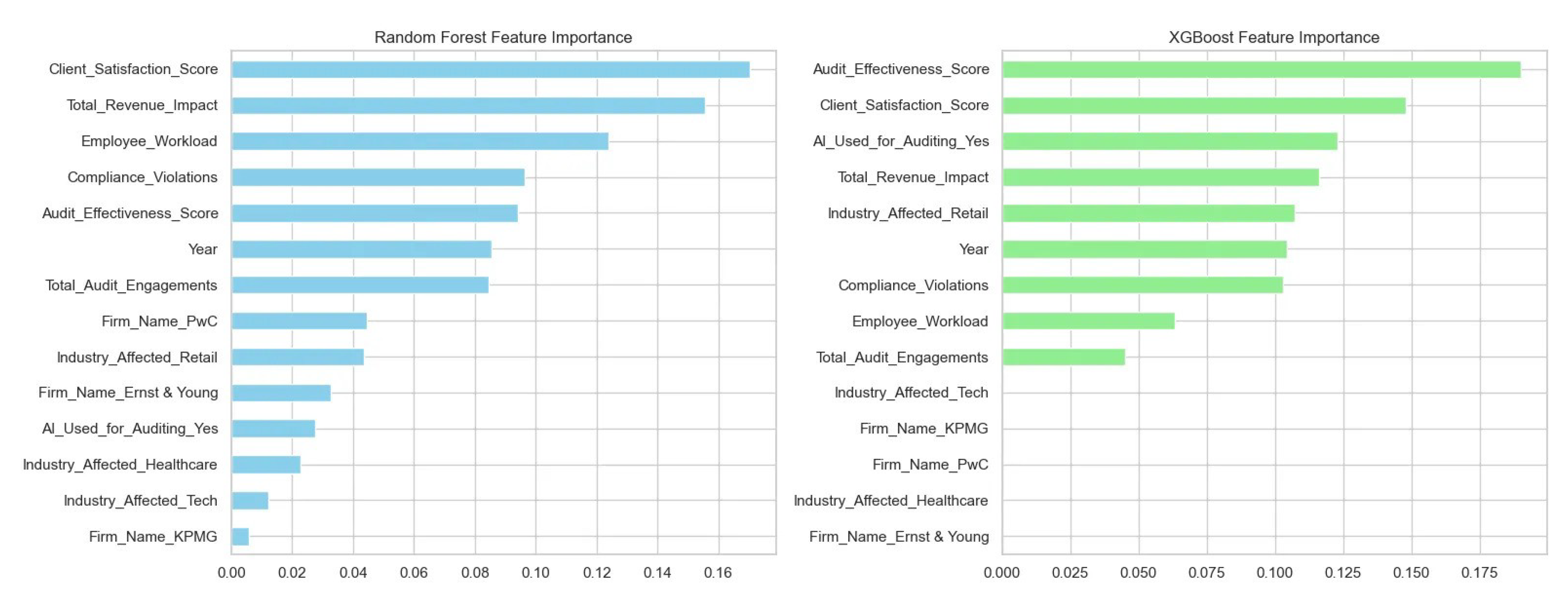
Figure 6.
feature-importance scores
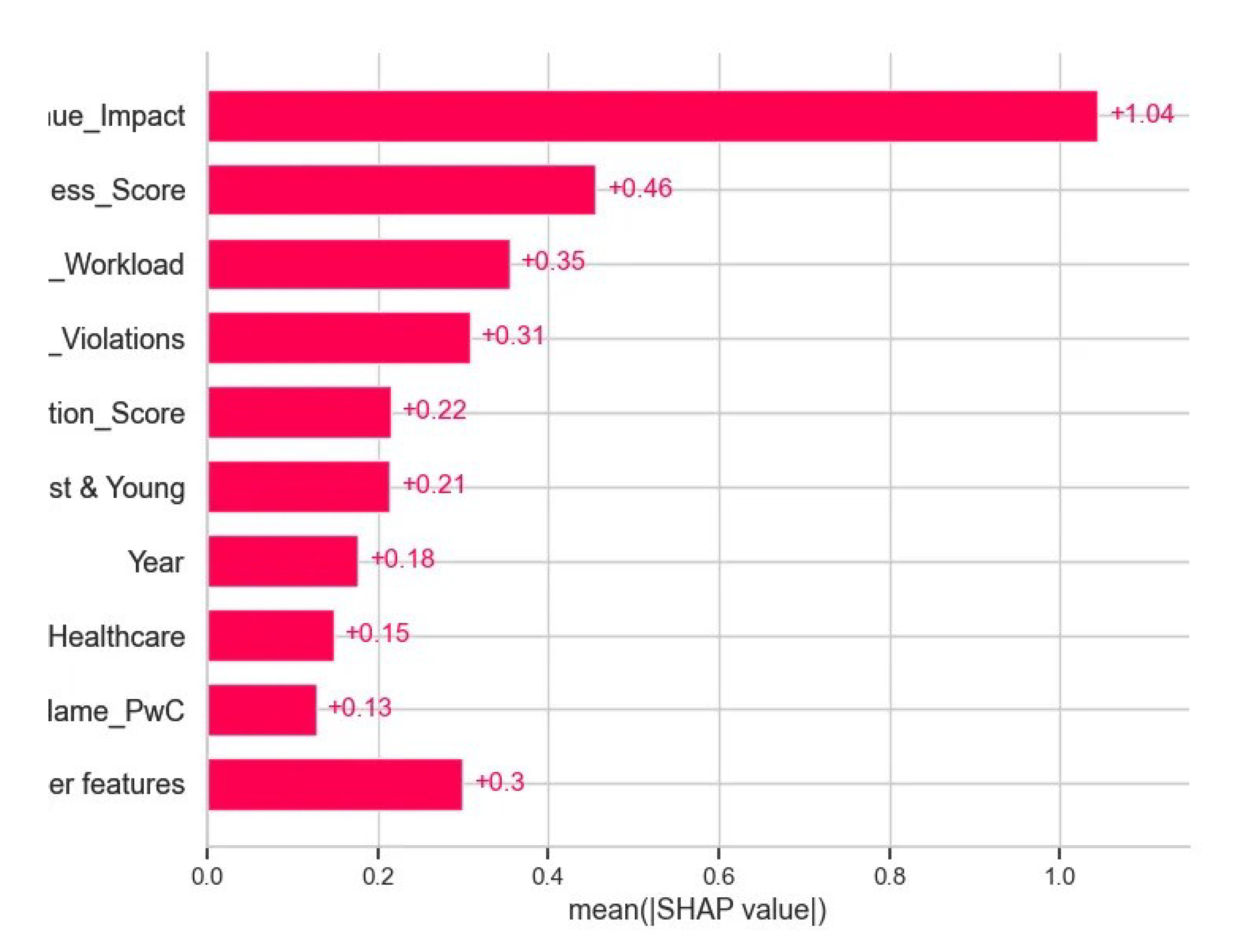
Figure 7.
base value = 2.953
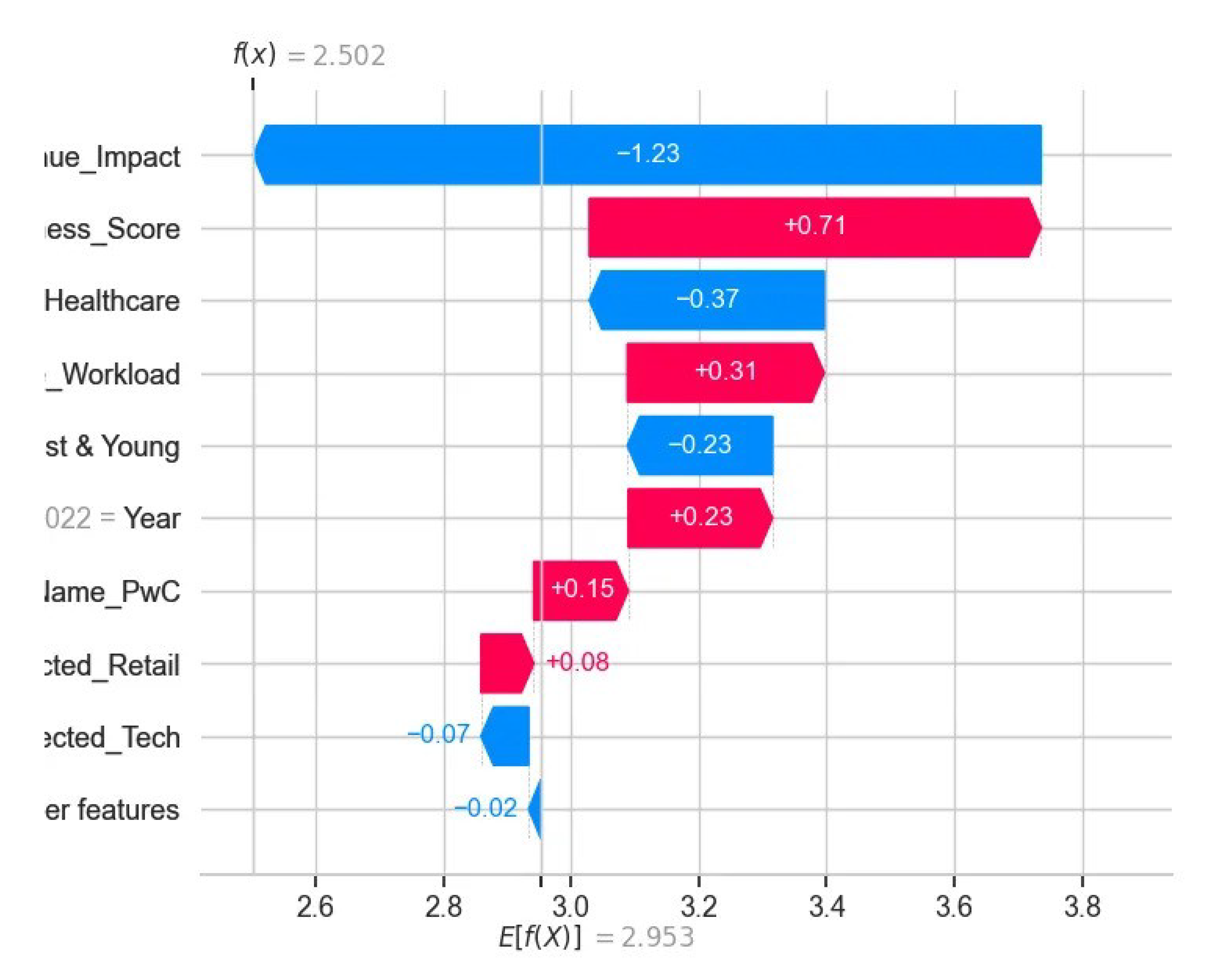
Table 1.
Summary of typical raw features in credit card datasets.
| Feature | Description |
| Transaction ID | Transaction identification number |
| Time | Date and time of the transaction |
| Account number | Identification number of the customer |
| Card number | Identification of the card |
| Transaction type | Internet, ATM or POS |
| Entry mode | Chip and pin or magnetic stripe |
| Amount | Amount of transaction |
| Merchant code | Identification of the merchant type |
| Merchant group | Merchant group identification |
| Country | Country of transaction |
| Country 2 | Country of residence |
| Type of card | Visa debit, MasterCard, American Express |
| Gender | Gender of the cardholder |
| Age | Age of the cardholder |
| Bank | Issuer bank of the card |
Table 2.
First five row of raw data.
| Year | Firm_Name | Total_Audit_Engagements | High_Risk_Cases | Client_Satisfaction_Score | |
| 2020 | PwC | 2829 | 51 | 8.4 | |
| 2022 | Deloitte | 3589 | 185 | 6.7 | |
| 2020 | PwC | 2438 | 212 | 6.2 | |
| 2021 | PwC | 2646 | 397 | 8.6 | |
| 2020 | PwC | 2680 | 216 | 6.8 |
Table 4.
Random Forest & XGBoost report.
| Metric / Class | Random Forest | XGBoost |
|---|---|---|
| False | ||
| Precision | 0.00 | 0.00 |
| Recall | 0.00 | 0.00 |
| 0.00 | 0.00 | |
| Support | 3 | 3 |
| True | ||
| Precision | 0.85 | 0.85 |
| Recall | 1.00 | 1.00 |
| 0.9189 | 0.9189 | |
| Support | 17 | 17 |
| Accuracy | 0.85 | 0.85 |
| Macro avg | ||
| Precision | 0.425 | 0.425 |
| Recall | 0.500 | 0.500 |
| 0.4595 | 0.4595 | |
| Support | 20 | 20 |
| Weighted avg | ||
| Precision | 0.7225 | 0.7225 |
| Recall | 0.8500 | 0.8500 |
| 0.7811 | 0.7811 | |
| Support | 20 | 20 |
Table 5.
Baseline performance result under seed 317325550.
| Seed | RF Accuracy | RF Recall | XGB Accuracy | XGB Recall |
| 317325550 | 0.85 | 1.00 | 0.85 | 1.0 |
Table 6.
CPU-optimized XGBoost Result
| Seed | XGB Accuracy | XGB Recall |
| 317325550 | 0.85 | 1.000000 |
| 640985805 | 0.85 | 1.000000 |
| 720367070 | 1.00 | 1.000000 |
| 742707455 | 0.95 | 1.000000 |
| 2045756861 | 0.85 | 0.894737 |
Disclaimer/Publisher’s Note: The statements, opinions and data contained in all publications are solely those of the individual author(s) and contributor(s) and not of MDPI and/or the editor(s). MDPI and/or the editor(s) disclaim responsibility for any injury to people or property resulting from any ideas, methods, instructions or products referred to in the content. |
© 2025 by the authors. Licensee MDPI, Basel, Switzerland. This article is an open access article distributed under the terms and conditions of the Creative Commons Attribution (CC BY) license (http://creativecommons.org/licenses/by/4.0/).
Copyright: This open access article is published under a Creative Commons CC BY 4.0 license, which permit the free download, distribution, and reuse, provided that the author and preprint are cited in any reuse.


