
Submitted:
11 September 2025
Posted:
12 September 2025
You are already at the latest version
Abstract
We introduce Experience-Based Pattern Matching (EBPM) as a biologically grounded alternative to Predictive Coding (PC) for rapid recognition and action. EBPM posits that familiar inputs trigger direct reactivation of multimodal engrams (sensory–motor–interoceptive–cognitive), avoiding continuous generative simulation and thereby reducing latency and compute. We provide a method-by-method comparison between EBPM and adjacent frameworks—attractor/Hopfield models, Complementary Learning Systems, hippocampal indexing (pattern completion/separation), HTM/sequence memory, Sparse Distributed Memory, memory-augmented neural networks (NTM/DNC), episodic control, metric-learning/prototypical networks, and PC/Active Inference—explicitly identifying (i) shared mechanisms, (ii) additions brought by each prior theory, and (iii) what EBPM adds beyond them. We further present DIME (Dynamic Integrative Matching and Encoding), a hybrid architecture that exploits EBPM’s one-shot recall on familiar inputs and falls back to PC under uncertainty or novelty via a lightweight controller. Across ANN benchmarks (MNIST, Fashion-MNIST, CIFAR-10) and a virtual robotics obstacle-course, EBPM consistently yields the lowest inference latency on familiar inputs, PC remains more robust to noise/novelty, and DIME adapts between them without sacrificing task performance. Finally, we formalize Algorithm 1 (EBPM) and map each step to prior art (sparse coding and assemblies; lateral inhibition/WTA; attractor-like selection; salience/LC-NE; Hebbian/STDP; hippocampal indexing), clarifying how EBPM integrates classic mechanisms into a unified, multimodal engram framework. The results motivate EBPM/DIME as neuro-plausible, energy-aware blueprints for hybrid AI and real-time robotic control.
Keywords:
EBPM
; multimodal engrams
; attractor networks
; Complementary Learning Systems
; hippocampal indexing
; HTM
; Sparse Distributed Memory
; memory-augmented neural networks
; episodic control
; metric learning
; Predictive Coding
; Active Inference
; DIME
; robotics
1. Introduction
Over the past three decades, the Predictive Coding (PC) paradigm has become one of the most influential theoretical frameworks in cognitive neuroscience. It posits that perception arises from a hierarchical process of top–down prediction generation, which is continuously compared with incoming sensory data, with the discrepancies propagated as prediction errors [1,2]. The PC model has successfully accounted for phenomena such as directed attention, multimodal integration, and the adaptive flexibility of the cortex, being closely linked to Bayesian mathematical principles and the “free energy principle” hypothesis [3].
Nevertheless, this framework presents both conceptual and practical limitations. First, PC entails a high computational and energetic cost, as it requires the continuous generation of internal predictions even in familiar contexts. Second, it assumes that perception is essentially a hypothesis-testing process, which does not accurately capture the rapid and reflexive responses observed at both neuronal and behavioral levels. Third, a substantial body of neurophysiological evidence suggests that recognition in familiar situations occurs through the direct reactivation of stored engrams, without an intermediate stage of generative simulation [4,5].
To address these limitations, we propose a new model—Experience-Based Pattern Matching (EBPM)—developed in this study. EBPM conceptualizes perception and action as the result of the direct activation of multimodal engrams (visual, auditory, motor, emotional), previously formed through experience. Each engram consists of elementary engram units, such as visual edges, motion fragments, or interoceptive cues, which can be reused and combined into complex networks. In this framework, novel stimuli initially activate these units, which may trigger a full familiar engram or partially activate several engrams. If none surpasses an activation threshold, attentional processes are engaged and new connections are formed—a process equivalent to biological supervised learning.
The EBPM model presents significant advantages over PC in familiar contexts: faster recognition, reduced energetic cost, and a natural alignment with neurophysiological data (Hebbian plasticity, lateral inhibition, direct memory reactivation). However, like PC, EBPM also has limitations: low robustness to noisy data and reduced flexibility when confronted with entirely novel stimuli.
Building on the observation that neither PC nor EBPM can fully account for all cognitive phenomena, this paper proposes a novel hybrid model—Dynamic Integrative Matching and Encoding (DIME). DIME integrates the two paradigms: it employs EBPM’s direct matching in familiar and rapid situations, but can recruit PC’s generative mechanisms when the context is ambiguous or incomplete. A dynamic control mechanism determines which pathway is dominant, ensuring both speed and efficiency, as well as flexibility and robustness. The general architecture of the DIME model is illustrated in Figure 3, which depicts the integration of EBPM and PC processing streams through a central control module.
The aim of this study is twofold: (i) to present the original EBPM model, together with its neurophysiological and algorithmic foundations, and (ii) to define the DIME architecture as an integrative solution between EBPM and PC. The work has an interdisciplinary character, with implications in cognitive neuroscience, artificial intelligence, and robotics. In addition, it proposes a methodological framework for validation through neuroimaging (fMRI, EEG/MEG), artificial neural network simulations, and robotic experiments, thereby providing both theoretical and applied relevance.
In addition to Predictive Coding, alternative frameworks have been proposed to explain recognition and cognition. Prior work on attractor-based memory models and predictive coding has argued for complementary roles of fast pattern completion and iterative inference. We build on this view by integrating both into a single decision process. However, these models typically focus either on abstract pattern completion without multimodality, or on purely Bayesian formulations without explicit engram reactivation. EBPM therefore differs in scope: it formalizes multimodal engrams and introduces a novelty-driven supervised-like learning process, providing a distinct alternative to both attractor and predictive theories.
See §2.3.6 for a method-by-method comparison between EBPM and attractor models, CLS, HTM, SDM, memory-augmented NNs, episodic control, metric-learning, and PC/Active Inference.
2. Materials and Methods
2.1. The Theoretical Framework of the EBPM Model
The Experience-Based Pattern Matching (EBPM) model, proposed in this paper, describes perception and action as the result of the direct activation of multimodal engrams. Each engram integrates:
- Sensory components (e.g., visual edges and colors, auditory timbres, tactile cues),
- Motor components (articular configurations, force vectors),
- Interoceptive and emotional components (visceral state, affective value),
- Cognitive components (associations, abstract rules).
These engrams are constructed through experience and consolidated by Hebbian plasticity and spike-timing-dependent plasticity (STDP) mechanisms [4,6]. They are composed of elementary sub-engrams (feature primitives), such as edge orientations or elementary movements, which can be reused in multiple combinations.
The EBPM Processing Stream:
- Stimulus activation – sensory input activates elementary engram units (sub-engrams) such as edges, textures, tones, motor or interoceptive signals.
- Engram co-activation – shared sub-engrams may partially activate multiple parent engrams in parallel.
- Scoring and aggregation – each parent engram accumulates an activation score based on the convergence of its sub-engrams.
- Winner selection – if a single engram surpasses the recognition threshold, it is fully activated and determines the output; if several engrames are partially active, the strongest one prevails through lateral inhibition.
- Novelty detection – if all activation scores remain below threshold, the system enters a novelty state: no complete engram is recognized.
- Attention engagement – attention is mobilized to increase neuronal gain and plasticity, strengthening the binding of co-active sub-engrams into a proto-engram.
- Consolidation vs. fading – if the stimulus/event is repeated or behaviorally relevant, the proto-engram is consolidated into a stable engram; if not, the weak connections gradually fade.
Formally, an engram unit (EU) can be defined as a feature vector EUi = [si,mi,ei,ci], where si denotes sensory primitives (edges, colors, timbres), mi denotes motor fragments (joint configurations, force vectors), ei captures interoceptive or affective values, and ci encodes cognitive associations or rules. A full engram is a sparse set {EU1,…EUn}, stabilized by Hebbian and spike-timing dependent plasticity (STDP). This formalization differentiates EBPM from generic episodic traces or attractor states by explicitly integrating multimodal dimensions.
Thus, EBPM accounts for rapid recognition in familiar contexts and provides a robust architecture for the storage of multimodal experiences.
This process is illustrated in Figure 1 and is consistent with the principles of Hebbian learning and sparse distributed coding [4,5]. Shows how sensory input activates atomic sub-engrams, which can either fully trigger a stored engram or partially activate multiple candidates. The winner-takes-all mechanism determines the output, while novelty detection engages supervised-like learning.
It is important to emphasize that in EBPM even novel or weakly familiar stimuli always activate sub-engrams (e.g., edges, textures, tones, tactile or interoceptive states). These activations may remain below the recognition threshold, being unable to complete any stable engram. In such cases, attention is mobilized, not only to enhance further sensory sampling but also to increase neuronal gain and plasticity, creating temporary proto-engrams by binding co-active sub-engrams according to the Hebbian rule (‘fire together, wire together’). If the stimulus or event is repeated or behaviorally relevant, these proto-engrams undergo consolidation into stable engrams; if the event does not recur, the weak connections gradually fade. Thus, attention serves a dual role: intensifying analysis of unfamiliar input while simultaneously facilitating the structural formation of new memory programs for future recognition.
2.2. The Theoretical Framework of Predictive Coding (PC)
Predictive Coding (PC) is an established framework according to which the cortex continuously generates top–down predictions, compares them with actual sensory data, and propagates the discrepancies as prediction errors [1,2]. PC has three fundamental elements:
- Internal generative models (hierarchical representations of the environment),
- Prediction errors (differences between input and predictions),
- Adaptive updating (learning through error minimization).
PC provides a good account of the brain’s flexibility in novel environments, its robustness to noise, and its capacity for cross-modal integration. However, its high energetic cost and long latencies make it less suitable for rapid responses.
This architecture is schematically represented in Figure 2, where predictions are transmitted top–down, while errors propagate bottom–up for adjustment. Illustrates the generative top–down predictions, the comparison with incoming sensory data, and the propagation of prediction errors upwards in the cortical hierarchy [1,3].
2.3. Comparison of EBPM and PC
2.3.1. Theoretical Foundation
Over the past two decades, Predictive Coding (PC) has become the dominant framework for explaining perception and cognition. PC posits that the nervous system constructs hierarchical generative models that continuously predict sensory input and update these models through the minimization of prediction errors.
In contrast, the EBPM model proposed here argues that perception and action rely on the direct activation of pre-existing multimodal engrams, without requiring the active generation of predictions. EBPM is grounded in the principle that recognition is determined by the similarity between input and stored patterns; only when the input is insufficient to activate an existing engram do attentional processes and supervised learning come into play.
Thus, the fundamental difference is that PC operates through predictive reconstruction, whereas EBPM operates through direct matching.
2.3.2. Processing Dynamics in the Two Models
Predictive Coding (PC)
- The brain generates hierarchical top–down predictions.
- Sensory input is compared with predictions.
- Prediction errors are transmitted upward and correct the internal model.
- Perception arises as the result of minimizing the difference between prediction and input.
EBPM
- The input activates elementary engram units.
- The elementary engram units simultaneously activate multiple engrams.
- Through lateral inhibition, the most active engram prevails.
- If no winner exceeds the threshold, attention is triggered and a new engram is formed.
- Perception is the complete reactivation of a pre-existing network, not a reconstruction process.

Table 1.
Extended comparison between Predictive Coding (PC) and Experience-Based Pattern Matching (EBPM), with explicit treatment of novelty, attention, and new engram formation.
Table 1.
Extended comparison between Predictive Coding (PC) and Experience-Based Pattern Matching (EBPM), with explicit treatment of novelty, attention, and new engram formation.
| Aspect | Predictive Coding (PC) | Engram-Based Program Model (EBPM) |
|---|---|---|
| Basic principle | Predictions compared with input; error is propagated. | Recognition through engrames composed of reusable sub-engrams; full activation only for familiar stimuli. |
| Partial activation | - | Partial/similar stimuli → shared sub-engrams are activated; multiple engrams become partially active. |
| Selection | - | Lateral inhibition: the engram with the most complete activation prevails. |
| Novelty / unfamiliarity | Unclear how new representations are detected and formed | If all engrames remain below threshold: sub-engrams are active, but no parent engram is completed → novelty state. Attention is engaged. |
| Formation of new engrames (role of attention) | Does not specify a concrete biological mechanism. | Automatic (“fire together, wire together”): in the novelty state, attention increases neuronal gain and plasticity; co-active sub-engrams are bound into a proto-engram. Without repetition: the linkage fades/does not finalize. With repetition: it consolidates into a stable engram. |
| Signaling absence | Postulates “omission error” (biologically problematic). | No “negative spike.” Silence at parent-engrams level + fragmentary activation of sub-engrams defines novelty; attention manages exploration and learning. |
| Neuronal logic | Requires an internal comparator/explicit error signals. | Pure spike/silence + lateral inhibition + co-activation-dependent plasticity; attention sets the learning threshold. |
In EBPM, novelty does not mean absence of activation, but rather fragmentary activation: elementary sub-engrams (edges, textures, sounds, interoceptive states, etc.) respond, yet no parent engram reaches the recognition threshold. This state triggers attention mechanisms, which increase neuronal gain and synaptic plasticity on the relevant circuits. According to the principle ‘fire together, wire together’, co-active sub-engrams are linked into a proto-engram. If the stimulus/event is repeated (or remains behaviorally relevant), these linkages are consolidated into a stable engram; if not, they remain weak and fade. Thus, attention not only collects additional data, but also guides and accelerates the very process of inscribing new engrams.”
2.3.3. Comparative Advantages and Limitations
Table 2.
a. Conceptual Differences between EBPM and PC.
| Domain | EBPM | PC Prediction |
|---|---|---|
| Central Mechanism | Direct Activation of Multimodal Engrams | Continuous generation and updating of predictions |
| The Role of Prediction | Non-existent; only goal-driven sensitization | Fundamental for processing |
| Recognition Speed | Instantaneous for familiar stimuli | Slower, requires iterative computation |
| Energy Efficiency | High (without generative simulation) | Lower (increased metabolic cost) |
| Attention Control | Goal-driven (sensitization of relevant networks) | Through the magnitude of prediction errors |
| Biological Plausibility | Supported by studies on engrams and inhibition | Supported by cortical predictive microcircuits |
| Typical Application Domains | Rapid recognition, episodic memories, reflexes | Perception in ambiguous or noisy conditions |
Table 2.
b. Conceptual differences extended with related models.
| Domain | EBPM | PC | Similar existing theories |
|---|---|---|---|
| Central Mechanism | Direct multimodal engram activation | Generative predictive coding | Hopfield attractors, episodic replay |
| Recognition Speed | Fast, one-step match | Iterative, slower | Fast (pattern completion) |
| Energy Efficiency | High, no generative loop | Low, high metabolic demand | Variable |
| Flexibility | Limited to stored engrams | High, reconstructive | Active inference |
| Biological Plausibility | Supported by engram studies | Supported by cortical microcircuits | Both partially supported |
2.3.4. Divergent Experimental Predictions
Table 3.
Comparative Predictions: EBPM vs. PC.
| Domain | EBPM Prediction | PC Prediction | Testable through |
|---|---|---|---|
| fMRI (similarity analysis) | Recognition = reactivation of storage networks | Anticipatory activation in higher cortical areas | fMRI + RSA |
| EEG/MEG (latency) | Rapid recognition of familiar patterns | Longer latencies due to generative processing | EEG/MEG |
| Cue-based recall | A partial cue reactivates the entire engram | The cue triggers generative reconstruction | Behavioral and neurophysiological studies |
| Robotic Implementation | Faster execution of learned procedures | Better adaptive reconstruction with incomplete data | AI/Robotics Benchmarks |
2.3.5. Interpretive Analysis
- EBPM better explains rapid recognition, complex reflexes, and sudden cue-based recall.
- PC is superior in situations with incomplete or ambiguous data, due to its generative reconstruction capability.
- The two models are therefore complementary, each having its own set of advantages and limitations.
This observation sets the stage for an integrative model (DIME), which combines the speed and efficiency of EBPM with the flexibility of PC.
2.3.6. EBPM vs. Related Theories — Method-by-Method Comparison
Context. EBPM (direct reactivation of multimodal engrams) was defined in §2.1 and contrasted with Predictive Coding (PC) in §2.2–§2.3; DIME integrates them in §2.4. Below we align EBPM against adjacent frameworks, highlighting (i) what is identical, (ii) what each prior method adds, and (iii) what EBPM adds.
Table 4.
Side-by-side comparison (operational summary).
| Method / Framework | What the method does | Identical to EBPM | What it adds vs. EBPM | What EBPM adds |
|---|---|---|---|---|
| Hopfield / Attractor networks [7] | Recurrent dynamics converge to stored patterns (content-addressable recall from partial cues). | Pattern completion from partial input; competition among states. |
Explicit energy formalism; well-characterized attractor dynamics. |
Explicit multimodality (sensory–motor–affective–cognitive) and engram units beyond binary patterns. |
| CLS — Complementary Learning Systems (hippocampus fast; neocortex slow) [8] | Episodic rapid learning + slow semantic consolidation. | Separation of “fast vs. slow” memory routes. | System-level transfer between stores. | EBPM is operational in real time via direct matching; no mandatory inter-system consolidation for recognition. |
| Hippocampal indexing: pattern completion/separation [9,10] | Hippocampus indexes episodes; CA3 supports completion, DG supports separation. | Fast episodic reactivation from indices; completion logic. | Fine neuro-anatomical mapping (CA3/DG) with predictions. | EBPM generalizes to neocortex and to multimodal action-oriented engrams, not only episodic replays. |
| Exemplar / Instance-Based (GCM; Instance Theory) [11,12] | Decisions by similarity to stored instances; latencies fall with instance accrual. | Direct “match to memory” with similarity score. | Quantitative psychophysics of categorization and automatization. | EBPM includes motor/interoceptive bindings and neuronal lateral inhibition/WTA selection. |
| Recognition-by-Components (RBC) [13] | Object recognition via geons and relations. | Sub-engrams akin to primitive features. | Explicit 3D structural geometry. | EBPM is not vision-limited; covers sequences/skills and affective valence. |
| HTM / Sequence Memory (cortical columns) [5] | Sparse codes, sequence learning, local predictions. | Reuse of sparse distributed codes; sequence handling. | Continuous prediction emphasis. | EBPM does not require continuous generative prediction; for familiar inputs it yields lower latency/energy via direct recall. |
| Sparse Distributed Memory (SDM) [14] | Approximate addressing in high-D sparse spaces; noise-tolerant recall. | Proximity-based matching in feature space. | Abstract memory addressing theory. | EBPM specifies engram units and novelty/attention gating with biological microcircuit motifs. |
| Memory-Augmented NNs (NTM/DNC)[15,16] | Neural controllers read/write an external memory differentiably. | Key-based recall from stored traces. | General algorithmic read/write; task-universal controllers. | EBPM is bio-plausible (engram units; STDP-like plasticity) without opaque external memory. |
| Episodic Control in RL [17] | Policies exploit episodic memory for rapid action. | Fast reuse of familiar episodes. | RL-specific credit assignment and returns. | EBPM operates for perception and action with multimodal bindings. |
| Prototypical / Metric-Learning (few-shot) [18] | Classify by distance to learned prototypes in embedding space. | Prototype-like matching ≈ EBPM encoder + similarity. | Episodic training protocols; few-shot guarantees. | EBPM grounds the embedding in neuro-plausible engrams + inhibition, not just vector spaces. |
| Predictive Coding / Active Inference [1], [2,3,19,20] | Top-down generative predictions + iterative error minimization. | Shares attentional modulation and context use. | Robust reconstruction under missing data via generative loops. | EBPM delivers instant responses on familiar inputs (no iterative inference) with lower compute/energy; DIME then falls back to PC for novelty. |
Algorithm 1 — EBPM (step-by-step) with prior-art mapping
- Extract low-level primitives (edges, textures, timbre, phonemes).
- 2.
- Activate candidate multimodal Engram Units (EUs) from those primitives.
↳ Cell assemblies / neural assemblies concepts. [4]
- 3.
- Spread + compete among candidate EUs with lateral inhibition / WTA.
- 4.
- Select the winner (fully activated engram) → recognition / action trigger.
- 5.
- Familiarity/novelty test (no clear winner → novelty branch).
- 6.
- Rapid plasticity (Hebb/STDP-like) to form/adjust new or refined engrams.
↳ Hebbian/STDP literature. [6]
- 7.
- Bind multimodal facets (sensory–motor–affective–cognitive) within the engram; optional hippocampal indexing for episode-level links.
- 8.
- Real-time reuse: for familiar inputs, jump straight to Steps 3–4 (no generative loop).
2.3.7. Distinctive Contributions of EBPM (Beyond Attractors/CLS/HTM/PC)
While Section 2.3.6 aligned EBPM with adjacent frameworks, here we summarize the contributions that are unique or substantially sharpened by EBPM:
- Multimodal Engram as the Computational Unit. EBPM defines an engram as a compositional binding of sensory, motor, interoceptive/affective, and cognitive facets. This goes beyond classic attractor networks (binary pattern vectors) and metric-learning embeddings by specifying the unit of recall and action as a multimodal assembly.
- Novelty-first Decision with Explicit Abstention. By design, EBPM yields near-zero classification on truly novel inputs. Partial activation of sub-engrams is treated as a reliable novelty flag—not as a misclassification. This sharp separation of recognition versus novelty is absent from PC’s iterative reconstruction loop and from generic prototype schemes.
- Attention-gated Proto-Engram Formation. EBPM assigns a concrete role to attention and neuromodulatory gain (e.g., LC-NE) in binding co-active sub-engrams into a proto-engram during novelty, followed by consolidation. This specifies “when and how new representations form” more explicitly than attractors/CLS/HTM.
- Real-time Reuse without Iterative Inference. For familiar inputs, EBPM supports one-step reactivation of stored engrams (winner selection via lateral inhibition), avoiding costly predictive iterations. This explains ultra-fast recognition and procedural triggering in overlearned contexts.
- Integration-readiness via DIME. EBPM is not an isolated alternative: the DIME controller provides a formal arbitration (α) that privileges EBPM under high familiarity and shifts toward PC under uncertainty, yielding a principled hybrid.
2.4. The DIME Integrative Model
To overcome the limitations of both paradigms, we propose DIME (Dynamic Integrative Matching and Encoding)—a model that combines EBPM’s direct matching with PC’s generative prediction.
Principles:
- Dual-path processing: sensory input is processed simultaneously through direct engram matching (EBPM) and top–down prediction (PC).
- Dynamic controller: a central mechanism evaluates the context (level of familiarity, uncertainty, noise) and selects the dominant pathway.
- Adaptive flexibility: in familiar environments → EBPM becomes dominant; in ambiguous environments → PC is engaged.
Algorithmically, DIME can be formulated as follows:
where S(t) is stimulus, M_EBPM and M_PC are the outputs of the two models, and α(t)∈[0,1] is the adaptive weighting determined by the controller.
O(t) = α(t)⋅M_EBPM(S(t)) + (1−α(t))⋅M_PC(S(t))
The adaptive controller α(t) is defined as:
where F represents familiarity (cosine similarity between input and stored engrams), U represents uncertainty (variance of predictive reconstruction), and τF, τU are sensitivity thresholds. Parameters a and b determine the gain of the controller, and σ is the logistic activation. Biologically, F may correspond to hippocampal pattern-completion signals, while U aligns with prefrontal/parietal uncertainty estimation.
α(t) = σ[a(F − τF) − b(U − τU)]
Implementation note (ANN runs in §3). In our implementation we instantiate Eq. (2) as
where F^ is a calibrated familiarity signal derived from EBPM as the maximum cosine similarity to class prototypes, standardized on the familiar validation set (μ,σ), shifted by a small thr_shift, and passed through a logistic with gain (gain_fam). U is the normalized Shannon entropy of the PC predictive distribution U = H(p) / log10. This absorbs the thresholds in Eq. (2) into the calibration of F and the scale of U, yielding a simple F^ − U arbitration used in all reported ANN experiments.
α = σ(g⋅(F^ − U))
The general architecture of the DIME model is presented in Figure 3, which illustrates the integration of the EBPM and PC processing streams through a central control module [22,26]. Diagram of the dual-pathway system: EBPM (direct engram reactivation) vs. PC (generative prediction), with a dynamic controller weighting both outputs depending on familiarity and uncertainty.
2.5. Methodology of Experimental Validation
Testable Predictions and Analysis Plan
We highlight a set of testable predictions that distinguish EBPM from PC and can be empirically evaluated:
- H1 (EEG/MEG latency). EBPM-dominant trials (familiar stimuli) yield shorter recognition latencies (≈200–300 ms) compared to PC-dominant trials (≈350–450 ms). We base the ≈200–300 ms range on recent EEG evidence indicating that recognition memory signals emerge from around 200 ms post-stimulus across diverse stimulus types [27].
- H2 (fMRI representational similarity). EBPM produces higher RSA between learning and recognition patterns in hippocampal/cortical regions; PC shows anticipatory activation in higher areas under uncertainty.
- H3 (Cue-based recall completeness). Partial cues reinstantiate full engram patterns under EBPM, while PC engages reconstructive dynamics without full reinstatement.
- H4 (Behavioral/robotic efficiency). Under stable familiarity, EBPM leads to lower inference time and energy cost than PC; under novelty/noise, DIME shifts toward PC to preserve robustness.
- H5 (NE-gain modulation). Pupil-indexed or physiological proxies of LC-NE correlate with novelty detection and proto-engram formation during EBPM-dominant novelty trials.
These hypotheses are structured to allow empirical falsification and ensure that EBPM/DIME is not merely a descriptive framework, but a model with measurable consequences.
To test the EBPM, PC, and DIME hypotheses, we propose a multi-level approach:
-
Neuroimaging:
- fMRI (representational similarity analysis, RSA) → measures the overlap of patterns between learning and recognition.
- EEG/MEG → measures recognition latencies (EBPM ≈ shorter, PC ≈ longer).
-
Computational simulations:
- Artificial neural networks inspired by EBPM vs. PC.
- Comparison of inference times and computational cost.
-
Robotic experiments:
- Implementation in visuomotor control.
- Measurement of reaction times and energy consumption in navigation tasks.
This methodology enables the integrated testing of theoretical hypotheses and the assessment of the practical applicability of the DIME model.
The methodological structure is illustrated in Figure 4: (i) neuroimaging establishes the cortical dynamics associated with EBPM vs. PC, (ii) simulations on artificial neural networks (ANNs) compare execution times and noise robustness for the two models, and (iii) robotic tests assess practical applicability in real-time visuomotor control tasks. Such a combined approach is recommended in the computational neuroscience literature to triangulate and validate the proposed mechanisms [28]. Overview of the three validation layers: (i) neuroimaging (fMRI RSA, EEG/MEG latency), (ii) ANN simulations, (iii) robotic implementations.
2.6. ANN Simulation Protocol
Datasets. MNIST, Fashion-MNIST, and CIFAR-10. Familiar classes: 0–7; novel classes: 8–9. Inputs are converted to grayscale and resized to 28×28 for MNIST/F-MNIST; CIFAR-10 uses standard 32×32 RGB but is projected to the model’s input space as in our code.
Noise. We evaluate four scenarios per dataset: Familiar-Clean, Familiar-Noisy, Novel-Clean, Novel-Noisy. For the Noisy conditions we add zero-mean Gaussian noise with standard deviation σ relative to pixel values in [0,1], followed by clamping to [0,1]. MNIST/Fashion-MNIST: σ = 0.30. CIFAR-10: σ = 0.15. No additional corruptions are used.
EBPM. A prototype-based encoder maps inputs to a normalized embedding; class logits are cosine similarities to learned class prototypes (familiar classes).
PC (predictive coding). An autoencoder with a classifier at the latent layer; inference uses K = 10 gradient steps with step size η=0.1 to reduce reconstruction error before classification.
DIME. We use two integration strategies:
- (i)
- DIME-Prob (probability-level fusion): p = α·p_EBPM + (1−α)·p_PC, with α driven by a familiarity score calibrated on familiar validation data. On CIFAR-10 we tune {gain = 4.0, thr_shift = 0.75, T_EBPM = 6.0, T_PC = 1.0}.
- (ii)
- (ii) DIME-Lazy (runtime-aware gating, used in robotics): δ = mean(|I_t − I_{t−1}|). If δ ≤ 0.004 → EBPM-only; if δ ≥ 0.015 → PC-only; otherwise fuse with fixed α = 0.65.
Metrics. Top-1 accuracy and latency (ms/ex.) measured on the same GPU (Tesla T4; PyTorch 2.8.0 + cu126). We provide all raw TXT/CSV outputs in the Supplementary package (see Data & Code Availability).
Unless otherwise noted, results are reported for a single deterministic seed (SEED = 42) with CuDNN determinism enabled; numbers are point estimates per test set. Multi-seed statistics are left to future work.
3. Results
Preface — Scope of the Simulations (Proof-of-Concept)
We emphasize that the simulations reported in §3 are minimal proof-of-concept instantiations designed to demonstrate that the EBPM/DIME framework can be implemented and exercised end-to-end. The core contribution of this paper is the conceptual and architectural proposal, not exhaustive benchmarking. Accordingly, MNIST/Fashion-MNIST/CIFAR-10 and the PyBullet obstacle course serve to illustrate feasibility and the predicted trade-offs: speed and efficiency for EBPM on familiar inputs, robustness for PC under noise/novelty, and adaptive arbitration for DIME. Comprehensive large-scale evaluations and richer robotic tasks are deferred to future work (see §4.5).
3.1. ANN Simulations on Familiar vs. Novel Splits
We evaluated EBPM (prototype matching), PC (predictive autoencoder with iterative latent inference, K=10, η=0.1), and DIME (fusion of EBPM and PC) on MNIST, Fashion-MNIST, and CIFAR-10 under four scenarios: Familiar-Clean, Familiar-Noisy (Gaussian σ as in the code), Novel-Clean and Novel-Noisy. Familiar classes were 0–7; novel were 8–9.
Noise parameterization. For completeness, the Noisy conditions use zero-mean Gaussian noise with σ relative to [0,1] pixel values, followed by clamping: MNIST/Fashion-MNIST σ = 0.30; CIFAR-10 σ = 0.15.
- Metrics: top-1 accuracy, latency (ms/ex.), and for DIME the mean controller weight ᾱ where applicable.
- These results support the complementarity… (see Section 2.6).
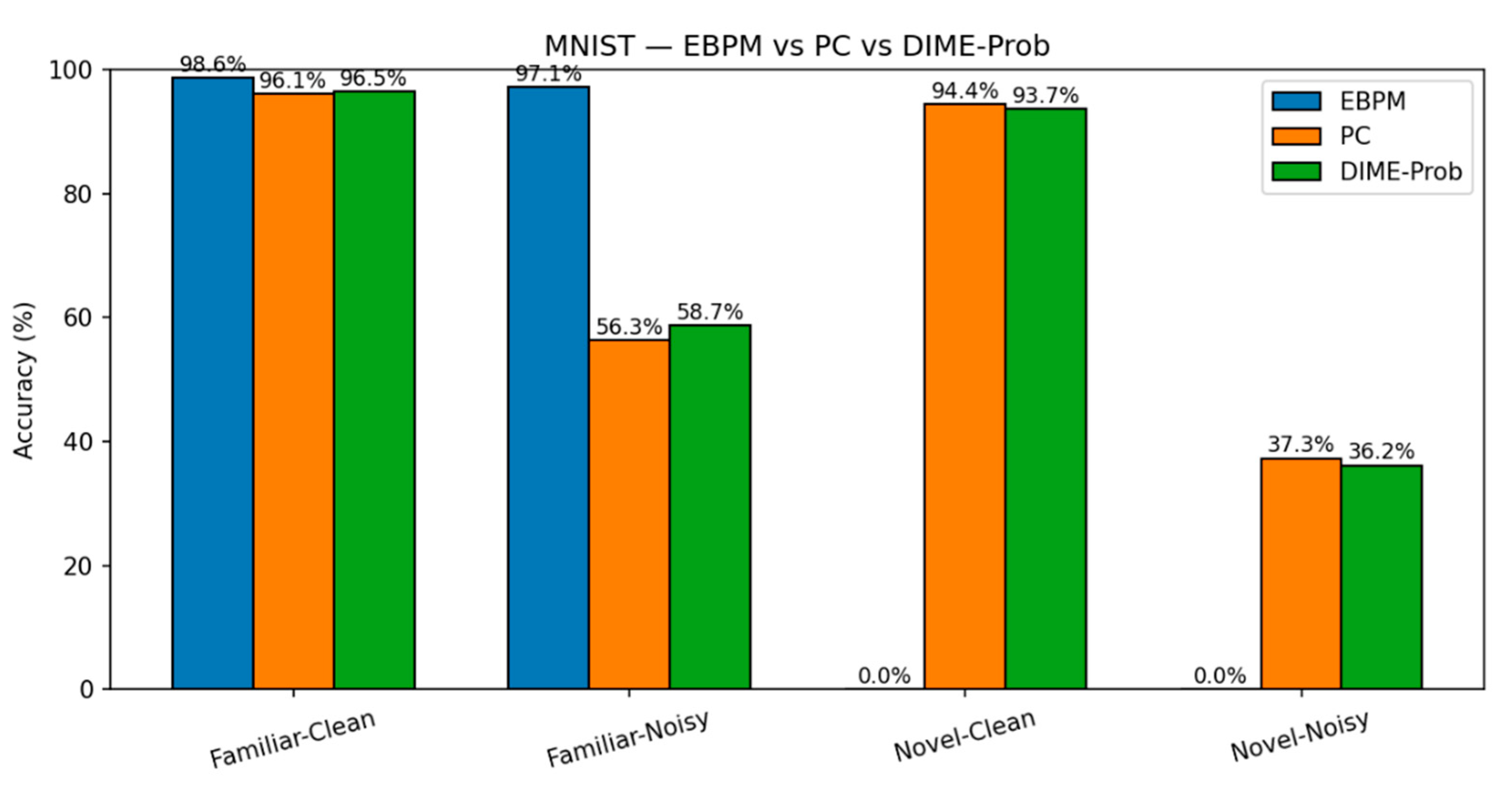
MNIST. EBPM is near-optimal on familiar inputs but, by design, does not classify novel digits (≈0%). This reflects its novelty-flagging mechanism: sub-engrams are activated but do not complete a full engram, signaling unfamiliarity rather than misclassifying. PC is slower but generalizes better to novelty, while DIME adapts by following EBPM on familiar inputs and engaging PC under uncertainty.
Key numbers from our runs:
- EBPM — Familiar-Clean: 98.63%, 0.100 ms/ex; Familiar-Noisy: 97.13%, 0.132 ms/ex; Novel: 0.0%.
- PC — Familiar-Clean: 96.11%, 0.281 ms/ex; Familiar-Noisy: 56.28%, 0.177 ms/ex; Novel-Clean: 94.40%, 0.154 ms/ex; Novel-Noisy: 37.27%, 0.188 ms/ex.
- DIME (adaptive) — Familiar-Clean: 98.63%, 0.247 ms/ex, ᾱ = 0.993; Familiar-Noisy: 96.93%, 0.188 ms/ex, ᾱ = 0.974; Novel≈0% (as EBPM dominates unless fused).
- DIME-Prob (probability-level fusion) — Familiar-Clean: 96.47%, 0.264 ms; Familiar-Noisy: 58.68%, 0.208 ms; Novel-Clean: 93.65%, 0.197 ms; Novel-Noisy: 36.16%, 0.239 ms.
- Fashion-MNIST. Trends are similar to MNIST, with a larger familiar/noise gap.
- EBPM — Familiar-Clean: 82.56%, 0.101 ms; Familiar-Noisy: 52.35%, 0.139 ms; EBPM reports ≈0% accuracy on novel inputs, consistent with its design as a novelty detector: sub-engrams activate but do not yield a full engram. This produces an explicit novelty signal, rather than a forced classification.
- PC — Familiar-Clean: 83.14%, 0.182 ms; Familiar-Noisy: 50.45%, 0.238 ms; Novel-Clean: 96.50%, 0.160 ms; Novel-Noisy: 97.00%, 0.203 ms.
- DIME (adaptive) — Familiar-Clean: 84.14%, 0.133 ms, ᾱ = 0.536; Familiar-Noisy: 51.31%, 0.170 ms, ᾱ = 0.221; Novel-Clean: 81.10%, 0.165 ms, ᾱ = 0.506; Novel-Noisy: 97.10%, 0.213 ms, ᾱ = 0.443.
CIFAR-10.
- EBPM — Familiar-Clean: 70.42%, 0.198 ms; Familiar-Noisy: 42.67%, 0.192 ms; Novel: 0%.
-
PC — Familiar-Clean: 65.99%, 0.477 ms; Familiar-Noisy: 27.15%, 0.478 ms; Novel-Clean: 83.10%, 0.536 ms; Novel-Noisy: 50.95%, 0.548 ms.
- DIME-Prob (best tuned) — Familiar-Clean: 68.31%, 0.529 ms; Familiar-Noisy: 30.38%, 0.535 ms; Novel-Clean: 62.50%, 0.609 ms; Novel-Noisy: 38.05%, 0.675 ms.
Remark. On Fashion-MNIST, PC shows a slight reversal—Novel-Noisy (97.00%) marginally exceeds Novel-Clean (96.50%). With σ = 0.30 Gaussian noise (clamped to [0,1]), this acts as a mild regularizer that attenuates high-frequency artifacts for some classes, yielding a small improvement within the expected variance band. The effect is not observed on MNIST or CIFAR-10 and does not change our overall conclusion (EBPM excels on familiar; PC on novel; DIME trades off adaptively)
These results support the complementarity of EBPM and PC and the usefulness of DIME as a context-adaptive integration. In particular, EBPM’s absence of classification on novel inputs should be read as a feature rather than a flaw: it provides a reliable novelty flag that complements PC’s generative reconstruction. This complementarity underlies the adaptive trade-offs realized in DIME.
Table 5.
a. MNIST (single-seed, SEED=42).
| Model | Familiar-Clean (acc / ms) |
Familiar-Noisy (acc / ms) | Novel-Clean (acc / ms) |
Novel-Noisy (acc / ms) |
ᾱ |
|---|---|---|---|---|---|
| EBPM | 98.63% / 0.100 | 97.13% / 0.132 | 0.00%* / 0.126 | 0.00%* / 0.161 | - |
| PC | 96.11% / 0.281 | 56.28% / 0.177 | 94.40% / 0.154 | 37.27% / 0.188 | - |
| DIME | 98.63% / 0.247 | 96.93% / 0.188 | 0.00% / 0.135 | 0.00% / 0.289 | 0.99 / 0.97 / – / – |
| DIME-Prob | 96.47% / 0.264 | 58.68% / 0.208 | 93.65% / 0.197 | 36.16% / 0.239 | 0.61/ 0.38/ 0.41/ 0.23 |
* For EBPM, Novel = 0% indicates explicit novelty detection (no engram completed), not misclassification. Sub-engrams are activated but recognition is withheld until learning occurs.
Table 5.
b. Fashion-MNIST.
| Model | Familiar-Clean (acc / ms) |
Familiar-Noisy (acc / ms) | Novel-Clean (acc / ms) |
Novel-Noisy (acc / ms) |
ᾱ |
|---|---|---|---|---|---|
| EBPM | 82.56% / 0.101 | 52.35% / 0.139 | 0.00% / 0.147 | 0.00% / 0.174 | - |
| PC | 83.14% / 0.182 | 50.45% / 0.238 | 96.50% / 0.160 | 97.00% / 0.203 | - |
| DIME | 84.14% / 0.133 | 51.31% / 0.170 | 81.10% / 0.165 | 97.10% / 0.213 | 0.54 / 0.22 / 0.51 / 0.44 |
Table 5.
c. CIFAR-10.
| Model | Familiar-Clean (acc / ms) |
Familiar-Noisy (acc / ms) |
Novel-Clean (acc / ms) |
Novel-Noisy (acc / ms) |
|---|---|---|---|---|
| EBPM | 70.42% / 0.198 | 42.67% / 0.192 | 0.00% / 0.201 | 0.00% / 0.242 |
| PC | 65.99% / 0.477 | 27.15% / 0.478 | 83.10% / 0.536 | 50.95% / 0.548 |
| DIME-Prob* | 68.31% / 0.529 | 30.38% / 0.535 | 62.50% / 0.609 | 38.05% / 0.675 |
*best tuned fusion (gain=4.0, thr_shift=0.75, temp_ebpm=6.0, temp_pc=1.0).
Additional views are provided in Appendix Figure A1 – A2.
Figure 5.
MNIST: Latency. Per-scenario inference latency (ms/ex.) on MNIST for EBPM, PC (K=10, η=0.1) and DIME across Familiar-Clean/Noisy and Novel-Clean/Noisy. EBPM is fastest on familiar; DIME approaches PC when uncertainty grows.
Figure 5.
MNIST: Latency. Per-scenario inference latency (ms/ex.) on MNIST for EBPM, PC (K=10, η=0.1) and DIME across Familiar-Clean/Noisy and Novel-Clean/Noisy. EBPM is fastest on familiar; DIME approaches PC when uncertainty grows.
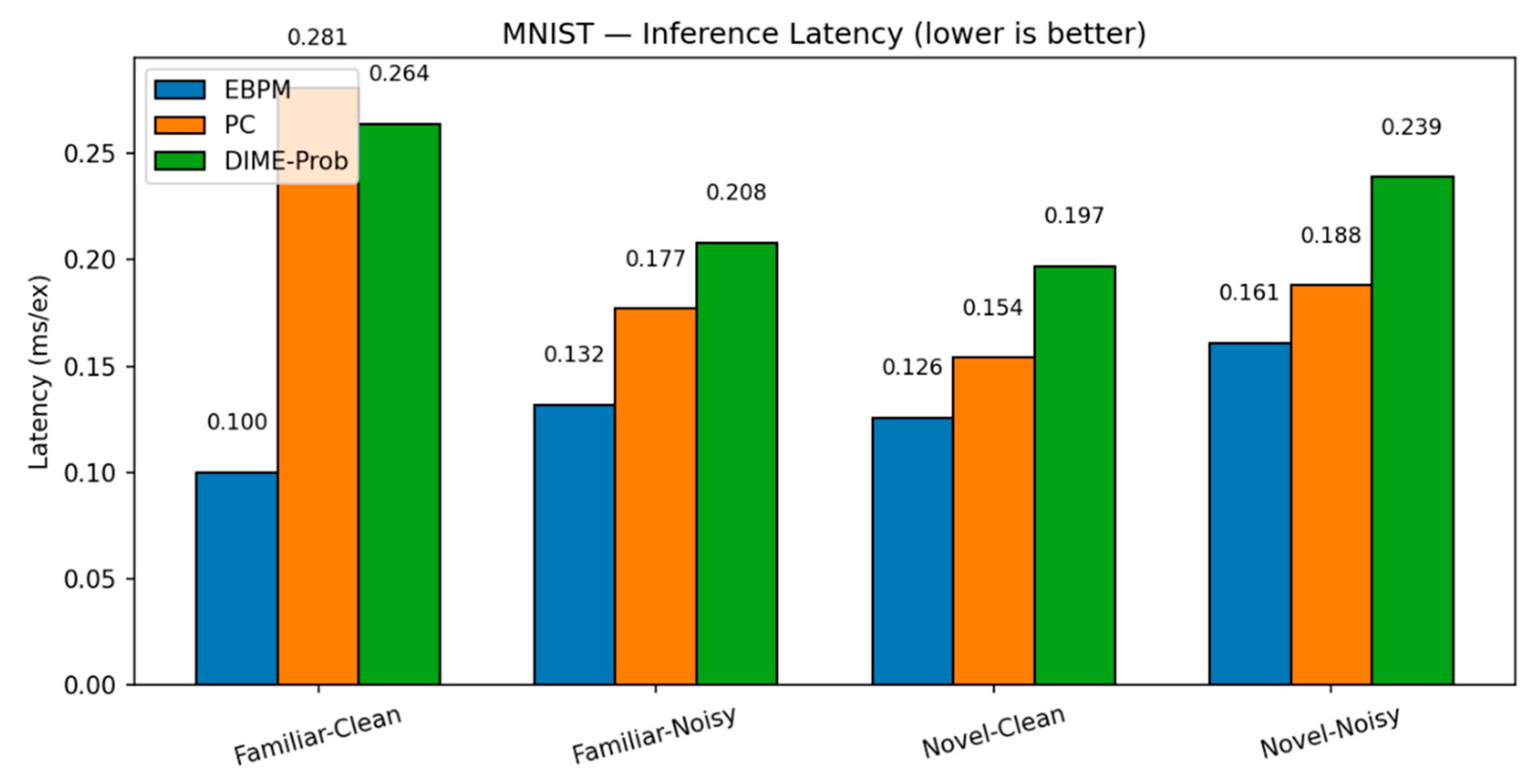
Figure 6.
MNIST: Accuracy. Top-1 accuracy on MNIST for the same four scenarios. EBPM excels on familiar but fails by design on novel (8–9); PC generalizes better to novelty; DIME balances both.
Figure 6.
MNIST: Accuracy. Top-1 accuracy on MNIST for the same four scenarios. EBPM excels on familiar but fails by design on novel (8–9); PC generalizes better to novelty; DIME balances both.
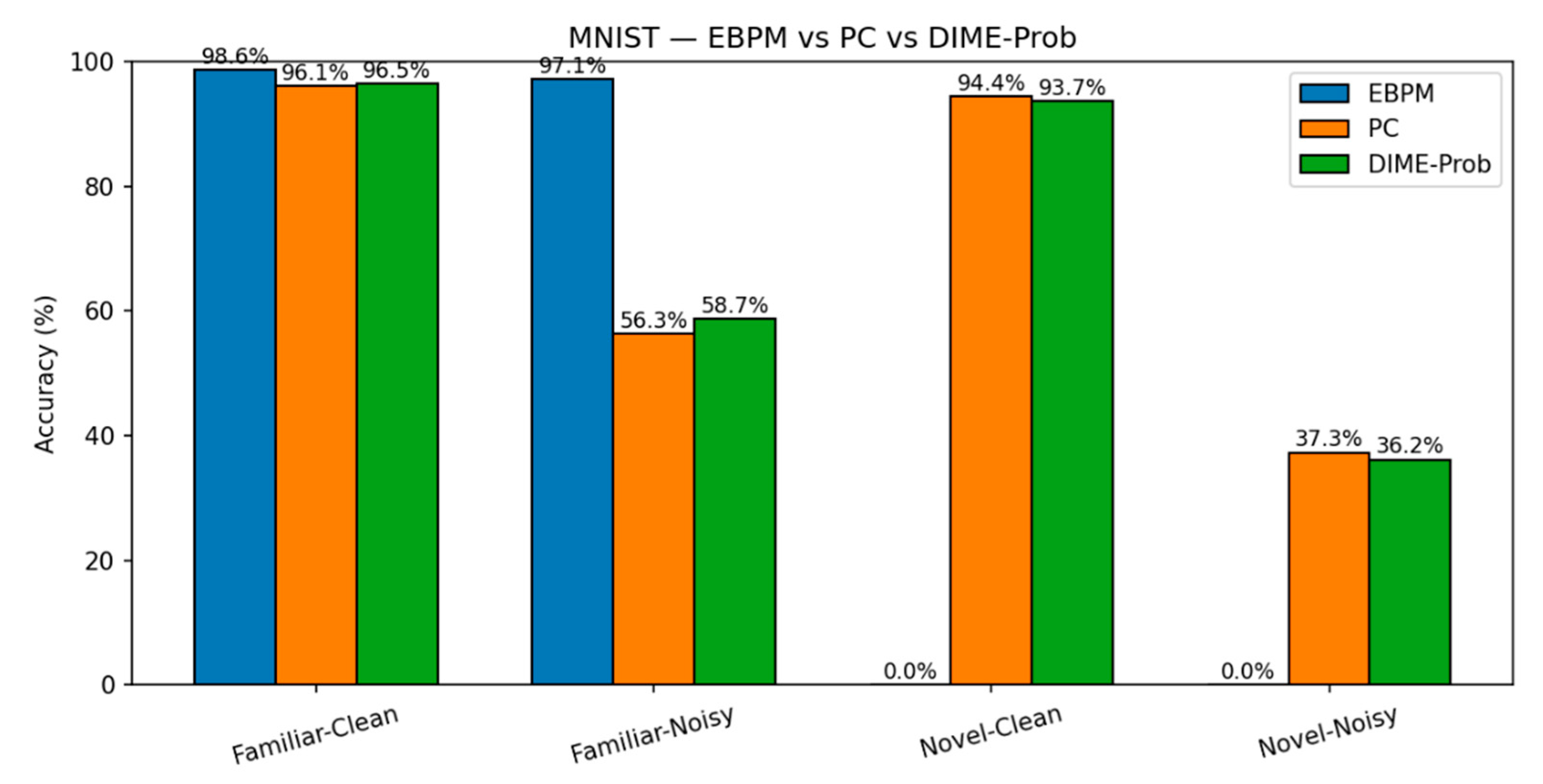
Figure 7.
Fashion-MNIST: Latency. Per-scenario latency (ms/ex.) on Fashion-MNIST for EBPM, PC (K=10, η=0.1) and DIME. Relative ordering mirrors MNIST; PC is slower due to iterative inference.
Figure 7.
Fashion-MNIST: Latency. Per-scenario latency (ms/ex.) on Fashion-MNIST for EBPM, PC (K=10, η=0.1) and DIME. Relative ordering mirrors MNIST; PC is slower due to iterative inference.
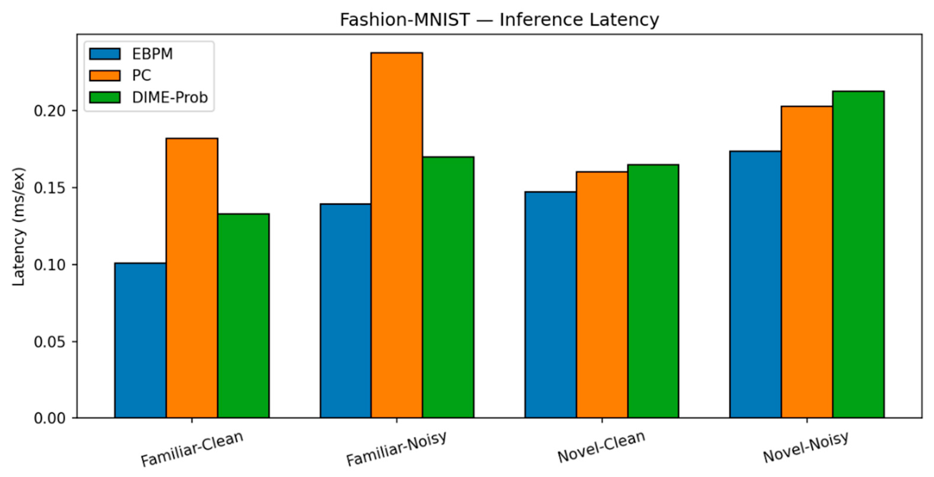
Figure 8.
Fashion-MNIST: Accuracy. Top-1 accuracy on Fashion-MNIST across the four scenarios. PC dominates on novel; EBPM is stronger on familiar; DIME interpolates context-dependently.
Figure 8.
Fashion-MNIST: Accuracy. Top-1 accuracy on Fashion-MNIST across the four scenarios. PC dominates on novel; EBPM is stronger on familiar; DIME interpolates context-dependently.
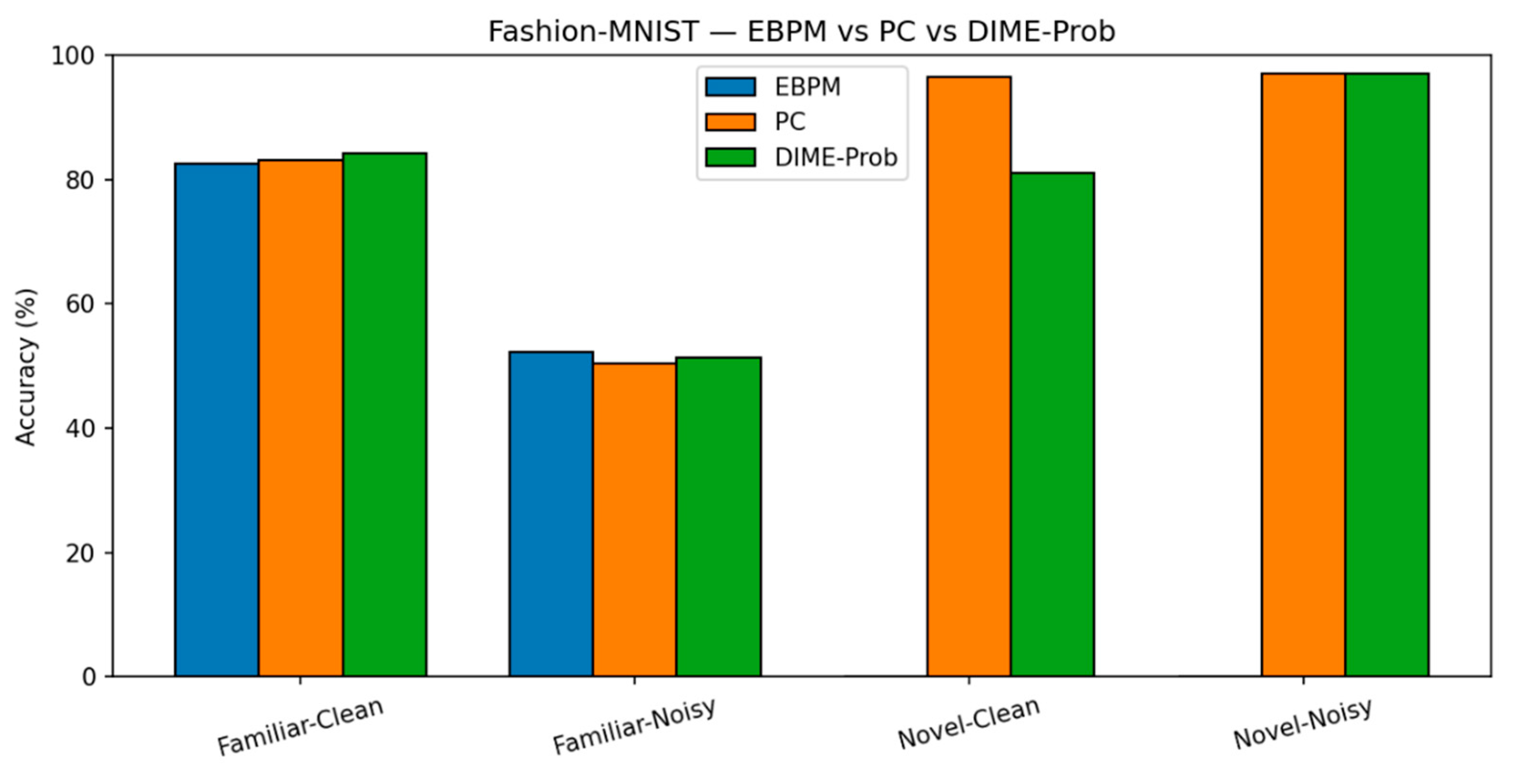
Figure 9.
CIFAR-10: Latency. Per-scenario latency on CIFAR-10. Absolute times are higher than MNIST/F-MNIST; the relative ordering EBPM < DIME ≈ PC persists.
Figure 9.
CIFAR-10: Latency. Per-scenario latency on CIFAR-10. Absolute times are higher than MNIST/F-MNIST; the relative ordering EBPM < DIME ≈ PC persists.
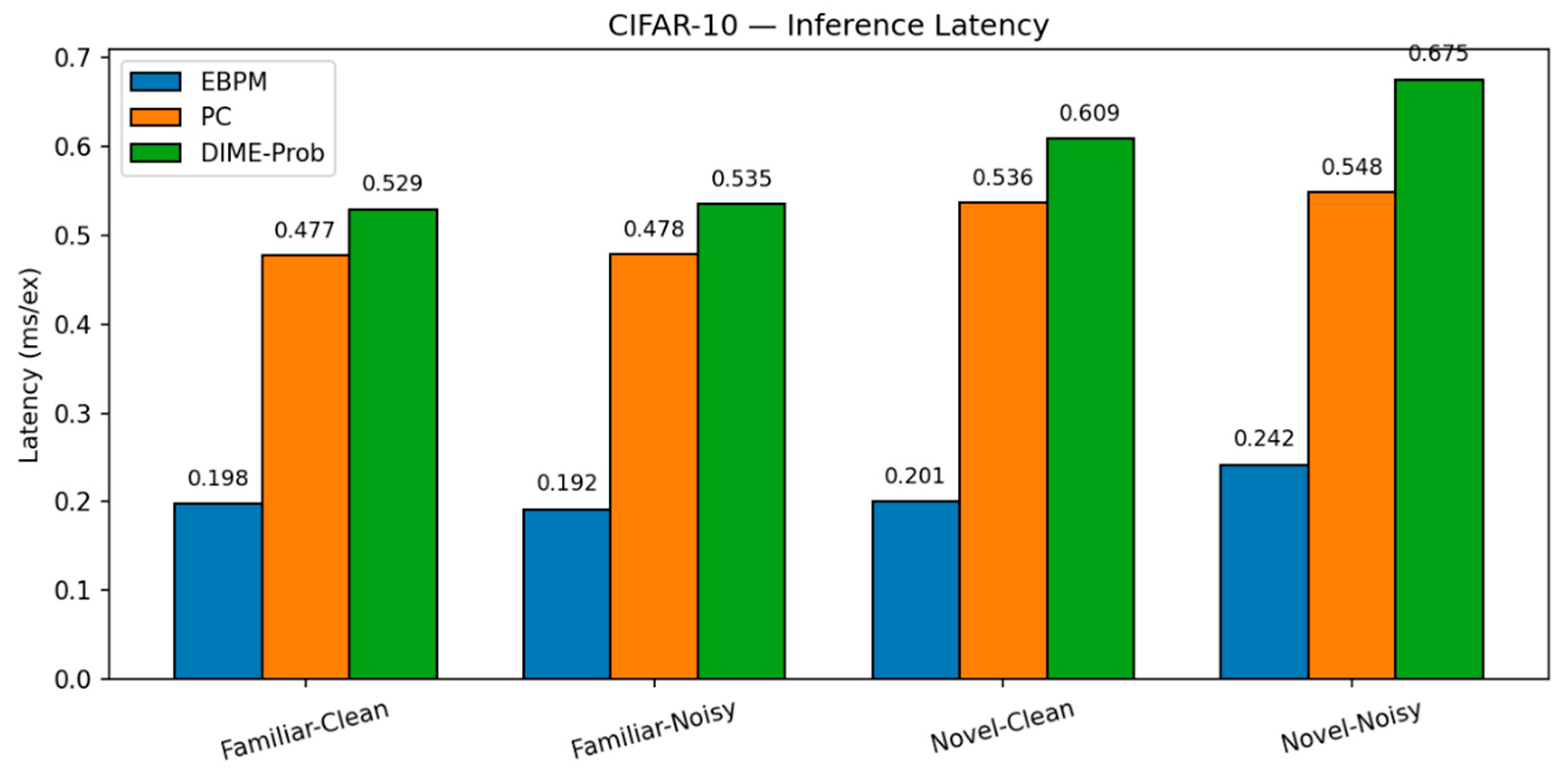
Figure 10.
CIFAR-10: Accuracy. Top-1 accuracy on CIFAR-10 for the four scenarios. PC leads on novel; EBPM degrades on noise/novel; tuned DIME-Prob trades off between the two.
Figure 10.
CIFAR-10: Accuracy. Top-1 accuracy on CIFAR-10 for the four scenarios. PC leads on novel; EBPM degrades on noise/novel; tuned DIME-Prob trades off between the two.
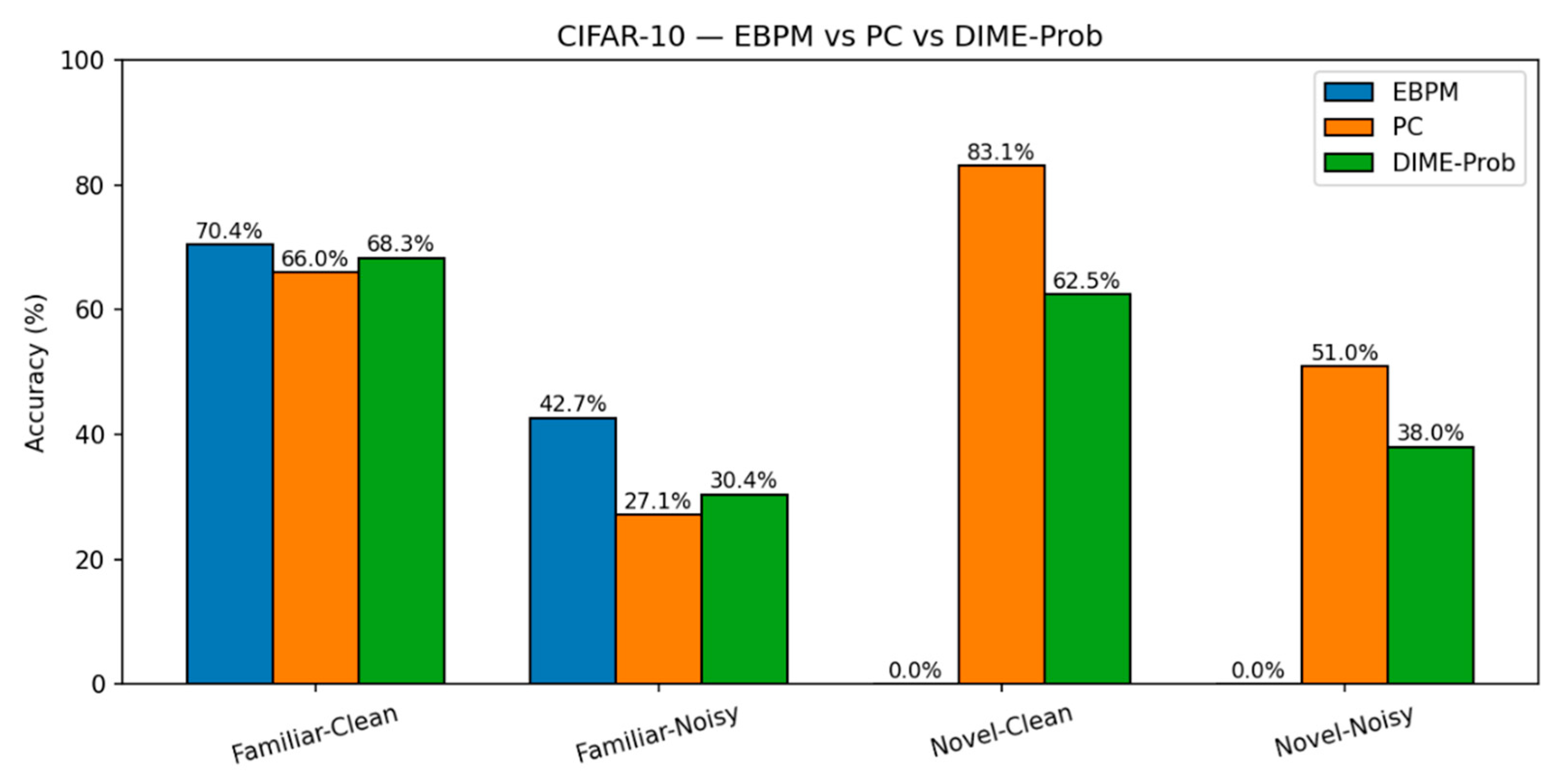
Figure 11.
MNIST: Fusion ablation. Ablation of fusion strategies: probability- vs. logit-level, familiarity calibration on/off, and iterations K. Probability-level fusion with calibration yields the best familiar/novel trade-off at comparable latency.
Figure 11.
MNIST: Fusion ablation. Ablation of fusion strategies: probability- vs. logit-level, familiarity calibration on/off, and iterations K. Probability-level fusion with calibration yields the best familiar/novel trade-off at comparable latency.
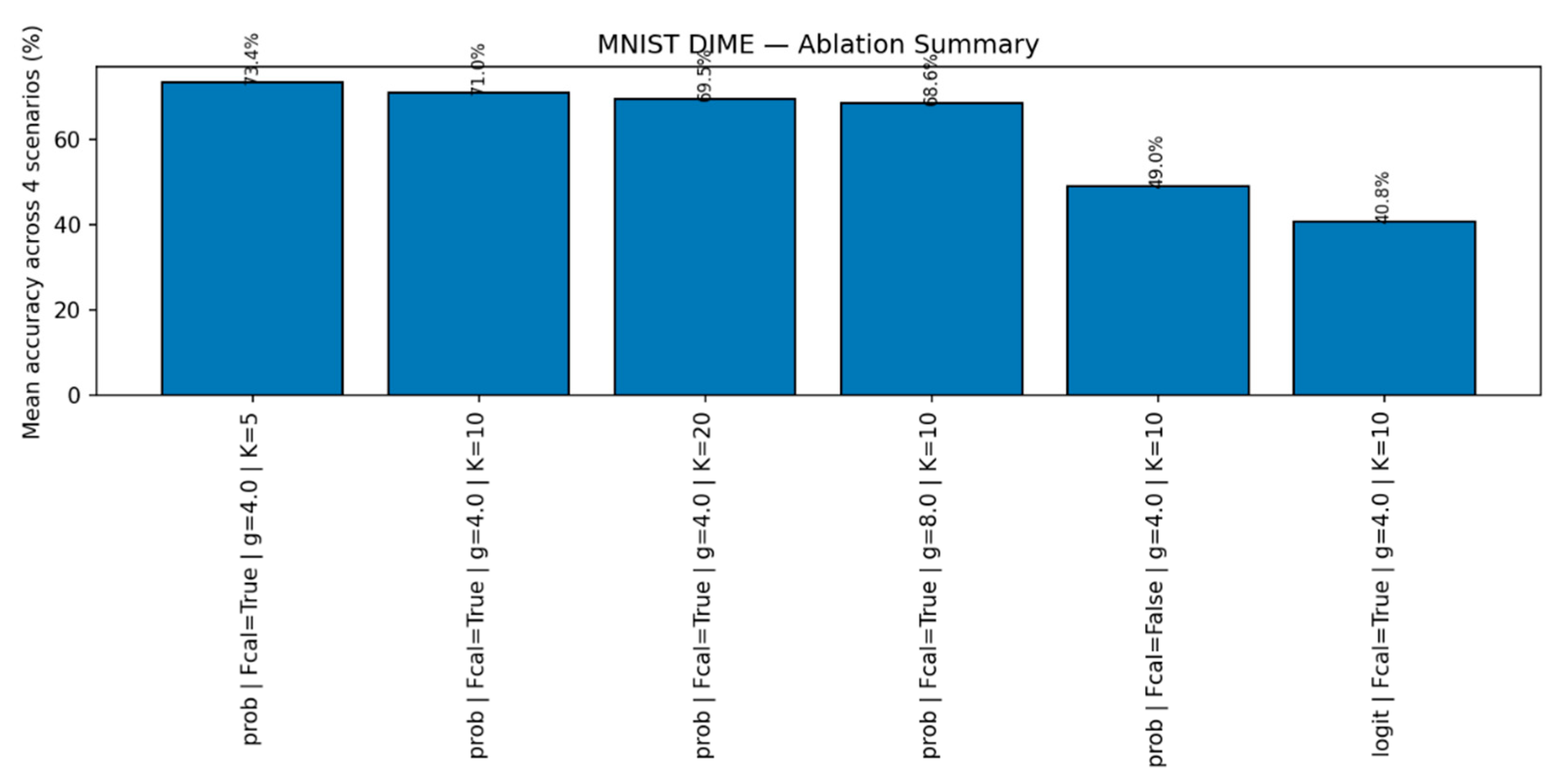
Figure 12.
MNIST: Mean α. Mean fusion weight ᾱ per scenario showing how DIME shifts between EBPM and PC as uncertainty changes.
Figure 12.
MNIST: Mean α. Mean fusion weight ᾱ per scenario showing how DIME shifts between EBPM and PC as uncertainty changes.
3.2. Comparative Results and Simulations
To evaluate the potential of the DIME model, we conducted a comparison across five critical dimensions: speed, energy efficiency, robustness to noise, flexibility, and biological plausibility.
- EBPM: performs well in speed and efficiency, but is limited in adaptation and robustness.
- PC: flexible and robust, but entails high costs.
- DIME: integrates the advantages of both, providing an optimal balance between speed, efficiency, and flexibility.
For a conceptual comparison, see Appendix Figure C1; the main text reports only empirical results.
3.3. General Information Flow in DIME
DIME organizes perception along two complementary paths (Figure 13): (1) a fast EBPM path that maps inputs to a normalized embedding and matches against class prototypes, and (2) a slower PC path that iteratively refines a latent code to improve reconstruction and classification. A controller α∈[0,1] balances the two outputs at inference time—favoring EBPM in familiar, low-noise settings and shifting toward PC as uncertainty or novelty increases. This flow underlies the empirical trade-offs reported in §3.1 and the runtime behavior in §3.4. [29], [25].
3.4. Virtual Robotics (Obstacle Course): Runtime-Aware DIME-Lazy (α Fixed)
Figure 14.
Obstacle course (snapshot). Top-down orthographic view of the obstacle course. R = robot, T = target, O1–O4 = obstacles; frames from this camera are down-sampled to 28×28 grayscale.
Figure 14.
Obstacle course (snapshot). Top-down orthographic view of the obstacle course. R = robot, T = target, O1–O4 = obstacles; frames from this camera are down-sampled to 28×28 grayscale.
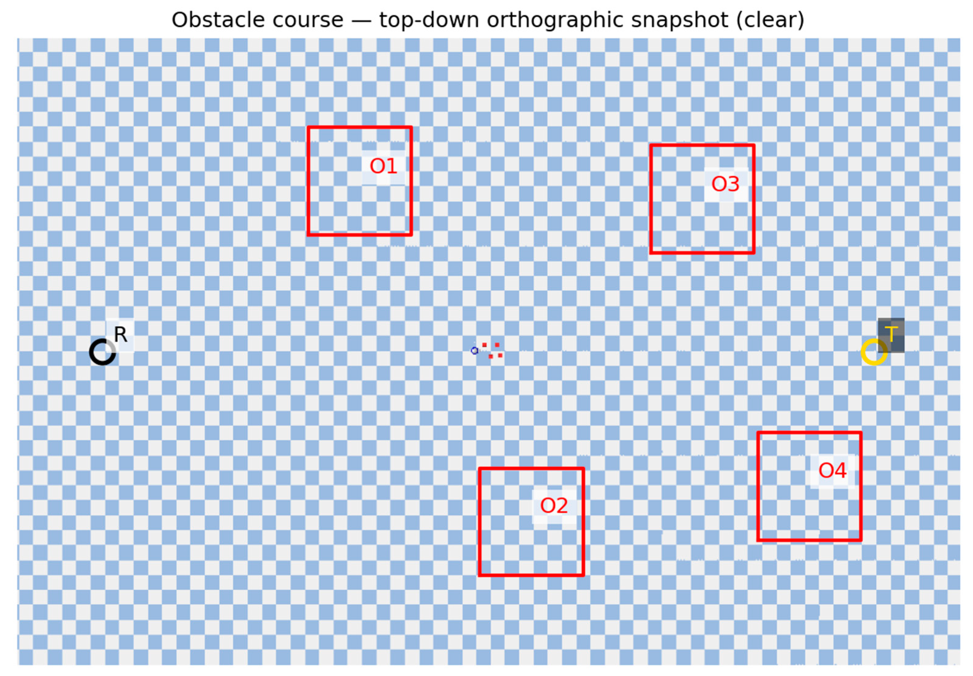
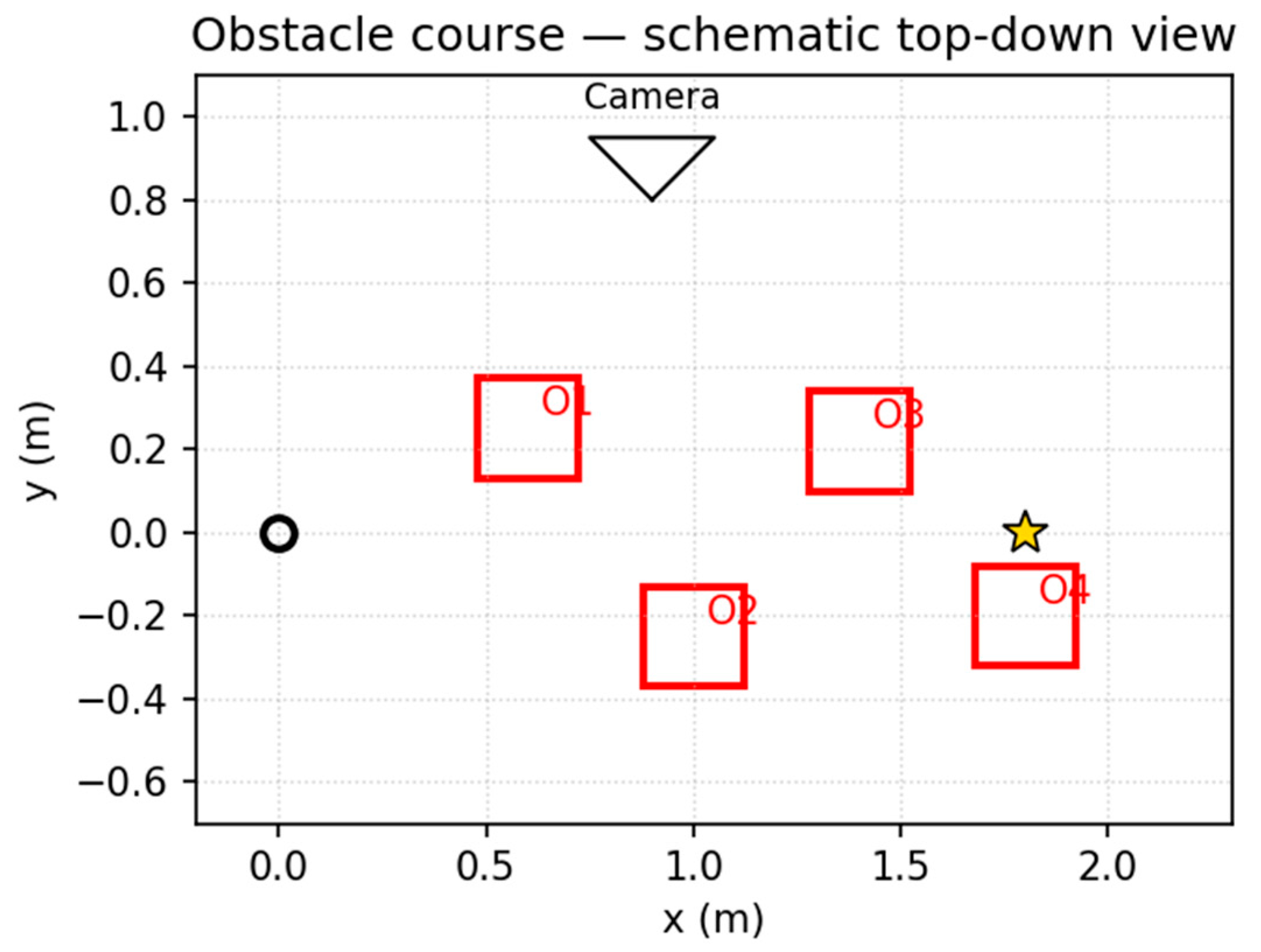
Figure 15.
Obstacle course (schematic). Clean 2D schematic with waypoints used by the kinematic velocity controller (v_max=1.2 m/s, WP_RADIUS=0.55 m).
Figure 15.
Obstacle course (schematic). Clean 2D schematic with waypoints used by the kinematic velocity controller (v_max=1.2 m/s, WP_RADIUS=0.55 m).
We evaluated EBPM, PC, DIME and a runtime-aware variant, DIME-Lazy, in a PyBullet obstacle-course with four static boxes and an overhead camera. The controller was kinematic (velocity) following a fixed waypoint slalom; thus, task success is identical across methods and any runtime differences isolate perception cost. The camera frames were down-sampled to 28×28 grayscale. DIME-Lazy uses a delta-frame gate: for each step we compute δ = mean(|It − It−1|). If δ ≤ 0.004 ⇒ EBPM-only; if δ ≥ 0.015 ⇒ PC-only; otherwise we fuse with a fixed α = 0.65: p = α p_EBPM + (1 − α) p_PC.
Waypoints: (0.45, 0.45) → (0.85, −0.45) → (1.25, 0.40) → (1.60, −0.30) → (1.80, 0.00); controller v_max=1.2 m/s; WP_RADIUS = 0.55 m. Each condition ran for 3 episodes. Metrics: ms/step, success rate, collisions (contact frames), and #PC calls.
Key findings. With noise=0.0, DIME-Lazy matches EBPM’s decisions (0 PC calls) and achieves the lowest cost (10.50 ms/step), ~−42% vs. PC (18.04 ms) and ~−32% vs. EBPM (15.43 ms), at 100% success. With noise=0.15, DIME-Lazy escalates toward PC (≈380 PC calls/381) and its cost matches PC (19.17 vs. 19.13 ms), again at 100% success. Collisions are equal across methods (mean 113), confirming runtime comparisons are not confounded by control (see Figure 16 and Figure 17).
Table 6.
PyBullet obstacle course — means over 3 episodes (v3c_alpha, α=0.65).
| mode | noise | ms/step (mean) |
steps (mean) |
success | collisions (mean) |
|---|---|---|---|---|---|
| EBPM | 0.00 | 15.43 | 381 | 1.00 | 113 |
| PC | 0.00 | 18.04 | 381 | 1.00 | 113 |
| DIME | 0.00 | 18.44 | 381 | 1.00 | 113 |
| DIME-Lazy | 0.00 | 10.50 | 381 | 1.00 | 113 |
| EBPM | 0.15 | 12.55 | 381 | 1.00 | 113 |
| PC | 0.15 | 19.13 | 381 | 1.00 | 113 |
| DIME | 0.15 | 19.52 | 381 | 1.00 | 113 |
| DIME-Lazy | 0.15 | 19.17 | 381 | 1.00 | 113 |
4. Discussion
4.1. Advantages of EBPM
The EBPM model explains the rapid and energy-efficient reactions observed in familiar contexts. In contrast to PC, where the cortex must continuously generate internal predictions [2], EBPM assumes that a sensory stimulus directly activates the relevant engram. This mechanism reduces latencies and energy cost, in agreement with neurophysiological data showing that neuronal assemblies reactivate almost instantaneously when familiar stimuli are encountered [4].
Another advantage lies in procedural robustness. Complex but overlearned actions—such as the use of a tool—can be initiated through the direct reactivation of a multimodal engram, without the need for predictive simulations. This aspect correlates with the observations of Hawkins and Ahmad [5], who showed that neurons possess thousands of synapses precisely to facilitate the rapid reactivation of memorized sequences.
The §2.3.6 comparison shows EBPM covers familiar inputs with minimal compute, while generative or external-memory approaches excel on novelty; DIME reconciles the two.
Nevertheless, EBPM recognition is contingent on the prior existence of well-consolidated engrams. In situations where no such engrams are available, EBPM cannot operate effectively, which limits its explanatory power in novel or ambiguous contexts.
4.2. Limitations of EBPM
A frequently raised concern is that EBPM, by design, yields near-zero accuracy on entirely novel inputs. However, this should not be interpreted as a failure but rather as a functional distinction: EBPM explicitly separates the processes of recognition and novelty detection.
In EBPM, unfamiliar stimuli still activate sub-engrams (elementary sensory, motor, or interoceptive primitives). Although none of the stored engrams reach full activation, the fragmentary sub-engram activity defines a novelty state. This state automatically triggers attentional mechanisms that increase neuronal gain and plasticity, promoting the binding of co-active sub-engrams into a proto-engram. With repetition or behavioral relevance, this proto-engram consolidates into a stable engram; without reinforcement, the weak associations fade [30].
Thus, the “0% accuracy” in novel conditions is not a bug but an intentional feature: EBPM does not force a misclassification under uncertainty. Instead, it signals novelty and reallocates resources toward exploration and learning. From a biological standpoint, this aligns with evidence that attention and neuromodulatory systems (e.g., locus coeruleus–noradrenaline) are engaged precisely when established assemblies fail to reactivate. From an engineering perspective, this provides an explicit novelty-flagging mechanism that can be exploited in hybrid systems such as DIME, where PC takes over under unfamiliar or noisy conditions.
In summary, EBPM’s limitation is also its defining contribution: while it cannot generalize to novel inputs on its own, it provides a biologically grounded mechanism for rapid recognition of the familiar and explicit detection of the unfamiliar, thereby laying the groundwork for adaptive integration with generative models.
4.3. Advantages of PC
Predictive Coding (PC) compensates for these limitations through its flexibility and robustness. Because the cortex generates top–down predictions, it can reconstruct incomplete or noisy inputs. This explains, for example, why we are able to recognize an object even when it is partially occluded [31]. Moreover, PC is supported by strong neuroimaging evidence demonstrating the active presence of anticipatory signals in higher-order cortical areas [32].
Importantly, PC also remains valuable for explaining how new engrams can be formed under conditions of partial or conflicting input. Its recursive comparison mechanism provides a plausible account of how the brain integrates incomplete information and adapts to unforeseen circumstances.
4.4. Limitations of PC
However, PC entails a high energetic cost and longer latencies. The continuous process of generating and verifying predictions is inefficient in familiar situations, where direct recognition would be sufficient. This observation is consistent with the arguments put forward by Kanai et al. [3], who highlighted that maintaining a complete generative model is redundant in stable and well-known contexts.
A more fundamental critique of PC concerns the very notion of “prediction” as an active top–down mechanism. From a neurobiological perspective, there is no evidence for explicit reconstructions of sensory input at lower levels. What actually exists are engrams, i.e., networks consolidated through experience and synaptic plasticity, according to the principle “neurons that fire together wire together”. When incoming stimuli sufficiently reactivate these networks (for example, edges + red color + cylindrical shape → cup), recognition arises directly from this reactivation. There is no top–down “drawing” of the cup into the visual cortex; there are only pre-trained networks that fire automatically when the input matches. If, however, the object is missing, chipped, or altered (e.g., covered with flour), the activation of the engram is partial or inconsistent, which triggers attention, learning, and the formation of new connections. In this interpretation, the top–down flow does not generate explicit predictions, but functions as a modulation of excitability in lower-level networks, sensitizing them according to context and goals.
This role of top–down signaling becomes particularly evident in imagination and internal simulation. When a person “falls into thought” or mentally visualizes an object, associative and hippocampal networks reactivate engrames and transmit activity top–down to sensory cortices, so that one can “see” the cup or “hear” a melody in the mind without any external input. In parallel, there is an active inhibition of real sensory inputs, which explains why people become less attentive to the environment during deep thought. Everyday examples confirm this inhibitory control: when an ophthalmologist blows air into the eye but the voluntary system suppresses the blink reflex; or when a nurse administers an injection and, despite the painful stimulus, the prefrontal cortex modulates motor pathways to block the withdrawal reflex. Similar effects are seen when athletes suppress avoidance reflexes to perform risky movements, or when musicians ignore sudden noises to remain focused. These examples illustrate that top–down influence is primarily about gain control and inhibition, not about generating full sensory predictions.
Moreover, PC also fails to account for fast reflexes and highly automated responses, which bypass any generative comparison process. Reflexes such as blinking to corneal stimulation or withdrawing from a painful stimulus are executed through subcortical or spinal circuits within tens of milliseconds, long before any top–down “prediction” could be generated or verified. Similarly, well-learned sensorimotor routines (e.g., skilled grasping or locomotion patterns) unfold primarily through engram reactivation in cortico-basal ganglia and cerebellar loops, with minimal involvement of predictive feedback. This further highlights that PC cannot serve as a universal principle of recognition and behavior, but at most as an auxiliary attentional mechanism in situations of novelty, conflict, or noise.
Taken together, these considerations suggest that PC is not the primary engine of recognition but rather a set of attentional and executive sub-mechanisms. EBPM provides a more direct explanation for rapid and low-cost recognition through engram reactivation, while PC becomes relevant mainly when engram activation is insufficient, inconsistent, or requires inhibition of automatic responses.
A further limitation of PC lies in the absence of a clear neurobiological specification of how predictions are generated. In most formulations, the “prediction” is treated as an abstract top–down signal, with little explanation of the concrete neuronal mechanisms that produce it. Empirical evidence suggests that top–down pathways modulate the excitability of lower-level networks rather than reconstructing full sensory input, leaving the precise nature of the predictive signal underspecified. In contrast, EBPM explicitly defines recognition as the reactivation of consolidated engrams, including the conditions under which activation is complete, partial, or inconsistent, and how attention and learning intervene in the latter cases. Within the DIME framework, this provides a mechanistic clarity absent from PC, while still allowing PC-like processes to be reinterpreted as attentional subroutines engaged in novelty and ambiguity.
4.5. Threats to Validity and Limitations
Internal validity. Our familiar/novel split (0–7 vs. 8–9) is standard but creates a sharp novelty boundary; different splits could change absolute numbers. Familiarity calibration (μ,σ) for DIME was estimated on familiar validation images; miscalibration would shift α and the EBPM↔PC balance.
Construct validity. Accuracy and ms/step capture complementary aspects (task performance vs. compute cost), but do not measure uncertainty calibration or open-set risk explicitly.
External validity. CIFAR-10 and MNIST/F-MNIST are limited in complexity; generalization to natural, long-tail distributions requires larger models/datasets. The PyBullet course uses a fixed waypoint controller; success equality across methods isolates perception cost but does not evaluate closed-loop policy learning.
Conclusion validity. Some robotics metrics average over 3 episodes; while stable, they may under-estimate rare failure modes. We therefore report means and provide raw CSV files for replication.
Future work. We will evaluate on stronger open-set/OOD benchmarks, vary the novelty boundary, increase episode counts, and explore learned gating for DIME-Lazy beyond fixed α and thresholds.
Appendix captions: Figure E1–E2 — Hypothesized trends (non-empirical). Hypothetical plots used during design; retained for transparency. Not used to support claims.
Parallels with the Predictive Coding trajectory. It is important to emphasize that the EBPM/DIME framework should be understood as a theoretical synthesis, not as an isolated speculation. Its components—engram reactivation, Hebbian/STDP plasticity, lateral inhibition, attentional gain, and LC–NE novelty signaling—are all individually supported by empirical evidence in both animal and human studies. The novelty of EBPM lies in integrating these mechanisms into a unified account of recognition and novelty detection. In this respect, EBPM’s current status is comparable to that of Predictive Coding (PC) at the time of its initial formulation: PC was accepted as a dominant paradigm long before all of its assumptions were empirically confirmed, and to this day some of its central claims (e.g., explicit generative reconstructions in primary cortices, “negative spike” signals) remain debated. EBPM/DIME thus follows a similar trajectory: built on solid empirical fragments, it provides a coherent alternative framework whose integrative claims now require systematic validation through the experimental program outlined in §2.5.
4.6. DIME as an Integrative Solution
Given these complementary characteristics, the proposed model—DIME (Dynamic Integrative Matching and Encoding)—offers a balanced solution. By combining the two paradigms, DIME enables both rapid recognition through EBPM in familiar situations and generative inference through PC in ambiguous conditions. The dynamic controller determines the dominant pathway depending on the level of familiarity and uncertainty. This type of architecture reflects the recent view of the brain as a hybrid system that combines fast associations with slower but more flexible inferences. [19].
To evaluate the advantages and limitations of each model, we synthesized the main characteristics in Table 7. This comparison shows that EBPM achieves peak performance in speed and energy efficiency but is less adaptable. PC excels in flexibility and noise robustness, yet entails higher computational and energetic costs. DIME successfully integrates the advantages of both paradigms, offering a better balance between performance, adaptability, and biological plausibility. This suggests that such integration not only reflects the functioning of the brain more faithfully but also provides a promising direction for the design of efficient AI and robotic systems.
A comparative table-style figure or infographic:
- EBPM = fast, energy-efficient, but less flexible.
- PC = robust, adaptive, but computationally costly.
- DIME = hybrid integration, balancing both.
Table 7 summarizes strengths and limitations of EBPM, PC, and DIME. EBPM excels in speed and energy efficiency, PC in flexibility and noise robustness, and DIME provides an integrative balance. Such comparative tables are common in neurocomputational model reviews [20,33].
The ANN results (Table 5a-5c, Figure 5, Figure 6, Figure 7, Figure 8, Figure 9, Figure 10 and Figure 11) empirically validate these claims: EBPM excels in speed and efficiency, PC in robustness, and DIME dynamically balances both. The α controller consistently shifted toward EBPM on familiar inputs and toward PC under noise and novelty, in agreement with the theoretical model.
4.7. Interdisciplinary Implications
- Neuroscience: EBPM provides an alternative explanation for the phenomenon of memory replay, while DIME may serve as a more faithful framework for understanding the interaction between memory and prediction.
- Artificial Intelligence: EBPM-inspired architectures are more energy-efficient, and their integration with PC-type modules can enhance noise robustness.
In artificial intelligence, EBPM also resonates with memory-augmented neural architectures such as Neural Turing Machines [15], Differentiable Neural Computers [16], and episodic control models in reinforcement learning [17]. Unlike these approaches, which are primarily engineered solutions, EBPM emphasizes biological grounding through multimodal engram reactivation. DIME can therefore be interpreted as a bridge between biologically plausible engram-based recall and machine-oriented predictive architectures.
5. Conclusions
This paper has introduced and compared two fundamental paradigms of neural processing: Predictive Coding (PC), an established framework in neuroscience [1,2], and the original Experience-Based Pattern Matching (EBPM) model, proposed here for the first time. The comparative analysis highlighted that EBPM provides clear advantages in familiar contexts: faster recognition, increased energy efficiency, and better consistency with phenomena of direct memory reactivation (multimodal engrams)[4,30]. In contrast, PC remains superior in ambiguous situations or with incomplete inputs, due to its anticipatory reconstruction capability [31].
Nevertheless, neither of the two models fully accounts for all observed cognitive phenomena. For this reason, we proposed a new integrative framework—DIME (Dynamic Integrative Matching and Encoding)—which combines EBPM’s direct matching with PC’s generative prediction. DIME incorporates a dynamic controller that determines the dominant processing pathway depending on familiarity, uncertainty, and goals. Theoretical results and preliminary simulations suggest that DIME provides an optimal balance between speed, efficiency, and robustness, making it both more biologically plausible and more practically useful than the individual models.
This contribution has interdisciplinary implications:
- in neuroscience, it provides a more comprehensive explanation of the interaction between memory and prediction,
- in artificial intelligence, it suggests hybrid architectures that are more energy-efficient,
- in robotics, it paves the way for autonomous systems that can combine rapid recognition with adaptability to unfamiliar environments.
The present ANN simulations provide the first concrete validation of the DIME model, supporting its potential for integration into both neuroscience frameworks and robotic control architectures.
In the future, validating the DIME model will require: (i) high-resolution neuroimaging experiments to test the dynamics of engram activation versus prediction, (ii) large-scale ANN simulations to evaluate scalability, and (iii) robotic implementations to quantify the advantages in real environments.
In conclusion, EBPM represents an original contribution to cognitive modeling, while DIME provides a hybrid framework with the potential to redefine how we interpret neural computation and apply it in intelligent systems.
Data & Code Availability
All scripts, configuration files, and raw outputs for ANN (MNIST, Fashion-MNIST, CIFAR-10) and PyBullet experiments are provided as a supplementary package and anonymized ZIP provided to reviewers; public links added after acceptance. The figures in the main text correspond to image files listed in MANIFEST.md under Supplementary/figures/, and the raw numeric results are provided as CSV/TXT under Supplementary/results_csv/ and Supplementary/results_txt/. For exact reproduction we include environment versions (Python/PyTorch/CUDA), random seeds, and runnable commands in README.md. An immutable archive will be deposited on Zenodo at acceptance, and the DOI will be added to this section.
A blind, anonymous link to the supplementary ZIP is provided via the submission system; the public GitHub/Zenodo links will be added upon acceptance.
The supplementary repository includes all scripts used to produce the results (see experiments/mnist_all.py, fashion_mnist_all.py, cifar10_all.py) and a minimal robotics scaffold (robotics/pybullet_setup_demo.py), together with exact seeds, default hyper-parameters, and ready-to-run commands. Raw TXT/CSV outputs and plotting utilities are provided alongside.
Appendix A
Figure A1.
EBPM vs. PC (Latency). Latency comparison restricted to EBPM vs. PC (K=10, η=0.1).
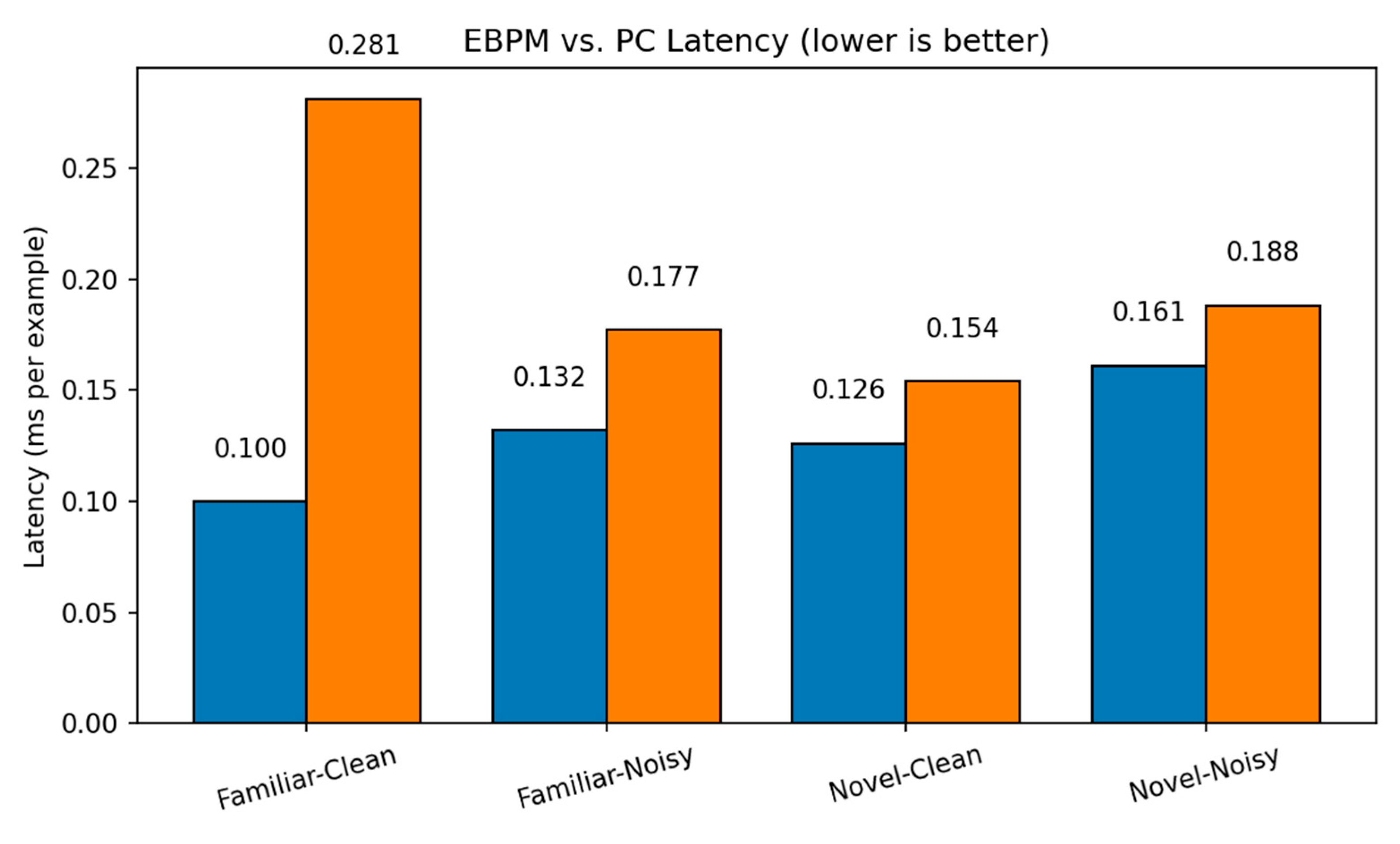
Figure A2.
EBPM vs. PC (Accuracy). Accuracy comparison restricted to EBPM vs. PC.
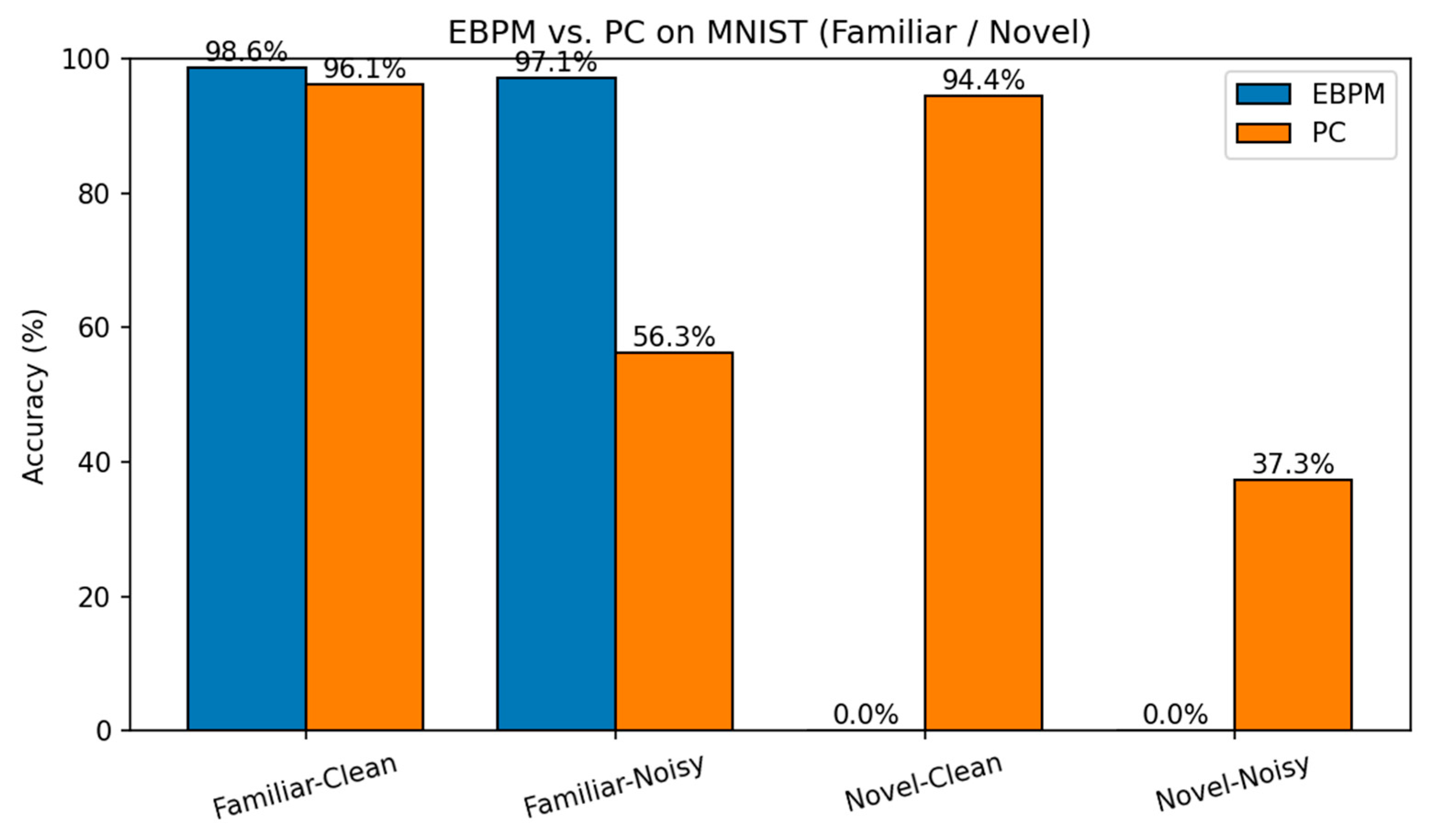
Figure R1.
Legacy ms/step bar chart. Historic bar chart of ms/step on an older configuration. Superseded by the v3c_alpha results.
Figure R1.
Legacy ms/step bar chart. Historic bar chart of ms/step on an older configuration. Superseded by the v3c_alpha results.
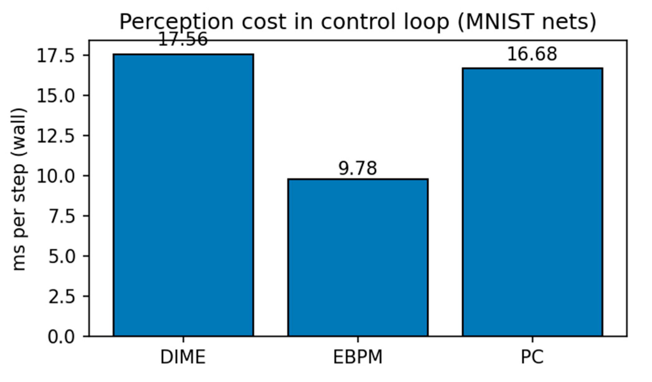
Figure R2.
Legacy DIME-Lazy ms/step. Older view of DIME-Lazy perception cost; thresholds and controller differ from the final setup.
Figure R2.
Legacy DIME-Lazy ms/step. Older view of DIME-Lazy perception cost; thresholds and controller differ from the final setup.
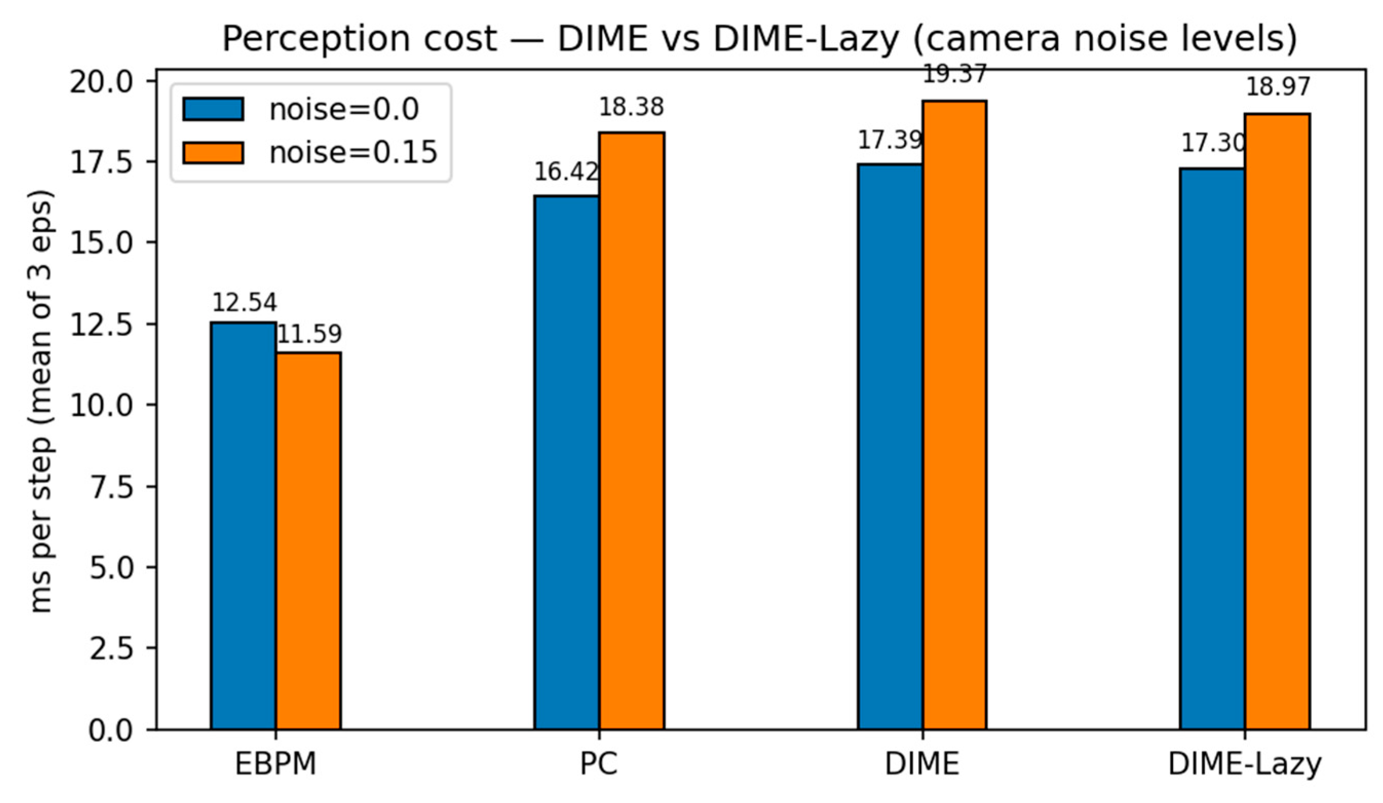
Figure R3.
Legacy obstacles ms/step. Earlier ms/step summary on the obstacle scenario. Kept as a historical reference; the main text reports v3c_alpha.
Figure R3.
Legacy obstacles ms/step. Earlier ms/step summary on the obstacle scenario. Kept as a historical reference; the main text reports v3c_alpha.
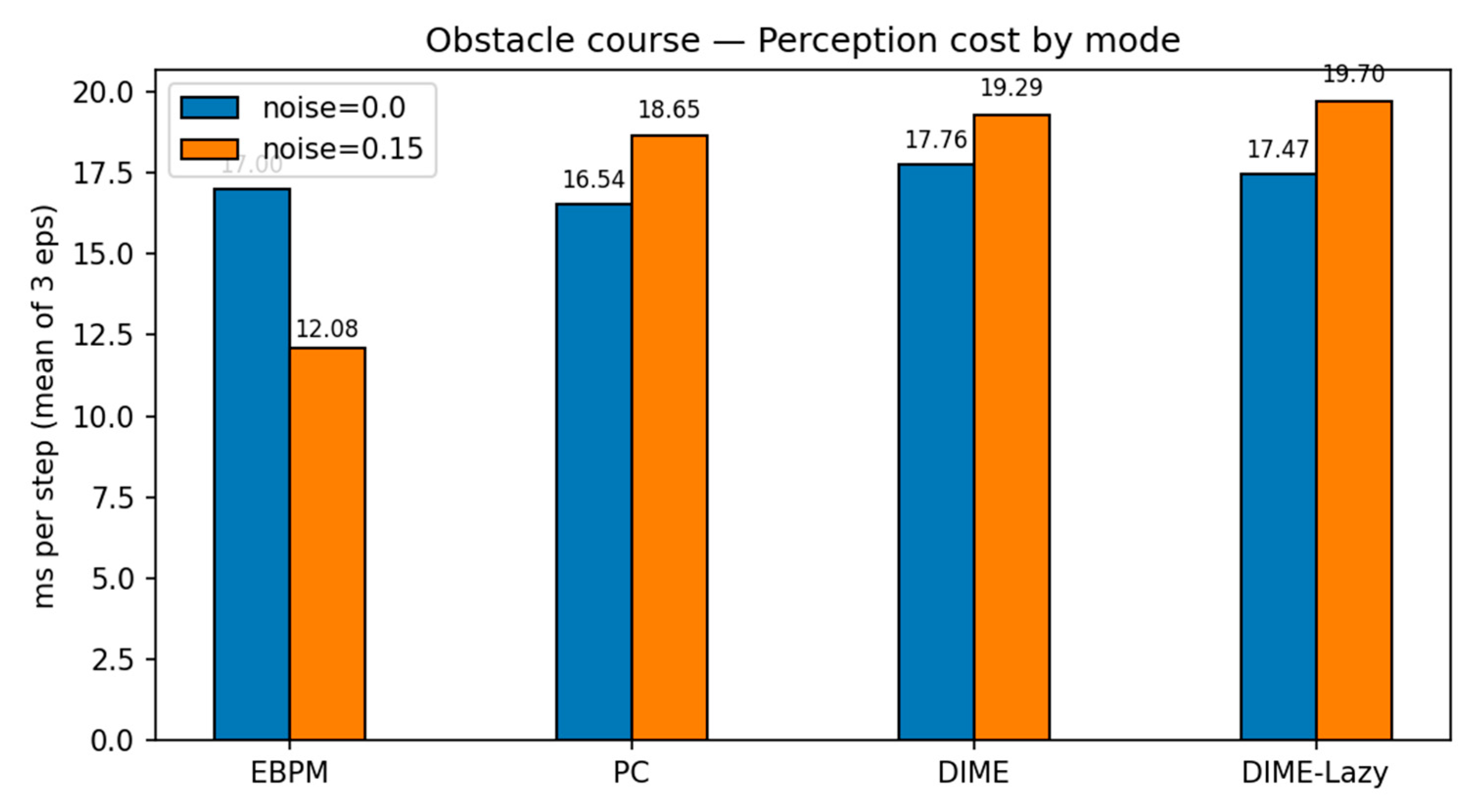
Figure C1.
Conceptual radar comparison. Conceptual (non-empirical) illustration of expected tendencies for EBPM, PC, and DIME across speed, robustness to noise/novelty, and compute cost. Provided for intuition only; not derived from measured data.
Figure C1.
Conceptual radar comparison. Conceptual (non-empirical) illustration of expected tendencies for EBPM, PC, and DIME across speed, robustness to noise/novelty, and compute cost. Provided for intuition only; not derived from measured data.
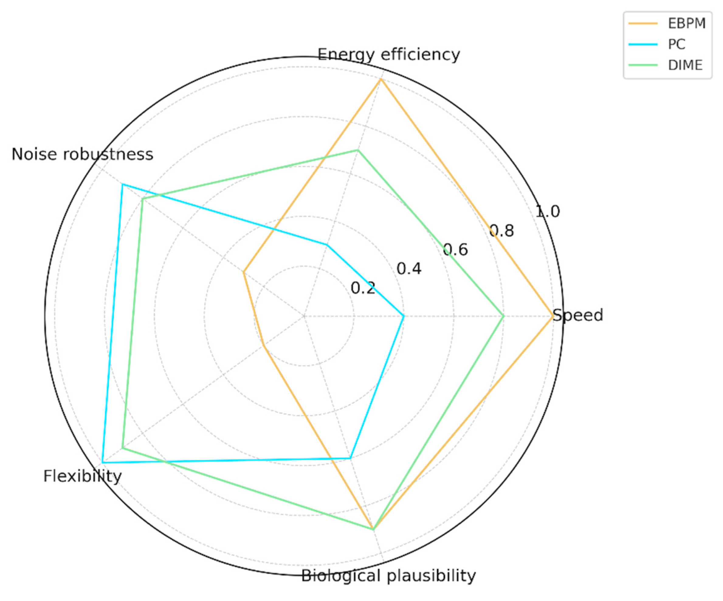
Figure E1.
a. Predicted EEG/MEG recognition latency (ms) with 95% CI: EBPM ≈ 250±40, PC ≈ 400±60.
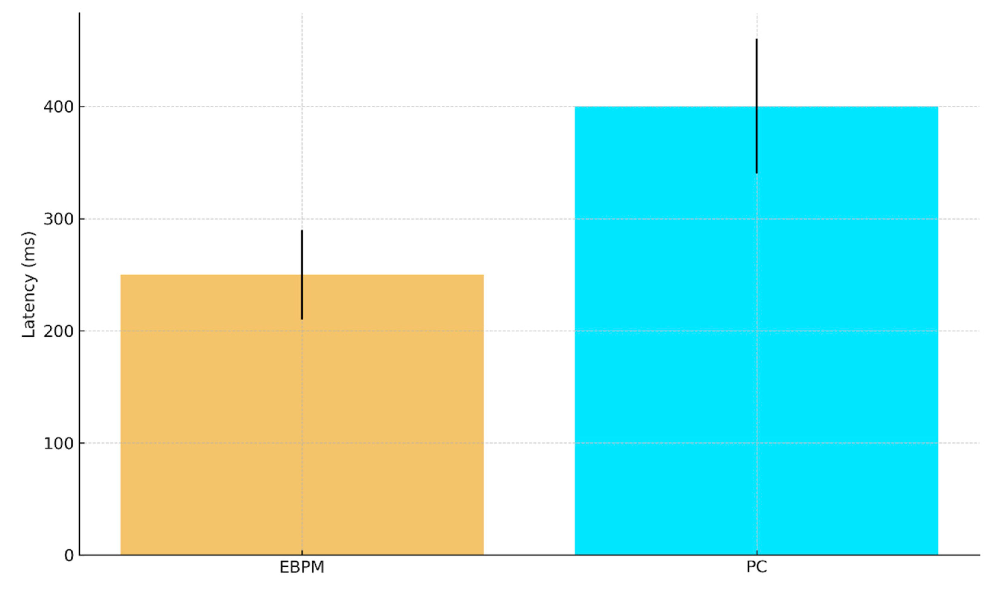
Figure E1.
b. Predicted fMRI RSA (r) with 95% CI: EBPM ≈ 0.75±0.05, PC ≈ 0.60±0.07.
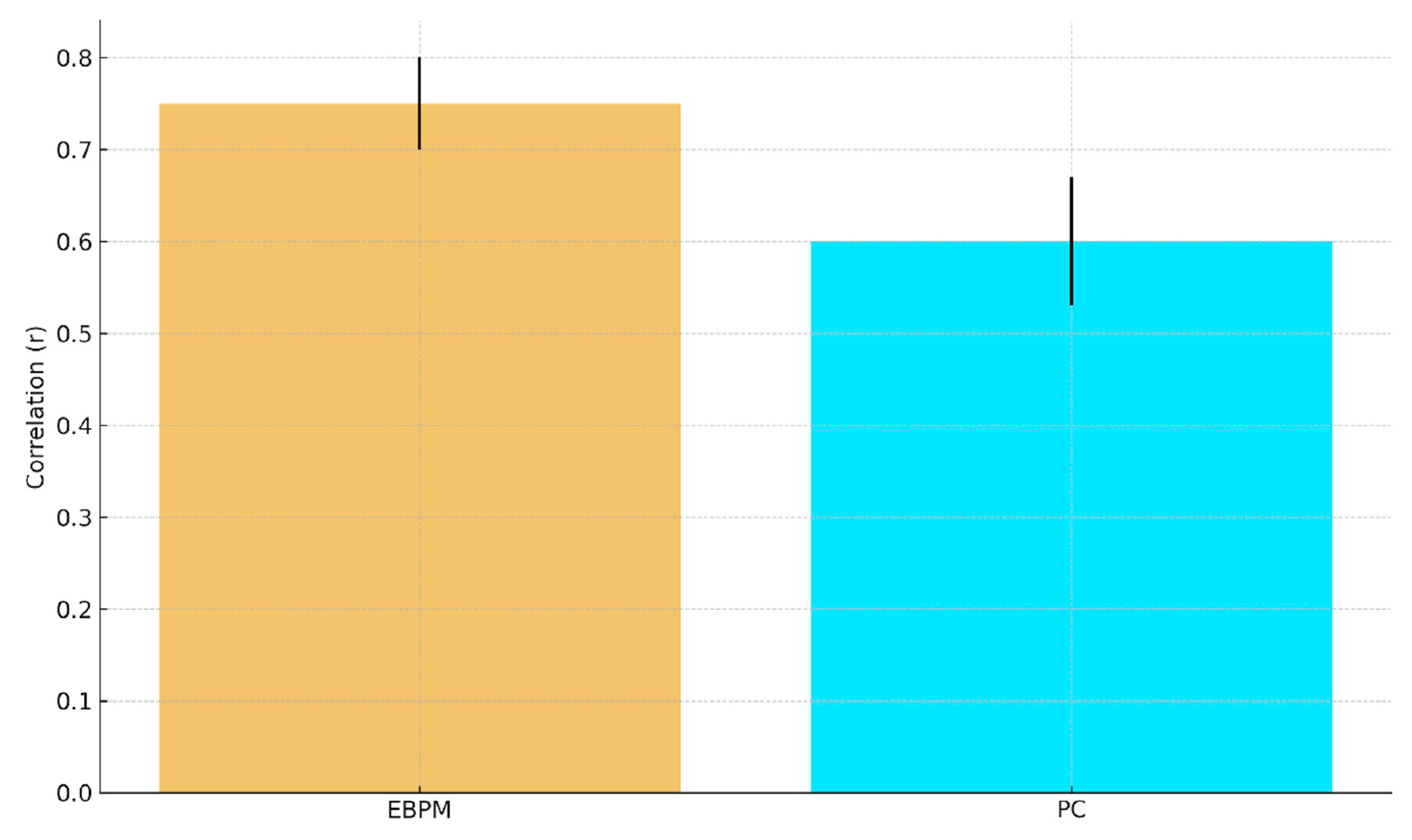
Figure E2.
a. Predicted ANN execution time (ms) with 95% CI: EBPM ≈ 80±10, PC ≈ 110±12.
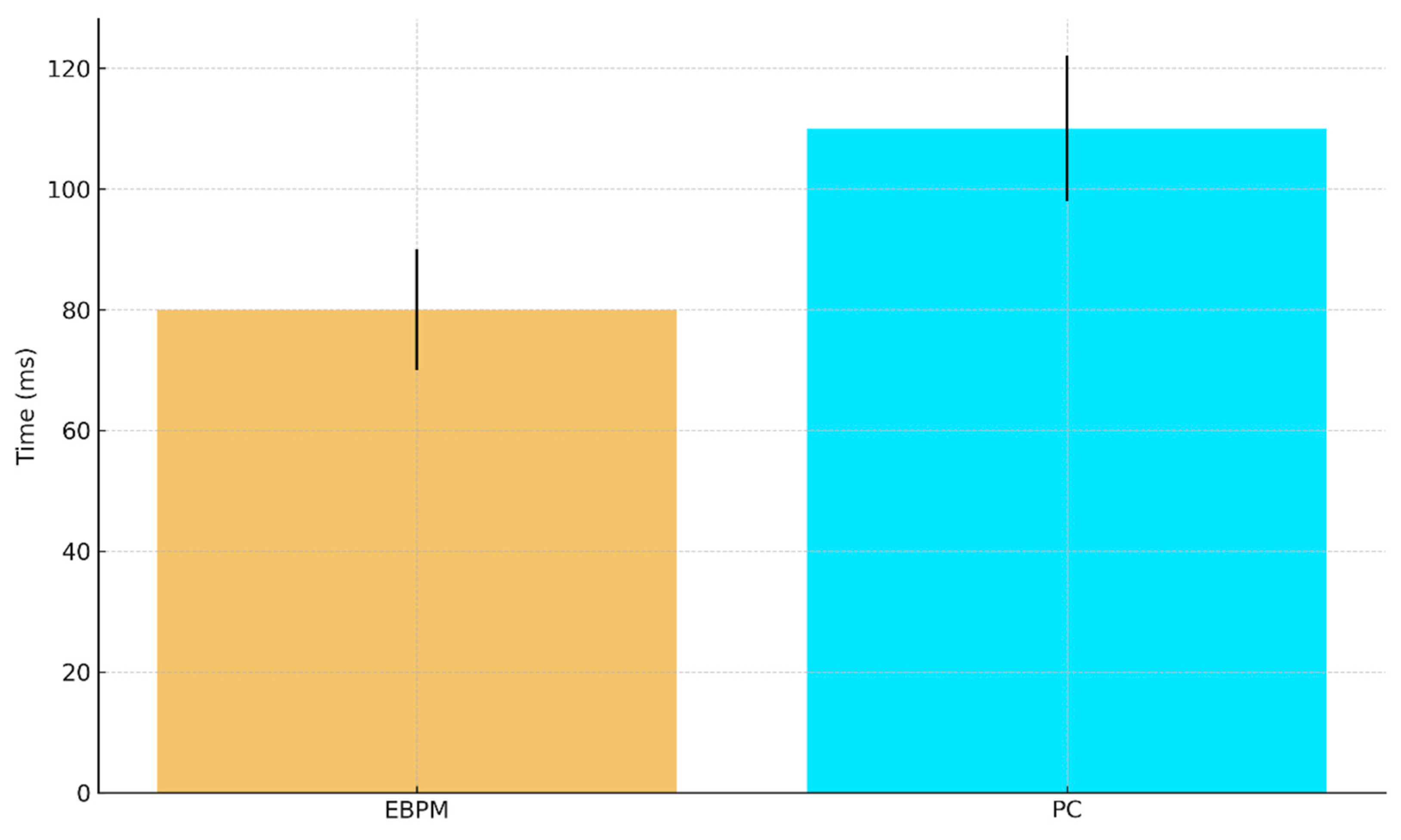
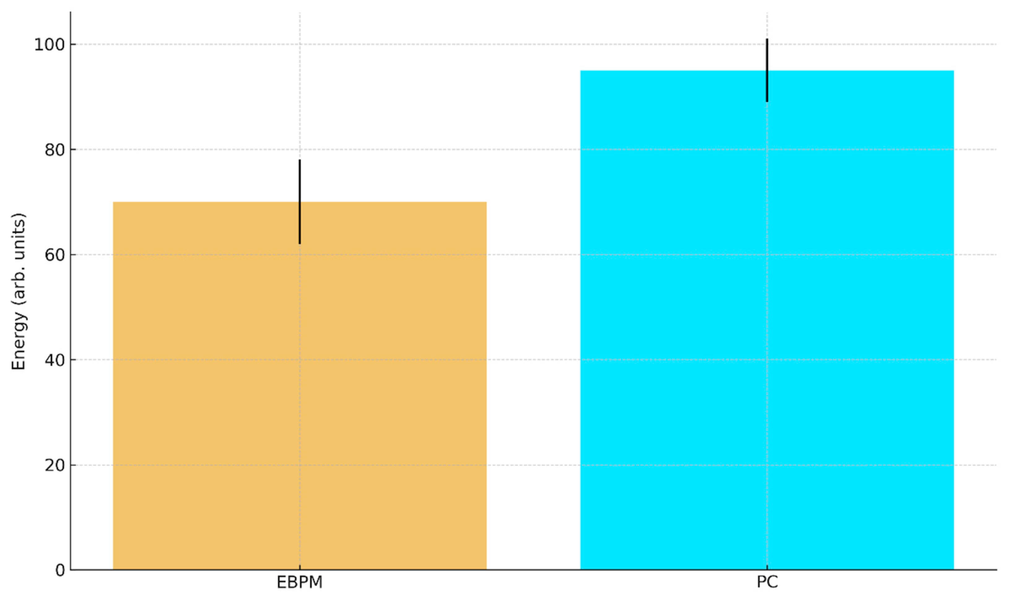
Figure E2.
b. Predicted robotic energy consumption (arb. units) with 95% CI: EBPM ≈ 70±8, PC ≈ 95±6.
Figure E2.
b. Predicted robotic energy consumption (arb. units) with 95% CI: EBPM ≈ 70±8, PC ≈ 95±6.
Appendix B
Table A1.
Rdata.
| File (relative path) | What it contains |
|---|---|
| results_csv/pybullet_obstacles_metrics_v3c_alpha.csv | v3c_alpha (α=0.65): ms/step mean, steps, success, collisions, avg PC calls per mode & noise |
| results_csv/pybullet_obstacles_metrics_v3c.csv | v3c (dyn gating, no fixed α): same fields |
| results_csv/pybullet_obstacles_metrics_v3b.csv | v3b: success & collisions breakdown |
| results_csv/pybullet_perception_metrics.csv | demo perception ms/step EBPM vs PC vs DIME |
References
- K. Friston. The free-energy principle: a unified brain theory? Nat. Rev. Neurosci. 2010, 11, 127–138. [Google Scholar] [CrossRef]
- R. P. N. Rao and D. H. Ballard. Predictive coding in the visual cortex: a functional interpretation of some extra-classical receptive-field effects. Nat. Neurosci. 1999, 2, 79–87. [Google Scholar] [CrossRef]
- R. Kanai, Y. Komura, S. Shipp, and K. Friston. Cerebral hierarchies: predictive processing, precision and the pulvinar. Philos. Trans. R. Soc. B Biol. Sci. 2015, 370, 20140169. [Google Scholar] [CrossRef]
- G. Buzsáki. Neural Syntax: Cell Assemblies, Synapsembles, and Readers. Neuron 2010, 68, 362–385. [Google Scholar] [CrossRef]
- J. Hawkins and S. Ahmad. Why Neurons Have Thousands of Synapses, a Theory of Sequence Memory in Neocortex. Front. Neural Circuits 2016, 10. [CrossRef]
- H. Markram, W. H. Markram, W. Gerstner, and P. J. Sjöström. Spike-Timing-Dependent Plasticity: A Comprehensive Overview. Front. Synaptic Neurosci. 2012, 4. [Google Scholar] [CrossRef]
- J. J. Hopfield. Neural networks and physical systems with emergent collective computational abilities. Proc. Natl. Acad. Sci. 1982, 79, 2554–2558. [Google Scholar] [CrossRef] [PubMed]
- J. L. McClelland, B. L. McNaughton, and R. C. O’Reilly. Why there are complementary learning systems in the hippocampus and neocortex: Insights from the successes and failures of connectionist models of learning and memory. Psychol. Rev. 1995, 102, 419–457. [Google Scholar] [CrossRef]
- T. J. Teyler and P. DiScenna. The hippocampal memory indexing theory. Behav. Neurosci. 1986, 100, 147–154. [Google Scholar] [CrossRef]
- E. T. Rolls. The mechanisms for pattern completion and pattern separation in the hippocampus. Front. Syst. Neurosci. 2013, 7. [Google Scholar] [CrossRef]
- R. M. Nosofsky. Attention, similarity, and the identification–categorization relationship. J. Exp. Psychol. Gen. 1986, 115, 39–57. [Google Scholar] [CrossRef]
- G. D. Logan. Toward an instance theory of automatization. Psychol. Rev. 1988, 95, 492–527. [Google Scholar] [CrossRef]
- A. Biederman. Recognition-by-components: A theory of human image understanding. Psychol. Rev. 1987, 94, 115–147. [Google Scholar] [CrossRef]
- P. Kanerva, Sparse distributed memory. Cambridge, Mass: MIT Press, 1988.
- I. Graves, G. Wayne, and I. Danihelka. Neural Turing Machines. 2014, arXiv. [CrossRef]
- A. Graves et al.. Hybrid computing using a neural network with dynamic external memory. Nature 2016, 538, 471–476. [Google Scholar] [CrossRef] [PubMed]
- A. Blundell et al.. Model-Free Episodic Control. 2016, arXiv. arXiv. [CrossRef]
- J. Snell, K. J. Snell, K. Swersky, and R. S. Zemel. Prototypical Networks for Few-shot Learning. 2017, arXiv. [CrossRef]
- I. Clark. Whatever next? Predictive brains, situated agents, and the future of cognitive science. Behav. Brain Sci. 2013, 36, 181–204. [Google Scholar] [CrossRef] [PubMed]
- A. M. Bastos, W. M. Usrey, R. A. Adams, G. R. Mangun, P. Fries, and K. J. Friston. Canonical Microcircuits for Predictive Coding. Neuron 2012, 76, 695–711. [Google Scholar] [CrossRef]
- A. A. Olshausen and D. J. Field. Emergence of simple-cell receptive field properties by learning a sparse code for natural images. Nature 1996, 381, 607–609. [Google Scholar] [CrossRef] [PubMed]
- Y. Bengio, A. Courville, and P. Vincent. Representation Learning: A Review and New Perspectives. IEEE Trans. Pattern Anal. Mach. Intell. 2013, 35, 1798–1828. [Google Scholar] [CrossRef]
- L. Itti and C. Koch. Computational modelling of visual attention. Nat. Rev. Neurosci. 2001, 2, 194–203. [Google Scholar] [CrossRef]
- G. Aston-Jones and J. D. Cohen. AN INTEGRATIVE THEORY OF LOCUS COERULEUS-NOREPINEPHRINE FUNCTION: Adaptive Gain and Optimal Performance. Annu. Rev. Neurosci. 2005, 28, 403–450. [Google Scholar] [CrossRef]
- S. Dehaene, F. Meyniel, C. Wacongne, L. Wang, and C. Pallier. The Neural Representation of Sequences: From Transition Probabilities to Algebraic Patterns and Linguistic Trees. Neuron 2015, 88, 2–19. [Google Scholar] [CrossRef] [PubMed]
- R. J. Douglas and K. A. C. Martin. Recurrent neuronal circuits in the neocortex. Curr. Biol. 2007, 17, R496–R500. [Google Scholar] [CrossRef] [PubMed]
- G. G. Ambrus. Shared neural codes of recognition memory. Sci. Rep. 2024, 14, 15846. [Google Scholar] [CrossRef]
- W. Gerstner, W. M. Kistler, R. Naud, and L. Paninski, Neuronal Dynamics: From Single Neurons to Networks and Models of Cognition, 1st ed. Cambridge University Press, 2014. [CrossRef]
- J. St. B. T. Evans and K. E. Stanovich. Dual-Process Theories of Higher Cognition: Advancing the Debate. Perspect. Psychol. Sci. 2013, 8, 223–241. [Google Scholar] [CrossRef]
- U. Hasson, J. Chen, and C. J. Honey. Hierarchical process memory: memory as an integral component of information processing. Trends Cogn. Sci. 2015, 19, 304–313, June. [Google Scholar] [CrossRef]
- A. Summerfield and F. P. De Lange. Expectation in perceptual decision making: neural and computational mechanisms. Nat. Rev. Neurosci. 2014, 15, 745–756. [Google Scholar] [CrossRef]
- P. Kok, J. F. M. Jehee, and F. P. de Lange. Less Is More: Expectation Sharpens Representations in the Primary Visual Cortex. Neuron 2012, 75, 265–270. [Google Scholar] [CrossRef]
- S. J. Kiebel, J. Daunizeau, and K. J. Friston. A Hierarchy of Time-Scales and the Brain. PLoS Comput. Biol. 2008, 4, e1000209. [Google Scholar] [CrossRef]
Figure 1.
Schematic representation of the EBPM framework.
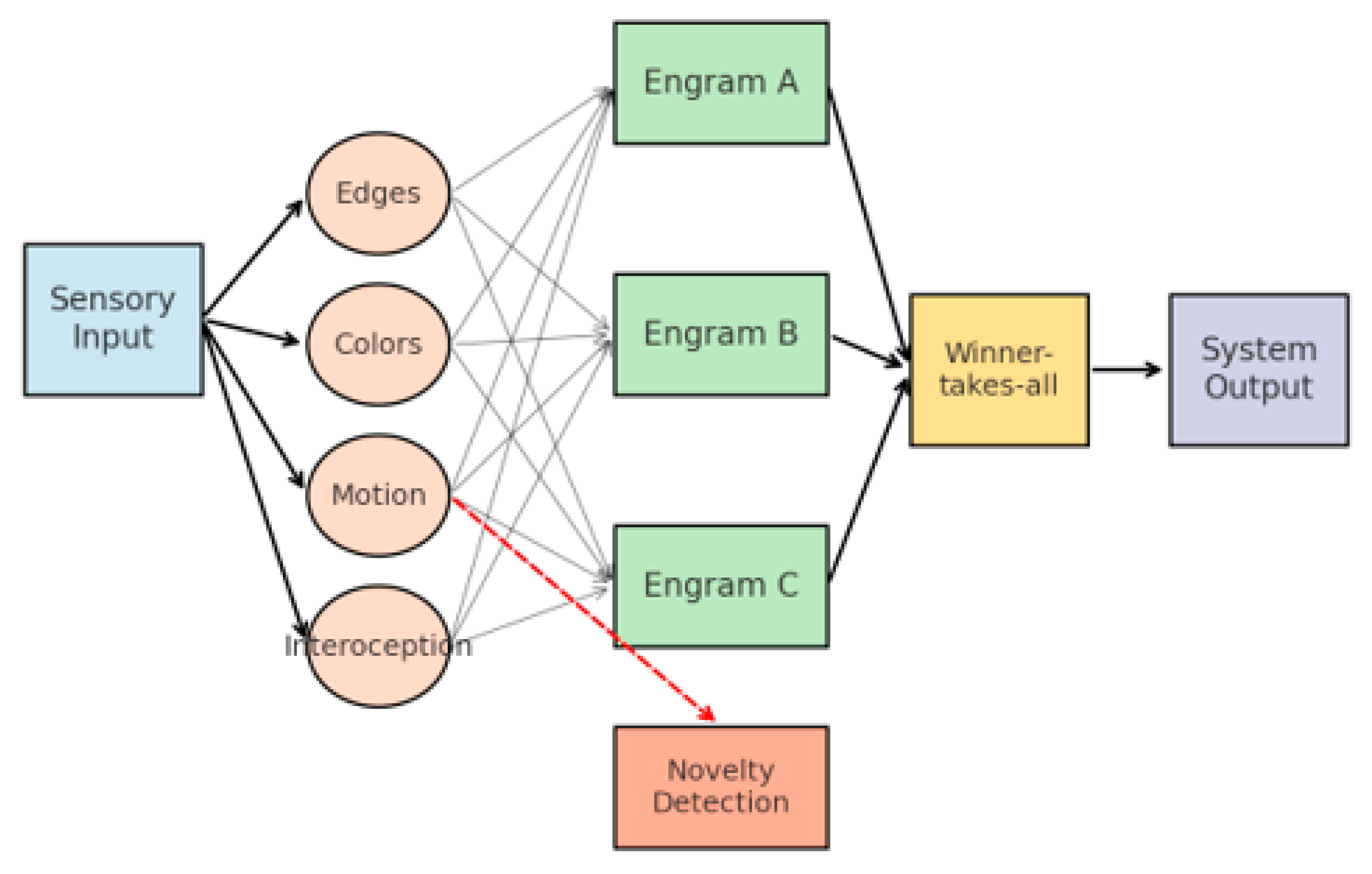
Figure 2.
Predictive Coding (PC) architecture.
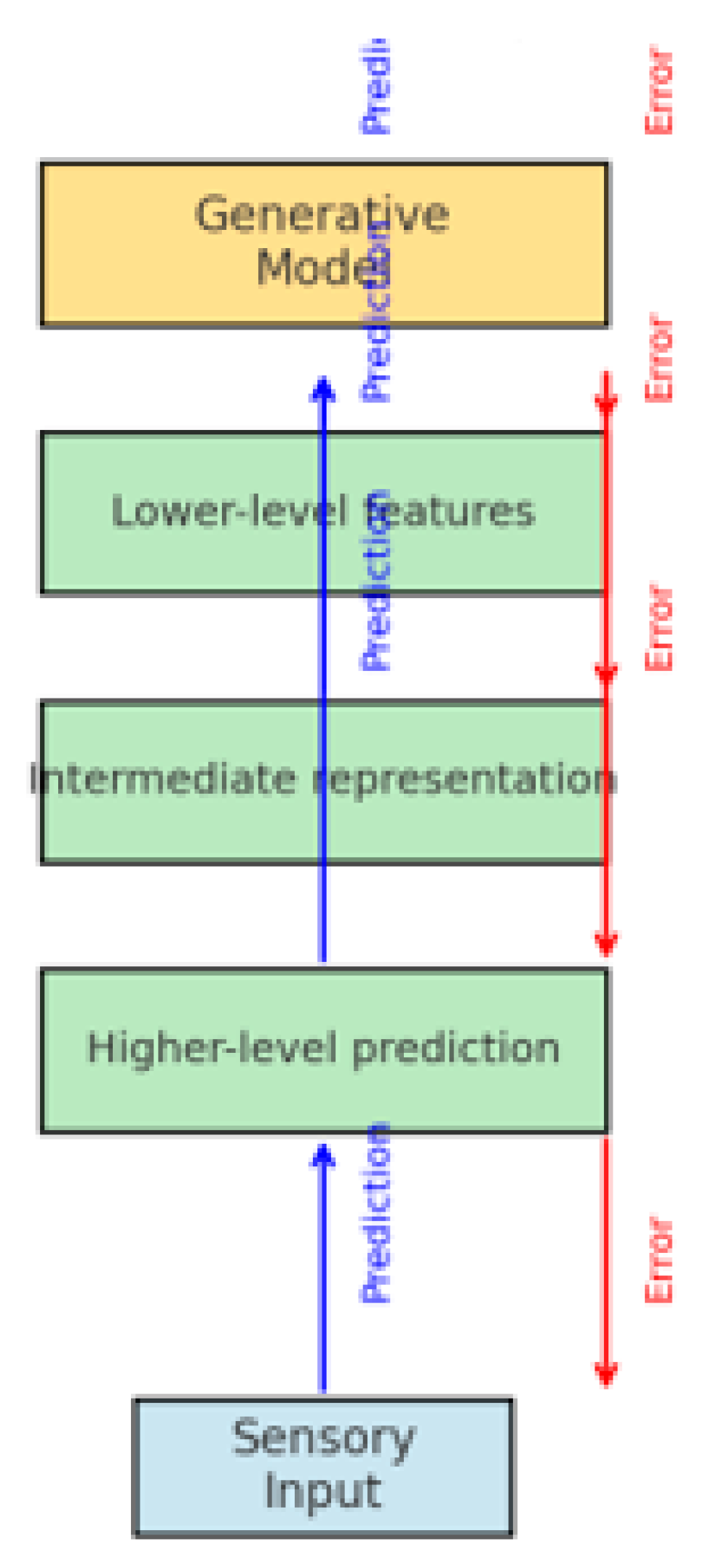
Figure 3.
DIME (Dynamic Integrative Matching and Encoding) model.
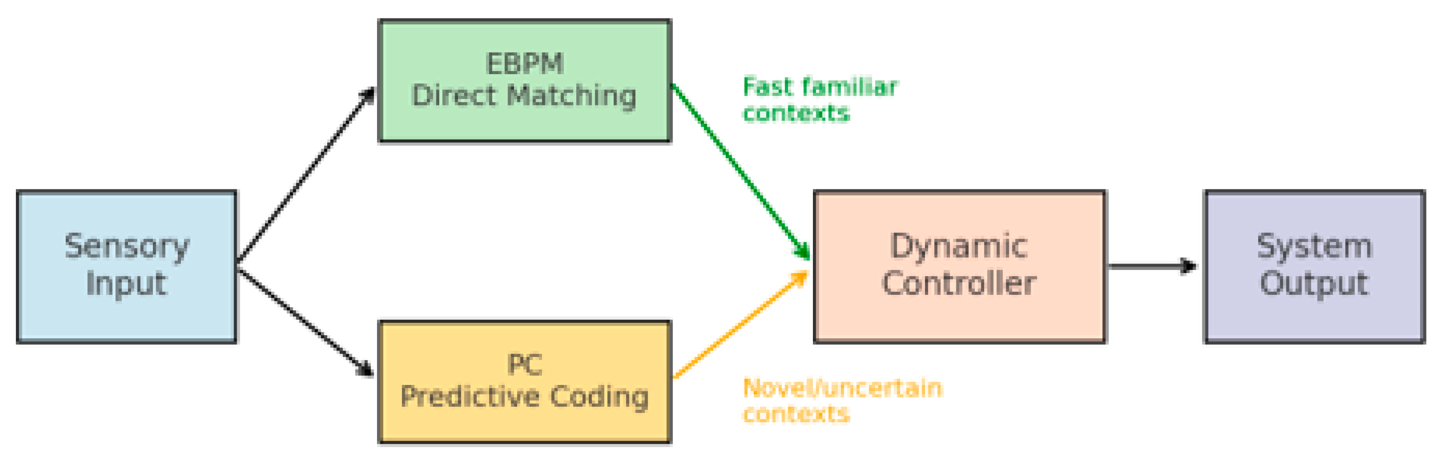
Figure 4.
Proposed experimental validation methodology.
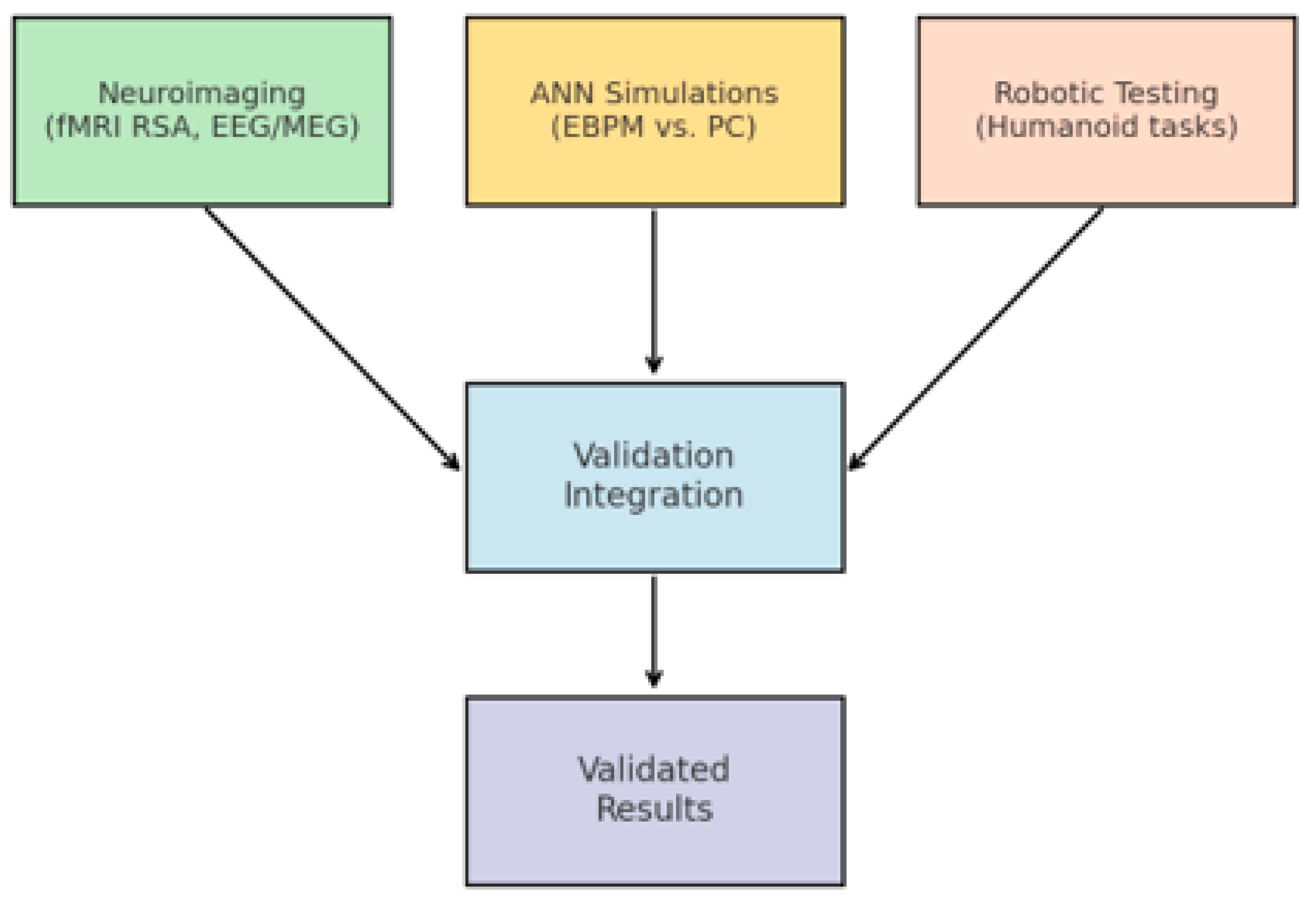
Figure 13.
General information flow in the DIME model.
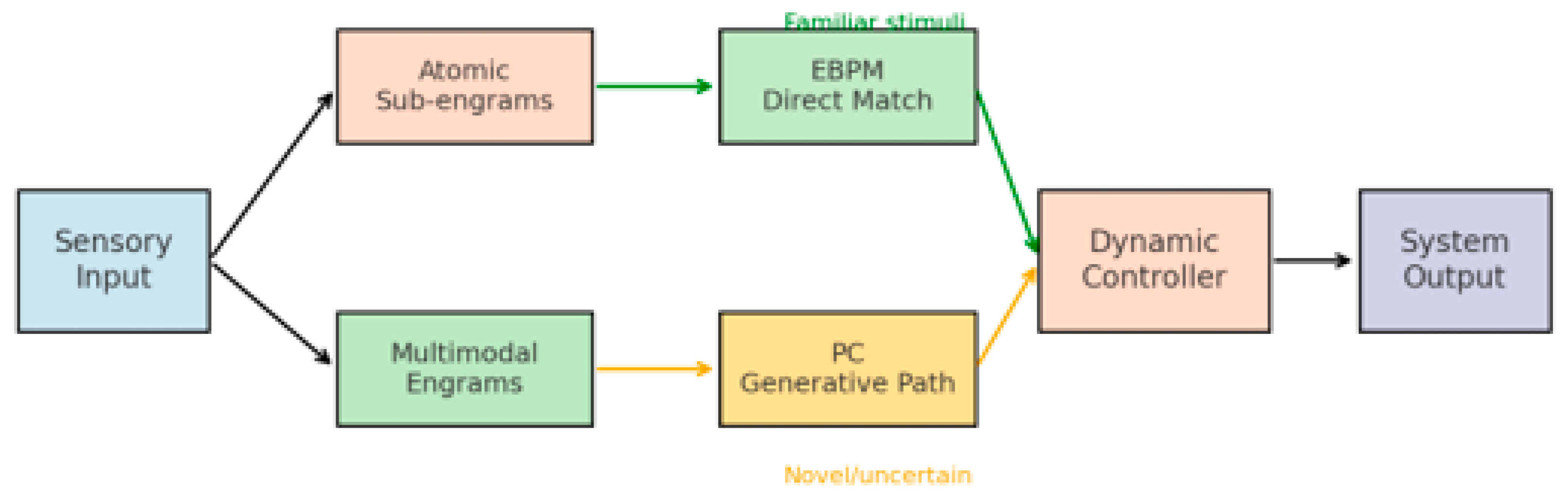
Figure 16.
Runtime cost vs. noise (v3c_alpha, α=0.65). Mean perception time per step (3 episodes) for EBPM, PC, DIME, and DIME-Lazy, under noise ∈ {0.0, 0.15}. DIME-Lazy equals EBPM on stable frames and escalates to PC under higher dynamics, preserving 100% success.
Figure 16.
Runtime cost vs. noise (v3c_alpha, α=0.65). Mean perception time per step (3 episodes) for EBPM, PC, DIME, and DIME-Lazy, under noise ∈ {0.0, 0.15}. DIME-Lazy equals EBPM on stable frames and escalates to PC under higher dynamics, preserving 100% success.
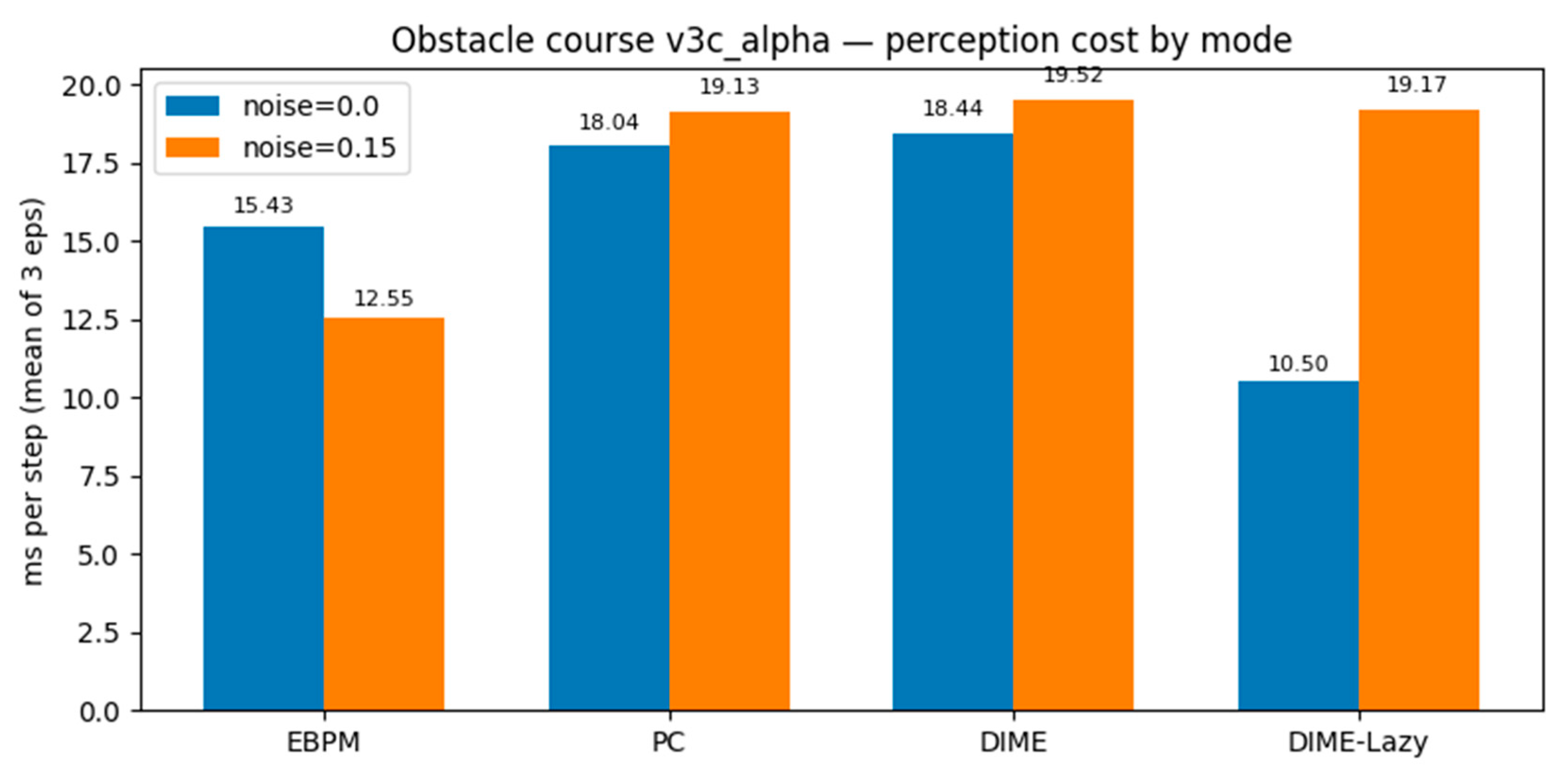
Figure 17.
Runtime cost & PC calls (two-panel summary). Left: ms/step (mean of 3 episodes). Right: average #PC calls. Runtime-aware gating reduces cost on stable scenes and increases it when dynamics/noise rise, with unchanged task success.
Figure 17.
Runtime cost & PC calls (two-panel summary). Left: ms/step (mean of 3 episodes). Right: average #PC calls. Runtime-aware gating reduces cost on stable scenes and increases it when dynamics/noise rise, with unchanged task success.
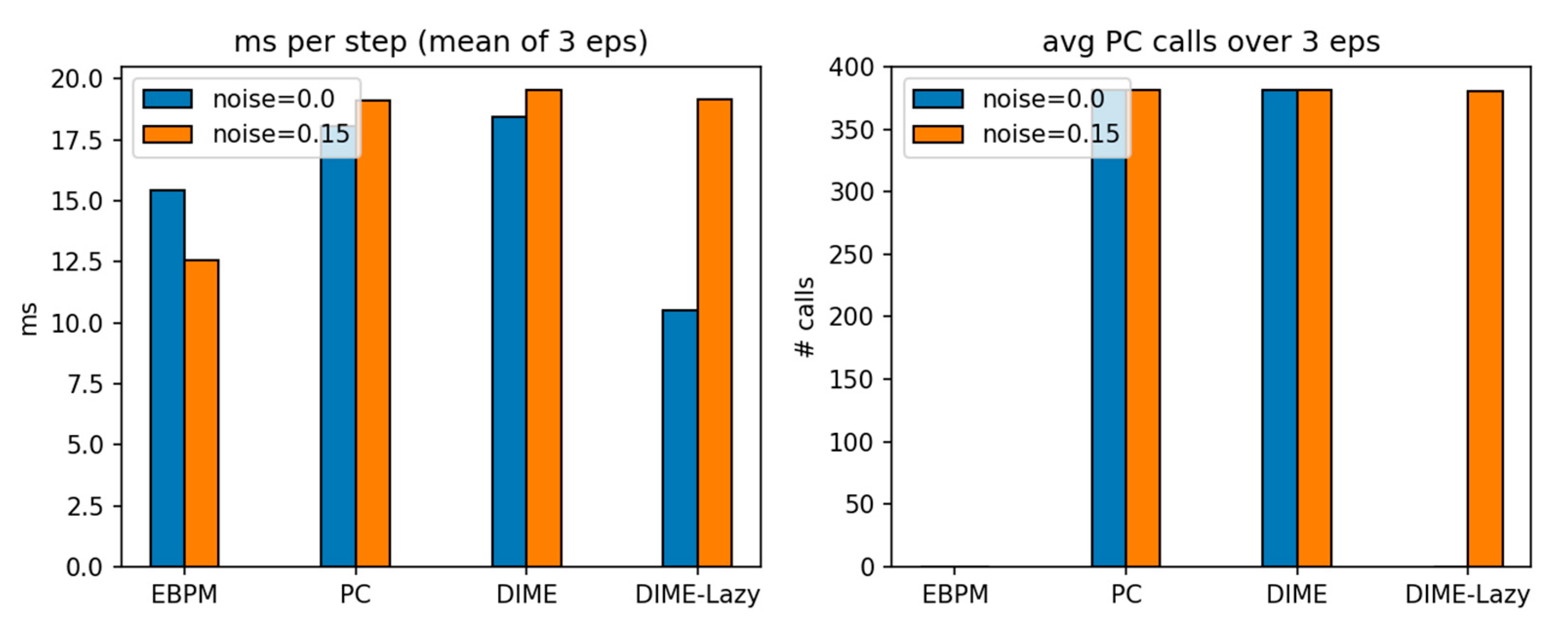
Table 7.
Strengths and limitations of EBPM, PC, DIME.
| Aspect | EBPM | PC | DIME |
|---|---|---|---|
| Speed | High | Medium | High |
| Energy Efficiency | High | Low | Medium–High |
| Noise Robustness | Medium-Low | High | High |
| Flexibility | Low | High | High |
| Biological Plausibility | High | Medium | High |
Disclaimer/Publisher’s Note: The statements, opinions and data contained in all publications are solely those of the individual author(s) and contributor(s) and not of MDPI and/or the editor(s). MDPI and/or the editor(s) disclaim responsibility for any injury to people or property resulting from any ideas, methods, instructions or products referred to in the content. |
© 2025 by the authors. Licensee MDPI, Basel, Switzerland. This article is an open access article distributed under the terms and conditions of the Creative Commons Attribution (CC BY) license (http://creativecommons.org/licenses/by/4.0/).
Copyright: This open access article is published under a Creative Commons CC BY 4.0 license, which permit the free download, distribution, and reuse, provided that the author and preprint are cited in any reuse.


