
Submitted:
10 September 2025
Posted:
12 September 2025
You are already at the latest version
Abstract
In recent years, Positive Energy Districts (PEDs) have been interpreted in many—and often conflicting—ways. This breadth has limited traction: projects defined disparate “energy-positive” metrics that were not directly tied to Paris-aligned climate neutrality. We recast PEDs as a vehicle for verifiable climate neutrality and present a declaration-ready assessment that integrates (i) a cumulative, science-based GHG budget per m² gross floor area (GFA), (ii) full life-cycle accounting, and (iii) time-resolved operational factors that include everyday motorized individual mobility (EMIM) and quantify flexibility. Two KPIs anchor the framework: the cumulative GHG LCA balance (2025–2075) against a maximum compliant budget of 320 kgCO₂e·m⁻²GFA and the annual primary-energy (PE) balance used to declare PED status with or without mobility. We follow EN 15978 system logic with PED-oriented refinements—certain biogenic storage, PV→grid substitution crediting, and omission of project-level PV embodied impacts—and apply time-resolved emission factors that decline to zero by 2050. Under this assumption, most GHG accounting past 2050 ceases to be decision-relevant; the framework’s obligation is to stay within the 2025–2050 budget. Its applicability is demonstrated on six Austrian districts spanning new build and renovation, diverse energy systems, densities, and mobility contexts. Baseline scenarios show heterogeneous outcomes—only some meet both the cumulative GHG budget and the positive primary-energy balance—but design iterations indicate that all six districts can reach the targets with realistic, ambitious packages (e.g., ecological material substitutions, PV oversizing with flexibility, GSHP/TABS, BESS/V2B, and mobility electrification/demand reduction). Hourly emission factors with rolling-average flexibility signals can materially lower import-weighted emission intensity versus monthly or annual factors and reveal seasonal import–export asymmetries that annual bookkeeping masks. Built on transparent, auditable rules and open tooling, this framework both diagnoses performance gaps and maps credible pathways to compliance—steering PED design away from project-specific targets toward verifiable climate neutrality. It now serves as the basis for a national labeling/declaration scheme, enabling broad, consistent adoption across projects.
Keywords:
Positive Energy Districts (PEDs)
; Climate neutrality assessment
; Greenhouse gas (GHG) emissions
; Life-cycle assessment (LCA)
; Embodied and operational emissions
; Building energy systems
; Mobility emissions
1. Introduction
Achieving climate neutrality by mid-century, as stipulated under the Paris Agreement [1], requires rapid and deep decarbonization across all sectors. The IPCC Sixth Assessment Report confirms that limiting warming to 1.5 °C necessitates stringent carbon budgets, with global net-zero CO₂ emissions reached around [2,3,4,5]. The building sector is pivotal in this transition, contributing significantly to both operational greenhouse gas (GHG) emissions and embodied emissions from construction and refurbishment [6,7].
Positive Energy Districts (PEDs) are increasingly promoted as a transformative model to support this transition, integrating high energy efficiency, local renewable generation, and energy flexibility to achieve an annual net-positive energy balance [8,9,10,11]. However, an energy surplus alone does not automatically ensure alignment with national or global climate targets, particularly those consistent with the Paris Agreement [3]. Climate neutrality requires aligning emissions with a finite, science-based GHG budget that limits global warming to 1.5 °C (or well below 2 °C), necessitating a lifecycle-based approach that captures embodied emissions, biogenic carbon flows, and time-resolved operational emissions [7]. Existing net-zero building and zero-emission neighborhood frameworks rarely translate cumulative, sector-specific CO₂ budgets into explicit floor-area-specific targets [12]. At the PED scale, three main challenges emerge:
Life cycle assessment (LCA) standards, particularly EN 15978:2024 [19], provide a robust structure for defining system boundaries and modules for embodied and operational emissions in buildings and districts. Previous work [16,18,20,21,22] highlights the need to adapt these methods to the district scale while ensuring compatibility with sectoral carbon budgets. Dynamic emission factors—which reflect the projected decline in grid and district heating carbon intensities—are essential for accurately representing operational impacts over time [23]. International studies [24,25] demonstrate the influence of such temporal factors on lifecycle results, and highlight differences in the treatment of embodied emissions of energy infrastructure.
Against this background, this proposed climate neutrality assessment framework for PEDs builds on the established Positive Energy District assessment framework described in [14] and further developed in the simulation and evaluation methodology of [26]. Building on EN 15978 system boundaries, it integrates dynamic, energy-carrier-specific emission factors and operationally includes everyday motorized individual mobility (EMIM) and embodied emissions from construction and maintenance from now until 2050. Within the broader assessment framework, this paper addresses the climate neutrality and life-cycle carbon accounting dimension, complementing the framework’s energy system modelling and flexibility evaluation capabilities presented in earlier work [14,26]. The shared objective is to provide a methodologically rigorous yet practice-ready approach that captures both (i) the operational responsiveness of PEDs to system needs and (ii) their compliance with carbon budgets consistent with Austria’s 2040 climate neutrality target.
The framework presented here is designed to be robust for research purposes—allowing sensitivity analyses with hourly emission factors—while remaining compatible with the monthly conversion factors of the Austrian building code for practical declarations of climate-neutral PEDs as part of the Austrian sustainability label family klimaaktiv [27]. Its core contribution is the derivation of a quantifiable carbon budget per square meter of gross floor area (GFA), integrating both operational and embodied emissions in a manner that is directly linkable to the performance outcomes of the broader PED assessment framework.
Study Contribution
This study extends the established Positive Energy District (PED) assessment framework [14,26] by operationalizing climate neutrality through life-cycle carbon accounting and science-based carbon budgets. It (i) applies a life cycle GHG accounting method consistent with national decarbonization pathways, (ii) incorporates time-differentiated operational emission factors for multiple energy carriers, and (iii) integrates everyday motorized individual mobility as part of project-level design. Anchoring the method in a tested PED framework ensures alignment with established definitions and simulation methodologies, while enabling integrated evaluations in which life-cycle carbon compliance can be assessed alongside energy performance and flexibility metrics.
2. Materials and Methods
2.1. Methodological Principles
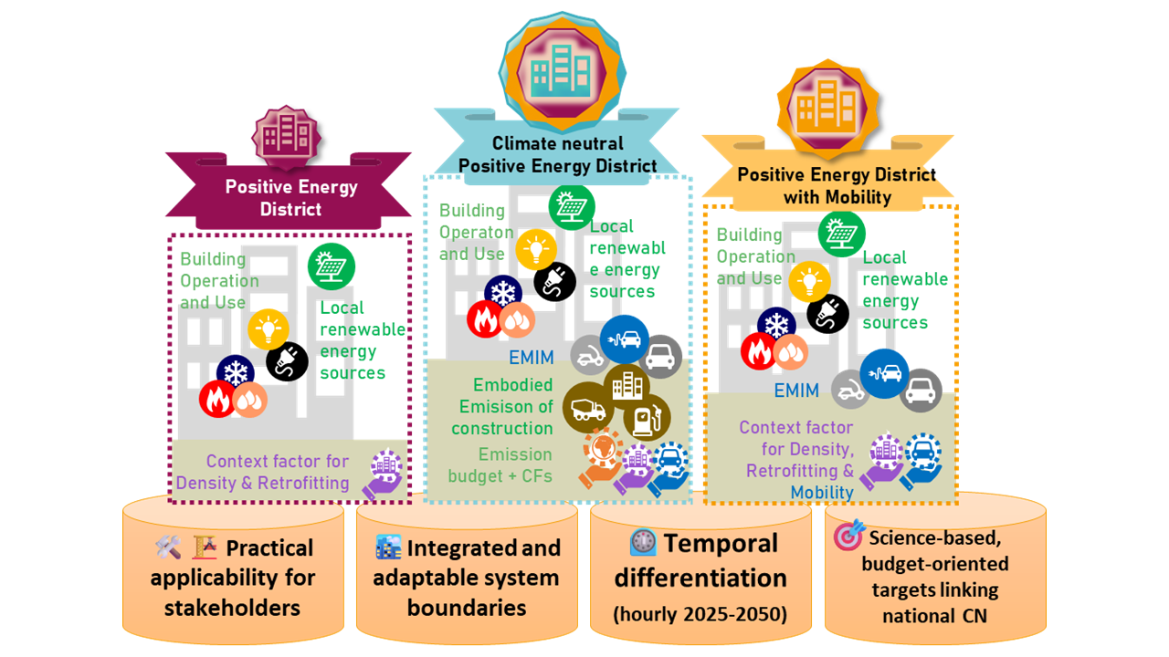
The proposed climate neutrality assessment framework is grounded in a set of guiding principles that combine practical applicability with scientific rigor, ensuring relevance for both practitioners and researchers.
- Practical applicability and stakeholder relevance – The method is designed to be appliable for real estate developers, municipalities, and planning professionals, enabling its integration into certification schemes and project assessments [28,29,30,31]. Its scope is limited to emissions that can be directly influenced through planning and construction decisions—namely, operational energy use, EMIM, and embodied emissions—ensuring decision-making relevance.
- Integrated and adaptable system boundaries – Assessment boundaries extend beyond individual buildings to the full Positive Energy District (PED) system, covering on-site generation, storage, flexibility, and interconnections with surrounding grids. The framework retains adaptability in data sources, emission factors, and system configurations, allowing regional customization while ensuring methodological comparability.
- Temporal differentiation – Emissions are assessed over a 50-year timeframe (2025–2075), with the assumption that climate neutrality is achieved for all services by 2050. As a result, all conversion factors for both operational and embodied energy are assumed to be zero by 2050, reflecting the expected decarbonization of energy carriers and building systems. This approach ensures alignment with long-term climate goals while considering the gradual reduction of emissions over the assessment period.
- Science-based, budget-oriented compliance thresholds – The method is anchored in downscaled CO₂ budgets consistent with Austria’s 2040 climate neutrality target and the 1.5 °C global carbon budget [1]. It establishes a hierarchy of compliance thresholds: an ambitious target value representing a precautionary level for high-confidence Paris alignment, and a maximum compliance limit that must not be exceeded for a project to qualify as “climate-neutral PED.”
These principles acknowledge that PED definitions inherently allow for multiple interpretations, particularly regarding system boundaries, included emission sources, and treatment of temporal dynamics. As noted in prior work [14,32], these degrees of freedom can lead to inconsistent assessments if not addressed explicitly. The framework therefore applies a design thinking approach to close such gaps: key methodological choices—such as which life cycle stages to include, how to allocate renewable generation, and how to integrate mobility—are made transparent, justified against policy and scientific references, and consistently applied.
Figure 1.
Methodological Approach to design of climate neutrality definition for PEDs is based on four pillars, on which three practical PED definitions are based (boxes show conceptualized functional system boundaries).
Figure 1.
Methodological Approach to design of climate neutrality definition for PEDs is based on four pillars, on which three practical PED definitions are based (boxes show conceptualized functional system boundaries).
The following section details how these methodological principles are operationalized within the proposed framework, from KPI definition and the derivation of target carbon budgets to the application of dynamic emission factors and the inclusion of mobility and embodied emissions.
2.2. Key Performance Indicators (KPIs) and PED Levels
We base our assessment framework on two main indicators as defined in [14]:
- Cumulative GHG balance (2025–2075, kgCO₂e·m⁻²GFA) — as defined in the framework above: cradle-to-grave embodied emissions (A1–A3; buildings, TES, PV, batteries, vehicles, C1-C4 before 2050), time-resolved operational emissions (B6; grid electricity and thermal carriers), operational mobility (B8 EMIM; ICE/EV), and avoided grid emissions (D2; PV exports and EMIM substitution). Negative components reduce the balance. Compliance bands are L3 = 320, L2 = 196, L1 = 72 kgCO₂e·m⁻²GFA.
- Primary-energy (PE) balance (kWhₚₑ·m⁻² NFA·a-1) — computed per [14,26] as the difference between annual primary-energy grid equivalence from local renewable supply and flexible grid use (PV self-use and feed-in, flexible TES and EMIM operation) and the district’s primary-energy demand (grid equivalence, HVAC and electricity; EMIM included or excluded depending on the level). A positive value denotes a “positive balance”. Context factors for density, mobility and renovation may apply as virtual demands or supplies.
These two KPIs are reported consistently across case studies; figures annotate overshoot/undershoot against L-levels, and tables list the corresponding PE balances. Operational energy KPIs are expressed per conditioned Net Floor Area (NFA) because heating, cooling, and end-use electricity demands are specified for conditioned area in design practice and codes, so NFA best matches how these targets are set and tracked. Lifecycle GHG indicators are expressed per Gross Floor Area (GFA) to maintain comparability across typologies and density/fit-out choices; NFA↔GFA conversions are straightforward via use-type factors that are routinely applied (and refined from early planning estimates). Based on these indicators, we distinguish three PED levels as shown in Table 1:
Results are compiled with the scenario analysis tools provided by the framework (publicly available here [33]).
2.3. Carbon Budget for Climate-Neutral Districts
We derive project-level carbon budgets by downscaling a finite, Paris-compatible global CO₂ budget to Austria (national), then allocating a sectoral share to buildings (construction, operation, everyday motorized mobility), translating per-capita values to floor-area–specific targets using national floor space statistics. We adopt the +1.5 °C, 66% probability case and add natural sink assumptions of 0.5 and 1.0 t CO₂ cap⁻¹ a⁻¹. The resulting floor-area budgets define three compliance levels:
- Target value (L1) — conservative Paris-compatible target (strict),
- Precautionary limit (L2) — with 0.5 t CO₂ cap⁻¹ a⁻¹ sinks,
- Compliance limit (L3) — with 1.0 t CO₂ cap⁻¹ a⁻¹ sinks.
Derivation. We compute floor-area–specific cumulative budgets for 2025–2075 as follows:
- Global → national budget (2025–2075). Starting from the remaining global/national CO₂ budgets in 2022 [17], we subtract realized emissions in 2022–2024 to obtain the remaining 2025–2075 budget under two variants: (i) +5 °C without overshoot (50% and 66% probability) and (ii) +5 °C with temporarily higher temperatures (50% and 66%).
- National → sectoral, per capita (net). The national budget is allocated to the buildings/EMIM sector according to [16] and expressed per capita, yielding a net emission budget (i.e., excluding natural sinks).
- Add natural carbon sinks (gross). We then add natural carbon sinks of 1.0 t CO₂ cap⁻¹ a⁻¹ (based on [34] and, for sensitivity, 0.5 t) to obtain the gross per-capita budgets over 2025–2075.
- Per-m² metric. The per-capita gross budget is converted to a floor-area–specific limit using national GFA statistics (all uses). This yields the compliance limit L3 ≈ 320 kg CO₂e m⁻²GFA (2025–2075); L2 and L1 follow from the same chain under the stricter sink/overshoot assumptions (see Table 1).
Resulting budgets are expressed as cumulative lifecycle greenhouse gas (GHG) emissions from 2025 to 2050, integrating both operational and embodied sources. (see Table 3). These limits distinguish between an ambitious Paris-compatible target and two compliance thresholds based on sequestration assumptions (0.5 and 1.0 t CO₂/year/person). The framework requires that projects remain below at least the absolute compliance limit to qualify as climate neutral, with the precautionary limit recommended as a more robust operational benchmark.

Table 2.
Carbon budget inputs and derived per-capita/per-area values (2025–2075).
| Variable | Unit | Timeframe | 50% | 66% | Source |
| Paris-compatible CO₂ budget (+1.5 °C, no overshoot) | Mt CO₂ | 2022–2075 | 510 | 280 | [17] |
| Paris-compatible CO₂ budget (+1.5 °C, with overshoot) | Mt CO₂ | 2022–2075 | 610 | 340 | [17] |
| Remaining budget after 2024 (no overshoot) | Mt CO₂ | 2025–2075 | 360 | 130 | calc. from [17] |
| Remaining budget after 2024 (with overshoot) | Mt CO₂ | 2025–2075 | 460 | 190 | calc. from [17] |
| Population (Austria) | million cap | 2025 | 9.0 | 9.0 | [27] |
| Per-capita net budget (no overshoot) | t CO₂ cap⁻¹ | 2025–2075 | 40.0 | 14.5 | calc. from [37] |
| Per-capita net budget (with overshoot) | t CO₂ cap⁻¹ | 2025–2075 | 51.1 | 21.1 | calc. from [37] |
| Natural carbon sinks (NCS) | t CO₂ cap⁻¹ a⁻¹ | — | 1.0 | 1.0 | [6] |
| Cumulative NCS added (50 years) | t CO₂ cap⁻¹ | 2025–2075 | 50.0 | 50.0 | — |
| Per-capita gross budget (no overshoot + NCS) | t CO₂ cap⁻¹ | 2025–2075 | 90.0 | 64.5 | — |
| Per-capita gross budget (with overshoot + NCS) | t CO₂ cap⁻¹ | 2025–2075 | 101.1 | 71.1 | — |
| Buildings + EMIM sector share of per-Capita budget (A1–A3, B1–B6 + EMIM, C1-C4) | % | — | 50 | 50 | [38] |
| Estimated national GFA (all uses) | million m² GFA | 2040 | 906.7 | 906.7 | [39] |
| Specific GFA per capita (all uses) | m² GFA cap⁻¹ | — | 101 | 101 | calc from [39] |
Table 3.
Target and compliance budget limits for climate-neutral Positive Energy Districts (PEDs) in Austria, expressed per gross floor area (GFA). Values are derived from Austria’s 2040 climate neutrality target, building stock data [39], and global carbon budget assumptions (+1.5 °C scenario, 66% probability; [17]).
| Limit | Value | Unit | Description & compliance note | ||
|
Paris-compatible target limit (GHG L1) |
72 | kgCO₂e·m-²GFA | Stringent, science-based carbon budget based on [2,17] ensuring a safe pathway to 1.5 °C. Assumes no contribution from biogenic carbon sequestration. Achieving this limit provides the highest certainty of Paris alignment but is challenging in practice. | ||
|
Precautionary compliance limit (GHG L2) |
196 | kgCO₂e·m-²GFA | Upper bound for climate-neutral declaration, assuming 0.5 tCO₂e·a-1·cap-1 sequestration. Offers flexibility while retaining a safety buffer; exceeding this value increases risk of overshooting Paris-compatible budgets. | ||
|
Absolute compliance limit (GHG L3) |
320 | kgCO₂e·m-²GFA | Maximum permissible budget, assuming 1 tCO₂e·a-1·cap-1 global sequestration. Exceeding this value disqualifies a PED from climate-neutral status under this framework. | ||
2.4. LCA System Boundary and Scope of District
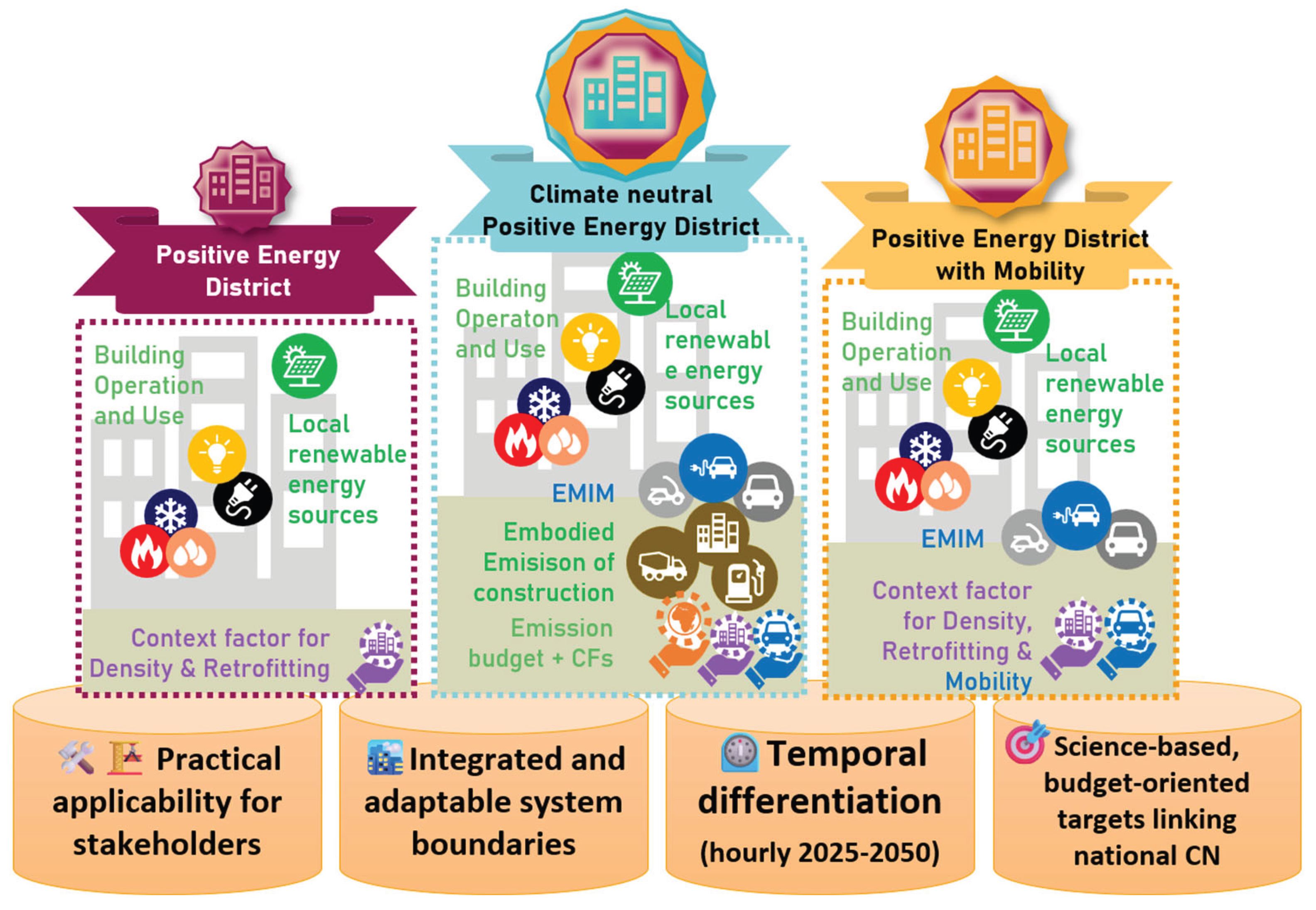
This section defines the temporal and functional boundaries for life-cycle assessment (LCA) within this proposed climate-neutrality assessment framework for PEDs. Unless stated otherwise, the assessment horizon is 2025–2075. All operational conversion factors decline to zero by 2050 for carriers on a national decarbonization pathway (e.g., electricity, district heating,); end-of-life and post-2050 processes are assumed carbon-neutral.
Figure 2.
System boundaries and scope of the life-cycle assessment (LCA), covering 2025–2075 and including both operational and construction emissions. Operational emissions comprise grid electricity use and substitution as well as other carriers (natural gas, biomass, fossil, district heating and cooling), with annual decarbonization of conversion factors to zero by 2050 where applicable. Construction emissions (A1–A3, B2–B5) account for certain biogenic carbon storage in bio-based material.
The assessment adapts life-cycle boundaries based on EN 15978 [19], with notable alterations: Unlike EN 15978, which references the EN 15804 [40] product standard that books stored biogenic CO₂ as an emission, this framework employs a time-dynamic LCA method for detailed declarations (Section 2.5.1). For practicability, a second, simplified method (section 2.5.2) can also be used, which credits biogenic carbon in building materials in part as carbon storage (negative emissions, 55%-100% depending on its origin and turnover period) over the horizon.
For mobility emissions, the framework includes parts of B8 that correspond to EMIM travels to the district and embodied emissions for vehicle construction (section 2.4.2).
Table 2 gives an overview of the concrete system boundary inclusions and exclusions:
Table 4.
System boundaries of Life Cycle Stage Inclusion in the assessment framework.
| Life Cycle Stage | Sub-stage | Module | Considered | Notes/Comments |
| A – Pre-construction | Pre-construction | A0 | No | Outside EN 15978 scope here |
| A – Product stage | Product stage | A1 | Yes | Raw material supply (embodied) |
| A2 | Yes | Transport to manufacturing | ||
| A3 | Yes* | Manufacturing emissions | ||
| A – Construction process stage | Construction | A4 | Yes* | Not assessed (practicability/data) |
| A5 | Yes | Not assessed (site installation) | ||
| B – Use stage | Use (non-energy) | B1 | No | Not considered |
| Maintenance | B2 | Yes* | Included; post-2050 assumed carbon-neutral | |
| Repair | B3 | Yes* | Same as B2 | |
| Replacement | B4 | Yes* | Same as B2 | |
| Refurbishment | B5 | Yes* | Same as B2 | |
| Operational energy use | B6 | Yes | Dynamic/Monthly factors (to 0 by 2050) | |
| Operational water use | B7 | No | Water-related GHG excluded | |
| Other building-related activities | B8 | Partly | EMIM B8.1 and B8.2 included (Section 2.4.2) Operational mileage + one-time vehicle embodied (≤2050) | |
| C – End-of-life stage | End-of-life | C1 | Yes | Included; post-2050 carbon-neutral |
| C2 | Yes | Same as C1 | ||
| C3 | Yes | Same as C1 | ||
| C4 | Yes | Same as C1 | ||
| D – Beyond system boundary | Reuse/recycling recovery | D1 | Yes | |
| Exported utilities | D2 | Yes | PV grid feed in credited as substitution with negative hourly/monthly factors | |
| Contextual | Off-plot public infrastructure | — | No | Optional reporting only (not for compliance) |
To ensure consistent coverage of embodied and operational impacts, the framework uses building balance boundary BB6 ([41], Table 3) for A1–A3 (product stage), B2–B5 (use stage) and End-of-life prior to 2050 (C1-C4). BB6 covers the complete building: thermal envelope, interior partitions, basement structures, unheated buffer zones, technical systems, and exterior facilities (carports, bicycle shelters, auxiliary buildings).
Table 5.
Building LCA balancing boundaries [41].
Table 5.
Building LCA balancing boundaries [41].
| Boundary | Scope description |
| BB1 | Complete thermal envelope, including internal floor ceilings |
| BB3 | BB1 plus all interior walls, basement structures, unheated buffer zones; excluding open circulation spaces (stairs, balconies, loggias, galleries) |
| BB5 | BB3 plus shared circulation areas and building services |
|
BB6 (used here) |
BB5 plus exterior facilities (carports, bicycle shelters, etc.) and auxiliary buildings |
2.4.1. Local PV and Exported Electricity (Module B6 / D2)
Local PV is handled operationally only: on-site generation replaces grid electricity using the framework’s conversion factors (hourly for analysis and optimization; monthly building-code factors for declarations). Surplus feed-in is credited as grid substitution potential (Module D2) using the same operational factors. This means that for declaration GHG and PE accounting purposes, feed in and self-consumption are equivalent. For research and future iterations of declarations, this can be detailed by setting the feed-in grid substitution factor to an appropriate / time-dependent fraction of the grid import factor.
Embodied impacts of PV systems are not counted at project level, as they are allocated to the national energy sector that underlies both the budget derivation and the operational factors used here (which exclude power-plant embodied impacts). This avoids double counting and maintains consistency with sectoral budgets. Crucially, it defuses the paradoxical tension of PEDs being penalized in the GHG balance for their role as energy providers: In our framework, EE from RES is already allocated and budget for in the energy sector, giving a clear energy and GHG incentive to include as much RES as is viable.
2.4.2. Mobility (Module B8)
Operational mobility emissions (Modules B8.1 for ICE and B8.2 for EV) are accounted only for EMIM trips whose destination lies within the district. Public transport and active modes (walk/bike/other) are excluded—either immaterial at district scale or outside district control and therefore allocated to the transport sector for GHG budgeting (as per [14]). Trips whose destination lies outside the district are modelled, but considered the responsibility of the target location, omitting it in the district balance to avoid double counting. For EVs we cannot perfectly map charging emissions to discharge purpose; therefore we: (i) compute emissions from all EV charging metered inside and outside the district using time-resolved grid factors, (ii) deduct a grid-equivalent credit for trips whose destination is outside the district (treated as an avoided-emission transfer to the destination system), and (iii) treat vehicle-to-building (V2B) as battery operation to the district with its charging emissions accounted for. This yields a net, destination-consistent EV operational footprint for the district, ensures fair effort sharing EMIM emissions between all buildings and districts, while retaining physical model accuracy and research trajectories regarding charging infrastructure, where actual expected loads are critical. For ICE vehicles, B8.1 is computed from destination-based trip mileage and carrier-specific gCO₂e·km⁻¹ factors Table 6 shows the resulting inclusion matrix.
Embodied vehicle impacts are included once at purchase using static average factors (ICE ≈ 5 tCO₂e per car; EV ≈ 9 tCO₂e per car) without replacements or manufacturing decarbonization; this is a conservative snapshot. Sensitivities can vary lifetimes and embodied factors, which should be further discussed; However, the mobility case study (Section 2.8.5) indicates that EMIM EE only plays a secondary role in district compliance.
2.4.3. Maintenance and End-of-Life: Post-2050 Assumptions (Modules B2-B5; C1–C4; Vehicles)
Building Maintenance (B2–B5) and End-of-life processes (C1–C4) are included. Since all processes taking place after 2050 are assumed carbon-neutral, in practice only those with a lifetime < 25 years need to be considered (or preferably avoided). The same convention applies to vehicles.
2.4.4. Public Infrastructure and Contextual Assets
For on-plot infrastructure within BB6 (e.g., internal access roads, on-plot sewers, bike shelters), impacts are included. Off-plot public infrastructure (municipal roads, trunk sewers, transit systems) is outside project control and not included in the core balance; where data are available, such items may be reported contextually but are not part of compliance checks. This keeps project-level accounting aligned with municipal/national responsibilities.
2.5. Treatment of Biogenic Carbon and Carbon Storage in Building Materials
The framework offers two admissible EE accounting options for declarations:
- An optional but preferred dynamic LCA method, for time-explicit treatment where results materially depend on biogenic storage and timing effects (e.g., rotation periods, storage duration, end-of-life timing), and
- A default simplified LCA method provided for practicality and comparability, where biogenic carbon contained in bio-based building materials is partly credited as negative emissions (carbon storage) over the assessment horizon, based on carbon origin and use but independent of emission time.
2.5.1. Dynamic LCA Method
The dynamic method evaluates the climate impact of emissions and removals as a function of when they occur over the assessment horizon (here: 2025–2075). In contrast to static accounting, time-dependent characterization captures that (i) early emissions induce higher radiative forcing (RF) and contribute more to peak warming, whereas (ii) delayed emissions exert a smaller effect. Carbon storage in bio-based building materials is therefore credited according to its duration and timing [42].
Methodologically, dynamic LCA proceeds as follows. First, for each GHG, the atmospheric decay of a pulse emission is represented via an impulse response function (IRF): for CO₂ with the Bern carbon-cycle model; for CH₄ and N₂O with first-order exponential decay. Second, instantaneous dynamic characterization factors (DCFinst) are obtained by integrating the gas-specific radiative efficiency over the decay curve from the time of emission/removal to any time t. Third, cumulative warming impact is computed by summing the DCFinst contributions over all time steps and flows, and results are expressed as dynamic CO₂-equivalents by normalizing to the absolute GWP of a 1-kg CO₂ pulse over the same horizon. This yields time-differentiated CO₂e values for both positive emissions and negative fluxes (e.g., biogenic uptake/storage) [43,44].
For biogenic carbon, two regrowth timing conventions must be declared transparently because they affect results: (a) “growth before harvest” (uptake occurs prior to material use) or (b) “regrowth after harvest” (uptake occurs during/after the building life). The latter typically yields smaller near-term credits due to delayed removals. Fast-rotation materials (e.g., straw, hemp) provide stronger near-term mitigation than slow-rotation timber; dynamic LCA makes these differences explicit. Compared with static “0/0” or “–1/+1” treatments, dynamic accounting reduces bias from ignoring timing and avoids net-negative artifacts when only early-stage credits are counted. The literature consistently finds the dynamic approach more robust and transparent for bio-based construction [42,45]. Figure 3 shows the two dynamic system boundaries (a) and (b).
2.5.2. Simplified LCA Method
The simplified method accounts for biogenic carbon storage based on the origin of the material and its expected service life, without differentiating the timing of emissions. All emissions are considered with equal weighting, regardless of whether they occur in the near or distant future. The following rules apply as described in [35], with mass-weighted averages for composite materials:
- Fast-growing plant-based materials (e.g., straw, hemp, flax; rotation period ~1 year):→ 100% of the biogenic CO₂ content is credited.
- Wood from managed forests (typical rotation period ~100 years): Only the proportion representing additional sequestration beyond a no-harvest scenario is credited. This comprises: 25% of the harvested wood volume from calamity events (e.g., bark beetle infestation, storm damage), credited at 100% plus 30% of biomass growth from sustainable management practices. → This results in a total credit of 55% of the biogenic CO₂ content for standard harvested wood.
- Calamity wood: → 100% credit of the biogenic CO₂ content. Project declaration requires origin verification from pest or storm damage.
In all cases, the maximum biogenic CO₂ storage credit is limited to 100% of the Global Warming Potential (GWP-biogenic) associated with the material. This approach implicitly incorporates two climate-relevant effects:
- Carbon uptake following harvest due to replanting in sustainably managed forests, compared to unmanaged forest growth.
- Temporary sequestration of biogenic carbon, which reduces the peak temperature increase when paired with rapid and consistent GHG emission reductions.
2.6. Operational Conversion Factors / Dynamic Emission Factors
Operational conversion factors follow time-dependent trajectories per carrier. For electricity and renewable district heating, factors decline to zero by 2050 consistent with national pathways; fossil carriers (natural gas, oil, coal) remain relatively constant until phase-out 2050; biomass follows the national profile defined in the scenario set; district cooling factors are included analogously and mapped to the respective supply mix. The framework uses hourly factors for analysis and model comparisons, and monthly building-code factors (linearly down-scaled to 2050) for declarations to maximize practical compatibility.
Data sources and projections:
- Hourly CO₂ intensity profiles for electricity are derived from Austrian grid mix data and adjusted to annual benchmarks from the Austrian National Energy and Climate Plan [23] for 2030 and 2040.
- For biomass and district heating from renewable sources, a separate decarbonization pathway is applied based on sectoral transition strategies, reflecting gradual replacement of fossil inputs with renewable heat sources.
- For natural gas, and other fossil fuels, virtually no decarbonization is assumed; in line with their inherent combustion emissions, CO₂ intensities recede by 5% until 2050, and must thereafter be completely phased-out or covered by CCS.
Use of hourly vs. monthly factors:
- For analysis and research purposes, the framework uses hourly conversion factors. Multiple factors sets from literature and modelling studies have been created and compared, enabling investigation of the timing effects of energy demand and generation. Section 2.6.4 and 3.4 present a case study on these effects.
- For practical usability, regulatory consistency, and comparability with the Austrian building code, the official application of this proposed climate neutrality assessment framework for PEDs uses monthly CO₂ conversion factors to normalize hourly values to compliant annual levels (Table 7). These are linearly downscaled from 2023 to 2050 according to the decarbonization path for each energy carrier (Section 2.5.1).
Application in operational assessment (Module B6 / D2):
Electricity consumption: Hourly or monthly CO₂ intensities are multiplied with consumption values to determine operational emissions.
On-site PV generation: Electricity consumed on-site replaces grid electricity at the corresponding CO₂ intensity.
PV surplus exports: PV electricity exported to the grid is credited with the same CO₂ intensity, representing its grid substitution potential.
Other on-site renewable heat generation (e.g., solar thermal, biomass): Reductions are credited based on the carbon capture potential of plant-based materials used, such as the production of biochar, rather than simply accounting for the avoided CO₂ emissions from displaced heat sources (e.g., district heating or fossil boilers). This approach emphasizes the importance of incorporating carbon sequestration into the lifecycle carbon balance. By producing biochar, carbon from biomass is locked away in a stable form, thereby removing it from the atmosphere and contributing to long-term carbon storage. This method is vital for aligning the assessment with the broader goals of carbon neutrality and addressing the full carbon cycle, including both emission reductions and carbon sequestration. Additionally, this approach avoids the common pitfall of solely relying on emission avoidance through reduced fossil fuel use, which does not fully capture the potential of biomass as a tool for climate mitigation.
Treatment of embodied emissions of energy system: Dynamic conversion factors in this framework only include operational emissions from energy generation and supply. Embodied emissions from the construction and maintenance of generation assets (e.g., PV systems, district heating infrastructure) are excluded, as these are already covered within the national sectoral carbon budget for the energy system and deducted when deriving the building sector’s carbon budget. In contrast, other methodologies (e.g., IEA lifecycle factors) include both operational and embodied emissions, which would cause double counting here.
2.6.1. Gradual Emission Intensity Reductions 2025 to 2050
The total operational emissions over a 50-year period are calculated by multiplying the simulated annual operational emissions by the integral of the decarbonization pathway, as shown in Figure 4. The annual interpolation of emission reductions is based on established literature sources: a transition to a 100% renewable electricity system by 2030 [50] and the achievement of a fully climate-neutral energy system by 2050 [51]. After this point, no operational emissions are considered (Fossil fuels are assumed to be phased out).
2.8. Example Assessments
2.8.1. Selection of Use Cases
Six representative Positive Energy District (PED) projects were chosen to demonstrate the applicability of the proposed climate neutrality PED assessment framework. The selection was guided by three main criteria. First, all projects are located in Austria or in comparable climatic regions, ensuring consistent boundary conditions for energy and emission analyses. Second, sufficient data availability was a prerequisite, covering both life cycle and operational aspects. Third, the cases were selected to reflect a broad diversity of conditions relevant for PED development:
This diversity is expressed in several dimensions: building typologies range from renovation projects to new constructions, from low, rural to high, metropolitan density, and from small-scale interventions to large district developments. Different usage mixes are represented, as well as various energy system configurations, including Air and ground source heat pumps and district heating, with and without cooling, and with different ratios of mechanical ventilation and heat recovery. The projects also employ contrasting building materials, spanning from conventional reinforced concrete with EPS insulation to hybrid solutions, wood–concrete compounds, and timber structures with ecological insulation materials such as hemp or straw. Finally, mobility-related conditions differ significantly across the cases, reflecting settings from metropolitan to rural locations, with corresponding variations in annual mileage and electric vehicle penetration levels ranging from 10% to full adoption.
Each of the six investigated projects was characterized by a set of key input parameters relevant for energy and emission balances. These include the gross floor area (GFA), use type (residential, office, education, retail), the district density in terms of floor space index (FSI), and the share of renovation versus new construction and prevalent construction type (conventional, ecological). For energy demand calculations, climate datasets (TRY datasets) were assigned to each location, and hourly outdoor air temperatures and irradiation were considered. In addition, parameters for user electricity, lighting, domestic hot water, heating, cooling, and ventilation demand were included. Table 3 provides an overview of the six projects and their key parameters. Note the specific PV yield’s inverse proportionality to the district density, which complicates positive energy balances for higher densities. Operationalization for this effect in the form of target amending context factors is described in [14].
Table 8.
Example District Baselines parameters.
| Project | D 1 | D 2 | D 3 | D 4 | D 5 | D 6 | Unit |
| Location | Innsbruck | Vienna | Salzburg | Vienna | Vienna | Vienna | |
| Gross Floor Area (GFA) | 5 886 | 13 069 | 31 799 | 9 761 | 180 492 | 33 506 | m² |
| Net to Gross Floor Area | 80 | 80 | 80 | 80 | 80 | 80 | % |
| Construction Type | Conv | Eco | Eco | Eco | Conv | Conv | |
| Refurbishment Share | 0 | 18 | 0 | 100 | 100 | 0 | % |
| Buildings | 5 | 2 | 16 | 2 | 71 | 3 | |
| District Plot area | 7 341 | 14 095 | 28 000 | 4 662 | 48 131 | 7 323 | m² |
| Floor Space Index (FSI) | 0.80 | 0.93 | 1.14 | 2.09 | 3.75 | 4.58 | – |
| Context Factor Density [14] | -11.3 | -3.7 | 5.6 | 26.2 | 37.9 | 40.7 | kWhPE·m⁻²NFA·a⁻¹ |
| Context Factor Mobility [14] | 14.1 | 12.9 | 14.9 | 14.1 | 16.7 | 25.6 | kWhPE·m⁻²NFA·a⁻¹ |
| Context Factor Renovation [14] | 0 | 2.2 | 0 | 15.0 | 15.0 | 0 | kWhPE·m⁻²NFA·a⁻¹ |
| Residential Space Use | 100 | 96 | 100 | 91 | 52 | % | |
| Office/Commercial Space Use | 3 | 9 | 38 | % | |||
| Education Space Use | 100 | 1 | 2 | % | |||
| Retail Space Use | 8 | % | |||||
| Heating System | AS HP | GS HP | DH | GS HP | DH | GS HP | |
| Cooling System | None | GS HP | None | GS HP | None | GS HP* | |
| DHW System | AS HP | GS HP | DH | DH | DH | GS HP | |
| Window Ventilation Mechanical Ventilation |
0100 | 0100 | 0100 | 0100 | 90 10 |
0 100 |
% % |
| PV installed capacity | 196 | 345 | 547 | 91.1 | 127 | 560 | kWp |
| PV specific yield | 39.8 | 32.7 | 20.0 | 10.7 | 0.9 | 19.5 | kWh·m⁻²NFA·a⁻¹ |
| EV Share | 70 | 70 | 70 | 70 | 70 | 70 | % |
| EMIM Reduction | 27% | 20% | 10% | 10% | |||
| Flexible TABS | +3K heat | +1K heat | None | +3K heat -2K cool |
±2K | +3K heat -2K cool |
* In office and commercial spaces.
2.8.2. Data Collection and Assumptions
For each district, a consistent dataset from project declaration and assessment reports was compiled. To ensure transparency and reproducibility, a detailed catalogue of all input fields of the framework (over 250 parameters, including units and default assumptions) is provided in the online data repository [33]. Table 9 summarizes the key categories. The data covers building characteristics, energy systems, mobility integration, life cycle inventories, and operational performance and were either taken from project documentation, energy performance certificates, simulation models, or derived from the Austrian LCA database baubook.at.
3. Results
3.2. Comparative Analysis
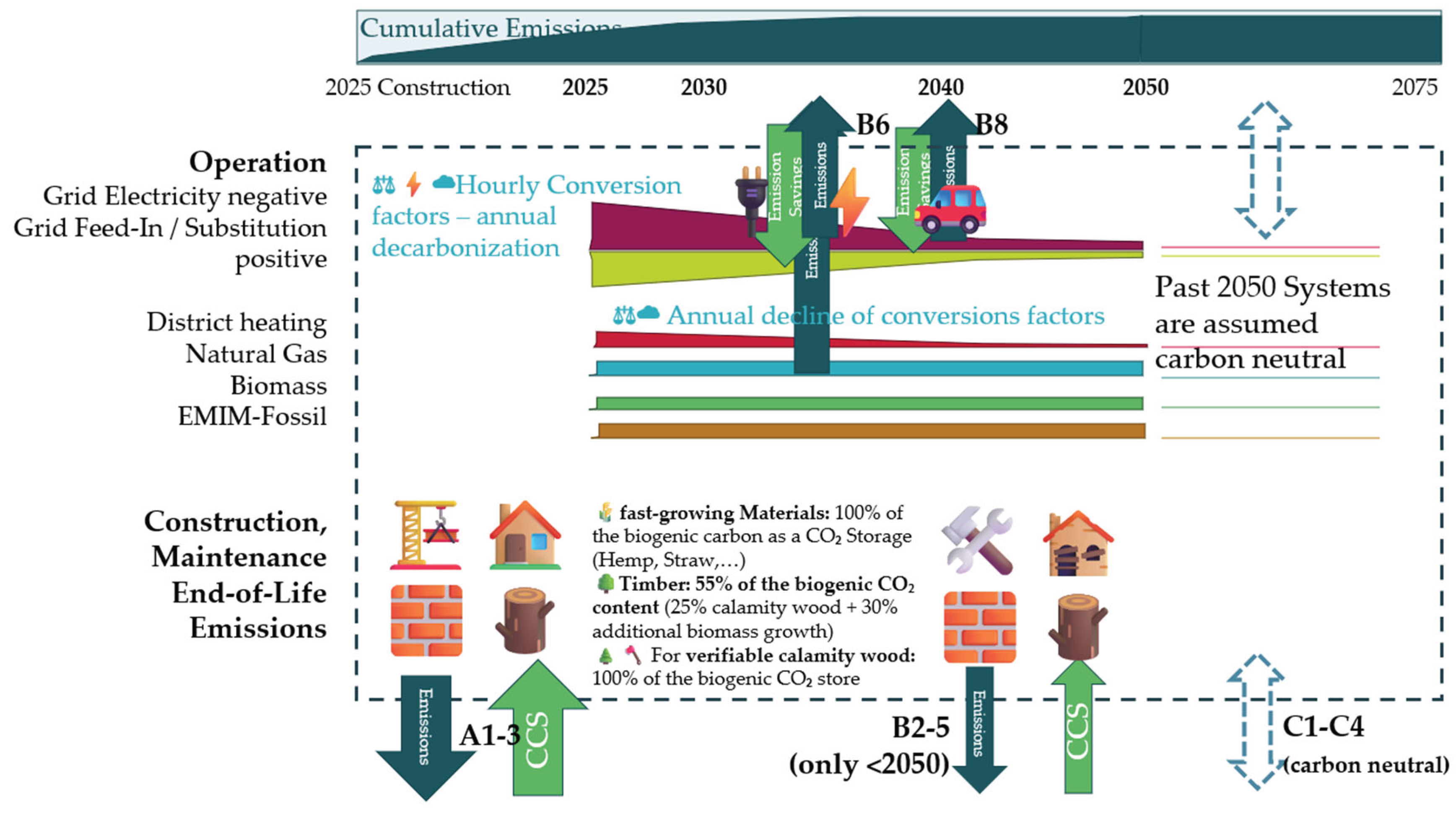
This section compares six baseline districts (D1–D6, configurations in Table 8) against the compliance framework using consistent project descriptors and harmonized KPIs. Lifecycle performance is summarized in Table 10 and Figure 7, Figure 8 and Figure 9: cumulative GHG per m² GFA is decomposed into A1–A3 (construction incl. TES + EMIM embodied), B-ops (time-resolved electricity and thermal operation), EMIM operation, and PV substitution credits (D2); we also report the primary energy (PE) balance. Compliance bands are shown at L3 = 320, L2 = 196, L1 = 72 kgCO₂e·m⁻²GFA.
Results are heterogeneous across use types and system choices. Relative to the L3 budget, the modeled GHG balances show: D1 +29.2, D2 −27.4, D3 −42.0, D4 −108.7, D5 +29.0, D6 +300.2 kgCO₂e m⁻² (overshoot positive; undershoot negative). PE balance passes in D1, D2, D4, D6 but not in D3, D5. District-level drivers:
Figure 5.
Baseline life cycle GHG balance by district. Cumulative emissions 2025–2075 per m² GFA, decomposed into A1–A3 (building, TES, and EMIM embodied), B-ops (building/TES with time-resolved grid factors), EMIM operation, and PV substitution credits (D2); CCS shown where applicable. Horizontal bands denote compliance thresholds (L3 = 320, L2 = 196, L1 = 72 kgCO₂e·m⁻²GFA).

D1 (greenfield, conventional): Non-compliant at L3 (+29.2). High A1–A3 intensity dominates; EMIM measures reduce operational mobility loads but cannot offset embodied peaks.
D2 (school campus): Benefits from the EMIM context (only commuting staff; high PV self-use + flexible charging), hybrid-eco materials achieving L3 compliance (−27.4) and a positive PE balance.
D3 (urban housing, DH): Meets L3 (−42.0) but fails PE (−47.7 kWhPE m⁻²·a). Lack of supply-side flexibility on DH limits net-positive operation despite acceptable GHG.
D4 (ecologic renovation + TABS/GSHP + mobility measures): Strongest performer across both metrics (−108.7; positive PE). Renovation and density factors reduce embodied intensity; mobility context halves residual EMIM; TABS/GSHP enable flexible, low-carbon operation.
D5 (conventional renovation, gas→DH): Switch to DH alone is insufficient for L3 (+29.0) and fails PE; Section 3.5 explores compliant variants (non-fossil TES + eco materials + flexibility).
D6 (low heat demand, high embodied/EMIM): Despite a positive PE balance, very high embodied and/or mobility-related loads lead to substantial L3 overshoot (+300.2).
Figure 6.
Primary energy balance by district. Demand (HVAC heat, electricity, mobility) and supply (PV self-use & export as grid substitution, energy-flexible operation, contextual factors). The zero line marks the positive PE balance requirement; DH without flexibility generally struggles to cross it, whereas GSHP+TABS and flexible operation perform better.
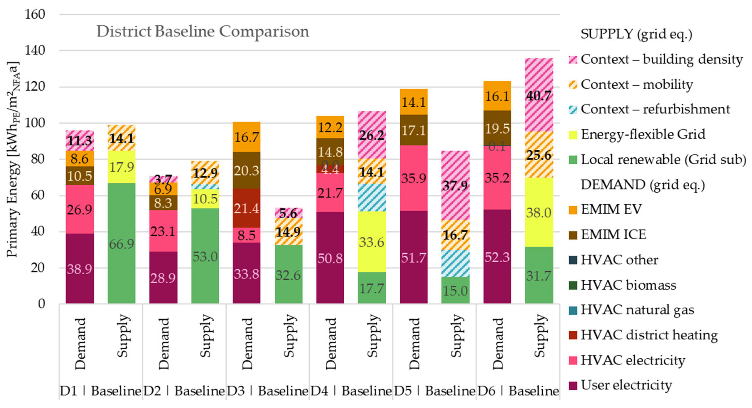
Figure 7.
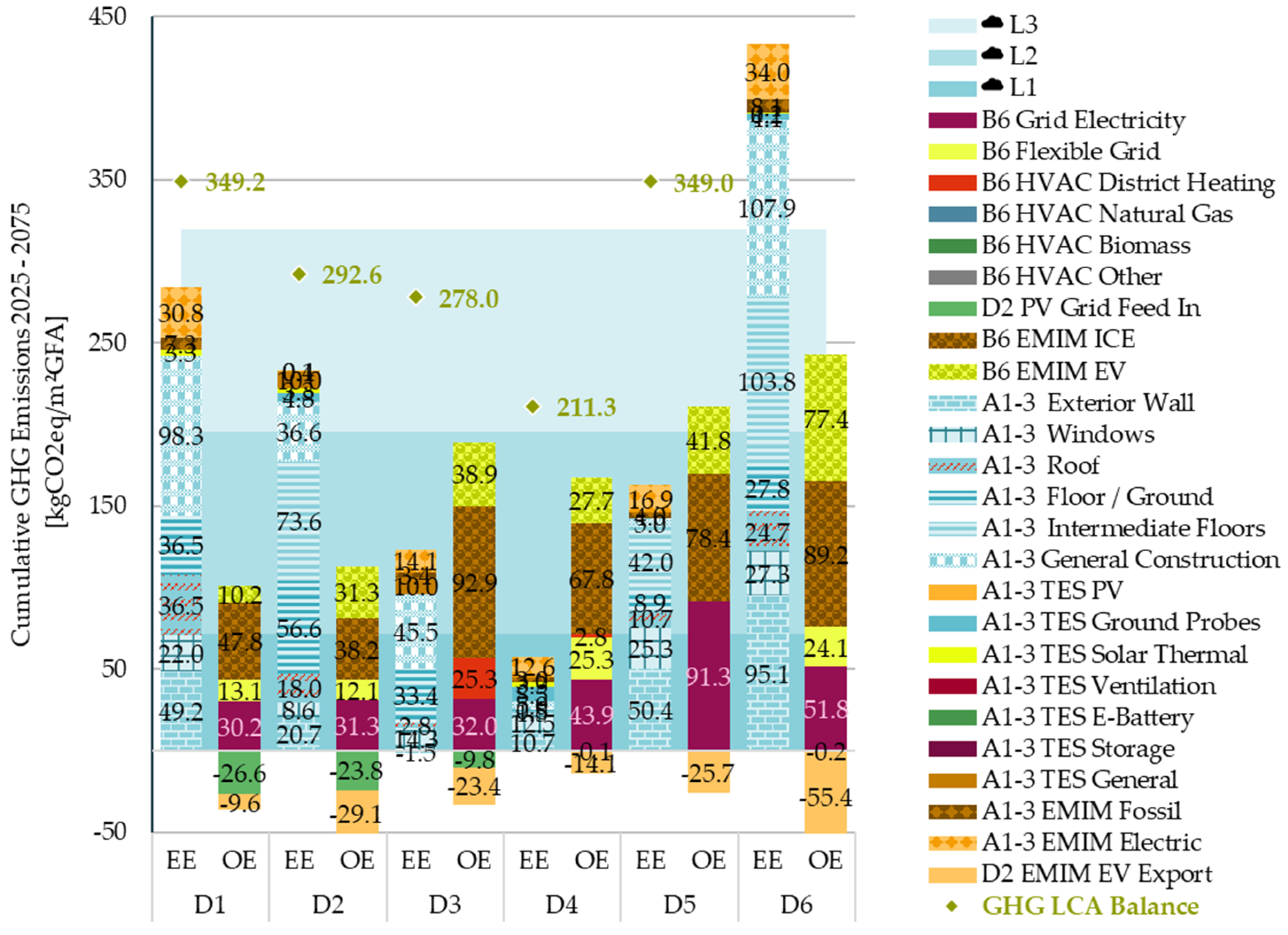
Cumulative GHG balance (2025–2075) with full LCA breakdown. For each district (D1–D6), the left bar (EE) shows embodied impacts (A1–A3, B2-B5) from construction and technical systems (TES, PV, batteries, ground probes) and embodied mobility. The right bar (OE) shows operational impacts (B6) from grid electricity and HVAC carriers (district heating, natural gas, biomass, other) plus EMIM (ICE/EV, B8.1-2) operation and flexible-grid effects; negative segments reflect avoided-grid D2 substitution (e.g., PV feed-in, EV other travel exports). Green diamonds indicate each district’s net LCA total, while shaded bands mark according compliance thresholds L3 = 320, L2 = 196, L1 = 72 kgCO₂e·m⁻²GFA. Positive stacks add emissions; negative stacks reduce the balance.
Figure 7.
Cumulative GHG balance (2025–2075) with full LCA breakdown. For each district (D1–D6), the left bar (EE) shows embodied impacts (A1–A3, B2-B5) from construction and technical systems (TES, PV, batteries, ground probes) and embodied mobility. The right bar (OE) shows operational impacts (B6) from grid electricity and HVAC carriers (district heating, natural gas, biomass, other) plus EMIM (ICE/EV, B8.1-2) operation and flexible-grid effects; negative segments reflect avoided-grid D2 substitution (e.g., PV feed-in, EV other travel exports). Green diamonds indicate each district’s net LCA total, while shaded bands mark according compliance thresholds L3 = 320, L2 = 196, L1 = 72 kgCO₂e·m⁻²GFA. Positive stacks add emissions; negative stacks reduce the balance.
3.2.1. Effects of PV TES Embodied Emission (Non-)Inclusion
As argued in Section 2.4.1, embodied emissions from PV systems are not part of this PED system boundary but instead nationally budgeted in the energy sector. Table 11 shows the omitted PV EE in contrast to the remaining balance: Especially for low-density districts that require a significantly positive PE-balance and PV export to offset their negative density context factor and for refurbishment projects with inherently low EE, PV EE can increase overall LCA emissions by more than 10% (assuming 1.16 t CO2e·kWp-1 incl. inverters and cabling).
3.3. Case Study District 3: Redevelopment of Urban Medium Density Residential District: Interplay of Embodied and Operational Emission Reduction Measures
The case study evaluates multiple redevelopment scenarios for an urban medium-density residential district (District 3). Variants differ in construction materials (fossil-intensive vs. ecological), PV system sizing (1×, 2.6×, 2×, 1.7×), mobility assumptions (70% EV, 100% EV, reduced traffic), and heating/DHW supply (district heating vs. ground-source heat pump). The main assessment criteria are the cumulative GHG balance (2025–2075) and the primary energy balance for PED compliance.
The results in Table 12, Figure 8 and Figure 9 show that all scenarios with ecological construction remain within the L3 compliance limit, while only the fossil construction variants exceed it. The combination of 2× PV oversizing with mobility measures (full electrification and reduced traffic) performs particularly well, even reaching the precautionary compliance limit for cumulative GHG emissions. This underlines the necessity of combining renewable supply expansion with systemic demand-side measures.
Figure 8.
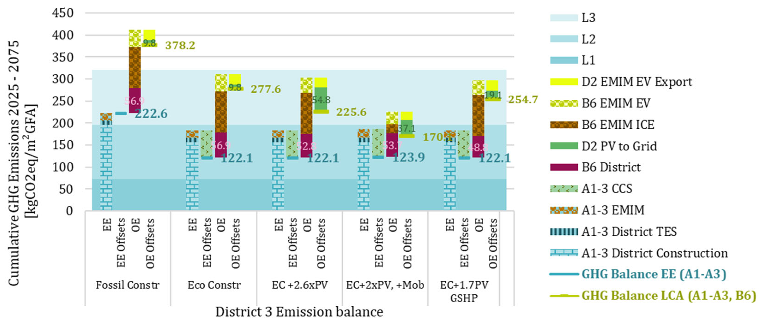
Cumulative GHG emissions (2025–2075) of district scenarios compared to compliance, precautionary, and Paris-compatible limits. Bars show embodied emissions (construction, technical systems, mobility), operational emissions, avoided emissions (grid feed-in), and carbon capture. Results highlight that fossil-based construction exceeds budget limits, whereas scenarios with extended PV and mobility measures approach or meet precautionary compliance thresholds.
Figure 8.
Cumulative GHG emissions (2025–2075) of district scenarios compared to compliance, precautionary, and Paris-compatible limits. Bars show embodied emissions (construction, technical systems, mobility), operational emissions, avoided emissions (grid feed-in), and carbon capture. Results highlight that fossil-based construction exceeds budget limits, whereas scenarios with extended PV and mobility measures approach or meet precautionary compliance thresholds.
At the same time, the assessment framework requires not only compliance with the finite GHG budget but also a positive primary energy balance. Here, the analysis reveals significant challenges: while PV oversizing improves operational balances, achieving a net-positive balance is difficult in configurations relying on district heating (DH) even when assuming renewable CHP-based supply with favorable emission factors. In contrast, scenarios with on-site GSHP systems combined with PV come closest to fulfilling both compliance criteria simultaneously, emphasizing the importance of coupling low-carbon construction materials with renewable-based, highly efficient supply systems.
3.4. Case Study District 4: Effect of Dynamic vs. Static Grid Emission Factors and Flexibility Signals
For District 4 we quantify how the temporal resolution and level of grid-GHG signals affect (i) total operational emissions from B6 electricity and EMIM-EV charging, and (ii) the average effective grid-intensity seen by the project. We compare monthly, building-code style factors (OIB ‘19/’23, currently in effect) with hourly, live-tracking based factors for the same vintages. We first test flexibility via TABS GS HP heating (+3K) and cooling (-2K), then in combination with building battery (BESS) sized = PV installed capacity (kWp) and EV bidirectional charging (V2B, down to 50% SoCRES). Loads & controls held constant: Building demand, PV generation, HVAC control set-points (22°C heating, 25°C cooling), occupancy, and the EMIM travel demand are fixed across scenarios. Only the GHG emission factors and flexibility signals vary:
GHG Emission factors.
- Monthly and annual factors (2019 M, 2023 M, 2019 A) Twelve constant monthly values per vintage or a constant annual value as shown in Figure 10.
- Hourly factors (2023 H). 8760 time steps based on historic live tracking; annual means match the corresponding OIB vintage 2023 (see Figure 10)
Flexibility Signals
- Wind Peaks (for 2020, above 50% nominal Power)
- GHG Emission rolling averages: signal if current GHG EF(t) is y% below Rolling Average (x hour future window) (x ∈ {+24,+48,+72}, y ∈{5%,10%})
Table 13.
Scenario definition for case study District 4.
| Scenario | Grid Emission (Figure 10) | Flexibility Signal | Flexibility Option(s) |
| 19 M | 2019 M | Wind Peaks >50%Pnom | TABS |
| 19 A | 2019 A | Wind Peaks >50%Pnom | TABS |
| 23 M (Baseline) | 2023 M | Wind Peaks >50%Pnom | TABS |
| 23H 24-5 | 2023 H | RA x=24, y= 5% | TABS |
| 23H 48-5 | 2023 H | RA x=48, y= 5% | TABS |
| 23H 48-10 | 2023 H | RA x=48, y=10% | TABS |
| 23H 72-10 | 2023 H | RA x=72, y=10% | TABS |
| 23H 48-10 BESS | 2023 H | RA x=48, y= 10% | TABS + BESS |
| 23H 48-10 BESS V2B | 2023 H | RA x=48, y= 10% | TABS + BESS + V2B |
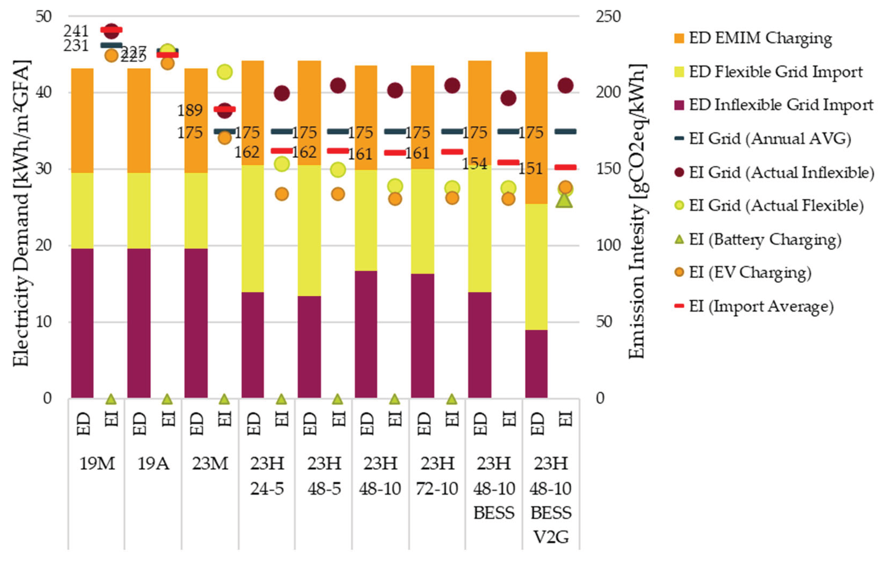
This use case highlights why hourly emission accounting is essential. With monthly factors, the import-weighted average EI is higher than the annual grid average (≈241→231 gCO₂e·kWh-1 for 2019 and 189→175 for 2023) because districts typically import in winter (carbon-intensive) and export PV in summer (cleaner). Annual bookkeeping would therefore “hide” the winter penalty; capturing it is critical—but without flexible dispatch comes at the cost of higher emissions – arguably as it should be.
Switching to hourly factors and applying rolling-average GHG signals enables flexible loads to target low-EI hours. In our runs the import-weighted EI drops from ~189 gCO₂e·kWh-1 (2023 monthly) to ~160 gCO₂e·kWh-1 with hourly signaling alone, and to ~150 gCO₂e·kWh-1 when BESS and V2B are added. The grid EI for inflexible demand remains comparatively high (≈200 gCO₂e·kWh-1) because it is drawn during scarcity events when storage is depleted—another effect only visible with hourly accounting.
The results also show that flexibility generally slightly increases total electricity demand (round-trip and conversion losses; more charging activity), but because a larger share becomes flexible and is shifted to low-EI hours, net GHG emissions fall (our KPI), and the average effective EI of imports/charging (second KPI) improves materially. In short: hourly signals + storage/V2B make compliance harder to “paper over” yet provide a real, quantifiable pathway to lower life-cycle emissions.
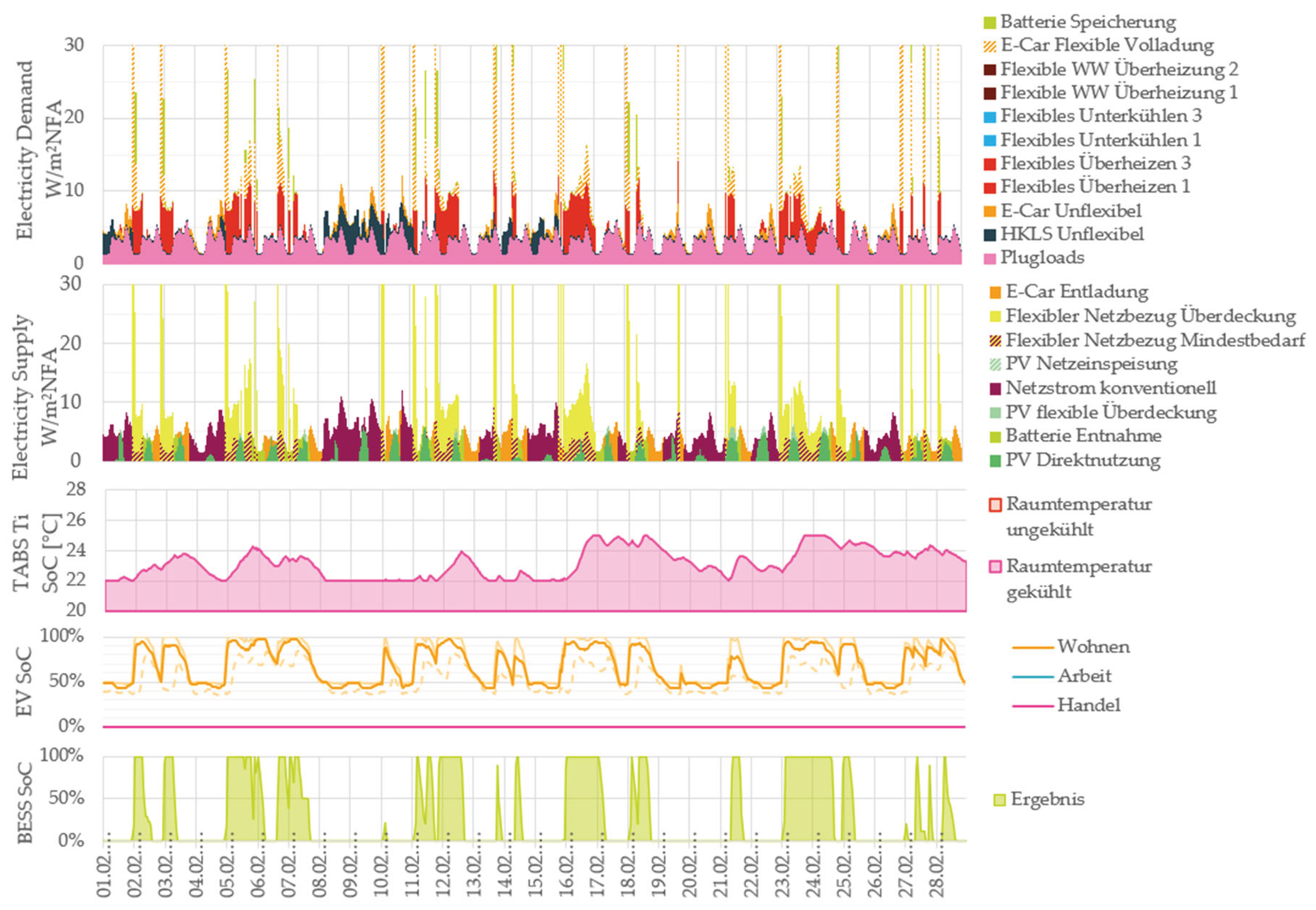
Figure A1 shows how energy demand, supplies and flexibility options are dispatched on an hourly basis for Scenario “23H 48-10 BESS V2G”.
Table 14.
Operational life cycle Emissions (OE), PE Balance, Imported Electricity (ED), relative differences to the Baseline (and Emission Intensities (AVG=Annual Grid Average, Actual = Actual district import average).
Table 14.
Operational life cycle Emissions (OE), PE Balance, Imported Electricity (ED), relative differences to the Baseline (and Emission Intensities (AVG=Annual Grid Average, Actual = Actual district import average).
| Scenario |
OE (B6-D2) |
∆BL % |
PE Balance kWh·m⁻²·a⁻¹ |
ED kWh·m⁻²·a⁻¹ |
∆BL % |
EIGrid gCO₂e·kWh-1 |
EIdistrict gCO₂e·kWh-1 |
∆EI/EIGrid % |
| [%]19M | 175.4 | +14.4 | +6.3 | 43.2 | 0.0 | 231 | 241.0 | +4.2 |
| 19A | 167.3 | +9.1 | +6.6 | 43.2 | 0.0 | 227 | 224.6 | -1.1 |
| 23M (Baseline) | 153.3 | - | +2.8 | 43.2 | - | 175 | 188.9 | +7.4 |
| 23H 24-5 | 141.3 | -7.8 | +22.2 | 44.2 | +2.3 | 175 | 162.1 | -8.0 |
| 23H 48-5 | 141.2 | -7.9 | +22.5 | 44.2 | +2.3 | 175 | 161.9 | -8.1 |
| 23H 48-10 | 139.4 | -9.0 | +14.4 | 43.6 | +0.9 | 175 | 160.6 | -9.0 |
| 23H 72-10 | 139.8 | -8.8 | +14.7 | 43.6 | +1.0 | 175 | 161.1 | -8.6 |
| 23H 48-10 BESS | 137.3 | -10.4 | +19.3 | 44.2 | +2.3 | 175 | 154.2 | -13.5 |
| 23H 48-10 BESS V2G | 137.9 | -10.0 | +25.6 | 45.4 | +5.1 | 175 | 151.3 | -15.7 |
Figure 11.
Temporal GHG signals and flexibility for District 4. Stacked bars (left axis) show annual electricity demand split into inflexible grid import, flexible grid import, and EMIM EV charging. Markers (right axis) report effective emission intensities (EI) for imports and charging. Scenarios progress from monthly factors (19M, 19A, 23M) to hourly factors with rolling-average signals (23H 24–5, 48–5, 72–10, 48–10) and three flexibility options (TABS – all, BESS = PV-sized battery; BESS V2G = battery plus EV V2B). The dashed blue line is the annual-average grid EI; filled markers show actual EI of inflexible imports, flexible imports, EV charging, and battery charging; the red bar give the realized import-weighted average EI.
3.5. Case Study District 5: Mobility and Renovation Sensitivity
The case study illustrates the cumulative GHG emissions of an identical district configuration (70 multistory buildings) across different spatial contexts, with mobility-related emissions added. It shows that EMIM can dominate total emissions, even in not-decarbonized districts such as this gas-heated example. We investigate District 5 with a factorial scenario set spanning four drivers of mobility-related impacts and their interaction with energy supply and envelope choices as shown in Table 15. Figure 12 shows the mileage differentiation of [52] used in this framework as described in [14,53,54].
District location and accessibility to public transport strongly influence travel demand, resulting in average annual personal motorized mileage ranging from about 4,000 km in metropolitan contexts to 11,831 km in rural areas with high commute and low public transport availability (Region 24). Consequently, cumulative district emissions shown in Figure 13 vary widely — from about 740 kgCO₂e·m⁻²GFA in the fossil-fuel-based, rural commuter case down to 27 kgCO₂e·m⁻²GFA in the fully electrified, metropolitan case with high shares of alternative transport modes. This can further be reduced by active mobility measures in the district such as bike and car sharing opportunities to reduce the total annual mileage by EMIM. This shows that L3 compliance (320 kgCO₂e·m⁻²GFA over 2025–2075) is possible in all locations, but complete electrification of vehicles until 2050 (averaging an EV share of 50%+ from 2025-2075) is essential. Measures to shift the modal split away from EMIM to public transport, pedestrian and bikes can help also but may not be sufficient by themselves.
3.5.1. Impacts of Refurbishment
Table 16 reports KPIs, and Figure 14 and Figure 15 visualize composition for seven refurbishment options under the metropolitan mobility case with 70% EV: Unrenovated fossil gas (Gas SQ) violates all limits (~753 kgCO₂e·m⁻²GFA). Switch to District heating without refurbishment (DH SQ) reaches GHG compliance (~196, L2) but without efficiency measures fails the PED/primary-energy target. Conventional renovation is not reliably compliant (DH Conv-Reno ~334; GSHP Conv-Reno ~360), whereas ecologic renovations reduce A1–A3 and are robust (DH Eco-Reno ~246; GSHP Eco-Reno ~245). GSHP Conv-Flex remains within L3 (~293) thanks to higher avoided-grid credits and reduced operation, and—critically—enables a positive primary-energy balance, illustrating that a climate-neutral PED is difficult but feasible when non-fossil TES is combined with flexibility even for an arguable worst case scenario of dense urban areas with little potential for energy efficiency and local renewable energy (Roof PV installations are required on all roofs up to conservative estimates).
3.5.2. Sensitivity to Location and Renovation
Figure 16 plots embodied emissions on the x-axis and operational emissions (including EMIM) on the y-axis for five location types (rural-1, rural-2, suburban, urban, metropolitan). Blue diagonals mark the cumulative-budget limits L3 (320), L2 (196), and L1 (72) kgCO₂e·m⁻²GFA to 2050. Marker fill indicates EV share (5–100%), outlines the thermal energy system (blue = gas, red = district heating, yellow = GSHP), and shapes the construction choice (square = no renovation, triangle = code-compliant renovation, circle = ecological renovation).
In the “no renovation” cases (top row), points cluster far left—reflecting very low embodied emissions—but sit high on the y-axis because the envelope is unchanged. Where district heating is available, several variants fall below L3 on GHG alone; gas heating generally breaches L3, particularly in rural settings where mobility dominates. Raising the EV share pushes points downward across all locations yet seldom achieves L2 or L1 without fabric measures.
With renovation (bottom row), points move right as embodied emissions rise, while y-values drop markedly—most strongly when GS HPs are combined with high EV penetration. In suburban, urban, and metropolitan contexts, many renovated variants approach or meet L2, and a few edge toward L1 when ecological materials are used. Rural districts remain the most challenging because mobility keeps operational totals elevated.
Overall, if the sole objective were cumulative GHG-budget compliance, a “do-nothing fabric” strategy paired with low-carbon district heating could pass L3. However, it fails PED/primary-energy goals: without efficiency upgrades, primary energy demand remains high, and the district cannot achieve a positive PE balance. Meeting both the climate-budget and PED criteria requires renovation (preferably but not necessarily ecological), electrified heat (GSHP or very low-carbon CHP DH), and high EV shares to reduce operational and mobility-related emissions simultaneously.
3.6. Case Study District 6: Differences in Construction Practice and Materials
This case study illustrates the application of the simplified biogenic carbon accounting method to the planned green-field development District 6 and highlights that construction choice dominates D6’s life-cycle GHG outcome (Table 17 and Figure 17):
The Baseline structural design of the project is based on conventional building practice with a reinforced concrete framework, thermal insulation using expanded polystyrene (EPS), with mineral wool in areas requiring enhanced fire resistance. The district benefits from high urban density and mixed-use zoning, supported by excellent public transport accessibility. As a result, the underground parking facility can be designed with a single basement level and a reduced parking ratio, further limiting construction-related GHG emissions. The high building compactness enables comparatively low EE during the construction phase.
Despite these advantages, the total CO₂-equivalent emissions from both construction and operation exceed the allocated climate neutrality budget. Even with relatively low operational EI for building use and EMIM, the project surpasses the allowable threshold by more than 75% over the 50-year assessment period.
Scenario “Eco Skeleton” introduces a more ecologically ambitious system, featuring a reduced structural frame with timber elements and mineral wool insulation. Although this scenario represents an improvement over the traditional concrete structure, the CO₂ emissions remain 30% above the maximum compliance limit due to the use of steel-reinforced concrete in the structural elements.
Scenario “Mixed-Use CLT” incorporates a combination of concrete and cross-laminated timber (CLT). This mixed approach, including wood-concrete composite decks and CLT for upper floors, leads to a significant reduction in emissions compared to the first two scenarios, while still maintaining structural integrity and near L3 compliance.
Scenario "Max-Eco" represents the most ecologically advanced scenario, pushing the boundaries of climate-neutral construction. It utilizes CLT, straw insulation, wood-fiber insulation, and clay boards, minimizing the use of concrete to only necessary structural components. This results in the lowest emissions, making it the most sustainable option among the four, though it involves compromises, such as relaxing some fire protection regulations. An alternative pathway to compliance would involve further reducing operational and mobility-related emissions. For example:
- Increasing the installed PV Capacity,
- Raising the share of electric vehicles in the mobility mix,
- Implementing more ambitious ecological construction measures (e.g., low-carbon materials).
4. Discussion
The proposed climate neutrality assessment framework for PEDs aims to bridge the gap between research-grade, high-resolution analysis and practical, policy-aligned application. By defining clear system boundaries, integrating dynamic emission factors for multiple energy carriers, and embedding the assessment in a finite CO₂ budget, it offers a robust yet operationally feasible tool for evaluating district-level climate performance. The framework’s treatment of local PV—crediting both self-consumption and grid substitution—along with its differentiated decarbonization pathways, supports both design optimization and strategic policymaking. The following subsections discuss the methodological implications, applicability and limitations, and policy relevance of this approach.
4.1. Methodological Implications
Positive Energy Districts are framed here as vehicles for verifiable climate neutrality. The assessment boundary is refined to include operational emissions, EMIM, and selected embodied emissions, while transparently excluding categories allocated to other sectors in the national carbon budget (e.g., PV embodied impacts; end-of-life beyond 2050). This departs from conventional LCA allocations (e.g., attributing the embodied impacts of generation assets to the consuming district) and makes explicit how sectoral budgets are coupled.
Temporal resolution is central. Hourly conversion factors capture the variability of electricity and heat mixes and enable the evaluation of demand shifting and storage. For declarations, monthly factors aligned with Austrian code are used to ensure comparability and administrative simplicity. Carrier-specific decarbonization pathways are differentiated: electricity and district heating follow a declining trajectory to (near) zero by 2050, while gas, biomass, and other fossil carriers retain constant intensities over the horizon. Using static, time-invariant factors would implicitly assume society fails to decarbonize by 2050; the framework instead embeds the policy trajectory, after which the budget is exhausted and historic LCA conventions become less informative.
Local PV is treated on a system basis. Onsite generation offsets grid consumption at the time-varying CO₂ intensity of the avoided imports; exports are credited for grid substitution (D2), recognizing their contribution to system decarbonization. This contrasts with net-zero approaches that ignore export credits, and it materially affects both design optimization and policy interpretation in PED contexts.
Separating measurement effects from control effects is important. Hourly factors expose seasonal import–export asymmetries that annual bookkeeping masks, while dynamic flexibility signals (wind-peak-events, GHG rolling-averages, price signals, etc) guide storage, charging, and thermal shifting to lower import-weighted intensities. Declarations remain simple and comparable, while design and operation can be assessed with rigor and temporal fidelity. Crucially, it prevents projects over-crediting flexibility measures and allows PED compliance to be evaluated transparently against both carbon budgets and energy balance criteria. This clarity improves interpretation but means results are sensitive to the chosen signal and available assets (BESS, TABS, V2B) – an interconnection which would benefit from further research so it can be better designed for. Overall, the approach is auditable and declaration-ready, but data localization and policy-trajectory uncertainty remain the main limits.
A finite-budget perspective tightens alignment with Paris-compatible trajectories. Front-loaded embodied emissions cannot be “repaid” later without crowding out the remaining budget, so low-carbon construction becomes a first-order design variable alongside operational efficiency and mobility measures. Annualized KPIs can conceal this timing problem by spreading construction impacts evenly over service life; the budget lens restores the correct climate signal by tracking accumulation and scarcity over time.
4.2. Applicability and Limitations
Applicability. The framework is applicable to a wide range of PED sizes, usages and typologies, from small urban districts to large-scale developments, both for renovation and green-field developments. Its adaptability stems from the modular definition of system boundaries, context factors and the flexibility in selecting conversion factors based on data availability and assessment purpose. In practice, high-resolution operation and mobility inputs are not always available; calibrated defaults allow use at early stages but reduce fidelity.
Changing Assumptions. While the assumption of zero emission processes after 2050 streamlines the assessment, these assumptions may not hold if decarbonization timelines shift. Moreover, the exclusion of certain embodied emissions—particularly those for PV systems—relies on the integrity of the national budget allocation methodology.
Regulatory alignment is strong with the Austrian building code, but deviations from international standards, particularly EN 15978, may affect acceptance in cross-border contexts. The focus on a fixed 2050 endpoint aligns with current climate targets but may require revision in the event of accelerated or delayed policy timelines.
Transferability beyond Austria is straightforward in method but requires localizing decarbonization pathways, carrier factors, mobility contexts, and code constraints (e.g., tall-timber fire rules, façade-PV allowances). The framework embeds a Paris-aligned trajectory to 2050 and assumes (near-)zero-carbon electricity/DH thereafter; if national timelines diverge, factors and budgets must be re-parametrized. Excluding PV embodied impacts at project level relies on coherent sectoral accounting; where this is not in place, a documented alternative (including PV embodied with a compensating sectoral adjustment) may be warranted.
4.3. Policy Implications
Adoption as Declaration. The presented framework underpins a national labeling/declaration scheme in Austria (“klimaaktiv” [27,55]), providing consistent, comparable verification and a practical bridge between research-grade assessment and regulatory adoption. With localized factors, it can harmonize with emerging EU instruments (EPBD revisions, taxonomy), supporting broader uptake while maintaining the rigor needed for credible climate-neutral PED claims.
Adoption in Practice. The framework enables municipalities and developers to test whether districts are on Paris-compatible paths by combining two KPIs—a finite cumulative GHG budget and a positive primary-energy balance—within transparent boundaries that include user-driven mobility. Moving from annual KPIs to a 25-year cumulative budget refocuses decisions on near-term embodied and operational peaks, closing a key blind spot in conventional PED assessments. Authorities can request framework compliance as part of development agreements and contracts, or set concrete, verifiable targets (e.g., max embodied GHG per m², minimum flexible PV/BESS/V2B capacity, DH decarbonization milestones) and align procurement, permitting, and incentives accordingly. Separating measurement (hourly EF) from control (flexibility signals) also gives a policy lever to reward time-aware operation rather than nominal annual surpluses. This should further be aligned with national adoption plans for Smart Readiness Indicators (SRI).
5. Conclusions
We present a declaration-ready framework for assessing climate-neutral Positive Energy Districts (PEDs) that combines finite CO₂ budgets, explicit system boundaries, and dynamic emission factors. It reconciles research-grade accuracy (hourly CO₂ intensity and differentiated decarbonization paths) with policy usability. Core Elements:
- Two KPIs with targets: (1) cumulative GHG budget to 2050 and (2) annual primary-energy balance for declaring PED status (with/without mobility).
- LCA scope: unified accounting of construction, operation, and EMIM mobility (including embodied construction, maintenance, end-of-life) over the next 25 years within a single CO₂ budget.
- Alignment with national sector targets: PV embodied impacts remain in the energy sector and are excluded at project level; non-EMIM travel modes (PT, walking, cycling) remain in the transport sector. PV exports are credited with time matching.
- Time-resolved emissions and pathways: hourly (or monthly) grid factors; distinct decarbonization trajectories for electricity and renewables; constant intensities for gas/biomass/other fossil carriers (with DH inheriting its supply mix).
Applied across diverse Austrian districts, the framework is practical, transparent, and auditable—supporting credible compliance pathways and ready adoption in labeling/declaration schemes.
Design implications. Case study applications show that even highly efficient PED designs can exceed the available CO₂ budget unless embodied emissions are minimized (through low-carbon/biogenic options, lean structures), renewable energy and flexibility contributions are maximized (through flexible dispatch with BESS/V2B/TABS), and operational emissions from user-driven mobility are effectively reduced (by electrification and demand reduction).
Limitations. Transferability depends on localized data; early-stage inputs can be noisy; building codes constrain options (e.g., fire rules for tall timber, façade-PV); and policy/decarbonization trajectories remain a source of uncertainty.
Next steps.
- Link to dynamic LCA databases to strengthen embodied-emissions estimates.
- Adapt to diverse regulatory contexts and add uncertainty analysis for pathways.
- Automate compliance checks and embed the workflow in planning regulations and municipal decision processes.
Author Contributions
Conceptualization, S.S.; methodology, S.S and T.Z..; software, S.S., P.K.; validation, T.Z.., formal analysis, S.S. and T.Z..; investigation, S.S., R.D.; resources, S.S., T.Z. and R.D.; data curation, S.S., R.D., M.S. and P.K.; writing—original draft preparation, S.S.; writing—review and editing, T.Z., R.D., J.B.; visualization, S.S.; supervision, J.B.; All authors have read and agreed to the published version of the manuscript.
Funding
This research was funded by the City of Vienna MA23, grant number 35-2 “Competence Team for teaching Climate-Fit City Renovation”
Data Availability Statement
Data is available at the GitHub repository [33] under https://github.com/simonschaluppe/peexcel/tree/master/data/publications/2025-Declaration-Ready-Climate-Neutral-PEDs
Acknowledgments
During the preparation of this manuscript/study, the author(s) used ChatGPT v5 for the purposes of text formulation and review. The authors have reviewed and edited the output and take full responsibility for the content of this publication.
Conflicts of Interest
The authors declare no conflicts of interest.
Abbreviations
The following abbreviations are used in this manuscript:
| ACH | Air Changes per Hour |
| AS HP | Air Source Heat Pump (Air to Water) |
| BESS | Battery Energy Storage System |
| CLT | Cross-laminated Timber |
| COP | Coefficient of Performance |
| DH | District Heating |
| DHW | Domestic Hot Water |
| EI | Emission Intensity |
| EMIM | Everyday motorized individual Mobility |
| EV | Electric Vehicle |
| FSI | Floor space index |
| GHG | Greenhouse Gas |
| GFA | Gross Floor Area |
| GS HP | Ground source Heat pump (boreholes) |
| HVAC | Heating, ventilation, air conditioning and DHW |
| ICE | Internal combustion engine (vehicle) |
| LCA | Life Cycle Assessment |
| NFA | Net Floor Area |
| PAX | Persons approximate |
| PEF | Primary Energy Factor |
| PE tot | Total Primary Energy |
| PE nre | Non-renewable Primary Energy |
| PE re | Renewable Primary Energy |
| PED | Positive Energy District |
| PV | Photovoltaics / Photovoltaic System |
| TES | Technical Building Energy Systems |
| TSD | Time Series Data |
| V2G | Vehicle to Grid |
| V2B | Vehicle to Building |
Appendix A
Figure A1.
Hourly Flexibility Operation in February Scenario “23H 48-10 BESS V2G” showing Electricity demands (Top), Electricity supplies (below, note the flexible grid charging in lime and V2B in orange), Storage SoCs (TABS indoor Temperature), EV Battery SoC (dashed =avg offsite SoC, solid=avg SoC, thin solid = avg SoC onsite) and Battery Energy system SoC.
References
- United Nations Framework Convention on Climate Change Paris Agreement 2015.
- IPCC Climate Change 2021: The Physical Science Basis. Contribution of Working Group I to the Sixth Assessment Report of the Intergovernmental Panel on Climate Change 2021.
- IPCC, Core Writing Team, H. Lee and J. Romero (eds.) Climate Change 2023: Synthesis Report. Contribution of Working Groups I, II and III to the Sixth Assessment Report of the Intergovernmental Panel on Climate Change; IPCC: Geneva, Switzerland, 2023. [Google Scholar]
- Climate Change 2022 - Mitigation of Climate Change: Working Group III Contribution to the Sixth Assessment Report of the Intergovernmental Panel on Climate Change; Intergovernmental Panel on Climate Change (IPCC), Ed. ; Cambridge University Press: Cambridge, 2023.
- Rogelj, J.; Shindell, D.; Jiang, K.; Fifita, S.; Forster, P.; Ginzburg, V.; Handa, C.; Kheshgi, H.; Kobayashi, S.; Kriegler, E.; et al. Mitigation Pathways Compatible with 1.5°C in the Context of Sustainable Development. Special Report on Global Warming of 1.5°C, IPCC 2018, 93–174. [Google Scholar] [CrossRef]
- IEA Net Zero by 2050 - A Roadmap for the Global Energy Sector; 2021; p. 224;
- Röck, M.; Ruschi Mendes Saade, M.; Balouktsi, M.; Rasmussen, F.N.; Birgisdottir, H.; Frischknecht, R.; Habert, G.; Lützkendorf, T.; Passer, A. Embodied GHG Emissions of Buildings – The Hidden Challenge for Effective Climate Change Mitigation. Applied Energy 2020, 230, 115–124. [Google Scholar] [CrossRef]
- JPI Urban Europe / SET Plan Action 3.2. White Paper on PED Reference Framework for Positive Energy Districts and Neighbourhood; JPI Urban Europe: Vienna, Austria, 2020. [Google Scholar]
- European Commission. Joint Research Centre. Enabling Positive Energy Districts across Europe: Energy Efficiency Couples Renewable Energy.; Publications Office: LU, 2020. [Google Scholar]
- European Commission 100 Climate-Neutral Cities by 2030 – by and for the Citizens: The Mission 2021.
- Lindholm, O.; Rehman, H. ur; Reda, F. Positioning Positive Energy Districts in European Cities. Buildings 2021, 11, 19. [Google Scholar] [CrossRef]
- Häkkinen, T.; Kuittinen, M.; Ruuska, A.; Jung, N. Reducing Embodied Carbon during the Design Process of Buildings. Journal of Building Engineering 2015, 4, 1–13. [Google Scholar] [CrossRef]
- Fawcett, T. Personal Carbon Trading: A Policy Ahead of Its Time? Energy Policy 2010, 38, 6868–6876. [Google Scholar] [CrossRef]
- Schneider, S.; Zelger, T.; Sengl, D.; Baptista, J. A Quantitative Positive Energy District Definition with Contextual Targets. Buildings 2023, 13, 1210. [Google Scholar] [CrossRef]
- Albert-Seifried, V.; Murauskaite, L.; Massa, G.; Aelenei, L.; Baer, D.; Krangsås, S.G.; Alpagut, B.; Mutule, A.; Pokorny, N.; Vandevyvere, H. Definitions of Positive Energy Districts: A Review of the Status Quo and Challenges. Sustainability in Energy and Buildings 2021 2022, 493–506. [Google Scholar]
- Steininger, K.W.; Meyer, L.; Nabernegg, S.; Kirchengast, G. Sectoral Carbon Budgets as an Evaluation Framework for the Built Environment. Buildings and Cities 2020, 1, 337–360. [Google Scholar] [CrossRef]
- Steininger, K.W.; Williges, K.; Meyer, L.H.; Maczek, F.; Riahi, K. Sharing the Effort of the European Green Deal among Countries. Nat Commun 2022, 13, 3673. [Google Scholar] [CrossRef] [PubMed]
- Habert, G.; Röck, M.; Steininger, K.; Lupísek, A.; Birgisdottir, H.; Desing, H.; Chandrakumar, C.; Pittau, F.; Passer, A.; Rovers, R.; et al. Carbon Budgets for Buildings: Harmonising Temporal, Spatial and Sectoral Dimensions. Buildings and Cities 2020, 1, 429–452. [Google Scholar] [CrossRef]
- European Committee for Standardization (CEN) CEN – European Committee for Standardization. prEN 15978:2024 — Sustainability of Construction Works – Assessment of Environmental Performance of Buildings – Requirements and Guidance, 2024.
- Cabeza, L.F.; Rincón, L.; Vilariño, M.V.; Pérez, G.; Castell, A. Life Cycle Assessment (LCA) and Life Cycle Energy Analysis (LCEA) of Buildings and the Building Sector: A Review. Renewable and Sustainable Energy Reviews 2014, 29, 394–416. [Google Scholar] [CrossRef]
- Mastrucci, A.; Marvuglia, A.; Leopold, U.; Benetto, E. Life Cycle Assessment of Building Stocks from Urban to Transnational Scales: A Review. Renewable and Sustainable Energy Reviews 2017, 74, 316–332. [Google Scholar] [CrossRef]
- Planetary Boundaries Assessment of Deep Decarbonisation Options for Building Heating in the European Union | Elsevier Enhanced Reader Available online:. Available online: https://reader.elsevier.com/reader/sd/pii/S0196890422013802?token=8CD397B53B87420B82FC9F1BFFFA6317A5F493CCCAB3825A79CA79362CDDF99BF3DFEE137533D71D012517B9706C6E11&originRegion=eu-west-1&originCreation=20230206090422 (accessed on 6 February 2023).
- Umweltbundesamt Austria National Energy and Climate Plan (NEKP) – Hourly CO₂ Intensities 2023.
- Pehl, M.; Arvesen, A.; Humpenöder, F.; Popp, A.; Hertwich, E.G.; Luderer, G. Understanding Future Emissions from Low-Carbon Power Systems by Integration of Life-Cycle Assessment and Integrated Energy Modelling. Nature Energy 2017, 2, 939–945. [Google Scholar] [CrossRef]
- IEA CO2 Emissions in 2023; Paris, 2024.
- Schneider, S.; Drexel, R.; Zelger, T.; Baptista, J. PEExcel: A Fast One-Stop-Shop Assessment and Simulation Framework for Positive Energy Districts.; IBPSA-Germany and Austria, 2024; Vol. 10, pp. 80–88.
- Stadt-Quartiere, Klimaaktiv Available online:. Available online: https://www.klimaaktiv.at/erneuerbare/erneuerbarewaerme/stadt-quartiere.html (accessed on 19 August 2024).
- Schneider, S.; Drexel, R.; Frech, C. Klimaneutrales Alliiertenviertel-2025-Wien - Open Government Data Austria, 2025.
- Schöfmann, P.; Zelger, T.; Bartlmä, N.; Schneider, S.; Leibold, J.; Bell, D. Zukunftsquartier - Weg zum Plus-Energie-Quartier in Wien; Berichte aus Energie- und Umweltforschung; Austrian Research Promotion Agency: Vienna, 2020. [Google Scholar]
- Schöfmann, P.; Forstinger, V.; Zelger, T.; Schneider, S.; Leibold, J.; Bell, D.; Schindler, M.; Mlinaric, I.; Hackl, L.; Wimmer, F.; et al. Zukunftsquartier 2. 2022. [Google Scholar]
- Schneider, S.; Zelger, T.; Kerschbaum, E.; Drexel, R.; Bell, D.; Goudarzi, S.; Paráda, E.; Schneider, U.; Berger, M.; Bucek, F.; et al. 2022.
- Schneider, S. 2023.
- Simon Schneider PED Assessment Framework Available online:. Available online: https://github.com/simonschaluppe/peexcel (accessed on 21 August 2025).
- Smith, S.M.; Geden, O.; Minx, J.C.; Nemet, G.F.; Gidden, M.; Lamb, W.F.; Powis, C. The State of Carbon Dioxide Removal Report 2023.
- Aspern Klimafit 2.
- Drexel, C.; Mörth, W. Zwei Grad. Eine Tonne. - Wie wir das Klimaziel erreichen und damit die Welt verändern.; Laible Verlagsprojekte: Allensbach, 2018; ISBN 978-3-200-05606-0. [Google Scholar]
- Statistics Austria STATatlas Available online:. Available online: https://www.statistik.at/atlas/?theme=6 (accessed on 6 June 2022).
- Thomas Zelger; Jens Leibold; Simon Schneider; Flora Bachleitner; Jasmin Helnwein; Peter Holzer; David Stuckey; Annekatrin Koch; Bettina Doser; Christof Drexel; et al. Aspern Klimafit 2.0, 2024.
- Amann, W.; Goers, S.; Komendantova, N.; Oberhuber, A. Kapazitätsanpassung der Bauwirtschaft für eine erhöhte Sanierungsrate; Berichte aus Energie- und Umweltforschung; Wien, 2021.
- Österreichisches Normungsinstitut Austrian Standards International. Nachhaltigkeit von Bauwerken – Umweltdeklarationen für Bauprodukte – Grundregeln für die Produktkategorie Bauprodukte (ÖNORM EN 15804).
- Oekoindex OI3 - IBO - Österreichisches Institut Für Bauen Und Ökologie Available online:. Available online: https://www.ibo.at/en/building-material-ecology/lifecycle-assessments/oekoindex-oi3 (accessed on 21 August 2025).
- Hoxha, E.; Passer, A.; Saade, M.R.M.; Trigaux, D.; Shuttleworth, A.; Pittau, F.; Allacker, K.; Habert, G. Biogenic Carbon in Buildings: A Critical Overview of LCA Methods. Buildings and Cities 2020, 1, 504–524. [Google Scholar] [CrossRef]
- Hawkins, W.; Cooper, S.; Allen, S.; Roynon, J.; Ibell, T. Embodied Carbon Assessment Using a Dynamic Climate Model: Case-Study Comparison of a Concrete, Steel and Timber Building Structure. Structures 2021, 33, 90–98. [Google Scholar] [CrossRef]
- Levasseur, A.; Lesage, P.; Margni, M.; Samson, R. Biogenic Carbon and Temporary Storage Addressed with Dynamic Life Cycle Assessment. J of Industrial Ecology 2013, 17, 117–128. [Google Scholar] [CrossRef]
- IBO BauZ!2024: Schon Umgestellt! Komponenten, Bauwerke, Quartiere. Switch-over Completed! Components, Building Structures, Neighborhoods.; IBO Verlag, 2024.
- Streicher, W.; Schnitzer, H.; Tatzber, F.; Heimrath, R.; Wetz, I.; Titz, M.; Hausberger, S.; Haas, R.; Kalt, G.; Damm, A.; et al. 2050.
- Schneider, S.; Zelger, T.; Klauda, L. Reflections on the question of what share of renewable energy must be provided locally in Austria in 2050 (original German title: ÜBERLEGUNGEN ZUR FRAGE, WELCHER ANTEIL ERNEUERBARER ENERGIE 2050 IN ÖSTERREICH LOKAL AUFGEBRACHT WERDEN MUSS) 2020.
- Österreichisches Institut für Bautechnik OIB-Richtlinie 6. 2023.
- Dörn, M. Fernkälte - die Kühlung aus der Leitung. ArchiPHYSIK 2020.
- BUNDESMINISTERIUM FÜR NACHHALTIGKEIT UND, TOURISMUS; BUNDESMINISTERIUM FÜR VERKEHR, I.U.T. BUNDESMINISTERIUM FÜR NACHHALTIGKEIT UND TOURISMUS; BUNDESMINISTERIUM FÜR VERKEHR, I.U.T. #mission 2030 Klima- Und Energiestrategie, 2018. [Google Scholar]
- BMNT; Bundesministerium für Nachhaltigkeit und Tourismus Integrierter Nationaler Energie- Und Klimaplan Für Österreich; 2019.
- Tomschy, R.; Josef, F.; Follmer, R.; Sammer, G.; Klementschitz, R. Österreich Unterwegs 2013/2014; BMFIT: Wien, 2016. [Google Scholar]
- Simon Schneider; José Baptista Annual Hourly E-Mobility Modelling and Assessment in Climate Neutral Positive Energy Districts.
- Herry Consult Urban Area Parameter AP4&6 Mobilität. 2017.
- Entwicklung Plusenergiequartierzertifizierung inklusive Quickcheck für klimaaktiv Zertifizierung Siedlungen Available online:. Available online: https://klimaneutralestadt.at/de/projekte/peq-quickcheck-klimaaktiv.php (accessed on 29 April 2025).
Figure 3.
The dynamic approach, illustrating (a) the growth of trees before the use of the harvested wood product, and (b) the regrowth of trees after harvesting. Dotted lines indicate product systems that fall outside the building system boundaries (Source: [42]).
Figure 3.
The dynamic approach, illustrating (a) the growth of trees before the use of the harvested wood product, and (b) the regrowth of trees after harvesting. Dotted lines indicate product systems that fall outside the building system boundaries (Source: [42]).

Figure 4.
Projected Emission intensity reduction paths for GHG balancing 2025 – 2050. Electricity Corridors reflect differences in historic weather and production mix baselines (2016-2022).
Figure 4.
Projected Emission intensity reduction paths for GHG balancing 2025 – 2050. Electricity Corridors reflect differences in historic weather and production mix baselines (2016-2022).
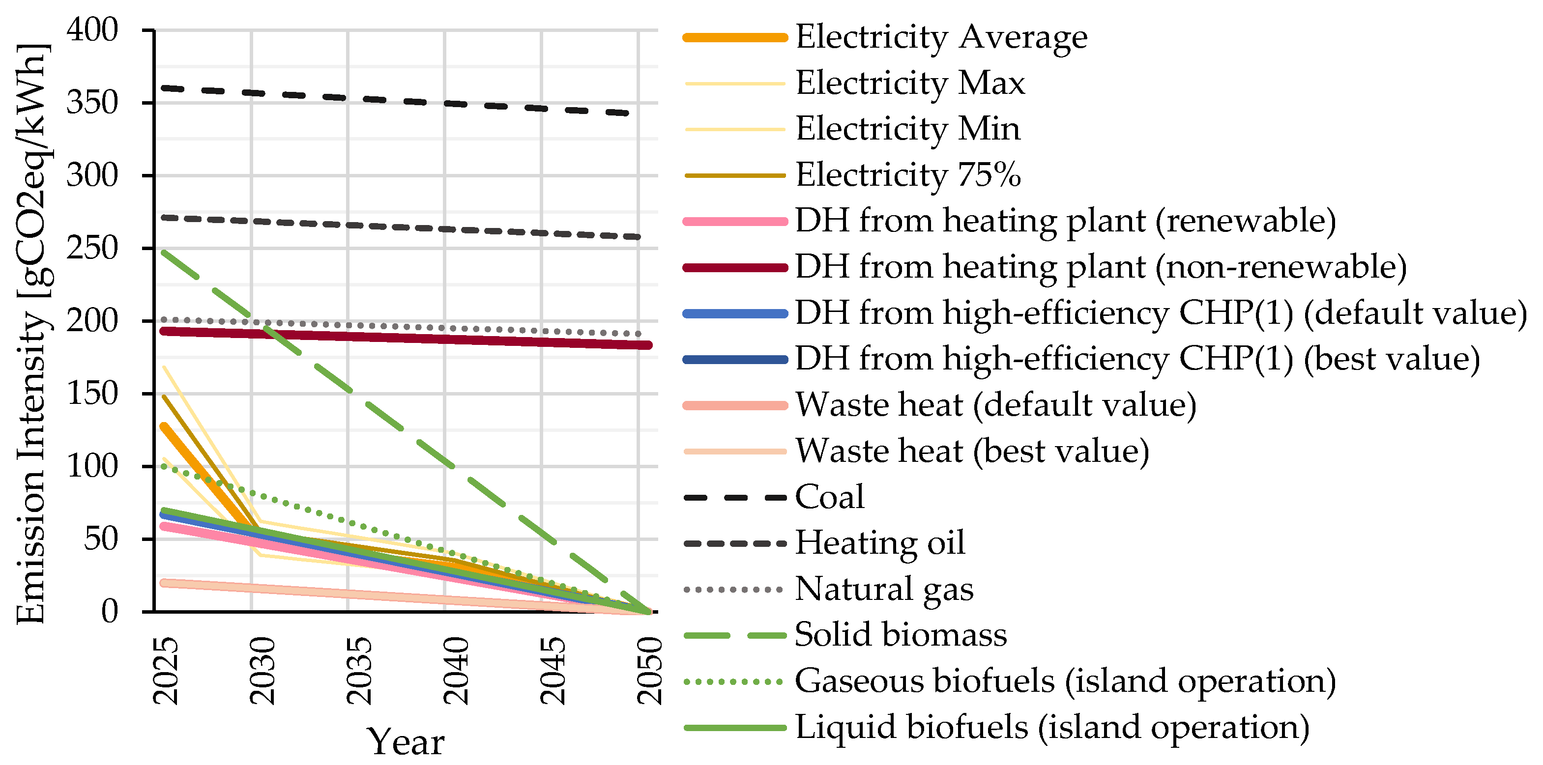
Figure 9.
Primary energy balance of district scenarios (demand and supply side contributions as grid equivalents). Stacked bars illustrate energy demand categories (HVAC, electricity, mobility) and supply contributions (PV own consumption and grid feed-in both visualized as grid substitution equivalent, energy-flexible grid demand equivalent, contextual measures). Scenarios compare fossil and eco construction, enhanced PV deployment, additional mobility measures, and renewable heat supply (GSHP, DH).
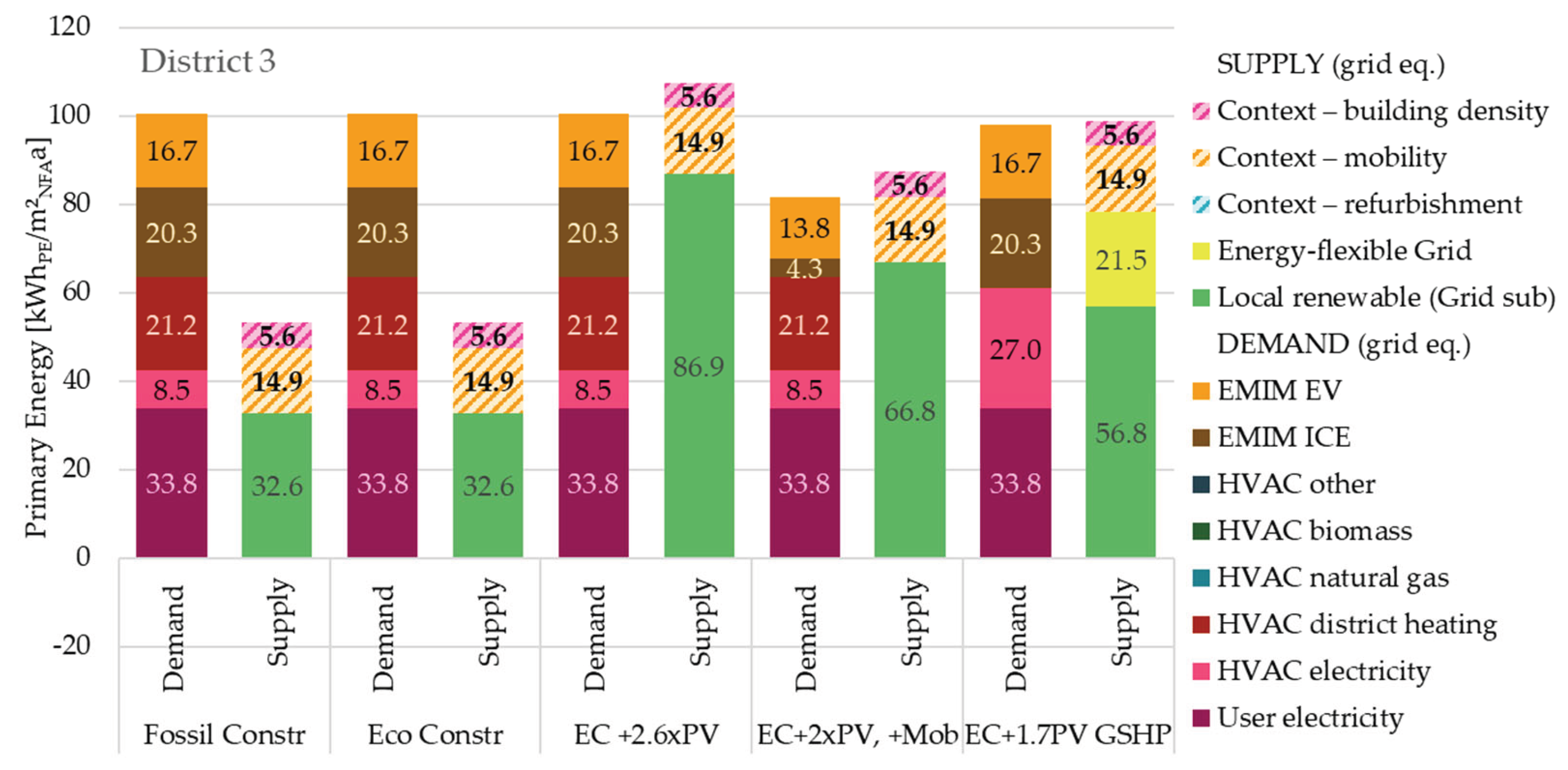
Figure 10.
Grid Emission intensities of different base years (A – Annual, M – Monthly, H … Hourly).
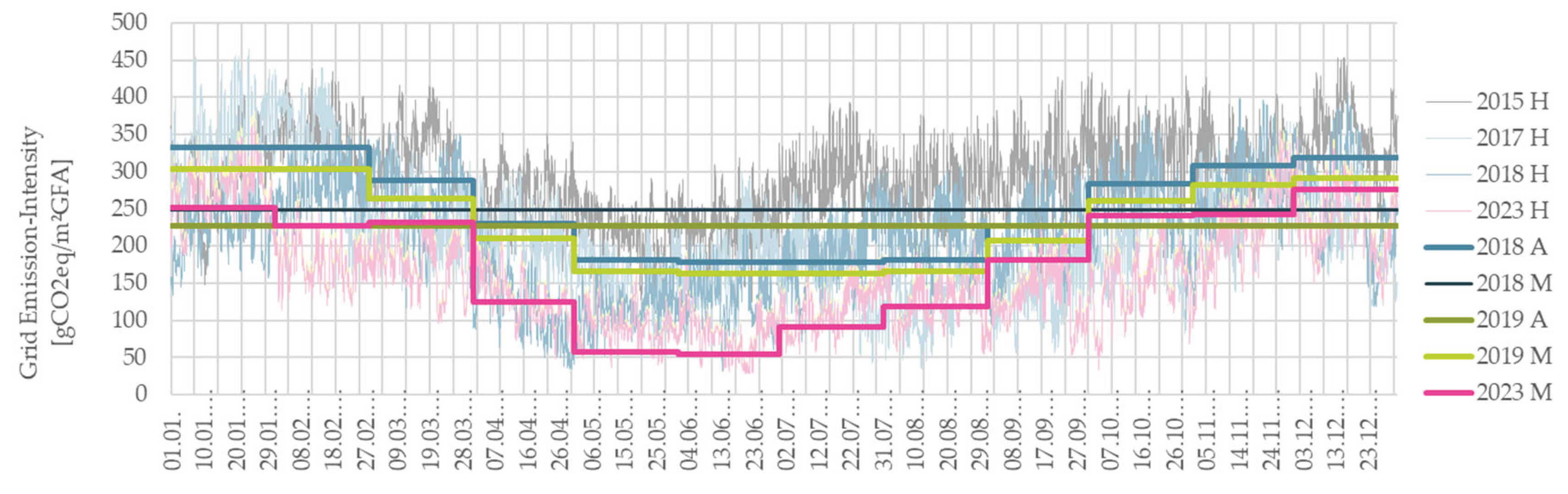
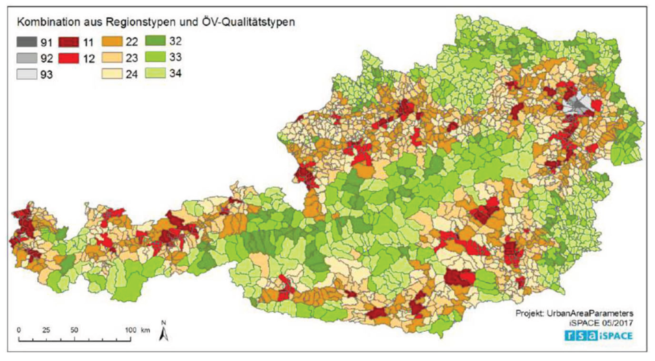
Figure 13.
LCA GHG Emissions from EMIM (B8.1-B8.2) in kgCO₂e·m⁻²GFA, bars showing embodied emissions (EE) and operational emissions over 50 years (OE) for vehicles with internal combustion engines (ICE) and electric vehicles (EV) in kgCO₂e·m⁻²GFA per district Location (region code in Figure 12) and EV Penetration rate (10 – 90%) on the x-axis.
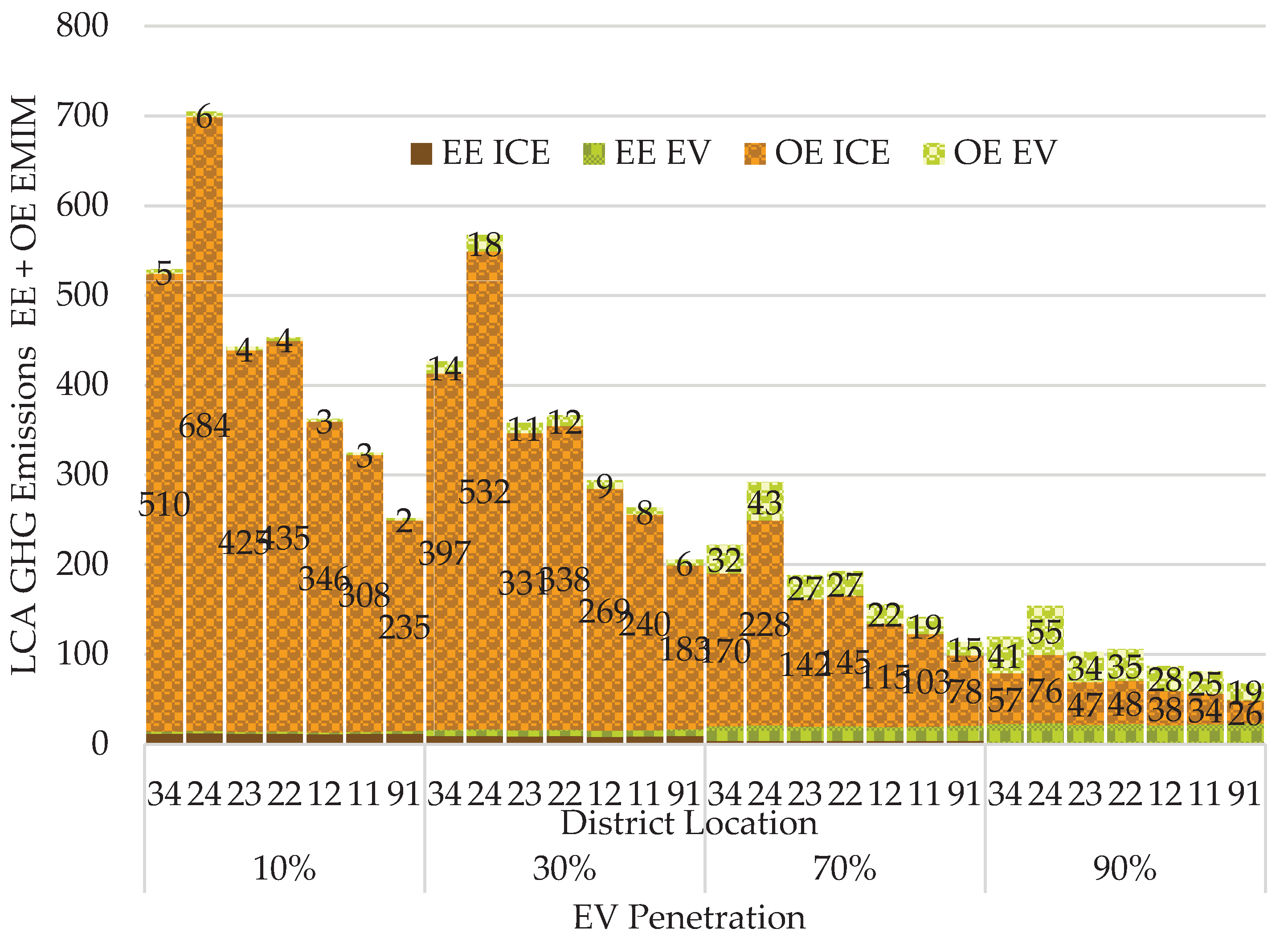
Figure 14.
Cumulative GHG LCA emissions (2025–2075) per m² GFA for seven refurbishment options— status quo (Gas SQ, district heating DH SQ), renovated conventionally (DH Conv-Reno, GSHP Conv-Reno, GSHP Conv-Flex), and ecologically (DH Eco-Reno, GSHP Eco-Reno) under the metropolitan mobility case with 70% EV. Stacks decompose district-operation (B6), EMIM (ICE/EV), TES-related A1–A3, construction A1–A3, avoided grid emissions (D2), and CCS; shaded bands show compliance thresholds (L3 = 320, L2 = 196, L1 = 72 kgCO₂e ·m⁻²).
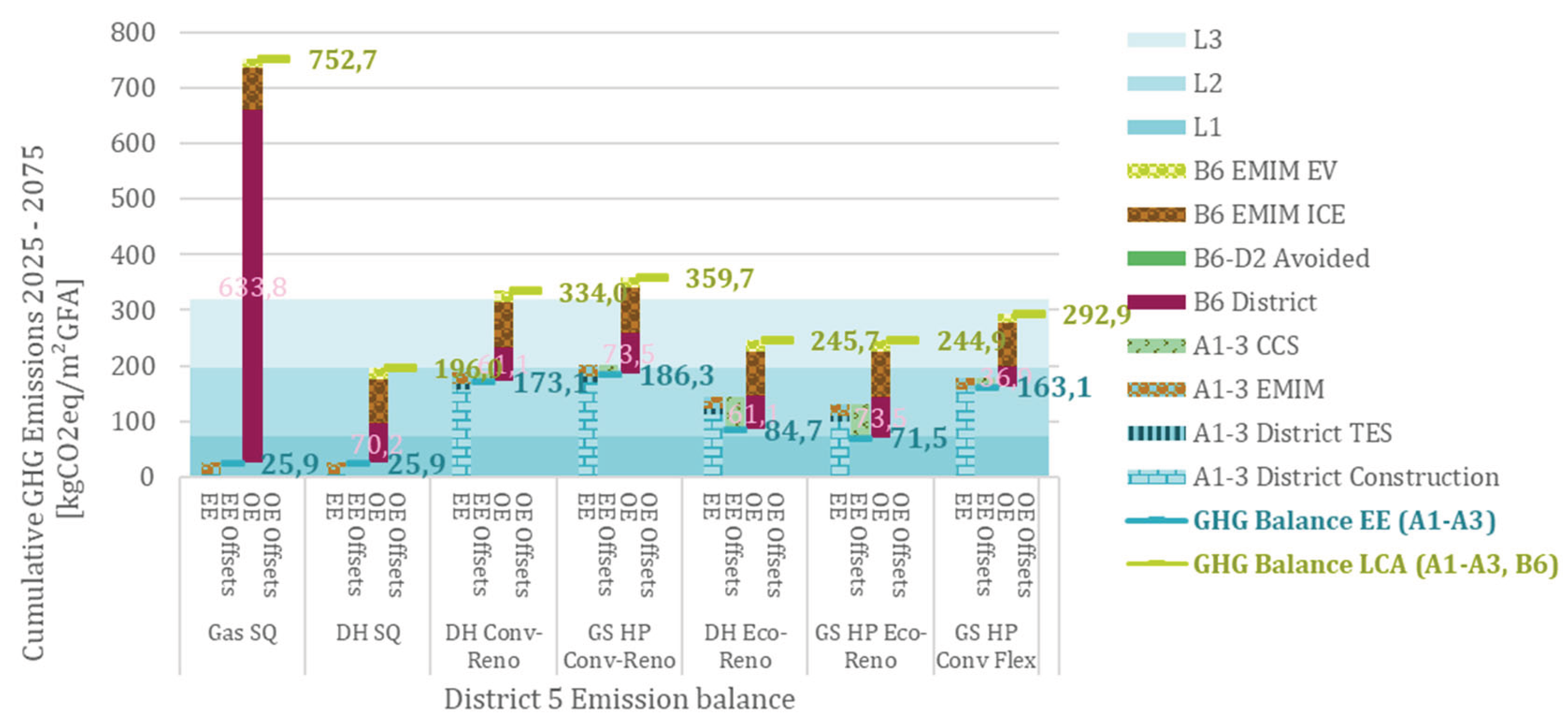
Figure 15.
Annual primary-energy balance (demand vs. supply credits) for D5. Demand stacks show user electricity, HVAC electricity/district heating/natural gas/biomass, other HVAC, and passenger-car fuels; supply stacks show local renewable substitution and energy-flexible supply (TABS load shifting) plus contextual credits.
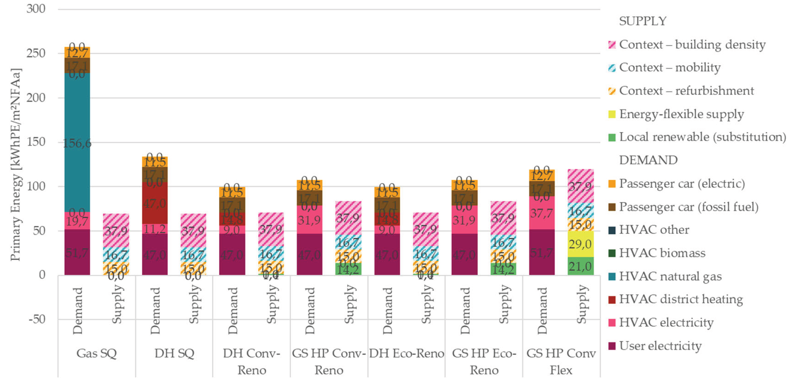
Figure 16.
Embodied (x-axis) vs. Operational incl. EMIM (y-axis) Emissions by location and intervention. Blue lines show cumulative-budget thresholds (solid L3, dashed L2, dotted L1). Fill = EV share (5–100%); outline = thermal system (blue gas, red DH, yellow GSHP); shape = construction choice (■ no renovation, ▲ code, ● ecological).
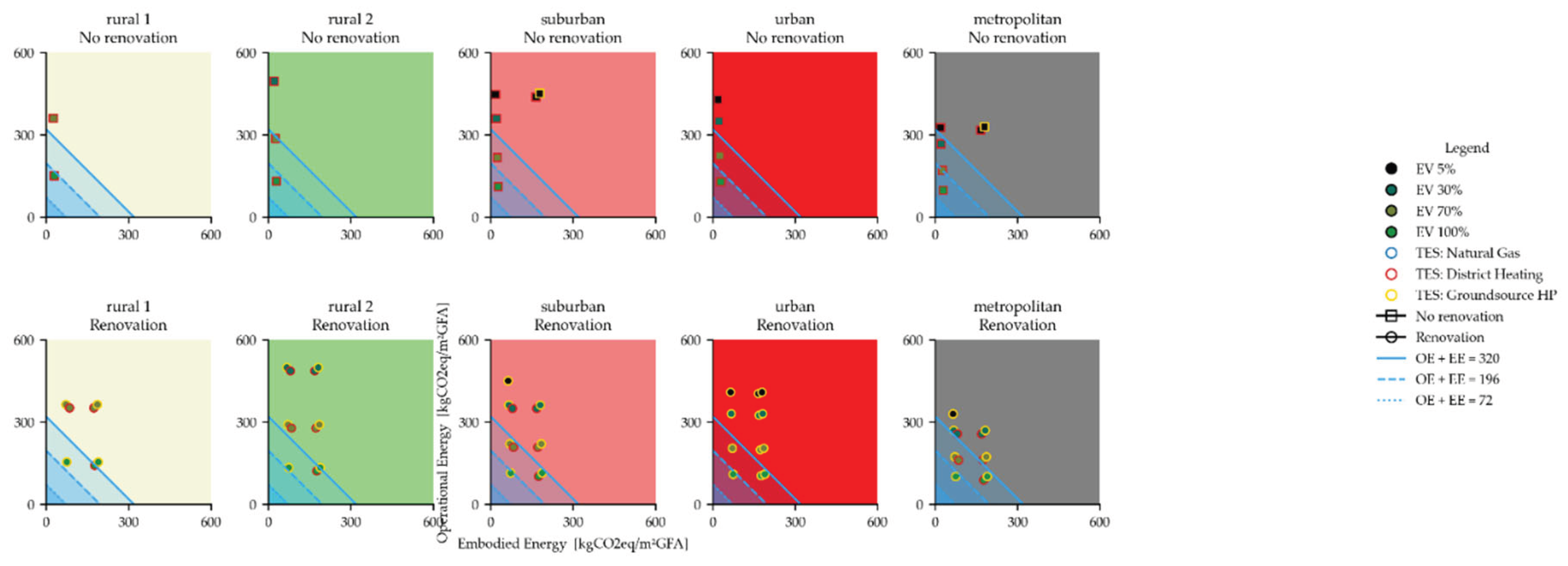
Figure 17.
Cumulative A1–A3 GHG emissions by building component for four D6 concepts (EE stacks only). Bars decompose structure, envelope, interior and TES-related items; negative segments indicate biogenic carbon storage (timber/straw).
Figure 17.
Cumulative A1–A3 GHG emissions by building component for four D6 concepts (EE stacks only). Bars decompose structure, envelope, interior and TES-related items; negative segments indicate biogenic carbon storage (timber/straw).
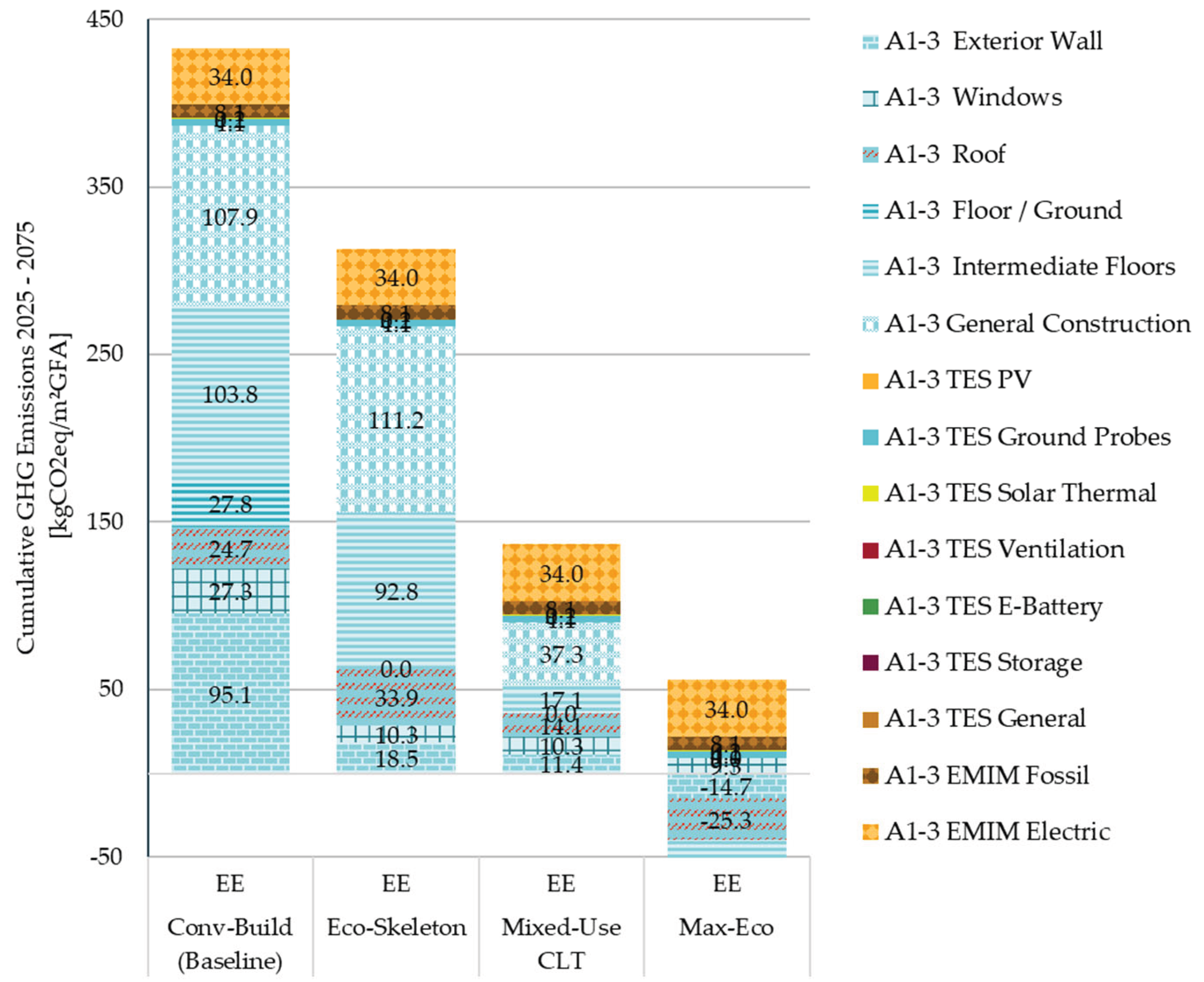
Table 1.
Types of PED as defined in [14].
Table 1.
Types of PED as defined in [14].
| Type of PED | Acronym | Requirements |
| Positive Energy District | PED | PE Balance > 0 excl. EMIM |
| Positive Energy District with Mobility | PED+M | PE Balance > 0 incl. EMIM |
| Climate-Neutral Positive Energy District (reported in this study) |
CN PED | PE Balance > 0 incl. EMIM GHG LCA ≤ L3 over 2025–2075 |
Table 6.
B8 Mobility emission inclusion matrix.
| B8 Emission cause / use | Accounted | Modelled | Emission balance impact | Treatment / rationale |
| Public Transport | ✗ | ✗ | None | Allocated to transport sector; outside district control. |
| Pedestrian, Bike, Other | ✗ | ✗ | None | Negligible at district scale. (Included if not) |
| EMIM ICE Trips to District | ✓ | ✓ | + | Included. |
| EMIM ICE Trips elsewhere | ✗ | ✗ | None | Not included here; attributed to destination system. |
| EMIM EV On-site Charging | (✓) | ✓ | + | Included using hourly source emission factors (grid, local PV = 0) |
| EMIM EV Off-site Charging | (✓) | ✓ | + | Included using hourly grid emission factors. |
| → Trips to District | ✓ | ✓ | (+) | Implicitly included |
| → Trips elsewhere | ✗ | ✓ | – | Deduct grid-equivalent credit to remove out-of-district travel from EV charging OE |
| → V2B discharge | ✓ | ✓ | (+) | Like BESS: Charging included, but lowering building OE at discharge |
Notes: (1) “Emission balance impact”: “+” adds emissions; “−” is a credit.
Table 7.
Total (PEtot), non renewable (PEnre) and renewable (PEre) Primary energy conversion and GHG emission factors for 2024 of selected energy carriers based on [23,48].
| Energy Carrier | PEtot | PEnre | PEre | GHG |
| kWhPE·kWh-1EE | gCO2eq·kWh-1 | |||
| Grid Electricity | 1.76 | 0.79 | 0.97 | 156 |
| District heating – boiler plant (renewable) | 1.72 | 0.4 | 1.32 | 59 |
| District heating – boiler plant (non-renewable) | 1.48 | 1.16 | 0.32 | 193 |
| District heating – high-efficiency CHP (default) | 0.59 | 0.41 | 0.18 | 67 |
| District heating – high-efficiency CHP (best case) | 0.33 | – | 0.33 | 20 |
| Waste heat (default) | 1.00 | – | 1.00 | 20 |
| Waste heat (best case) | 0.30 | – | 0.30 | 20 |
| Coal | 1.46 | 1.46 | 0.00 | 360 |
| Heating oil | 1.20 | 1.20 | 0.00 | 271 |
| Natural gas | 1.10 | 1.10 | 0.00 | 201 |
| Biomass (solid) | 1.13 | 0.10 | 1.03 | 247 |
| Biofuels (gaseous, stand-alone operation) | 1.40 | 0.40 | 1.00 | 100 |
| Biofuels (liquid, stand-alone operation) | 1.50 | 0.50 | 1.00 | 70 |
| District cooling Vienna [49] | 0.42 | 0.13 | 0.29 | 42 |
Table 9.
Assessment model parameter overview. A detailed list of all parameters for the baselineof all example use cases can be found in appendix Tabeappendix A1.
Table 9.
Assessment model parameter overview. A detailed list of all parameters for the baselineof all example use cases can be found in appendix Tabeappendix A1.
| Category | Description of Data | Parameters |
| District | Gross floor areas, net to gross ratios, renovation shares per usage | 24 |
| Weather | Hourly TSD of ambient temperature and N/E/S/W/H Irradiation | 6 x 8760 |
| Heights | Average room heights per usage | 8 |
| Building Hulls | Hull areas by type and orientation | 8 |
| Building Physics | Thermal transmittances, effective heat capacities, heat bridges, air tightness | 10 |
| Windows | Total transmittance, shading offsets summer, winter, mobile shading | 32 |
| Ventilation | Per usage: Share of mechanical/window ventilation, night ventilation, ACH, electricity demand, heat recovery rates | 44 |
| Usage | Concurrencies, DHW demands, auxiliary and plug loads per usage | 35 |
| Lighting | Daylight controls and coefficients, illuminations, light power loads per usage | 12 |
| Heating | Heating periods, Heating Powers and COPs of up to four heating systems (2 electric, 2 thermal), setpoint temperatures | 33 |
| Cooling | Cooling periods, Cooling Powers and COPs of up to 3 active and 1 passive systems (2 electric, 1 thermal, 1 free cooling), setpoint temperatures | 37 |
| DHW | Hot water demand profiles, storage volumes, generation efficiencies, distribution losses | 17 |
| PV Systems | Installed PV capacity, module and inverter efficiency, Hourly TSD of PV yield | 5 + 8760 |
| BESS | Battery capacity, charging/discharging efficiencies, c-rates, losses | 11 |
| Flexibility | Heating, Cooling, DHW, PV, BESS utilization ranges | 11 |
| Mobility | Usage intensity, concurrency, motorization, Annual mileage, EV penetration rates, charging infrastructure, minimum SOCs, utilization of bi-directional charging | 32 |
| Embodied carbon | Construction materials and components, GHG intensities, life cycles, reference areas | 37 |
| PE & Emission factors | Primary Energy and Emission conversion factors, annual weights, context factors | 2 x 8760 13 |
Table 10.
Baseline District Scenarios Comparative compliance summary.
| District | Heat demand kWh·m⁻²NFA·a⁻¹ |
GHG LCA kgCO₂e·m⁻²GFA |
Δ vs L3* kgCO₂e·m⁻²GFA | < L3 | PE Balance kWhPE·m⁻²NFA·a⁻¹ |
> 0 | CN PED |
| D1 | 16.0 | 349.2 | +29.2 | ✗ | 2.8 | ✓ | ✗ |
| D2 | 21.3 | 292.6 | -27.4 | ✓ | 8.2 | ✓ | ✓ |
| D3 | 25.6 | 278.0 | -42.0 | ✓ | -47.7 | ✗ | ✗ |
| D4 | 33.3 | 211.3 | -108.7 | ✓ | 2.8 | ✓ | ✓ |
| D5 | 37.9 | 349.0 | +29.0 | ✗ | -34.3 | ✗ | ✗ |
| D6 | 13.8 | 620.2 | +300.2 | ✗ | 12.8 | ✓ | ✗ |
* Δ vs L3 = GHG LCA − 320; positive = overshoot; negative = undershoot / compliance.
Table 11.
Embodied Emissions of example District PV TES EE in total and relative to the remaining EE and total LCA Emissions.
Table 11.
Embodied Emissions of example District PV TES EE in total and relative to the remaining EE and total LCA Emissions.
| Scenario |
PV Yield kWh·m-2a-1 |
EE A1-A3 w/o PV kgCO₂e·m⁻²GFA |
EE A1-3 TES PV kgCO₂e·m⁻²GFA |
∆EE [%] |
∆LCA [%] |
| D1 | 39.8 | 284.0 | 38.6 | +13.6 | +11.0 |
| D2 | 32.7 | 232.8 | 30.6 | +13.1 | +10.5 |
| D3 | 20.0 | 122.1 | 19.9 | +16.3 | +7.1 |
| D4 | 10.7 | 58.0 | 10.8 | +18.7 | +5.1 |
| D5 | 0.9 | 163.1 | 8.1 | +5.0 | +2.3 |
| D6 | 19.5 | 433.0 | 19.4 | +4.3 | +3.1 |
Table 12.
Summary of case study results for District 3 – urban medium-density residential redevelopment, reporting GHG LCA emissions (kgCO2eq/m²GFA) L3 and L2 compliance, Primary Energy balance and zero PE-Balance and Climate Neutral PED compliance.
Table 12.
Summary of case study results for District 3 – urban medium-density residential redevelopment, reporting GHG LCA emissions (kgCO2eq/m²GFA) L3 and L2 compliance, Primary Energy balance and zero PE-Balance and Climate Neutral PED compliance.
| Scenario | Construction | PV Size | Mobility | TES | GHG LCA* | < L3 | < L2 |
Primary Energy Balance kWhPE·m⁻²NFA·a⁻1 |
Climate Neutral PED | |
| Fossil Constr | Fossil | 1× | 70% EV | DH | 378.2 | ✗ | ✗ | -47.4 | ✗ | ✗ |
| Eco Constr | Ecological | 1× | 70% EV | DH | 277.6 | ✓ | ✗ | -47.4 | ✗ | ✗ |
| EC +2.6xPV | Ecological | 2.6× | 70% EV | DH | 225.6 | ✓ | ✗ | +6.9 | ✓ | ✓ |
| EC+2xPV, +Mob | Ecological | 2× | 90% EV, 80%EMIM | DH | 170.1 | ✓ | ✓ | +5.7 | ✓ | ✓ |
| EC+1.7PV GSHP | Ecological | 1.7× | 70% EV | GS HP | 254.7 | ✓ | ✗ | +0.9 | ✓ | ✓ |
* Unit: kgCO2eq·m⁻²GFA.
Table 15.
Case Study District 5 Factor Variations and resulting Scenarios.
| Factor | Levels (examples) | Unit | How operationalized |
| Location (EMIM mileage) | 34 (Rural-2) / 24 (Rural-1) / 23 / 22 / 12 (Suburban) / 11 (Urban) / 91 (Metropolitan) | km·cap⁻¹·a⁻¹ | Per-capita annual motorized mileage profile |
| EV share | 5 / 30 / 70 / 90 | % of EMIM | Split km into ICE/EV; apply EIc, EFc(t) |
| TES | Gas / DH / GSHP+PV | — | Carrier paths; PV substitution & D2 for feed-in |
| Renovation | None / Conventional / Ecologic | — | A1–A3 inventories; B6 demand |
Table 16.
Sensitivity Analysis of LCA results to TES, renovation and flexibility for District 5.
| Scenario | TES | Renovation | GHG LCA kgCO2e·m⁻²GFA |
L3 Compliance | PE Balance kWhPE·m⁻²GFAa-1 |
PED compliance |
| Gas SQ | Gas | None | 752.7 | ✗ | -188.3 | ✗ |
| DH SQ | DH | None | 196.0 | ✓ | -64.4 | ✗ |
| DH Conv (Baseline) | DH | Conventional | 349.0 | ✗ | -34.3 | ✗ |
| GS HP Conv | GS HP | Conventional | 359.7 | ✗ | -23.7 | ✗ |
| DH Eco-Reno | DH | Ecological | 245.7 | ✓ | -28.5 | ✗ |
| GS HP Eco-Reno | GS HP | Ecological | 244.9 | ✓ | -23.7 | ✗ |
| GS HP Conv Flex | GS HP | Conventional | 292.9 | ✓ | +0.4 | ✓ |
Table 17.
Description of District 6 Scenarios and GHG LCA Results.
| Scenario |
EE A1-A3 |
∆ Baseline |
EE Total |
GHG LCA |
Compliance |
| Conv-Build (Baseline) | 386.5 | - | 433.0 | 620.2 | ✗ |
| Eco-Skeleton | 266.7 | -31% | 313.2 | 500.3 | ✗ |
| Mixed-Use CLT | 90.1 | -77% | 136.6 | 323.8 | d (L3, <320) |
| Max-Eco | -91.0 | -124% | -44.5 | 142.7 | ✓(L2, <196) |
Disclaimer/Publisher’s Note: The statements, opinions and data contained in all publications are solely those of the individual author(s) and contributor(s) and not of MDPI and/or the editor(s). MDPI and/or the editor(s) disclaim responsibility for any injury to people or property resulting from any ideas, methods, instructions or products referred to in the content. |
© 2025 by the authors. Licensee MDPI, Basel, Switzerland. This article is an open access article distributed under the terms and conditions of the Creative Commons Attribution (CC BY) license (http://creativecommons.org/licenses/by/4.0/).
Copyright: This open access article is published under a Creative Commons CC BY 4.0 license, which permit the free download, distribution, and reuse, provided that the author and preprint are cited in any reuse.


