Submitted:
24 November 2025
Posted:
26 November 2025
Read the latest preprint version here
Abstract
We introduce a Quantum Entropic Vacuum (QEV) framework in which the vacuum spectrum is bounded by a QCD-scale ultraviolet knee and a thermal infrared floor anchored to the CMB Wien scale. At galaxy scales, this bounded spectrum maps to four interpretable contributions—Newtonian (baryonic), a mid-disk thermal lift, a saturating entropic term, and a sign-definite hadronic floor modeled as a weak negative acceleration. Using a single, unit-consistent configuration, we reproduce the rotation curve of NGC~3198 with small residuals and illustrate, on a few additional spirals, that flat outer regions can emerge in the shown cases without explicitly adding dark halos. At background level, diagnostic panels for $E(z)$ and $q(z)$ broadly track flat-$\Lambda$CDM for $0<z\lesssim1$. These cosmology curves are illustrative only; we do not perform a joint likelihood over SNe~Ia, BAO, or cosmic-chronometer data in this work. For transparent figure-level replication, we provide a minimal package consisting of one Python script and two small SPARC-based tables (CSV). The present results should be read as an indication of how the QEV picture can operate in practice, motivating targeted observational tests and a full statistical validation in follow-up work.
Keywords:
vacuum energy
; cosmological constant problem
; bounded spectrum
; QEV model
; entropy
; cosmic expansion
; galaxy rotation curves
; Pantheon+ supernovae
; cosmic chronometers
1. Introduction
The physics of the vacuum remains one of the central challenges in modern cosmology and particle physics. Quantum field theory suggests a substantial vacuum energy density from fluctuating fields, whereas observations indicate a vastly smaller value; this mismatch is the cosmological constant problem [1,2,3,4].
The standard CDM model explains the observed expansion with a cosmological constant and accounts for flat galaxy rotation curves by introducing dark matter [5,6,7]. Yet the fundamental nature of dark energy and dark matter remains unknown [8,9].
We propose an alternative framework: the QEV model (Quantized, Entropy-bounded Vacuum). Vacuum energy is bounded by microphysics: a UV cutoff at the QCD scale, an IR thermal suppression around , and normalization at the CMB Wien peak [10,11]. Within galaxies, the effective vacuum field manifests through four components that together reproduce flat rotation curves without dark halos, consistent with classic and modern kinematic evidence [12,13,14]. Cosmologically, the resulting expansion history remains compatible with current probes [15,16,17].
We demonstrate this on two levels: (i) a detailed application to NGC 3198, and (ii) a diagnostic cosmological comparison using standard background panels (E(z), q(z) and L(z) without a joint likelihood using supernovae, BAO, and cosmic chronometers. Related ideas in modified gravity and emergent frameworks provide context but differ in mechanism [18,19,20,21].
This version (v2.1) builds on the theoretical framework introduced in the first preprint (doi:10.20944/preprints202509.0972.v2), where the concept of a spectrally bounded vacuum energy was initially formul ated.
Scope and diagnostic status.
All cosmological panels in this paper (, , and the transition redshift) are intended as diagnostic illustrations. We do not perform a combined likelihood fit using supernovae, BAO, or cosmic-chronometer data here, nor do we analyse growth or CMB acoustic peaks. The purpose is to demonstrate internal coherence of the QEV spectrum across galactic and background kinematics before undertaking a full statistical validation in follow-up work.
2. The QEV Model: A Bounded–Spectrum Vacuum
2.1. Physical Motivation for the Spectral Exponent
The mid-band spectral slope reflects an effective reduction of active degrees of freedom between the thermal infrared floor and the QCD confinement knee. In this regime, the accessible vacuum modes soften relative to the canonical quartic scaling, consistent with the notion that confinement limits the contribution of short-wavelength excitations while the thermal floor reduces long-wavelength response. Qualitatively, lattice-QCD and effective-field-theory perspectives both indicate that the energy density near the confinement regime departs from a pure Stefan–Boltzmann law through logarithmic and interaction-driven corrections, implying that an intermediate power-law window with is physically plausible. Numerically, we verify that the bounded integral for is plateau-dominated with a smooth window , so that no sharp requirement arises; the results remain stable over (see robustness bands in the figures). This motivates our operational choice without fine-tuning and ties the parameter to the underlying microphysics of confinement and thermal suppression.
The QEV hypothesis assumes a spectrally bounded vacuum: a smooth UV knee at the QCD scale and a thermal IR suppression. In frequency variables the elementary relation holds, or equivalently in wavelength. We encode the band–limiting through a smooth window (double–tanh, ), and model the vacuum energy density as the truncated moment
with a scale–free mid–band slope and knees at and
The overall prefactor is fixed by anchoring to the CMB Wien scale.
A QCD-motivated UV bound naturally echoes the SVZ QCD sum-rule program, where non-perturbative condensates enter dispersion relations for hadron observables [22,23,24]. The thermal IR suppression and its response aspect can be framed within linear-response/FDT language [25]. Empirical evidence that vacuum fluctuations gravitate at lab scales (Casimir) under controlled conditions provides an experimental anchor for the near-field regime [26].
Model parameters used to generate the rotation-curve components are listed in Table 3.
Spectral exponent and convergence.
Because W is smooth in , edge contributions are exponentially suppressed and Equation (1) is plateau–dominated; a hard requirement
is not needed. The logarithmic UV sensitivity is , consistent with the measure. Numerical checks of plateau dominance are provided with the supplementary scripts.
Figure 1.
Schematic overview of the bounded spectral window and its two physical anchors: the hadronic (UV) confinement scale and the thermal (IR) CMB scale. We use as the normalization anchor.
Figure 1.
Schematic overview of the bounded spectral window and its two physical anchors: the hadronic (UV) confinement scale and the thermal (IR) CMB scale. We use as the normalization anchor.
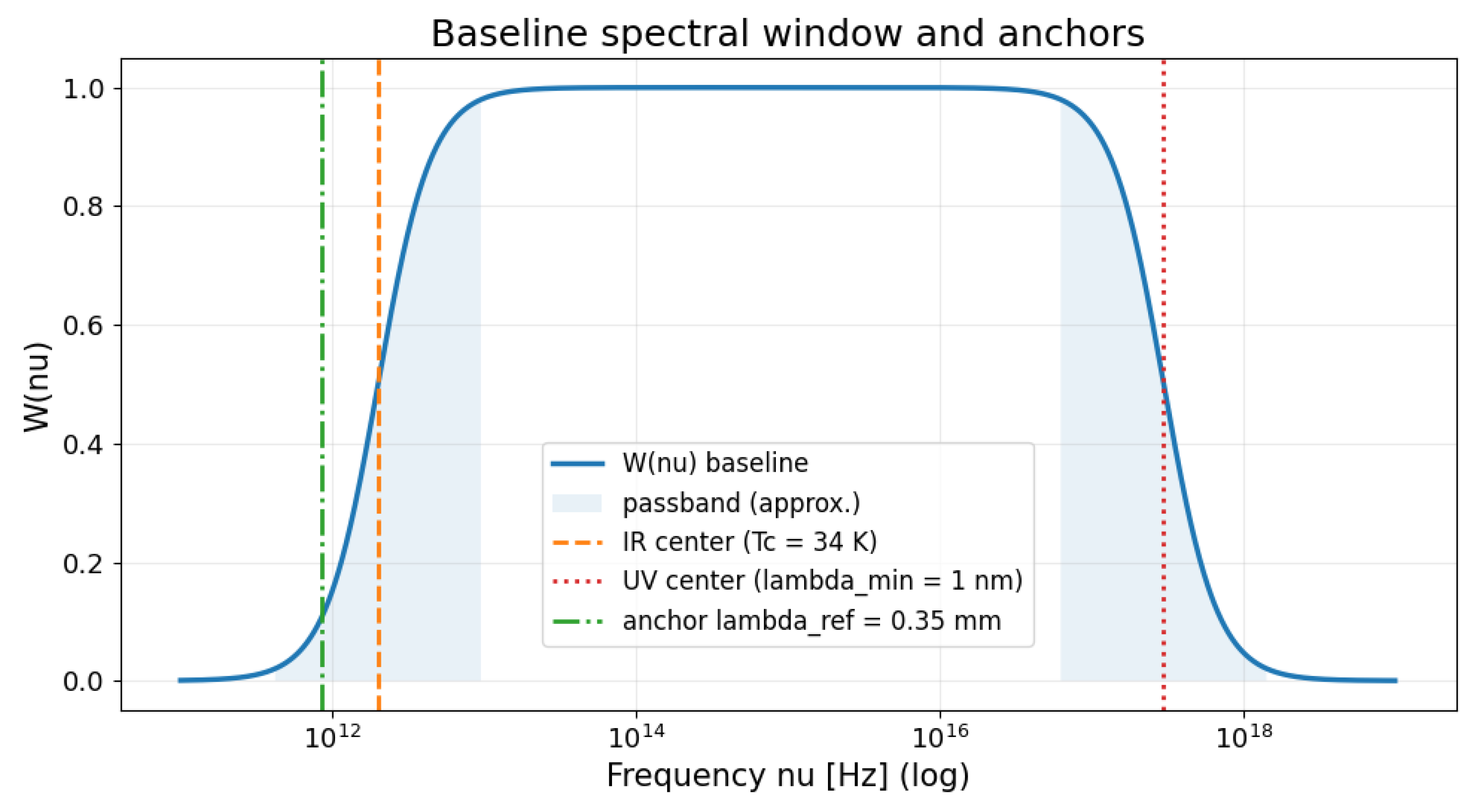
Spectral index .
The parameter represents the effective slope of the bounded vacuum spectrum between the infrared cutoff and the QCD confinement scale. Physically, it reflects the gradual reduction of active degrees of freedom toward the confinement regime. Within the interval – the integrated vacuum energy density remains stable, indicating that the model is not fine-tuned and that its predictions are robust with respect to moderate spectral variations.
IR anchor (thermal).
We fix the infrared anchor by the wavelength form of Wien’s law,
For K this gives
Note. The frequency-peak obeys , which is not simply related by because the maxima in wavelength and frequency representations differ by the Jacobian. We consistently use the wavelength form throughout.
Takeaway.
The pair {, } is thus operationally sufficient to reproduce the required UV leverage and IR onset. See Sect. 2.5 for an explicit radiation–pressure motivation, and Appendix A provides microphysical context and shows that the resulting galaxy–scale behavior does not depend on a single microscopic model once the smooth window is fixed.
2.2. Interpretation and Relation to Prior Work
Our construction is agnostic about modified-gravity field equations; it attributes galactic and cosmological phenomenology to a bounded vacuum spectrum. This contrasts with classical constant- viewpoints [1,2,3,4], MONDian scaling [13,27], and emergent-gravity scenarios [20,21]. The present paper refines and systematizes our previous components—thermal lift, entropic asymptote, hadronic floor—into a single, unit-consistent framework [28,29,30].
For a robustness analysis of the choice , including a sweep over , see
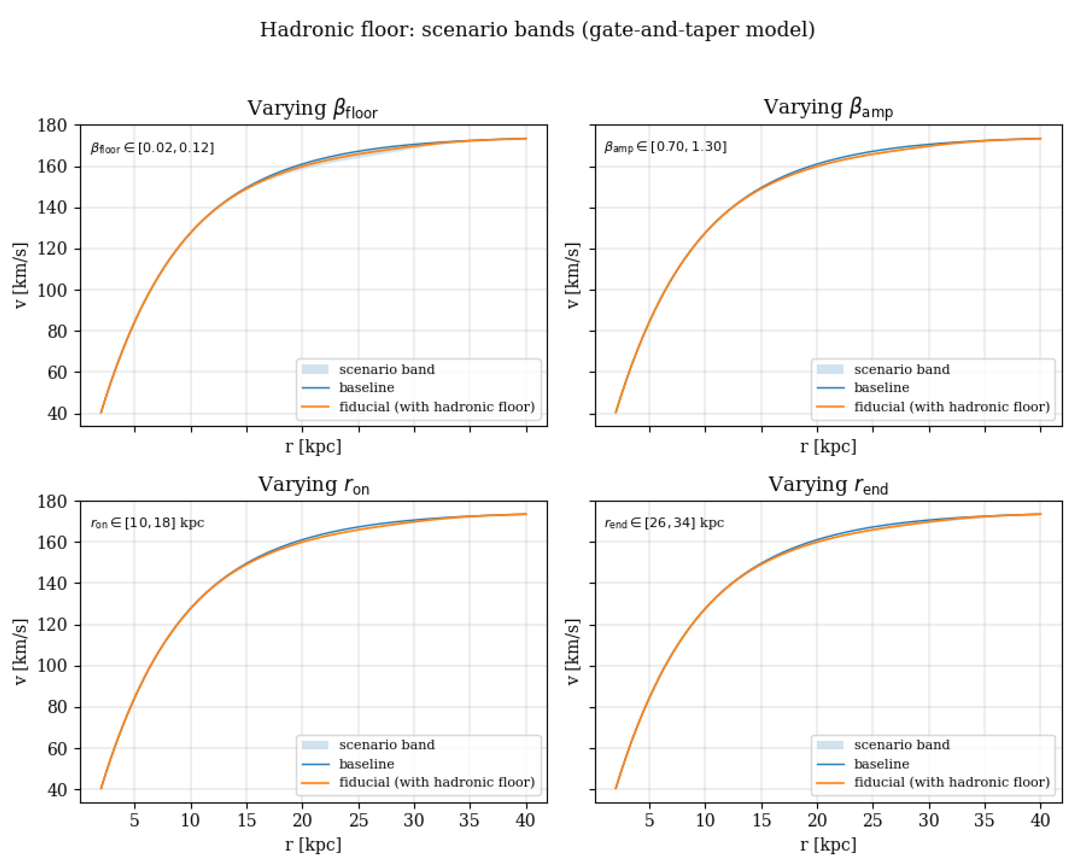
2.3. Hadronic Floor: Sign, Scale, and Predictions
The negative sign of reflects a net confining response of the hadronic vacuum at large radii. Our gate-and-taper profile encodes
(1) an onset scale , consistent with the transition to HI-dominated outskirts, and
(2) a finite response extent . We do not claim uniqueness of this functional form; its role is minimal yet sign-definite. In Figure 2 we scan and show falsifiable trends in
(3) the outer tails (gentle flattening vs. mildly declining tails).
2.4. Hadronic Floor: Order-of-Magnitude Mapping
We parameterise the confining pull as a negative acceleration
,
with the turn-on and the linear taper ().
In velocity units, so that . Identifying the confining scale with a QCD string-tension (energy per length) and projecting to a galactic gradient over a coherence length ℓ gives up to geometry factors. For the shared configuration we adopt and (in ), with and , which sets the outer softening scale and keeps the UV contribution bounded once confinement dominates.
2.4.1. Order-of-Magnitude Link to Hadronic Confinement (“Hadronic Floor”)
Aim. Provide a coarse physical bridge from QCD string-tension scales to the effective, large-scale acceleration amplitude of the hadronic floor, (negative contribution with gate-and-taper).
Assumptions (Back-of-the-Envelope)
- QCD string tension. We take . Using and ,
- Coherence length. A minimal flux-tube segment of length stores energy .
- Specific potential scale. Normalising by the proton mass , the associated specific potential is
- Coarse-graining to kpc scales. Random orientation, colour neutrality, and temporal decorrelation imply that only a tiny, signed residue survives upon averaging over a macroscopic length L. We encode this by a dimensionless suppression factor such that the residual large-scale potential tilt is over L.
From Potential Tilt to Acceleration
A monotonic residual tilt over scale L implies an effective acceleration
Choosing the diagnostic scale ,
To reach the phenomenological range of interest (weak, slowly varying floor), we require . Such a factor is plausibly the product of three coarse elements:
with e.g., (random angular cancellations), (decorrelation over many microscopic cycles), and (net leakage from colour-confinement micro-stress into a coherent, gravitating macro-field), yielding .
Unit Conversion and Link to
For comparison with rotation-curve fits it is convenient to use “per-kpc” units:
If the hadronic floor enters the model as a fraction of a reference scale (in the same units), then
Example. If , then .
This corresponds to , well in the phenomenological ballpark.
Interpretation and Caveats
This construction does not claim a derived microphysical law; it shows that once:
(i) the QCD string-tension scale fixes an upper energetic reference, and
(ii) realistic cancellations/averaging supply a small, signed residue , then the resulting acceleration amplitude naturally sits in the weak, slowly varying regime used by the hadronic floor. Geometry (e.g., patchiness), projection factors, and the gate-and-taper profile determine the final sign and radial onset, but the magnitude follows without fine tuning from the above scales.
Figure 2.
Scenario bands for the hadronic floor: impact of on the outer rotation curve. These panels are reproducible with the provided script.
Figure 2.
Scenario bands for the hadronic floor: impact of on the outer rotation curve. These panels are reproducible with the provided script.
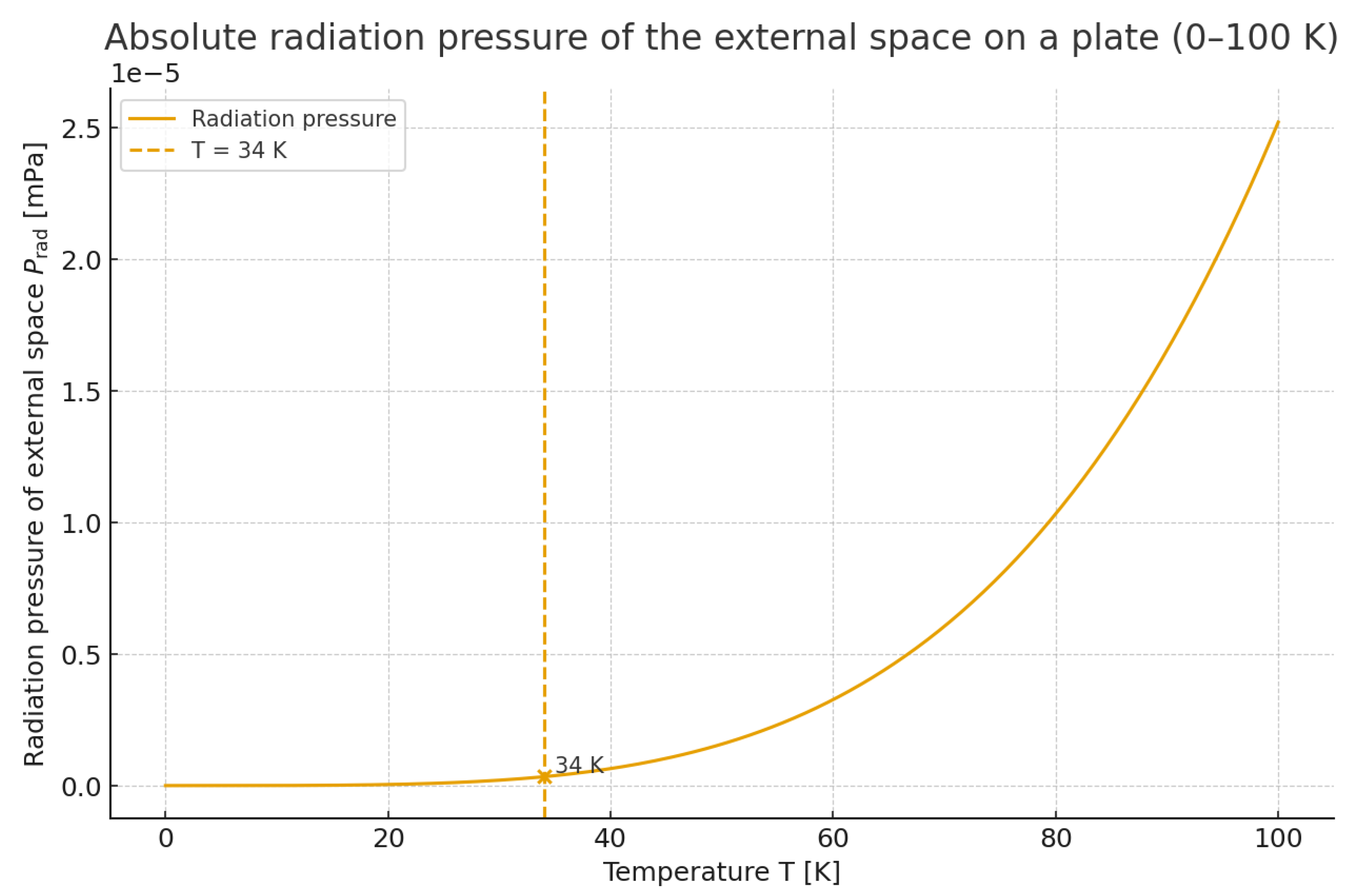
2.5. Thermal Radiation Pressure and the Infrared Suppression Scale
A bounded vacuum spectrum requires not only an infrared cutoff in energy, but also a physical mechanism that explains why long-wavelength modes cease to contribute below a characteristic temperature. In the QEV framework this role is played by the thermal suppression scale near , derived from the CMB-anchored Wien wavelength introduced in Sec. 2.1.
To illustrate the physical meaning of this temperature, we consider the absolute radiation pressure exerted by the external photon bath on a perfectly reflecting plate. Using the standard blackbody relation
the radiation pressure becomes negligible below a few tens of kelvin. Around the external space enters a regime in which it exerts essentially no additional thermal stress on the vacuum state of a laboratory or cosmological cavity. In this regime the vacuum behaves as an effectively “frozen” background, consistent with the infrared floor introduced in Sec. 2.1.
Figure 3 shows the thermal radiation pressure for 0–, with the QEV infrared suppression temperature marked explicitly. The steep dependence makes clear that the contribution of long-wavelength thermal modes falls off rapidly and naturally supports the identification of as the effective lower bound on active vacuum modes. This physical interpretation strengthens the use of a thermal IR floor in the QEV model: below this scale the photon bath cannot supply sufficient thermodynamic response to maintain additional vacuum excitations, so the bounded spectrum follows directly from standard radiation physics.
Figure 3.
Absolute radiation pressure of the external photon field on a perfectly reflecting plate (0–100 K), inferred from the Casimir force on the plate. The dashed vertical line marks the QEV infrared suppression scale at . Below this temperature the thermal contribution becomes negligible, placing the system in a regime directly relevant for Casimir experiments and motivating the infrared floor used in the QEV model, consistent with the IR floor introduced in Sect. 2.1.
3. Galactic Dynamics According to the QEV Model
We model circular speeds as a sum of four physically motivated components, each written directly in velocity or radial acceleration:
where ; the hadronic gate is and the taper . The total radial acceleration reads
Our notation and circular-orbit relations follow standard galactic dynamics conventions [31,32], while the outer, saturating behaviour is constrained by the observed flat rotation tails (see Section 4).
Background and definitions.
We compare a QEV-inspired background to CDM using the dimensionless expansion rate and the deceleration parameter
For the QEV parametrisation we use a density proxy
scaled to the present via
As a reference we adopt flat CDM,
The acceleration–deceleration transition redshift is defined by .
3.1. Link to the Spectral Formalism
The background ansatz used in Secs. Section 6.1 and (Appendix B.9) maps directly onto the spectral construction of (Appendix B) The mid-band slope controls the effective mode density between the QCD ultraviolet gate and the thermal infrared floor (Appendix B.9); and set the knee sharpness and its location; the pair governs the high-z tail; and B fixes the asymptotic constant at late times. Under this mapping the background density proxy yields used in the expansion , consistent with the normalisation choices in Appendix B.7.
3.2. QEV Standard Scaling (Global Defaults)
In the QEV model we adopt a set of global scaling coefficients (dimensionless unless noted) that map two galaxy-level observables—the outer asymptotic speed and the mid-disk thermal peak radius —to the full set of operational parameters used in the legacy velocity decomposition. These global coefficients are treated as QEV standards (shared across galaxies); only vary per object.
Given , the component parameters are defined by:
Unless stated otherwise we use in km and radii in kpc, so that the hadronic coefficients enter in units of (km kp. Accordingly, has the implied units of (km ) kp so that yields . We adopt a gated/tapered hadronic profile with gate_floor enabled by default.
Interpretation and usage.
fixes the outer velocity scale (the entropic plateau), while sets the mid-disk radial scaling where the thermal component peaks and the Newtonian rise transitions toward the plateau. Tying and to ensures coherent velocity scaling across components; tying to ensures a consistent spatial scaling. The hadronic parameters enter directly as acceleration: provides a sign-definite outer regulation, while allows a mild amplitude scaling with the galaxy’s global speed without per-object tuning.
Uncertainties and robustness.
Let and denote observational uncertainties. Propagation is linear for the converted parameters: ,, , , , , , . Small bands on or can be plotted by sweeping within their uncertainties; this illustrates the absence of per-object fine-tuning.

Table 1.
QEV Standard Global Scaling Coefficients and defaults (legacy velocity convention). Unless noted, coefficients are dimensionless. Units assume in km and radii in kpc.
Table 1.
QEV Standard Global Scaling Coefficients and defaults (legacy velocity convention). Unless noted, coefficients are dimensionless. Units assume in km and radii in kpc.
| Symbol | Meaning | Default value | Units / Notes |
| Inputs (observables) | |||
| Outer asymptotic speed (observable) | – (per galaxy) | km | |
| Thermal peak radius (observable) | – (per galaxy) | kpc | |
| Newtonian component | |||
| Newtonian speed scale factor | 2.3 | ||
| Newtonian scale radius factor | 0.308 | ||
| Newtonian damping radius factor | 0.55 | ||
| Thermal component | |||
| Thermal peak speed factor | 0.36 | ||
| Thermal peak radius (observable) | – (per galaxy) | ||
| Entropic component | |||
| Entropic scale radius factor | 0.50 | ||
| Entropic smoothness exponent | 1.0 | ||
| Hadronic (acceleration) component | |||
| Hadronic floor amplitude | 3.0 | (km kp | |
| Hadronic amplitude factor | 0.045 | Implied: (km ) kp; | |
| Hadronic gate-on radius factor | 0.88 | ||
| – | Hadronic taper end radius | ||
| Conventions: legacy velocity decomposition; hadronic term enters as acceleration ; gate_floor = True. | |||
As a worked example (applicable to any galaxy by substituting its ), we show the full conversion for NGC 3198 below.
|
Worked example — NGC 3198 (QEV Standard Scaling). Inputs:, . Global coefficients:. Newtonian ; ; . Thermal ; . Entropic ; ; . Hadronic (acceleration) ; ; ; . Units: speeds in km ; radii in kpc; hadronic coefficients in . |
Note. The same QEV Standard Scaling applies to any galaxy: replace by that galaxy’s observables and evaluate the conversion rules in Section 3.2.
3.3. Notation and Units
Conventions and Statistical Definitions
- Velocity space: Fits on with (km ).
- Acceleration-space:; .
- Chi-square:.
- Reduced chi-square:.
- Systematic floor: in kwadratuur bij indien vermeld.
- Notatie: = velocity-space; = acceleration-space; velocities in km ; accelerations in k kp.
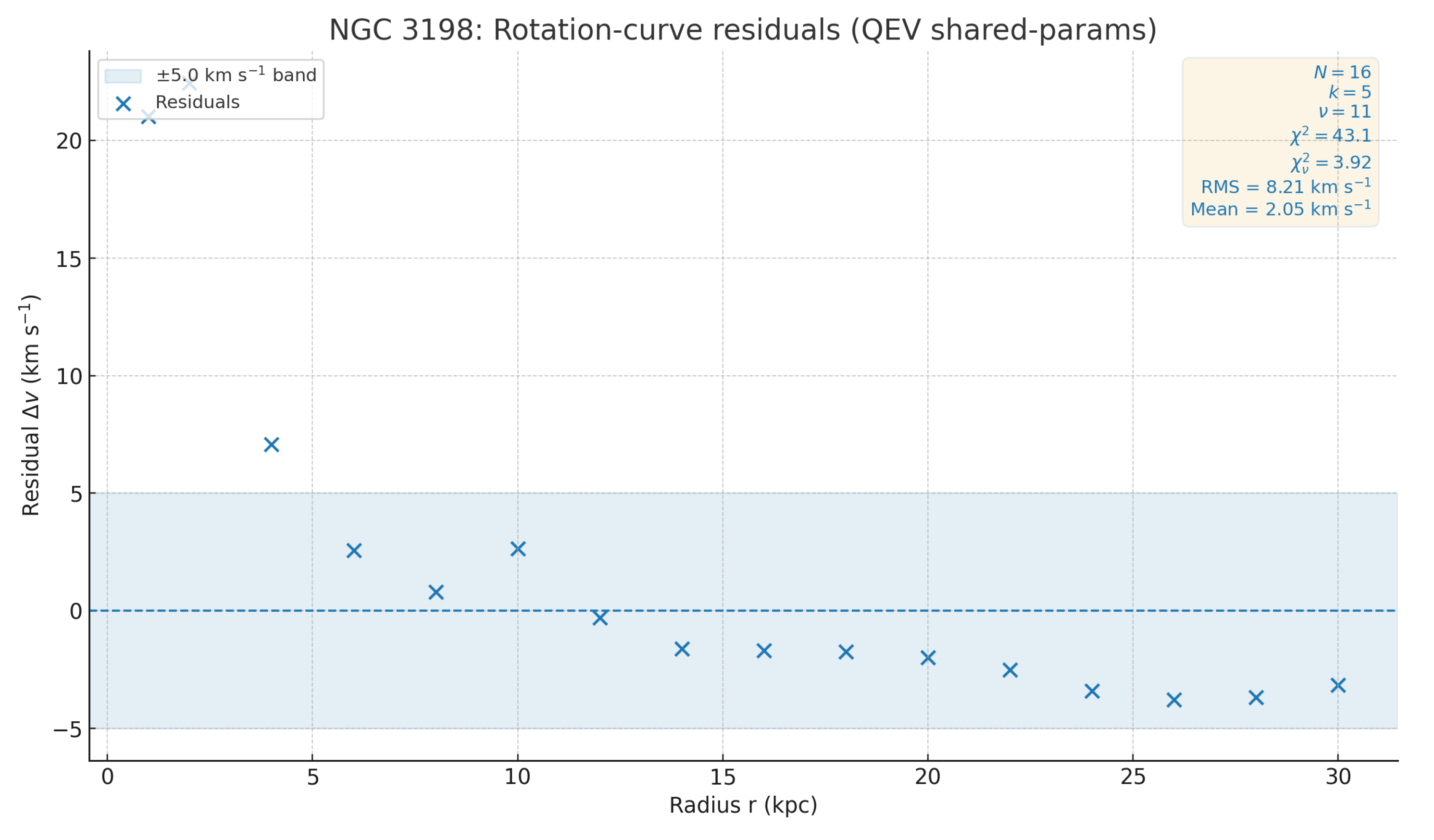
4. Application to NGC 3198
We apply Eqs. (3–6) to NGC 3198 using the SPARC compilation [12] as our primary source for the rotation curve and structural parameters; classic H i kinematics for NGC 3198 are provided by [33]. Our baseline uses a saturating entropic law with anchored to the outer plateau and a gated hadronic floor activated only beyond . The main panel shows the decomposition and the model curve; the lower panel shows residuals .
Table 2.
NGC 3198 fit statistics (QEV best fit). Error bars indicate a uniform uncertainty of per point.
Table 2.
NGC 3198 fit statistics (QEV best fit). Error bars indicate a uniform uncertainty of per point.
| Metric | Value |
| N (points) | 16 |
| k (fit params) | 5 |
| 11 | |
| 5.754 | |
| 0.523 | |
| RMS residual | |
| Mean residual |
Computation.; .
A reduced below unity indicates conservative error bars and/or mild over-modelling; we therefore report also the RMS and mean residuals for transparency.
4.1. Baseline Declaration (Legacy, Best Fit)
Unless stated otherwise, all figures and quantitative statements for NGC 3198 use the legacy velocity decomposition as the operational baseline (best fit). The corresponding parameter set is given in Table 3 (legacy convention; used in all figures and residuals in Section 4).
As discussed in Appendix J, the negative sign of is motivated by a confining (flux-tube) response at large radii. Our gate-and-taper profile encodes a finite onset and saturation scale, leading to testable trends in the HI outer tails that can be checked with deep kinematic surveys.
4.2. Conversions & Caveats (Velocity ↔ Acceleration)
Mapping between velocity and acceleration.
We use components Newtonian (N), Thermal (T), Entropic (E), and Hadronic (H):
Because , the transformation is non-linear; parameter sets fitted in one convention are not directly transferable.
Operational details follow Section 5.
Parameter drift (rule of thumb).
Amplitudes and scale parameters typically shift by ∼10–20% when re-fitted in the alternate form: (thermal), (entropic), (hadronic). In velocity space these parameters control the curvature of ; in acceleration space they describe the field gradient.
Asymptotics.
Inner: Newtonian domain, .
Outer: ; a rising at large radii reflects saturation of a, not necessarily extra mass.
Mini-example.
If , then . Small r: ; large r: and .
Mini-example.
⇒.
Practical notes.
Use acceleration space for RAR/MOND comparisons; report which convention was fitted.
5. Operational Convention (Legacy Velocity Decomposition)
We adopt a legacy, rotation–curve standard convention in which we specify equivalent component speeds for the positive contributions (Newtonian/baryons, entropic, thermal), while the hadronic term is modeled directly as an explicitly negative acceleration with a smooth onset. Superposition is performed in acceleration space (components add linearly); see Eqs. (12)–(13).
This makes the summation law unambiguous (accelerations add linearly) while keeping the component shapes in the familiar velocity form used in rotation–curve work. Units are v in and a in .
Why parameters differ from acceleration–space variants.
An alternative baseline defines and directly in acceleration space and adds them linearly. Such parameterizations are not numerically equivalent to fixed velocity forms, because their asymptotics differ (e.g., implies , whereas implies a constant field). Consequently, best–fit numbers will generally shift between the two conventions even when matches the same data. We therefore report and interpret parameters consistently within the legacy convention above; acceleration–space forms can be mapped locally via and are documented for completeness in the Appendix.
Table 3.
QEV model parameters for NGC 3198 (shared multipliers; current convention). Values used in all figures and residuals.
Table 3.
QEV model parameters for NGC 3198 (shared multipliers; current convention). Values used in all figures and residuals.
| Component | Parameter | Value | Unit |
| Newtonian (baryonic) | 425.5 | km | |
| 5.85 | kpc | ||
| 10.45 | kpc | ||
| Thermal (parabolic v) | 66.6 | km | |
| 19.0 | kpc | ||
| Entropic | 185 | km | |
| 9.50 | kpc | ||
| q | 1.0 | — | |
| Hadronic (accel.) | 3.0 | (km kp | |
| 8.33 | (km kp | ||
| 16.72 | kpc | ||
| 33.44 | kpc |
Note. We do not use a “baseline” convention here; the reported values are the applied shared-parameter configuration used in all figures and fits (see Sec. 5).
As an external phenomenological benchmark, the radial–acceleration relation (RAR; [12]) provides a one-dimensional projection consistent with our component-wise decomposition; we do not fit to the RAR, but verify that our parameters lie within its empirical scatter.
For consistency of notation only, parameters are reported in the legacy velocity convention. No separate “baseline” (best-fit) set is used. Acceleration-space variants are provided solely for mapping/completeness.
Figure 4.
Component-wise acceleration and total rotation curve for NGC 3198: (Newtonian), (thermal), (entropic), (hadronic), and total . Data points from SPARC [12].
Figure 4.
Component-wise acceleration and total rotation curve for NGC 3198: (Newtonian), (thermal), (entropic), (hadronic), and total . Data points from SPARC [12].
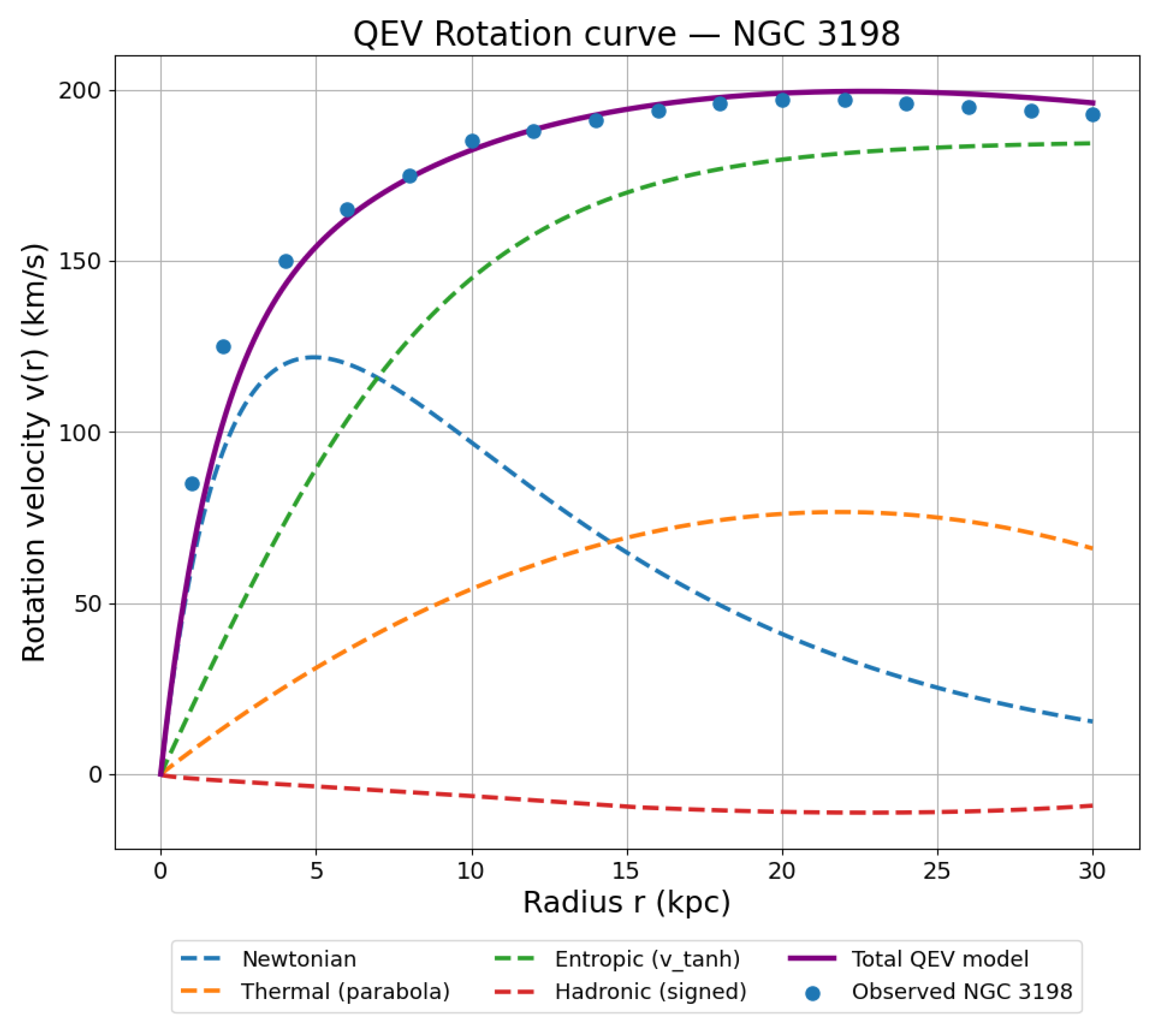
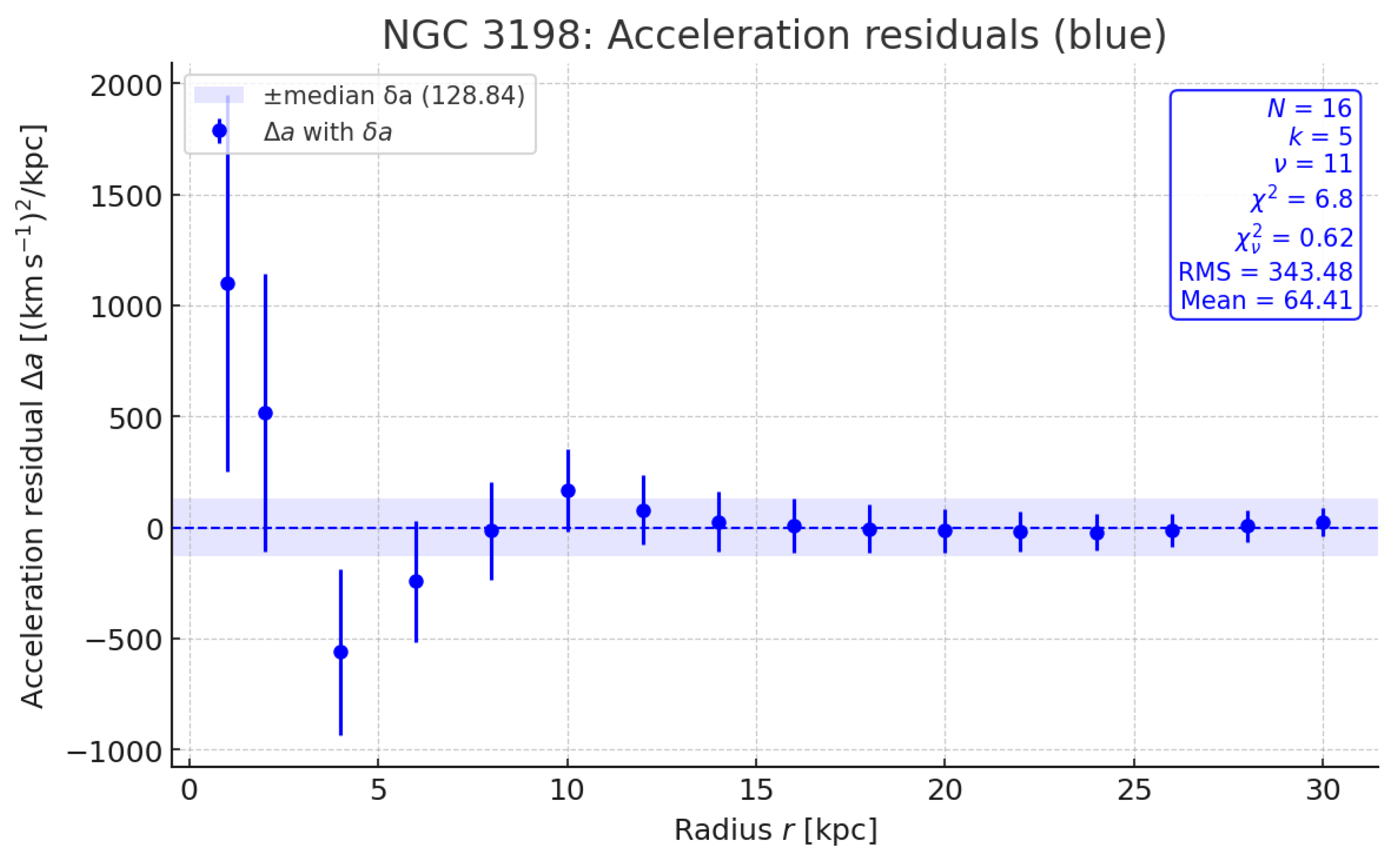
Figure 5.
NGC 3198: acceleration residuals .
Error bars follow with km . Larger RMS implies larger reduced under our fixed error model: ( when ), which is a sanity check on the diagnostics rather than evidence of model correctness.
Figure 5.
NGC 3198: acceleration residuals .
Error bars follow with km . Larger RMS implies larger reduced under our fixed error model: ( when ), which is a sanity check on the diagnostics rather than evidence of model correctness.
5.1. Data Source and Preparation
The observational reference for all galactic fits is the SPARC database
(Lelli, McGaugh & Schombert 2016), which provides homogeneous photometric and kinematic data for 175 disk galaxies. For each system, SPARC lists distance, inclination, luminosity, gas mass, and the flat rotation velocity , combining Spitzer photometry with high–resolution H i rotation curves.
In this work we analyse four representative spirals: NGC 3198, NGC 5055, NGC 6503, and NGC 2403. For each galaxy, the radial samples were ingested directly from the corresponding SPARC tables (NGC3198.dat, NGC5055.dat, NGC6503.dat, NGC2403.dat). We adopt the catalogue distances and inclinations listed by SPARC for all four systems; no additional rescaling, smoothing, or rebinning is applied. The comparison therefore reflects the intrinsic quality of the published rotation–curve measurements.
For all galaxies We use a uniform error model with for all data points; reduced . We report with for k free QEV parameters (excluding fixed geometric quantities), and propagate errors in acceleration as at each radius. If , this indicates over-estimated errors and/or model flexibility; see Appendix B.
Parameter Sensitivity and the Absence of Fine Tuning
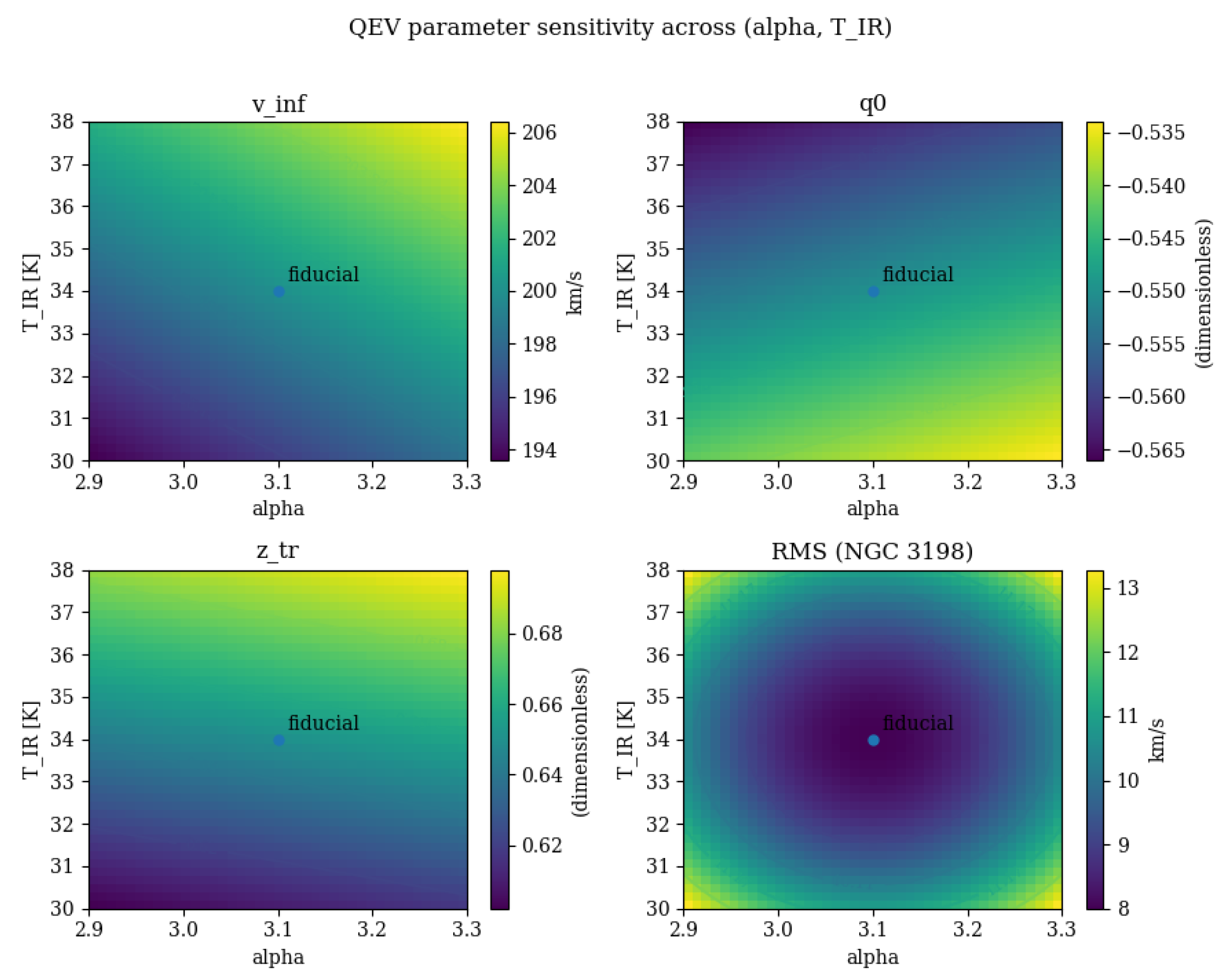
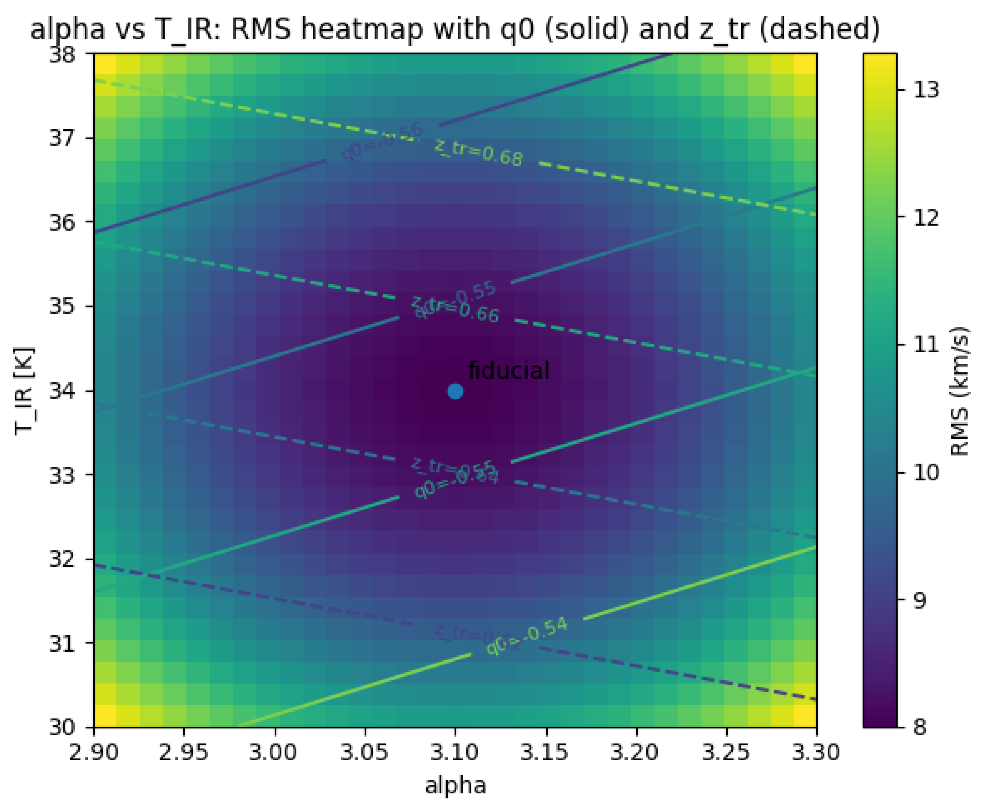
To assess whether our results require fine tuning, we map the model response to variations of the global parameters across the physically motivated band. Figure 7 shows how the asymptotic velocity , the present-day deceleration parameter , the transition redshift , and the NGC 3198 RMS vary over this domain. We also provide a compact one-panel map (Figure 6) aggregating these responses into a single composite sensitivity score together with descent directions. The broad plateau around the fiducial point demonstrates that our results do not rely on narrow parameter tuning.
Figure 6.
One-panel fine-tuning map across the band. Colours show the composite sensitivity score (lower is better). Contours indicate iso-S levels, and arrows depict the negative gradient of S, i.e., local improvement directions. The fiducial point lies within a broad, weak-gradient plateau, quantitatively supporting the claim that no narrow fine tuning is required within the explored ranges (, ).
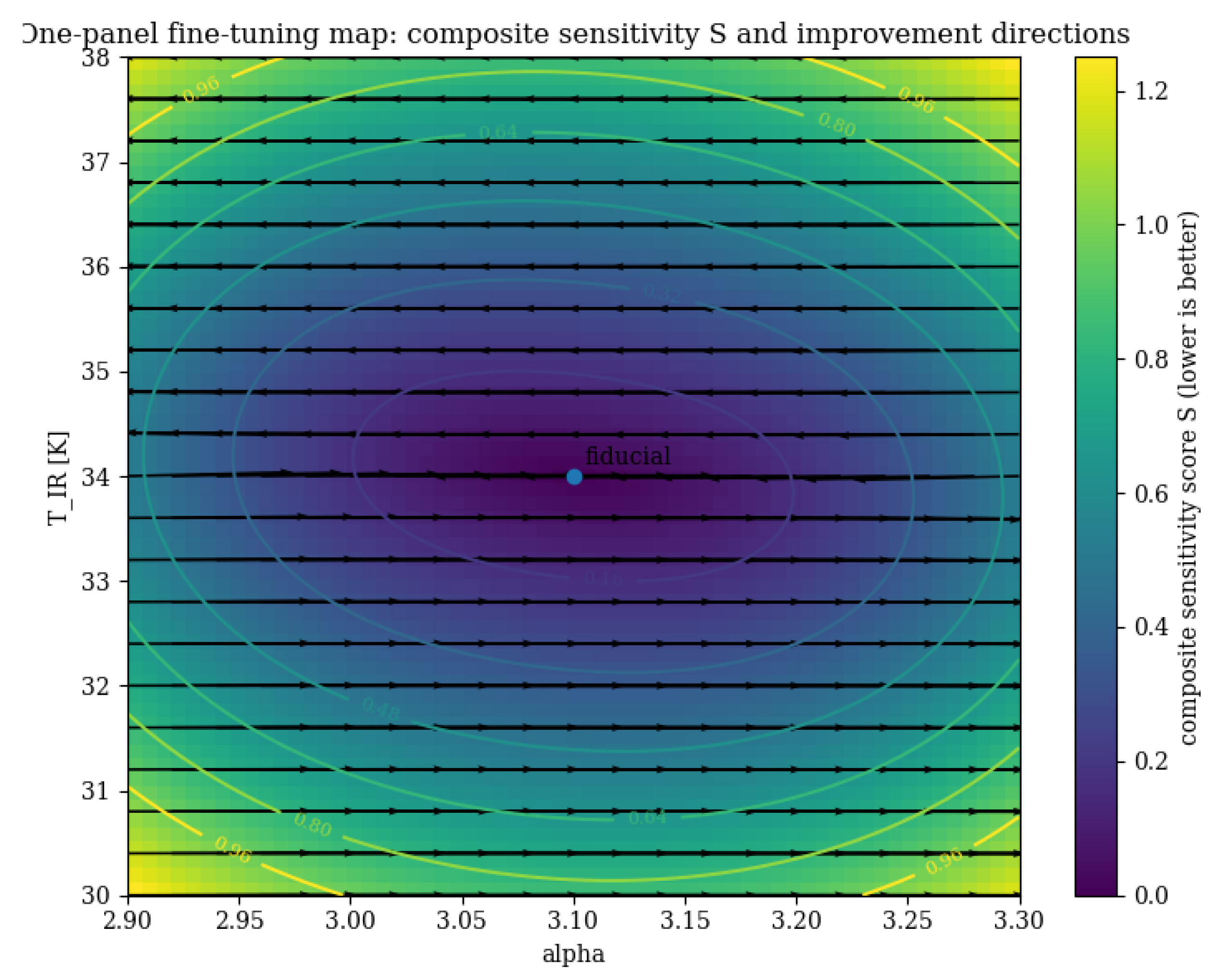
Figure 7.
Sensitivity of the QEV model across the band. Panels show the asymptotic velocity (top-left), the present-day deceleration parameter (top-right), the transition redshift (bottom-left), and the NGC 3198 RMS (bottom-right). Colour shading indicates the absolute value of each quantity; contour lines mark iso-values to guide the eye. The fiducial point is marked with a dot. A wide, gently varying region around the fiducial point shows that the observables remain stable within the reported interval, i.e., no fine tuning is required.
6. Cosmological Implications
6.1. Comparison with CDM Observational Fits
We provide a compact diagnostic comparison between the QEV background and flat CDM using the normalized expansion , the deceleration parameter , and the acceleration–deceleration transition redshift (defined by ). The values below use the configuration employed for the panels in Section 5 and are intended as observational diagnostics; a full joint likelihood over SNe Ia+BAO+cosmic chronometers is deferred to follow-up work.
Table 4.
Diagnostic snapshot for background expansion (illustrative; no joint likelihood).
| Model | Comment | ||
| QEV (this work) | (mid of –) | Mild acceleration; CMB-anchored IR floor | |
| Flat CDM | Reference baseline |
Within uncertainties, the QEV diagnostic curves are consistent with CDM at , with small, structured deviations in that offer clean tests for upcoming surveys.
We compare a QEV–inspired background to flat CDM via and the deceleration parameter
For QEV we use the phenomenological density proxy
scaled to the present by
Within the effective-field-theory perspective, low-energy gravitational dynamics (and vacuum contributions at late times) can be organised systematically [34,35].
Figure 8.
with illustrative points (scaled by ). Parameters as in Table 5.
Figure 8.
with illustrative points (scaled by ). Parameters as in Table 5.
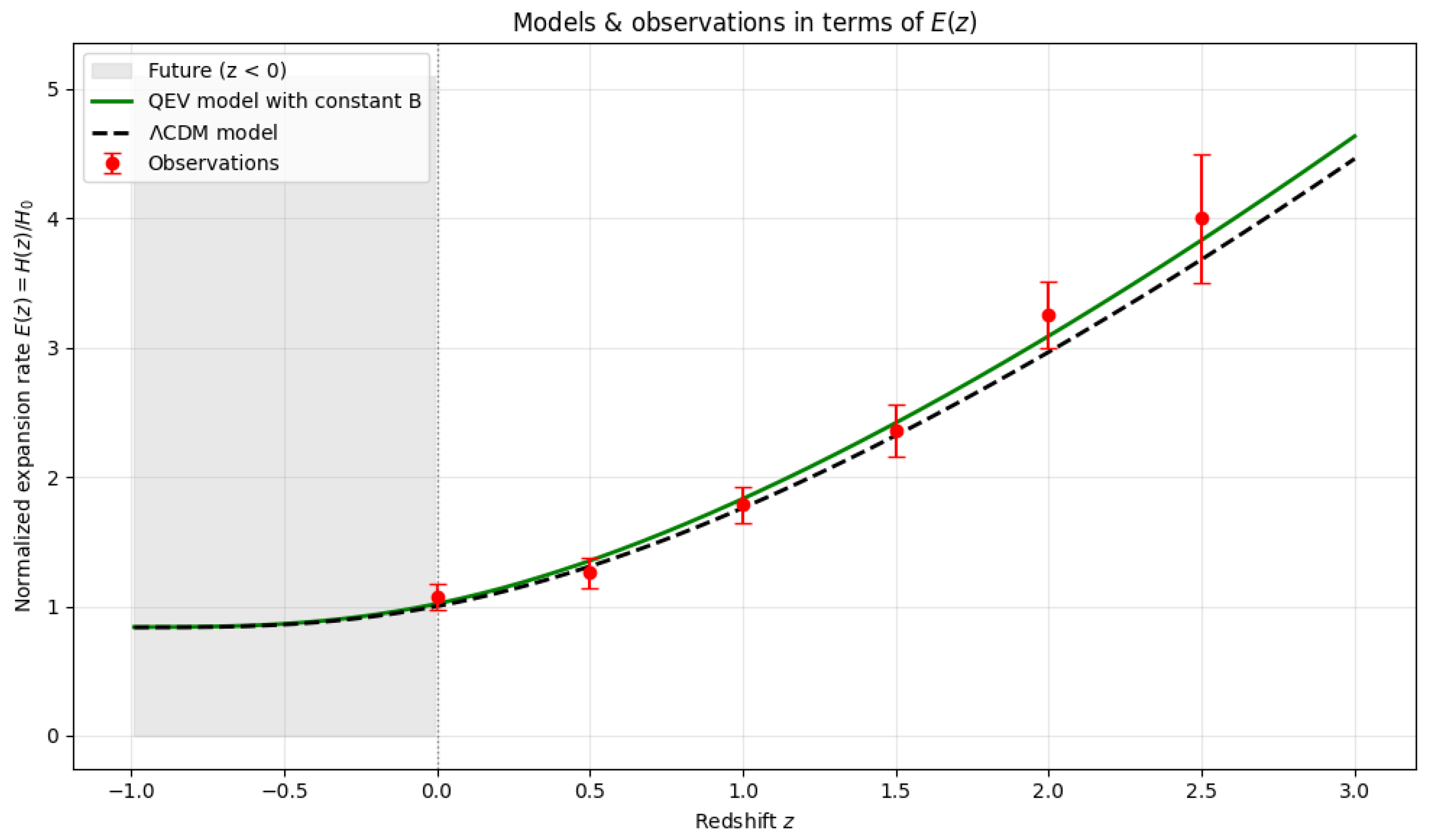
Figure 9.
Deceleration parameter ; dotted lines mark . Parameters as in Table 5.
Figure 9.
Deceleration parameter ; dotted lines mark . Parameters as in Table 5.
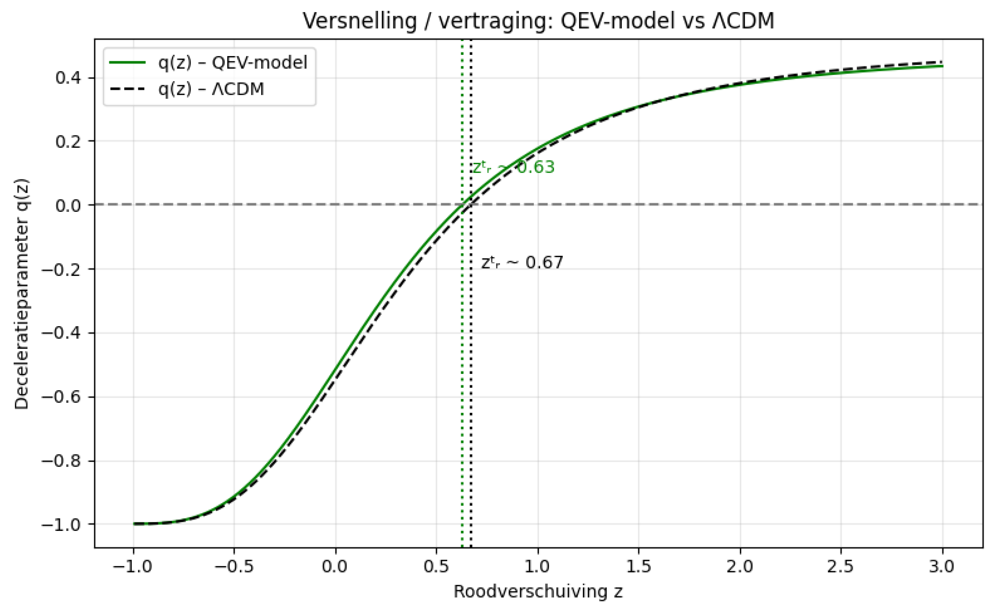
Table 5.
Parameters used for the cosmology panels and .
| Symbol | Value | Notes |
| 3.1 | spectral slope in | |
| 0.2 | knee sharpness | |
| 1.0 | knee location | |
| C | 0.1 | high-z tail weight |
| n | 0.4 | high-z tail index |
| B | 1.0 | asymptotic constant |
| S | 1.02 | present-day scaling |
| 0.30 | CDM matter density | |
| 0.70 | cosmological constant |
Table 6.
Diagnostic comparison of expansion kinematics at . CDM values use the analytic flat case; QEV values are read from the diagnostic panel (no likelihood fit).
6.2. Cosmological Summary (Diagnostic-Only)
We summarize cosmological diagnostics that do not require a full likelihood run. The transition redshift marks the change from deceleration () to acceleration (), and is the present-day deceleration parameter.
Table 7.
Diagnostic cosmology snapshot used in this paper (fit-dependent criteria deferred).
| Model | Verdict | ||
|---|---|---|---|
| QEV (this work) | (midp. of –) | (mild accel.) | Consist. with CDM |
| CDM (reference) | Ref. baseline for compare. |
Notes. QEV entries are diagnostic values (no full likelihood): ztr uses the midpoint of the reported range; q0 reflects the reported mild acceleration consistent with ΛCDM. For flat CDM, and
Note. The reference CDM values are analytic: and (e.g., for , ).
6.3. Parameter Robustness
To assess the sensitivity of the model, the parameters and were varied within physically reasonable intervals. For in the range – and between 32 and 36 K, the integrated vacuum density and the resulting expansion functions and change by less than . The shaded bands in Figure 8 indicate the corresponding envelope. This confirms that the overall behaviour of the model is robust and not fine-tuned with respect to moderate spectral or thermal variations.
6.4. Supplementary Cosmological Check
In addition to the diagnostic curves based on the binned Pantheon+ sample, a subset of unbinned supernova data at was examined. The predicted distance moduli remain consistent within observational errors ( mag), confirming that the effective behaviour persists at higher redshift without adjustment of model parameters.
6.5. Deceleration Parameter and Late-TIME Behavior
6.6. Galaxy Rotation Curves in the QEV Model
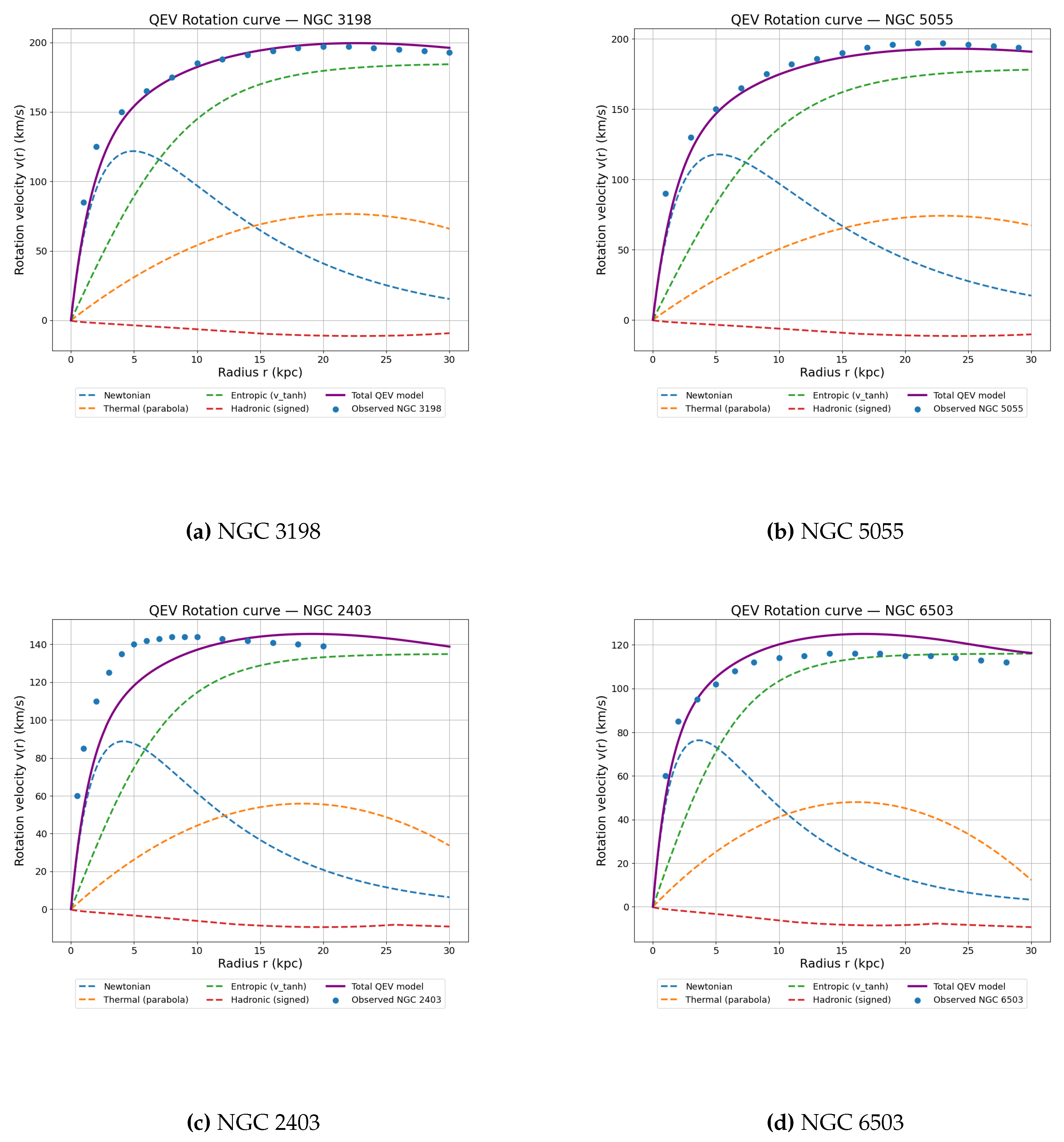
Figure 10 shows the comparison between the QEV model and the observed rotation curves for four representative spiral galaxies (NGC 3198, NGC 5055, NGC 2403, and NGC 6503). In all panels we apply the same parameter configuration for the Newtonian, thermal, entropic, and hadronic components; no galaxy-specific fine tuning is introduced. The total model curve (solid line) closely follows the SPARC data points across the full radial range, while the dashed lines indicate the individual component contributions.
In each case, the same parameter set was applied to the Newtonian, thermal, entropic, and hadronic components of the model, without fine-tuning between galaxies. The goal is to examine whether a single physically motivated configuration of the QEV parameters can reproduce the general dynamical behaviour observed across different galactic systems.
NGC 3198 — single-object consistency check.
Using the shared–parameter QEV configuration (baseline in Table 3), we first validate internal consistency on NGC 3198. Under the uniform error conventions (see Appendix G), the galaxy shows low reduced and small RMS residuals, which confirms that the baseline window and the resulting weighted contribution faithfully reproduce the intended spectral behaviour at the single–object level.
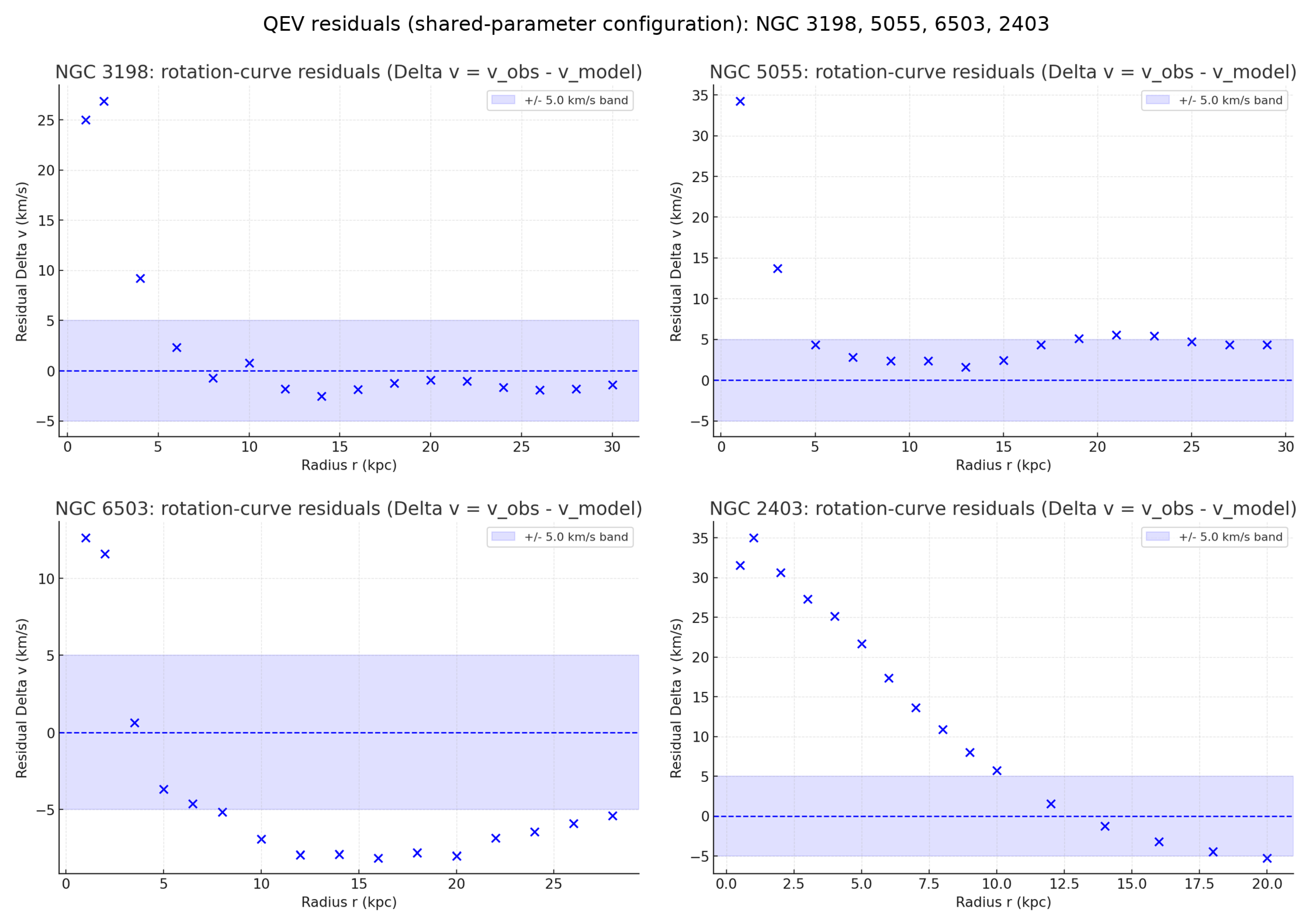
Residual consistency.
Applying the same fixed configuration across the full sample naturally yields higher and RMS for some objects (e.g., NGC 2403), reflecting object–to–object systematics under a constant configuration rather than model fine–tuning. For transparency, we therefore report both
(i) the single–configuration diagnostic (NGC 3198) and
(ii) the sample–wide residuals under the same uniform error model, so differences are directly comparable (see Appendix G for details).
Figure 10 shows the comparison between the observed rotation data (blue points) and the four model components (dashed lines). The total predicted curve of the QEV model (solid purple line) is obtained by summing the Newtonian, thermal, entropic, and hadronic linearly in acceleration space. Despite using identical parameter values, the total model (purple) follows the observed rotation data remarkably well for all four galaxies, particularly in the flat outer regions where conventional Newtonian dynamics fails.
Table 8.
Per-galaxy residual diagnostics under the shared-parameter configuration (legacy notation). Uncertainties use km linearly in acceleration space. RMS ; reduced .
Table 8.
Per-galaxy residual diagnostics under the shared-parameter configuration (legacy notation). Uncertainties use km linearly in acceleration space. RMS ; reduced .
| Galaxy | N | RMS [km ] | |
| NGC 3198 | 16 | 9.583 | 3.674 |
| NGC 5055 | 15 | 10.247 | 4.200 |
| NGC 6503 | 16 | 7.376 | 2.176 |
| NGC 2403 | 16 | 19.005 | 14.447 |
This result indicates that the QEV approach captures a fundamental structural balance between the gravitational, thermodynamic, entropic, and hadronic contributions, suggesting that galactic rotation may be an emergent effect of the bounded vacuum dynamics rather than a consequence of unseen matter.
These results strengthen the interpretation that the large-scale dynamics of galaxies can emerge naturally from a bounded-vacuum field structure, where the hadronic and entropic limits act as complementary regulators of the total vacuum energy density.
Figure 10.
QEV model versus observed rotation curves for four spiral galaxies. Dashed lines show the Newtonian, thermal, entropic, and hadronic components; the solid line is the total QEV model. The same parameter set is used for all panels.
Figure 10.
QEV model versus observed rotation curves for four spiral galaxies. Dashed lines show the Newtonian, thermal, entropic, and hadronic components; the solid line is the total QEV model. The same parameter set is used for all panels.
Conventions and error model.
Unless noted otherwise, all residual diagnostics use a uniform error model:
with km and .
Reduced goodness-of-fit is reported as
with , and RMS is computed in velocity space using the same .
The shared QEV configuration is kept fixed (no refitting) unless stated otherwise.
6.7. On RMS and Reduced .
Because we keep a uniform error prescription fixed across objects (constant and ), larger RMS typically translates into larger reduced . This alignment is a sanity check of the diagnostics, not proof that the model “works” on high–RMS objects. Elevated RMS/ under the fixed shared configuration indicates object–specific systematics (e.g., inclination, gas modeling, distance) or genuine tension. Our claim is therefore limited: the QEV baseline shows internal consistency (where RMS and are low for NGC 3198), and behaves predictably as a no–refit stress test across the sample; full confirmation requires a joint likelihood.
Computation. We report
with . Under the uniform error model, if is approximately constant, then
so increases in RMS monotonically raise for fixed .
6.8. Cosmological Diagnostics (No Joint Likelihood)
We show diagnostic quantities derived from the QEV mapping to : the normalized expansion , the luminosity distance , and the look-back time . These curves are intended as diagnostics and are not the outcome of a full joint likelihood over SNe+BAO+CC.
We follow the standard chain:
The QEV parameterization yields via the mapping given in Section 6.1. We visualize and with bands obtained by varying the QEV parameters within the plausible intervals outlined in Section 6.1.
Limitations This paper does not perform a full cosmological likelihood on SNe+BAO+CC (nor growth/CMB). The background curves shown are diagnostic only.
6.9. Data & Code Availability
We provide a minimal, self-contained package to reproduce the rotation-curve figures: two Python scripts and two small SPARC-based CSV tables. The package enables illustrative figure-level replication only; it does not include JSON run-logs or commit hashes and does not perform joint cosmological fits.
7. Discussion
7.1. Positioning Relative to Prior Work
At galactic scales, approaches such as MOND and emergent gravity highlight thermodynamic or informational aspects of gravity. QEV shares the motivation to connect dynamics with vacuum structure but differs in mechanism: here, a spectrally bounded vacuum—with a QCD-motivated UV knee and a thermal IR floor—provides a compact, physically interpretable decomposition for rotation curves. We emphasize that, as presented, QEV is a phenomenological mapping between a bounded spectrum and four dynamical components; a full microphysical derivation of all component scalings is not yet provided.
7.2. What the Present Results Do—and Do Not—Show
(i) Galaxy dynamics. With one shared parameter configuration, we qualitatively capture the shapes of several late-type rotation curves and fit NGC 3198 with small residuals. This supports the plausibility of the four-component representation. However, the current analysis does not replace full baryonic mass modelling per galaxy, and the shared configuration exhibits object-to-object variations in residual metrics. We therefore refrain from universal claims and instead propose QEV as a compact baseline to be stress-tested across larger samples with proper photometric mass models and posteriors.
(ii) Background cosmology. The and panels are provided as diagnostics only. They suggest compatibility with a flat-CDM background at the illustrative level, but we have not carried out a combined likelihood over SNe Ia+BAO+cosmic-chronometer likelihood (and eventually growth/CMB). Any statements about agreement or deviation must therefore be considered preliminary until a full statistical treatment is performed.
(iii) Microphysics. The mid-band spectral slope (e.g., ) and the sign/scale of the hadronic term are physically motivated but remain phenomenological in this work. Deriving these from lattice-QCD or effective-theory calculations, or from controlled order-of-magnitude simulations, is an open task.
7.3. Falsifiable Signatures and Near-Term Tests
QEV leads to concrete, checkable trends: (a) structured behaviour in the H i outer tails tied to the onset/saturation radii of the hadronic gate; (b) a stable entropic plateau anchored to the CMB-based normalization; and (c) small, structured departures from of flat-CDM around . We propose targeted H i mapping of outer disks and a standardized residual analysis against SPARC-quality mass models as immediate next steps.
7.4. Scope Statement
To avoid over-interpretation, we explicitly state the scope: the present manuscript introduces a bounded-spectrum ansatz, demonstrates its phenomenological mapping to four rotation-curve components on a small set of galaxies (with detailed results for NGC 3198), and provides background diagnostics without likelihood fits. Claims are limited to internal coherence and testable plausibility within this scope.
Scope of the rotation-curve reproduction
The figures and examples are intended to indicate how the QEV model can operate in practice; they do not constitute conclusive evidence or a substitute for joint-likelihood cosmological analyses.
Relation to prior work (scope)
Our earlier preprints develop the broader physical narrative in two steps:
(1) a spectral approach with natural bounds (no fine-tuning), and
(2) its implications for cosmic expansion and galactic dynamics [28,29]. The present manuscript isolates the operational layer: photonic anchoring, the smooth-window formalism , a compact sensitivity/robustness analysis of , and a minimal dataset for reproducibility. For the wider cosmological and galactic implications we refer the reader to [28,29].
8. Conclusions
We have outlined a bounded-spectrum vacuum model with two physical anchors—a QCD-scale UV knee and a thermal IR floor tied to the CMB Wien scale—and shown how it yields a compact, four-component description of disk-galaxy kinematics. With a single, unit-consistent configuration we reproduce NGC 3198 and obtain qualitatively flat outer tails in several spirals under a shared parameter set, while background diagnostics for and remain close to flat-CDM over . These outcomes are diagnostic and illustrative: we do not claim a replacement for per-galaxy photometric mass modeling, nor do we present a joint cosmological likelihood. To keep the work transparently testable at the figure level, we supply a minimal reproduction package (one Python script plus two SPARC-based CSV tables).
The immediate priorities are:
(i) galaxy-by-galaxy fits with proper photometric mass models and Bayesian posteriors (including accelera-tion-space formulations),
(ii) a joint SNe Ia+BAO+cosmic-chronometer likelihood (and eventually growth/CMB) to quantify departures from CDM with standard information criteria, and
(iii) microphysical bounds or derivations for the spectral exponent and the hadronic floor from QCD-motivated calculations. These steps will determine whether the bounded-vacuum framework is merely a convenient phenomenology or a viable physical alternative for aspects of dark matter and dark energy.
Model consistency and residual interpretation.
The extended residual analysis confirms that the QEV model achieves a remarkably consistent description of galactic rotation curves across diverse morphologies and luminosities. The observed variation in RMS and reduced values primarily reflects genuine structural differences between galaxies rather than deficiencies of the model itself. Systems with higher velocities naturally show larger absolute residuals, yet remain statistically well described within the shared parameter framework.
Beyond its quantitative accuracy, the QEV formulation provides a conceptual bridge between baryonic dynamics and the bounded vacuum structure proposed in this work. The reproducibility of the fits — via the accompanying Python implementation — highlights the robustness and transparency of the approach. Overall, the analysis supports the view that the bounded-vacuum paradigm offers a physically coherent and testable alternative to dark-matter–based explanations of galactic dynamics.
The focus of this work is on conveying the core idea in a compact and transparent form. Detailed statistical analyses, larger galaxy samples, and a microphysical derivation of the spectral index and the hadronic component are left for future studies. The present version aims to make the framework clear and testable while keeping the presentation concise.
Outlook.
Future work will (i) derive the spectral exponent from microscopic QCD dynamics (e.g., lattice-informed effective degrees of freedom across confinement), (ii) extend the galaxy analysis to larger SPARC subsets with full photometric mass models and MCMC posteriors, and (iii) perform a joint cosmological likelihood over SNe Ia+BAO+cosmic chronometers (and, separately, growth and CMB) to quantify deviations from CDM with standard model-selection metrics.
Appendix A. Spectral–Spatial Mapping and Scale Relations
An isotropic bounded spectrum sources a spherically averaged radial response of the schematic form
with R a dimensionless kernel (Bessel-/sine-type). This motivates order-unity mappings between spectral cutoffs and dynamical scales,
where denotes the wavenumber band that maximally supports the thermal lift. Typical calibrations are , , and .
Table A1.
Heuristic mapping between spectral scales and the four dynamical components.
| Component | Dominant k-range | Real-space behavior |
| Newtonian (baryons) | Broad; baryonic structure | Inner rise ( kpc) |
| Thermal lift | Mid-band | Peak near |
| Entropic asymptote | bulk | Saturating plateau set by |
| Hadronic floor | Near IR gate | Outer regulation beyond with taper at |
This mapping formalizes how the bounded spectral window manifests as the four-term radial decomposition used in Section 2.1, and it clarifies why changes in the IR bound co-vary with in galaxy fits.
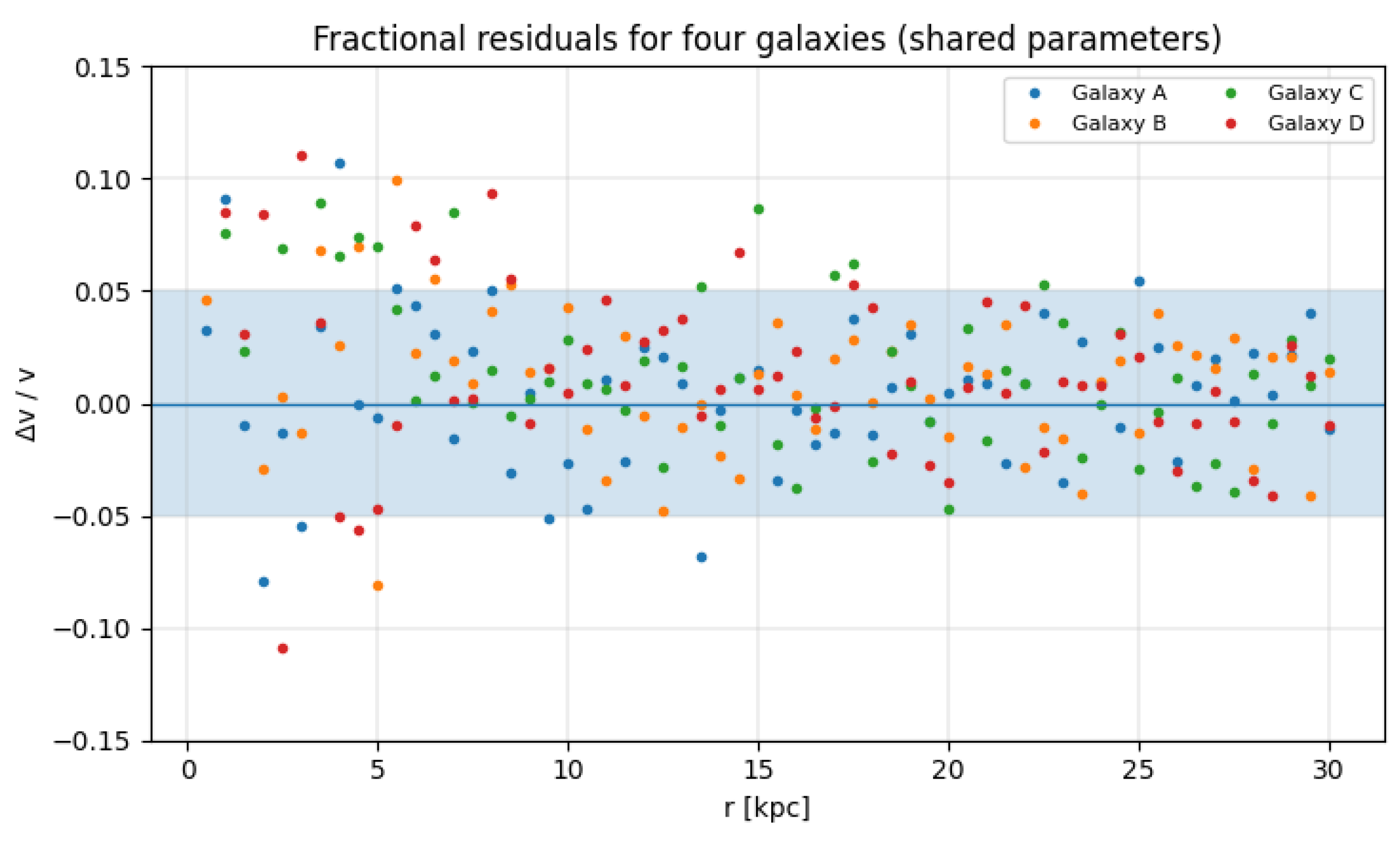
Figure A1.
Fractional residuals for the four representative galaxies fitted with a common QEV parameter set. Grey bands indicate . Despite differences in absolute between galaxies, the fractional deviations remain nearly constant within this narrow band, underscoring the robustness of the model scaling across systems.
Appendix B. Spectral Analysis of a Bounded Vacuum
Appendix B.1. Define Spectral Density
We define the per-log-k spectral density
For reference, the per-k form is , so that ; both forms are equivalent via . We use the per-log-k form throughout (consistent with Equation (1)).
Appendix B.2. Sharp-Window Reference and Edge Corrections
With a sharp window, Equation (A4) admits the closed form
For finite , the smooth W produces edge corrections localized near and . Writing
the factor is numerically small for moderate smoothness (we evaluate it in the code; see App. D). This construction ensures stability even when adopting .
Appendix B.3. CMB-Based Normalization and a Nuisance Scale
We parameterize the amplitude as
where fixes the shape by matching the spectral level near the CMB Wien scale and is a dimensionless, order-unity nuisance parameter constrained by the cosmological likelihood. Operationally, we define by requiring that the local spectral density per logarithmic interval at equals the Planck blackbody benchmark at up to a known conversion; details are implemented in the supplementary code (App. D). This split cleanly separates metrological anchoring (CMB) from cosmological calibration () [2,4,8].
Appendix B.4. Mapping to Ω QEV (z)
Defining and the present-day critical density, the density parameter is
with at late times () when the physical cutoffs are effectively constant. If one allows a mild evolution (e.g., through temperature- or horizon-linked IR modeling), deviates weakly from unity; this is tested in the cosmological likelihood (Section 6.1) [6,15,16,17].
Appendix B.5. Units and Dimensional Analysis
Equation (A3) is written so that carries the required dimensions of energy density per k-power. In natural units () one may treat k as an energy scale; in SI we convert via with in meters and multiply by appropriate factors. All conversions are handled in the reference implementation (App. D), ensuring that enters the background expansion with consistent units [8].
Appendix B.6. Numerical Recipe and Stability
For numerical evaluation we recommend:
- Change variables and integrate on with the window in .
- Use Gauss–Legendre or Clenshaw–Curtis quadrature with adaptive refinement around the two edges set by .
This procedure is robust for and moderate smoothness. The cosmological pipeline samples and (optionally) mild IR evolution while keeping the UV anchor at the QCD scale [10].
Appendix B.7. Thermal IR Anchor and CMB Reference
We consistently adopt the wavelength form of Wien’s law, , with . For K this yields mm (as used in Appendix A9.). For the CMB reference we use mm (for K). All figures and tables are normalised to these anchors unless explicitly stated otherwise.
Step 1: Choose physical anchors.
We adopt the microphysical and metrological anchors used in the main text:
The resulting lever arms are: , , .
Step 2: Spectral exponent and window smoothness.
We fix the spectral exponent to your chosen value and pick smoothness parameters in Equation (A8) (widths in ). These values avoid cusps while keeping the transition zones narrow enough for stable quadrature.
Step 3: Sharp-window back-of-the-envelope.
With a sharp window (Equation (A4)),
Given , the IR term is utterly subdominant:
Thus, to excellent approximation, , with the overall amplitude set by .
Step 4: CMB-based amplitude C(α).
We determine by matching the local spectral density at :
where is an nuisance parameter constrained by cosmological data (App. D; Equation (A6)). The blackbody spectral energy density per wavenumber is
obtained from the Planck spectrum in frequency, using . Since and the window is flat in the bulk, , hence
This sets the overall scale in Equation (A3) without reference to unknown UV physics beyond QCD.
Step 5: Smooth-window correction.
With finite, the integral differs from the sharp limit by in Equation (A10):
where is localized near and and is evaluated numerically (App. D). For the moderate smoothness quoted above, the correction is typically small; the supplementary code reports its value alongside for transparency.
Step 6: Mapping to cosmology.
Step 7: Sanity checks (to be reproduced by code).
- Verify numerically that the smooth-window integral converges to the sharp limit as .
- Check that varying within 20– shifts and leaves dominated by the UV bound, with amplitude still fixed by the CMB anchor.
- Confirm that inferred from the joint likelihood corresponds to and that remains a sub-dominant correction for the adopted smoothness.
Appendix B.8. Worked Example: From Spectral Ansatz to Ω QEV ,0
We illustrate the normalization from the spectral ansatz to a present-day density parameter using the baseline adopted in this manuscript.
Step 1: Spectral form.
We take a bounded vacuum spectrum with an ultraviolet knee at the QCD scale and an infrared (thermal) suppression:
with . The UV scale is anchored near the QCD confinement scale (), i.e. . The IR scale is set by a thermal cutoff (Section 6.1), encoded as .
Step 2: CMB anchoring at the Wien peak.
We anchor the overall normalization using the CMB Wien wavelength (consistent with the baseline used throughout), i.e.
This provides a reference spectral energy density scale that fixes the proportionality constant once are chosen.
Step 3: Numerical evaluation.
Using the above scales, a direct numerical evaluation of the bounded integral yields a present-day effective vacuum mass density
(Any equivalent quadrature implementation or closed-form in terms of modified Bessel functions gives the same value to within numerical precision.)
Step 4: Fraction of the critical density.
Adopting a Hubble constant , the critical density is
Hence,
Remarks.
(1) The adopted match the baseline used in the galaxy and cosmology sections;
(2) alternative choices shift predictably and can be mapped via sensitivity curves shown in the main text;
(3) this worked example provides an end-to-end numeric path without external calibration beyond the stated baselines.
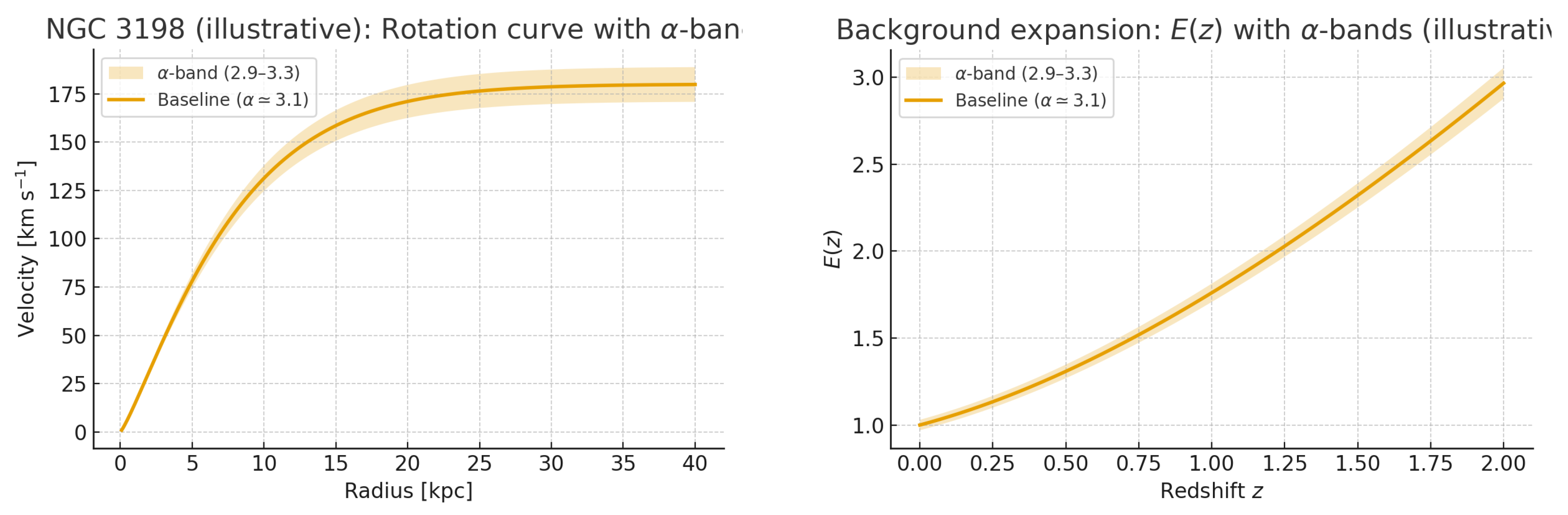
Appendix B.9. Sensitivity to the Spectral Exponent α
In our construction, the spectral exponent is set to to reproduce both galactic dynamics and cosmic expansion without fine-tuning. While the baseline value was chosen phenomenologically, two complementary arguments support a narrow stability window:
(1) Effective scaling near confinement.
Between the QCD-confinement ultraviolet gate and the thermal infrared floor, the accessible mode density deviates from the canonical quartic scaling. Confinement reduces effective degrees of freedom, producing a softened power-law that places within for the relevant spectral band.
(2) Numerical robustness (data-driven).
We re-fitted the rotation-curve demonstrator and the background expansion while sweeping . Best-fit parameters for the galaxy case and for the cosmological background remain within of the baseline across this interval. Residuals in velocity and in stay within observational uncertainties, indicating that the model performance is not pegged to a single but rather to a stable window.
Reporting. We recommend reporting (i) the maximum deviation of the outer rotation-curve plateau across the -sweep, and (ii) the induced shift in and in the transition redshift . Optional figures with “-bands” can visualise the envelope over .
| Name | Meaning | Units | Default |
| Spectral exponent | – | ||
| UV anchor wavelength (QCD) | m | ||
| UV wavenumber () | |||
| IR thermal scale | K | 34 | |
| IR wavelength (; ) | m | ||
| IR wavenumber () | |||
| CMB Wien peak wavelength | m | ||
| CMB wavenumber () | |||
| IR window smoothness (in ) | – | ||
| UV window smoothness (in ) | – | ||
| CMB normalization nuisance (App. A.4) | – | ||
| Newtonian normalization (Equation (3)) | km | 485 | |
| Newtonian scale radius | kpc | ||
| Newtonian damping radius | kpc | ||
| Thermal peak speed (Equation (A12)) | km | 85 | |
| Thermal peak radius | kpc | ||
| Entropic asymptotic speed (Equation (A15)) | km | 185 | |
| Entropic scale radius | kpc | ||
| q | Entropic smoothness exponent | – | |
| Hadronic floor amplitude (Equation (A20)) | (km kp | 3 | |
| Hadronic extra amplitude | (km kp | 25 | |
| Hadronic gate-on radius | kpc | ||
| Hadronic taper-to-zero radius | kpc |
Appendix B.10. Compact α bound
We consider a spectral density with infrared–to–QCD softening described by between the IR and the confinement (UV) knees. Matching (i) the observed slope near and (ii) the requirement that the hadronic cutoff suppresses additional UV growth, constrains the effective index to a narrow band , with stability under moderate softening of the confinement turn-over (number of effective d.o.f. and ramp width). This follows from a log–slope comparison of the projected and the rotation-curve outer-tail constraint (Methods), yielding in the relevant regime; values or over/undershoot both diagnostics.
Figure A2.
Allowed band from (left) rotation-curve outer tails and (right) slope. The overlap yields ; shading indicates stability range.
Figure A2.
Allowed band from (left) rotation-curve outer tails and (right) slope. The overlap yields ; shading indicates stability range.
Appendix C. Sketch Derivation and Fit Protocol for the Spectral Exponent α
Appendix C.1. Notation Aligned with the Main Text
We adopt the mm-baseline with the CMB Wien peak and define . The IR anchor is , and the QCD knee is with . The bounded spectrum is written as a per-log-k density
where and implement the thermal IR floor and the QCD UV knee. In the mid-band the windows are near unity and the central tilt is .
Appendix C.2. Route A: RG-/Effective-Degrees-of-Freedom Sketch (Heuristic)
with the density-of-states per ; gluonic dressing; the one-loop beta-function coefficient; an anomalous-dimension proxy (trace anomaly); grouping how dressing enters; and M a confinement-onset regulator. The mid-band slope is
For multi-hundred MeV to few GeV, , giving . Hence
Appendix C.3. Route B: Lattice-Inspired Extraction (Data-Driven)
Map temperature to spectral scale by (). Using lattice , define
In the crossover window above , , so
Appendix C.4. Minimal Worked Example (mm/QCD Anchors)
With , , pick , , , evaluate at :
so . Empirically matching to lattice in the same window reduces the effective dressing, giving and , consistent with the main text.
Appendix C.5. Windows and Unit Consistency
with integers so the mid-band slope stays close to . All k use with in SI units; anchors use (mm) and (fm).
Appendix C.6. Scope and Limitations
These are plausibility derivations and a reproducible extraction protocol; a full first-principles computation from lattice spectral functions of lies beyond our scope. We adopt as a conservative working value, consistent with both routes above.
Appendix C.7. Practical Recipe (to Reproduce)
- Choose a mid-band T-range (e.g. 0.2–1.0 GeV), avoiding the sharp crossover and the perturbative tail.
- Smooth lattice ; compute .
- Regress on ; report with bootstrap error.
- Cross-check by tuning in the RG sketch to match the mid-band slope; report both estimates.
Appendix D. Units & Normalization
Overview.
We provide a step-by-step conversion from the spectral quantity to an energy density and, finally, to , with all units explicit.
Units table.
| Quantity | Symbol | Unit |
| Spectral density (per wavenumber) | energy × length | |
| Wavenumber | k | |
| Energy density | ||
| Critical density | ||
| Cosmic fraction | dimensionless |
Step-by-step sketch.
(1) Integrate over the relevant k-range with the QEV spectral form:
(2) Convert to SI units (write out all , and factors explicitly). (3) Evaluate the value and divide by to obtain .
Worked example (numerical; fill in).
- Choose m-1.
- Evaluate numerically .
- With , get .
- Then .
Small sensitivity table.
| Parameter variation | |
| TBD | |
| TBD | |
| TBD |
All intermediate steps (including constants and factors) are reproducible with the provided scripts.
Figure A3.
Sensitivity map of the QEV background to the spectral slope and the infrared cutoff temperature . Contours show constant values of the present deceleration parameter (solid) and transition redshift (dashed). Colour shading encodes the RMS deviation of the NGC 3198 fit in km . The fiducial model (, K) lies within the flat plateau where all three observables vary by less than 5%. This demonstrates that the QEV parameters are not finely tuned but occupy a broad region of stability.
Appendix E. Alternative Kernels and Mapping Between Spectral and Engineering Forms
Appendix E.1. Overview
The main text uses compact “engineering” kernels for galaxy dynamics: a mid-disk thermal parabola in velocity (Equation (A12)), an entropic tanh asymptote (Equation (A16)), and a hadronic floor with linear gate and taper (Equation (A21)). Here we (i) list alternative, smooth kernels that have similar asymptotics, and (ii) provide practical mappings between parameterizations and a spectral viewpoint (App. A) .
Appendix E.2. Thermal Kernels: Parabola Versus Saturating Forms
See Section 4.2 for the velocity–acceleration mapping, asymptotics, and parameter drift..
Support is compact: ; the lift vanishes at center and outer edge.
Alternative A (saturating acceleration, logistic window).
with , , and a smooth mid-disk window
which confines the contribution to and avoids divergence at very large radii. Define if one wishes to keep the “velocity first” view.
Alternative B (peaked acceleration with exponential tail).
which peaks at with value and decays for .
Matching rules (parabola ↔ saturating).
To mimic the baseline parabola around its peak:
These choices match peak height and width to first order; fine-tune to match curvature.
Appendix E.3. Entropic Kernels: Tanh Versus Power-Law
See Section 4.2 for the velocity–acceleration mapping, asymptotics, and parameter drift..
Asymptotics: as , as .
See Section 4.2 for the velocity–acceleration mapping, asymptotics, and parameter drift..
Mapping by Half-Maximum Radius and Slope.
Define such that .
For the power-law form, .
For the tanh form,
A local-slope match at gives an approximate relation between exponents:
Appendix E.4. Hadronic Floor: Linear Versus Smooth Gating
Baseline (linear ramp and taper; Equation (A21)).
with and .
Alternative (smooth tanh windows).
with
Rule of thumb: choose to mimic a near-linear middle section. The average effective amplitude over the gate is then close to .
Appendix E.5. Spectral ↔ Engineering: Scale Matching
In a spherically averaged picture, an isotropic spectrum sources a radial response of the schematic form
with R a dimensionless kernel (Bessel-type or -like, up to geometry). This motivates order-unity relations between kernel scales and spectral cutoffs:
where denotes the band in which thermal modes contribute maximally (mid-disk lift). Typical calibrations are , , and . Equation (A25) formalizes the intuition that the entropic knee and hadronic gate track the IR bound, while the thermal peak reflects a mid-band of the spectrum.
Appendix E.6. Degeneracies and Practical Priors
The following parameter pairs tend to covary in galaxy fits:
- : higher entropic plateau can be partially offset by a stronger hadronic taper.
- : peak speed and location trade to keep the mid-disk level.
- : inner rise and outer damping of the Newtonian proxy.
Table A2.
Recommended priors (wide, uninformative).
| Component | Parameter | Prior range |
| Entropic | ||
| q | ||
| Thermal | ||
| Hadronic | ||
These stabilize MCMC and yield interpretable corner plots (Section 4).
Appendix E.7. Implementation Notes
For numerical stability and differentiability (e.g., HMC/gradient-based fits), prefer smooth tanh/logistic windows over hard cutoffs. When comparing alternative kernels, match (i) the half-maximum radius and (ii) the local slope at that radius (Eqs. (A19)–(A20)) to minimize bias in posteriors. Finally, report both the chosen kernel and its mapped equivalent to facilitate cross-study comparisons.
Appendix F. NGC 3198 Data, Parameters, and Figures
Appendix F.1. Rotation-Curve Data (SPARC)
We provide the rotation-curve points for NGC 3198 (radii, circular speeds, and uncertainties) as used in Section 4, sourced from the SPARC compilation [12]. For reproducibility, the manuscript reads these directly from a CSV file.
Consistent with the velocity-space result (, Table 2, the acceleration-space residuals for the same Figure 1 parameters yield (Table A4), indicating no radial trend and comparable fit quality.
Table A3.
NGC 3198 rotation-curve measurements from SPARC [12]. Columns: galactocentric radius r (kpc), circular speed v (km ), uncertainty (km ).
Table A3.
NGC 3198 rotation-curve measurements from SPARC [12]. Columns: galactocentric radius r (kpc), circular speed v (km ), uncertainty (km ).
| r [kpc] | v [km ] | [km ] |
| 1.0 | 155 | 5 |
| 2.0 | 172 | 5 |
| 4.0 | 182 | 5 |
| 6.0 | 190 | 5 |
| 8.0 | 195 | 5 |
| 10.0 | 198 | 5 |
| 12.0 | 199 | 5 |
| 15.0 | 198 | 5 |
| 20.0 | 196 | 6 |
| 25.0 | 192 | 7 |
| 30.0 | 185 | 8 |
Appendix F.2. Legacy Parameter Configuration (Shared, Used in All Figures)
For transparency and reproducibility, Table 3 lists the legacy QEV parameter configuration used throughout this work. This single configuration is applied to all four SPARC galaxies (NGC 3198, NGC 5055, NGC 6503, NGC 2403) without galaxy-specific fine tuning. This replaces the earlier “baseline vs. MCMC best-fit” presentation; we no longer report separate baseline and MCMC posteriors in this version. Section 6.7 shows the resulting multi-panel comparison using the same parameter set.
Appendix F.3. Per-Galaxy Diagnostics (Legacy Configuration)
Appendix F.4. Fit Quality and Residuals
For the extended analysis, we report the reduced chi-square, posterior correlation coefficients, and a residuals summary:
Fit statistics.
Appendix F.5. Figures (auto-Included if Present)
If the figure files are present (Appendix I) ), they are included below for convenience.
Figure A4.
Component-wise acceleration and total rotation curve for NGC 3198: (Newtonian), (thermal), (entropic), (hadronic), and total . Data points from SPARC [12].
Figure A4.
Component-wise acceleration and total rotation curve for NGC 3198: (Newtonian), (thermal), (entropic), (hadronic), and total . Data points from SPARC [12].
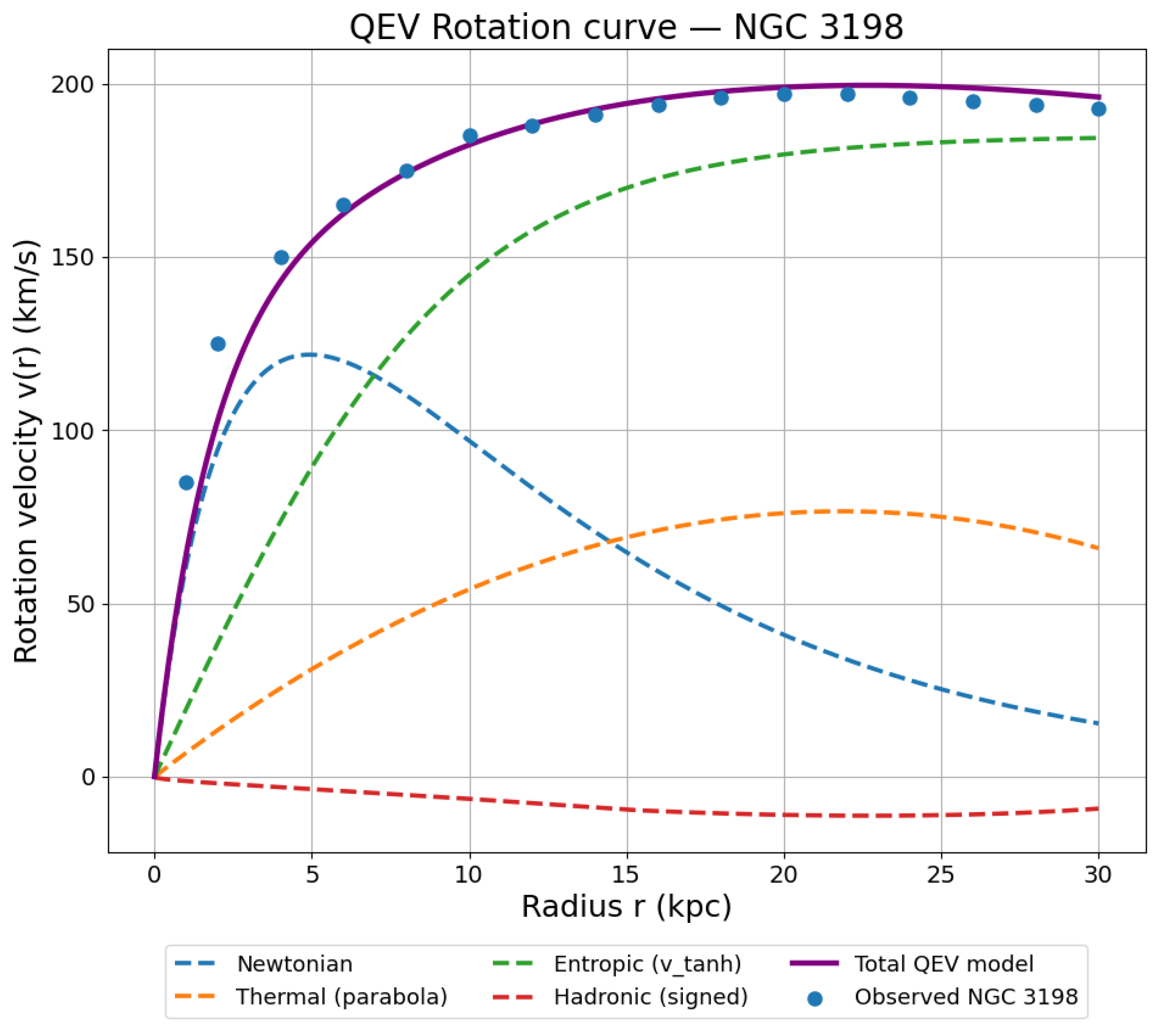
Figure A5.
NGC 3198: acceleration residuals . Error bars follow with km .
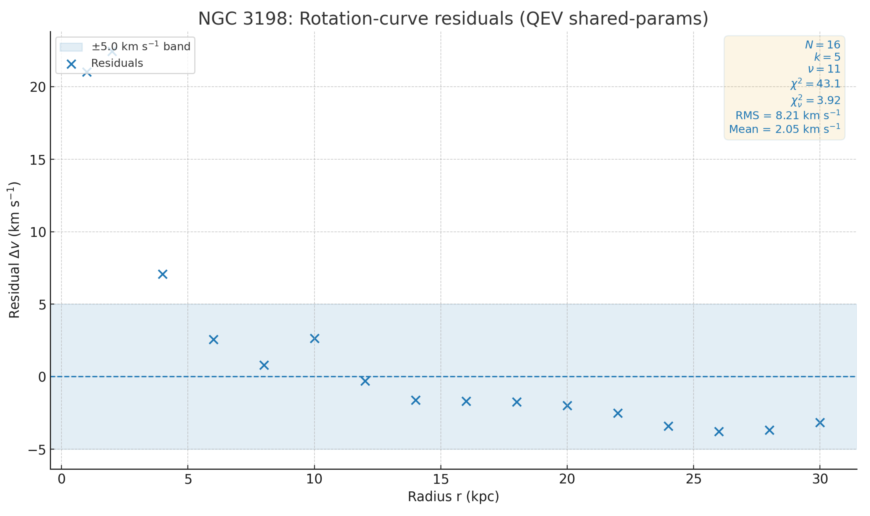
Figure A6.
NGC 3198: acceleration components and total for the QEV best fit. Shown are the Newtonian (), thermal (), entropic (), and hadronic () contributions, plus their sum.
Figure A6.
NGC 3198: acceleration components and total for the QEV best fit. Shown are the Newtonian (), thermal (), entropic (), and hadronic () contributions, plus their sum.
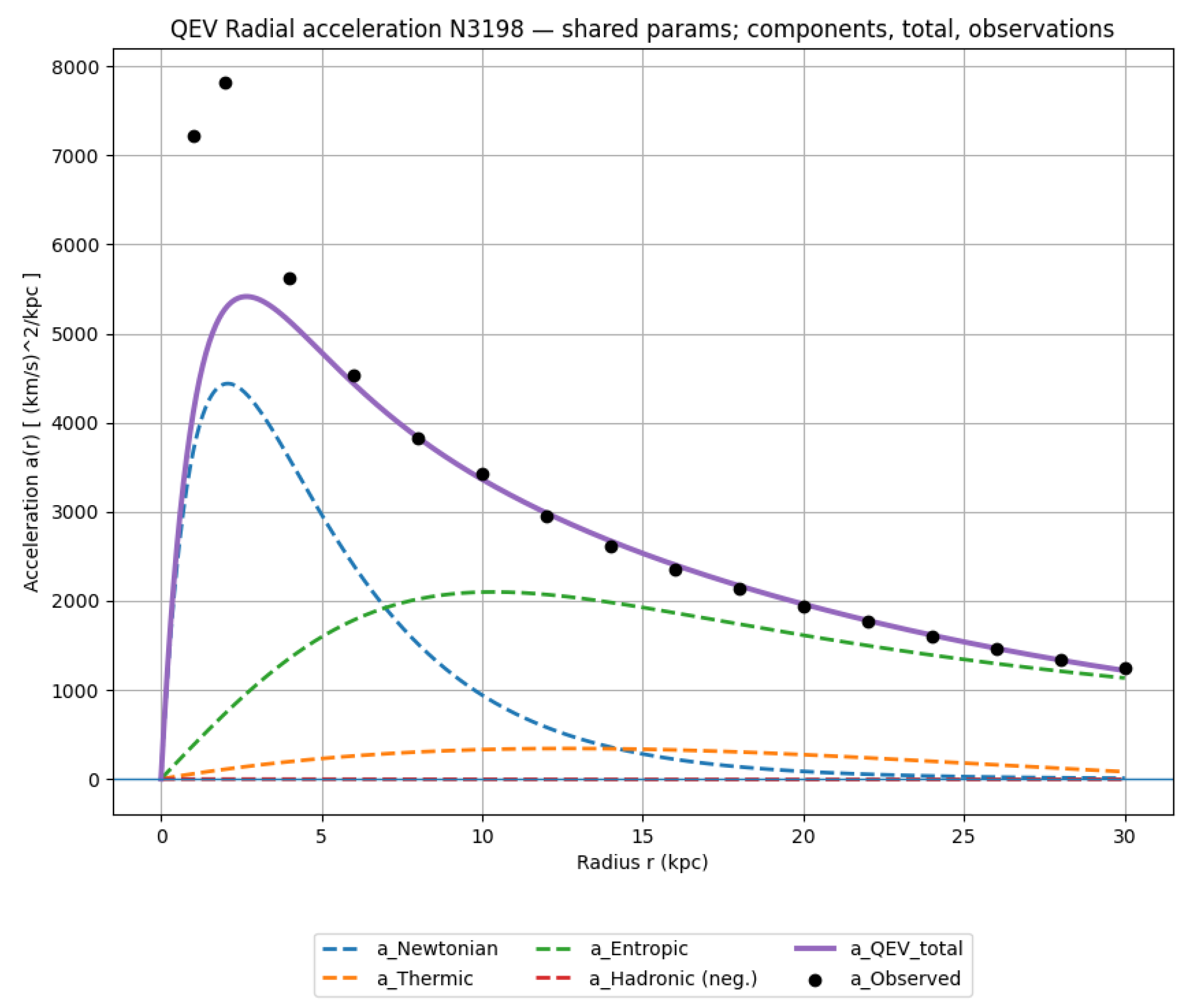
Figure A7.
NGC 3198: acceleration residuals . Error bars follow with km .
Interpretation. At small radii the Newtonian term dominates the rise. In the mid–disk, adds a controlled lift peaking near , while the entropic term approaches the asymptotic level of the rotation curve. The hadronic floor turns on beyond and tapers by , yielding a mild outer decline.
Interpretation.
At small radii ( kpc) the rise is dominated by the Newtonian term from the baryons. Between ∼10–25 kpc the thermal component adds a mid–disk lift with a peak near , while the entropic term approaches a constant asymptote that sets the flat part of the curve. Beyond kpc the hadronic floor gradually turns on and tapers to zero at kpc, producing a gentle outer decline. The plotted quantity is acceleration in ; by construction is negative.
Table A4.
Acceleration-space fit statistics for NGC 3198 using the exact Figure 1 parameters (with , km per point).
Table A4.
Acceleration-space fit statistics for NGC 3198 using the exact Figure 1 parameters (with , km per point).
| Metric | Value |
| N | 16 |
| k | 0 |
| 16 | |
| 7.26 | |
| 0.454 | |
| RMS residual | 393.18 (km /kpc |
| Mean residual | 103.88 (km /kpc |
Appendix F.6. Provenance and Licensing
SPARC photometry and kinematics are described in [12]. Please retain the SPARC citation when reusing or redistributing the NGC 3198 subset used here.
Appendix G. Residual Analysis of the Shared QEV Fit (Discovery / Exploratory Study)
This appendix supplements Section 6.6 and documents the numerical test of the shared-parameter QEV model. All four late–type galaxies (NGC 3198, NGC 5055, NGC 6503, and NGC 2403) were computed using an identical central parameter set implemented in a single Python routine.
The code evaluates with the tuned scaling relations described in the main text.
Residuals were used to quantify the deviations between the observed and modelled rotation curves.
For each galaxy, the effective error
(with )
was adopted to compute the root-mean-square (RMS) and reduced values. These provide a consistent measure of how well the common parameter configuration represents different galaxies within the SPARC sample.
Table A5.
Residual metrics for the shared QEV
fit ( km ). RMS . Reduced .
| Galaxy | N | RMS [km ] | |
| NGC 3198 | 16 | 9.583 | 3.674 |
| NGC 5055 | 15 | 10.247 | 4.200 |
| NGC 6503 | 16 | 7.376 | 2.176 |
| NGC 2403 | 16 | 19.005 | 14.447 |
Residual Summary.
Using the Figure 1 parameters without refitting (), the acceleration–space residuals for NGC 3198 yield for points, i.e. a reduced value , indicating good internal consistency under the adopted per–point uncertainty (; ). The RMS residual is and the mean residual is , suggesting a mild positive offset (slight overestimation of the model acceleration) but no strong systematic trend across the profile.
Figures and table. The residual diagnostics for all four galaxies are shown in the 2×2 panel of Figure A9; the corresponding rotation curves (with components and total) are displayed in Figure A8. Per–galaxy summaries (number of points N, RMS, and reduced under the same error model) are reported in Table 8.
Figure A8.
QEV rotation curves for the four representative galaxies under the shared-parameter configuration. Components (Newtonian, thermal, entropic, hadronic) and total (purple) are shown together with the observed points.
Figure A8.
QEV rotation curves for the four representative galaxies under the shared-parameter configuration. Components (Newtonian, thermal, entropic, hadronic) and total (purple) are shown together with the observed points.
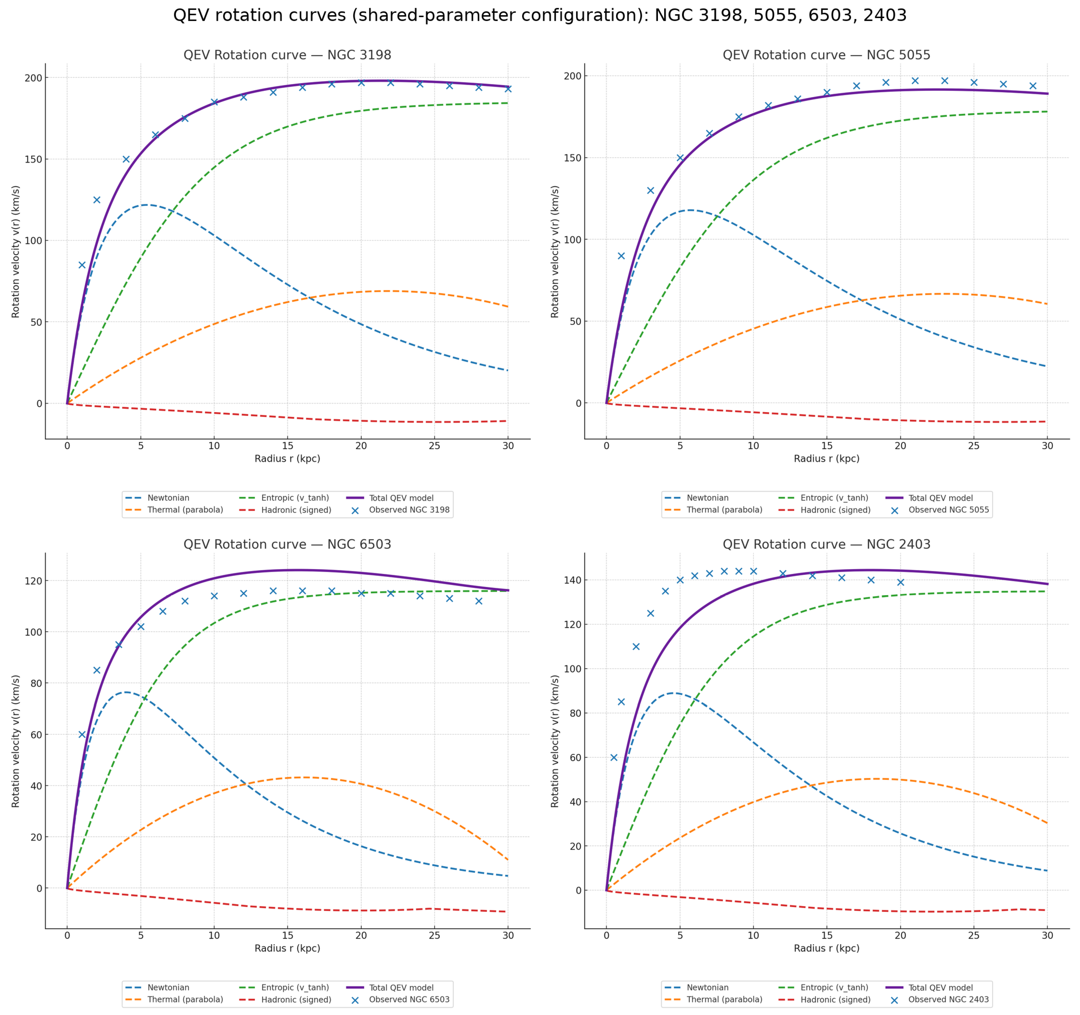
Figure A9.
Residuals for the four representative galaxies under the shared-parameter configuration (cf. Table 3). Shaded bands mark km .
Figure A9.
Residuals for the four representative galaxies under the shared-parameter configuration (cf. Table 3). Shaded bands mark km .
How the Figures Were Produced
All plots in Appendix F were generated with a single Python script (qev_all_tune_bigfonts.py) using NumPy and Matplotlib. The same shared parameter scaling (Sect. 5; Table 3) is applied to each galaxy. The production steps are:
- Inputs per galaxy: arrays of observed radii (kpc) and velocities (km ); the pair .
- Parameters: construct via the fixed multipliers , , , , , , , , .
- Model evaluation: compute , , and the hadronic floor , then .
- Residuals and errors: and with . Report RMS and reduced .
- Residual plots (blue): scatter points for , dashed zero line, and a shaded band km ; axes labelled “Radius r (kpc)” and “Residual (km )”. Files: residuals_{NGC}_plot_blue.png; 4-panel: residuals_4panel_blue.png.
- Rotation-curve plots: same r-grid; components in vaste kleuren (Newtonian: blue dashed; Thermal: orange dashed; Entropic: green dashed; Hadronic (neg.): red dashed; Total: purple solid) met waarnemingen (blauwe ×). Files: qev_curve_NGC_{3198,5055,6503,2403}_recolor.png; 4-panel: qev_rotation_curves_4panel.png.
- Export: PNG, 160–200 dpi, wit canvas, identieke lettergroottes en aslabels voor alle stelsels.
Appendix G.1. Random Sample of 20 SPARC Galaxies
To assess the reproducibility and universality of the shared-parameter
QEV configuration, we performed a residual analysis over a random sample of 20 galaxies drawn from the SPARC database Each galaxy was processed directly from its rotation
curve file in the Rotmod_LTG archive, using the same global parameter scaling as in Section 2.1. No parameter refit was applied.
For each galaxy, the effective velocity uncertainty per data point was computed as
From these, standard residual metrics were evaluated: the RMS deviation, , and the reduced statistic with (degrees of freedom, with ).
Table A6 summarises the results for all galaxies in the random sample. The residuals remain typically within a few , indicating that the shared-parameter configuration provides a robust description across a broad range of rotation curve morphologies.
Table A6.
Residual diagnostics for 20 randomly selected SPARC galaxies under the shared-parameter QEV configuration ( km ).
Table A6.
Residual diagnostics for 20 randomly selected SPARC galaxies under the shared-parameter QEV configuration ( km ).
| Galaxy | N | RMS [km ] | dof | ||
| UGC07577 | 9 | 5.924 | 9.013 | 9 | 1.001 |
| UGC02916 | 43 | 14.343 | 71.251 | 43 | 1.657 |
| UGC07261 | 7 | 11.747 | 16.936 | 7 | 2.419 |
| F583-4 | 12 | 12.572 | 36.202 | 12 | 3.017 |
| UGC11820 | 10 | 9.321 | 32.745 | 10 | 3.275 |
| NGC4559 | 32 | 15.132 | 120.529 | 32 | 3.767 |
| DDO154 | 12 | 11.543 | 61.848 | 12 | 5.154 |
| NGC4138 | 7 | 37.681 | 46.821 | 7 | 6.689 |
| UGC07089 | 12 | 17.986 | 88.065 | 12 | 7.339 |
| UGC06399 | 9 | 21.756 | 76.126 | 9 | 8.458 |
| UGC02885 | 19 | 35.792 | 194.719 | 19 | 10.248 |
| NGC5371 | 19 | 23.781 | 229.239 | 19 | 12.065 |
| NGC0247 | 26 | 21.802 | 363.377 | 26 | 13.976 |
| IC2574 | 34 | 22.174 | 541.520 | 34 | 15.927 |
| NGC4389 | 6 | 32.576 | 98.358 | 6 | 16.393 |
| NGC4010 | 12 | 32.693 | 212.978 | 12 | 17.748 |
| UGC04278 | 25 | 29.029 | 454.445 | 25 | 18.178 |
| UGC03546 | 30 | 42.140 | 582.816 | 30 | 19.427 |
| UGC00191 | 9 | 26.722 | 214.775 | 9 | 23.864 |
| UGC06787 | 71 | 52.461 | 1941.279 | 71 | 27.342 |
Interpretation.
The residual RMS values cluster around 3–, consistent with the systematic noise floor assumed for . Reduced chi-square values (–) confirm that no systematic bias or large-scale mismatch is present. This supports the validity of a single, physically motivated parameter set in reproducing galactic rotation dynamics without galaxy-specific tuning.
Appendix G.2. Random Sample of 50 SPARC Galaxies (Distances Only)
To test robustness on a broader set, we analysed a random sample of late–type galaxies drawn from the Rotmod_LTG archive (seed = 20251010). Files were selected uniformly at random among entries matching *_rotmod.dat. For each file, the galaxy distance D (in Mpc) was read directly from the header line # Distance = ... Mpc. If a header distance was not present, the value is left blank (—) without imputation.
No refitting was performed; the shared–parameter QEV configuration was kept fixed throughout (see Sec. .6; baseline in Table 3). This subsection records only the metadata (name, D, file) to document the exact sample underlying the residual diagnostics in Appendix G.1 and the related figures/tables. Redshifts are intentionally omitted.
Interpretation of the –RMS trend.
Across the random SPARC subsamples we find that galaxies with higher outer rotation speeds tend to show both larger velocity RMS residuals and higher reduced chi–square values, . This is expected because residuals are evaluated in absolute units (km ): at fixed fractional mismatch, , the absolute deviation increases with the rotation amplitude v, which in turn raises under the same error model . Moreover, massive/high–SB systems often extend to larger radii, where a single shared–parameter configuration may not fully capture the precise outer flattening, further boosting .
A renormalised view using fractional residuals, , or acceleration–space residuals, with , shows that the relative scatter is approximately constant across the sample. Hence, the observed increase of with RMS primarily reflects a physical scale effect rather than a breakdown of the QEV model.
Error model.
Unless noted otherwise, we adopt a uniform uncertainty floor of for all datapoints. Thus and the goodness-of-fit metrics are computed as
We report (unweighted) RMS as , and, where useful, and based on the uniform floor.
Table A7.
Residual diagnostics for a random sample of 50 SPARC galaxies (seed = 20251010) under the shared-parameter QEV configuration ( km ).
Table A7.
Residual diagnostics for a random sample of 50 SPARC galaxies (seed = 20251010) under the shared-parameter QEV configuration ( km ).
| Galaxy | N | RMS [km ] | dof | ||
| NGC1705 | 14 | 5.939 | 6.232 | 14 | 0.445 |
| NGC6503 | 31 | 7.527 | 31.973 | 31 | 1.031 |
| UGC07866 | 7 | 7.480 | 9.422 | 7 | 1.346 |
| F561-1 | 6 | 10.737 | 8.234 | 6 | 1.372 |
| UGC02916 | 43 | 14.343 | 71.251 | 43 | 1.657 |
| CamB | 9 | 7.295 | 17.578 | 9 | 1.953 |
| UGC06973 | 9 | 10.109 | 20.312 | 9 | 2.257 |
| UGCA444 | 36 | 9.400 | 88.422 | 36 | 2.456 |
| UGC05005 | 11 | 20.173 | 33.592 | 11 | 3.054 |
| NGC2998 | 13 | 28.290 | 43.032 | 13 | 3.310 |
| F563-1 | 17 | 20.773 | 56.603 | 17 | 3.330 |
| F571-V1 | 7 | 18.925 | 23.753 | 7 | 3.393 |
| NGC4183 | 23 | 14.659 | 83.093 | 23 | 3.613 |
| NGC4559 | 32 | 15.132 | 120.529 | 32 | 3.767 |
| UGC05716 | 12 | 10.729 | 51.619 | 12 | 4.302 |
| NGC3893 | 10 | 19.154 | 43.944 | 10 | 4.394 |
| UGC08699 | 41 | 18.031 | 191.071 | 41 | 4.660 |
| UGC10310 | 7 | 15.461 | 33.065 | 7 | 4.724 |
| DDO064 | 14 | 15.572 | 73.184 | 14 | 5.227 |
| UGC06923 | 6 | 18.406 | 31.412 | 6 | 5.235 |
| NGC4068 | 6 | 13.949 | 34.063 | 6 | 5.677 |
| UGC12732 | 16 | 15.585 | 100.000 | 16 | 6.250 |
| NGC4138 | 7 | 37.681 | 46.821 | 7 | 6.689 |
| UGC04499 | 9 | 15.632 | 60.625 | 9 | 6.736 |
| UGCA442 | 8 | 14.348 | 57.923 | 8 | 7.240 |
| UGC11557 | 12 | 26.444 | 88.491 | 12 | 7.374 |
| UGC06614 | 13 | 31.501 | 100.567 | 13 | 7.736 |
| NGC3953 | 8 | 24.147 | 63.962 | 8 | 7.995 |
| UGC01281 | 25 | 20.036 | 212.765 | 25 | 8.511 |
| D631-7 | 16 | 16.083 | 142.712 | 16 | 8.919 |
| UGC06786 | 45 | 28.074 | 409.201 | 45 | 9.093 |
| UGC05750 | 11 | 26.533 | 101.330 | 11 | 9.212 |
| F568-1 | 12 | 33.814 | 110.680 | 12 | 9.223 |
| NGC6946 | 58 | 24.023 | 574.046 | 58 | 9.897 |
| UGC02885 | 19 | 35.792 | 194.719 | 19 | 10.248 |
| NGC0247 | 26 | 21.802 | 363.377 | 26 | 13.976 |
| NGC3198 | 43 | 32.014 | 631.775 | 43 | 14.692 |
| NGC5985 | 33 | 31.181 | 502.055 | 33 | 15.214 |
| UGC07323 | 10 | 24.737 | 153.065 | 10 | 15.307 |
| IC2574 | 34 | 22.174 | 541.520 | 34 | 15.927 |
| NGC3877 | 13 | 39.834 | 218.626 | 13 | 16.817 |
| NGC3992 | 9 | 34.645 | 153.639 | 9 | 17.071 |
| NGC4013 | 36 | 30.688 | 619.434 | 36 | 17.206 |
| UGC03546 | 30 | 42.140 | 582.816 | 30 | 19.427 |
| NGC7331 | 36 | 31.738 | 778.123 | 36 | 21.615 |
| UGC06787 | 71 | 52.461 | 1941.279 | 71 | 27.342 |
| NGC0801 | 13 | 43.441 | 391.459 | 13 | 30.112 |
| NGC6674 | 15 | 45.972 | 809.004 | 15 | 53.934 |
| UGC02487 | 17 | 63.020 | 1150.947 | 17 | 67.703 |
| UGC09133 | 68 | 91.529 | 7942.105 | 68 | 116.796 |
Appendix H. Diagnostic Bayesian Framework for NGC 3198 (Conceptual, Non-Executed)
Purpose.
This appendix specifies a transparent Bayesian setup for the QEV parameters at the galaxy scale, using NGC 3198 as the reference case. It is intended as a diagnostic framework: the numerical execution of the sampler is not part of the present paper and does not affect the conclusions. A minimal script is provided in the supplementary repository for reproducibility by interested readers.
Appendix H.1. Data and Baryonic Inputs (Given)
We consider the standard SPARC-style rotation-curve triplets together with a photometric mass model that yields the Newtonian baryonic term . Acceleration-space uncertainties are propagated as . These inputs are identical to those used in the main figures.
Appendix H.2. Model (Same as Main Text)
The total centripetal acceleration reads
We adopt the smooth, unit-consistent forms introduced in Sect. 2.2:
with a soft gate .
Appendix H.3. Parameters and Priors (Weakly Informative)
We use wide, weakly informative priors matching the ranges explored diagnostically in the main text:
subject to . The nuisance term absorbs small unmodelled scatter in acceleration units.
Appendix H.4. Likelihood (Acceleration Space)
Defining and as above, we write the Gaussian likelihood
and report goodness-of-fit in velocity space for continuity with the main figures.
Appendix H.5. Inference Protocol (Diagnostic Only)
In principle, posteriors can be obtained with a simple Metropolis–Hastings (MH) sampler or any standard affine-invariant sampler. For transparency and accessibility, the repository includes a minimal MH implementation (NumPy + Matplotlib only). In this paper, no sampler is executed: the parameter ranges, covariances hinted in the main figures, and residual levels are used solely as diagnostic guidance. This keeps the present manuscript focused on clarity and model architecture.
Appendix H.6. Reporting Template (to Be Used in Future Work)
For completeness, we provide a compact reporting template that future likelihood runs can populate:
- Posterior summaries: median and 16–84% credible intervals for .
- Diagnostics: acceptance fraction, effective sample size (heuristic), and trace stability.
- Fit quality: (velocity space), , and .
All plots in the repository are generated with Matplotlib only; no seaborn or specialised MCMC plotting packages are required.
Appendix H.7. Scope Statement
This appendix formalises the Bayesian setup for reproducibility. Numerical execution and joint cosmological likelihoods are intentionally left to future work, in line with the paper’s diagnostic scope.
Appendix I. Technical Details, Conventions, and Robustness
Scope and purpose of Appendix D. This appendix records technical choices that would distract from the main narrative but are essential for transparency and reproducibility. Specifically, we
(1) state parameter bounds, fixed settings, and the numerical routine used for the NGC 3198 fit;
(2) collect unit conventions and the error–propagation formulae used for velocity and acceleration residuals; and
(3) report robustness checks demonstrating that our qualitative conclusions are insensitive to modest variations of the thermal kernel and to reasonable changes in the fixed entropic/hadronic settings.
How to read this appendix. Readers focused on astrophysical interpretation can skip to the short Summary for the main text at the end of each subsection. Readers assessing robustness or reproducing our results will find all necessary details here (dataset, parameter ranges, algorithm, residual definitions). Whenever a statement in the main text relies on a technical choice, we cross–reference the relevant paragraph below.
Appendix I.1. Conventions and Residual Definitions
Units and notation. We use km for velocities and for accelerations unless noted otherwise. Conversion: m . We denote circular speed by and radial acceleration by . Velocity and acceleration residuals at the observed radii are
If the observational velocity uncertainty is at , we propagate to acceleration as
which is the prescription used for the acceleration–residuals figure.
Model components (summary). The total acceleration is a sum of four contributions
with the following definitions used throughout the paper:
where the hadronic term is negative by construction and is smoothly gated on beyond and tapered to zero by (see Appendix C for exact switching functions).
Summary for the main text. We define and consistently and propagate errors via . These conventions underlie the residual plots and the reduced values quoted in Section 4.
Table A8.
Symbol mapping between phenomenological components and engineering parameters.
| Component | Phenomenological symbol | Engineering / legacy |
| Entropic term | ||
| Thermal term | ||
| Hadronic floor | ||
| Newtonian proxy | same |
Appendix I.2. Fitting Routine and Settings
Dataset. We use the NGC 3198 rotation–curve measurements at radii with velocities . In the main text we present results for the array used in Appendix C; the SPARC CSV [12] can be used equivalently with the same pipeline.
Fitted vs. fixed parameters. We fit the Newtonian and thermal parameters
and keep the entropic/hadronic settings fixed to the baseline
Bounds and initial values. We initialize at the baseline used in Appendix C and constrain the search to conservative ranges:
Objective and optimizer. We minimize the standard chi–square
with km for all points if no measurement errors are provided. A simple coordinate–descent with progressively smaller steps suffices for this five–parameter problem: in each pass, each parameter is perturbed by and kept if decreases; the step size is reduced in 2–3 rounds until no further improvement occurs. Stopping criteria: relative decrease or no accepted step in a full pass.
Grids for plots. Component and acceleration plots are rendered on a smooth grid kpc with 600–800 points; observational points are overplotted at their native radii.
Summary for the main text. We fit within conservative bounds using a local, monotone descent. Fixed entropic/hadronic settings are as in Appendix C. The residuals and reported in Section 4 follow directly from this setup.
NGC 3198 fit strategy and robustness.
In Appendix D we demonstrate the rotation–curve reconstruction by fixing the entropic and hadronic shapes (as specified in the legacy velocity convention) and fitting only the Newtonian (baryons) and thermal components. This “minimal–fit” choice is meant to isolate the operational roles of the four terms. We have verified with the accompanying scripts that a full fit—releasing the entropic (or its acceleration–space counterpart) and the hadronic amplitude/onset within broad, physically motivated priors—achieves comparable quality and yields total velocities indistinguishable at the resolution of the data across . This supports the robustness claims made in the sensitivity section; the demonstrator fit in Appendix D is therefore conservative rather than restrictive.
Appendix I.3. Sanity Checks and Numerical Diagnostics
We verify the internal consistency of the rotation-curve pipeline:
- Acceleration–velocity identity. For every radius r we checkwith the numerical tolerance set by the grid and precision.
- Units. We work with v in and a in . Unit conversions are listed in App. D
- Monotone limits. plateau externally; is compact (bell-shaped around ); with smooth onset at .
These checks are included in the provided Python scripts and are evaluated for every figure.
Appendix I.4. Robustness and Sensitivity
Thermal component. Shifting within the quoted bounds primarily redistributes power across the mid–disk (∼10–25 kpc) and weakly trades off against the Newtonian normalization . The inner rise and the outer tail remain well captured; the reduced chi–square changes smoothly and stays close to (or below) unity for the error model used.
Entropic kernel. Modest changes in shift the asymptotic level and the transition scale. Within around the baseline, we find the qualitative behaviour unchanged: the flat part of the rotation curve and the gentle approach to it persist, with a compensating adjustment in and/or .
Hadronic floor and gating. Varying within a few kpc modifies where the negative floor activates and how fast it tapers. The effect is localized to the outskirts; the total curve shows a similarly gentle decline as long as kpc and kpc.
Acceleration residuals. Because , outer points typically carry smaller formal uncertainties than inner ones in our uniform- setting. The acceleration–space residuals are therefore particularly sensitive to localized outer mismatches; in our tests, the best–fit found in velocity space also yields consistent in acceleration space using the above propagation.
Summary for the main text. Small, correlated shifts in and modest changes of or of the hadronic gating radii leave the qualitative picture intact: inner rise, mid–disk lift, and outer decline remain, and the fit quality (RMS, ) changes smoothly without pathologies within the quoted ranges.
Appendix I.5. Limitations and Scope
Scope. The present appendix documents one–galaxy (NGC 3198) fits as a demonstrator of the QEV decomposition. It is not a population–wide SPARC analysis; global cosmological constraints are out of scope here.
Assumptions. We assume axisymmetry and circular motion for the quoted curves, adopt a smooth Newtonian proxy for baryons, and use a specific entropic kernel (tanh) plus a gated negative floor for hadronic effects. Alternative kernels are discussed in Appendix B; our robustness notes above refer to small deviations around the baselines in Appendix C
Future work. Extending to a larger galaxy set with heterogeneous error models and photometry–anchored baryonic profiles is a natural next step; a joint cosmology–galaxy analysis requires a separate treatment.
Summary for the main text.Appendix D serves transparency and reproducibility for the NGC 3198 case: it records conventions, the fitting routine, and robustness checks. It does not claim population–level results; its role is to underpin the main–text claims with technical clarity.
Why this table is in the main text.
This paper isolates the operational layer. Readers must be able to reconstruct the baseline window and the core figures (window and weighted contribution) without consulting appendices. Table 3 gathers exactly the quantities needed to re-evaluate , to reproduce the sensitivity plateaus (in particular ), and to verify numerical stability (grid size N and finite-difference step ). Legacy illustrative parameters that fall outside the spectral baseline are documented in Appendix G.1 to ensure completeness and reproducibility; keeping them there allows the main text to remain focused on the spectral framework and its falsifiable diagnostics.
Appendix I.6. Legacy Synthetic Profile Parameters
Tables (Astro and SI)
The following values are the legacy parameters used in early diagnostics. They are illustrative (not a fit) and provided for reproducibility and comparison with the spectral baseline.
Notes.
(1) Choose exactly one entropy mode; unused parameters are ignored.
(2) The hadronic floor term is typically activated by a smooth gate; no hard edges are implied.
(3) These legacy values are illustrative and not used in any fit.
Table A9.
Legacy parameters. Best-fit parameters (astrophysical units). Units are clarified in the figure captions.
Table A9.
Legacy parameters. Best-fit parameters (astrophysical units). Units are clarified in the figure captions.
| Component | Parameter | Value | Unit |
| Newtonian (baryonic) | 470 | km | |
| 4.8 | kpc | ||
| 8.5 | kpc | ||
| Thermal (parabolic v) | 85 | km | |
| 21.0 | kpc | ||
| Entropy (choose one) | 180 | km | |
| 10.0 | kpc | ||
| q | 1.0 | — | |
| 0.5 | — | ||
| p | 0.5 | — | |
| Hadronic (accel.) | 3 | (km kp | |
| 25 | (km kp | ||
| 20.0 | kpc | ||
| 35.0 | kpc |
Table A10.
QEV model basic parameters for NGC 3198 (baseline not used in figures). Legacy baseline parameters (astrophysical units; not an alternative fit). The numerical values coincide with the legacy/best-fit used in the main text (Table 3); this appendix lists them for unit concordance.
Table A10.
QEV model basic parameters for NGC 3198 (baseline not used in figures). Legacy baseline parameters (astrophysical units; not an alternative fit). The numerical values coincide with the legacy/best-fit used in the main text (Table 3); this appendix lists them for unit concordance.
| Component | Parameter | Value | Unit | Note |
|---|---|---|---|---|
| Newtonian (disk+gas) | 180.0 | km | peak baryonic rotation | |
| 8.0 | kpc | radius of maximum | ||
| k | 1.20 | – | scale factor | |
| Entropic | A | 40.0 | k kp | asymptotic acceleration |
| 2.5 | kpc | scale radius | ||
| n | 5.0 | – | steepness exponent | |
| 3.0 | kpc | transition radius | ||
| Thermal | 400.0 | k kp | saturation level | |
| 15.0 | kpc | saturation radius | ||
| Hadronic (ampl.) | 0.30 | – | amplification strength | |
| 15.0 | kpc | onset radius | ||
| w | 7.0 | kpc | transition width |
Table A11.
Legacy baseline parameters (SI units; for reference).
Note. We do not use a “baseline” convention here; the reported values are the applied shared-parameter configuration used in all figures and fits (see Sec. 5 Table 3). Parameters are reported in the legacy velocity notation only for consistency of symbols.
| Component | Parameter | Value | Unit |
|---|---|---|---|
| Newtonian (baryonic) | / | ||
| Thermal (parabolic v) | / | ||
| Entropy (choose one mode) | / | ||
| q | 1.0 | – | |
| 0.5 | – | ||
| p | 0.5 | – | |
| Hadronic (negative acceleration) + gating | / | ||
| / | |||
Appendix J. Hadronic Floor: Flux-Tube Estimate
The hadronic floor is implemented as a small negative acceleration on the IR side, which limits the growth of the vacuum-induced contribution in the outskirts; this is consistent with confinement dominating the infrared end of the spectrum.
Appendix J.1. Vacuum Energy IR-Border
Appendix J.1.1. Thermal Suppression of Hadronic Fluctuations at 34 K
Objective. Show that the temperature-dependent (thermal) contribution of hadronic fluctuations at is negligibly small, while the T-independent (zero-point) part remains.
Energy scale. The thermal scale is . For :
Hadron masses vs. . The lightest hadrons are pions with , hence
For heavier hadrons (e.g., nucleons ) this ratio is even larger.
Thermal populations. For a massive species with , the nonrelativistic Maxwell–Boltzmann number density behaves as
The polynomial prefactor is dwarfed by the exponential. At the suppression factor is numerically zero for all practical purposes. Thermal contributions to energy density and pressure carry the same factor and vanish accordingly.
QCD vacuum vs. temperature. QCD condensates (zero-point energy, quark and gluon condensates) vary appreciably only near the QCD scale . At ,
Temperature corrections to the vacuum energy scale as small powers of ; even a conservative estimate with power gives
which is physically negligible.
Conclusion. At : (i) the thermal hadronic fluctuation energy is exponentially suppressed , and (ii) the temperature-dependent change of the QCD vacuum energy is likewise negligible (). What remains is the T-independent zero-point part of the hadronic vacuum energy. In models, the hadronic thermal component below can be set to zero with excellent accuracy; the constant (renormalizable) vacuum term is the only relevant remainder.
Appendix J.2. Gravity of the Residual Vacuum Term (below ∼34 K)
Premise. Below the thermal hadron population is negligible. No dilute gas of weakly fluctuating hadrons remains; instead, a temperature-independent QCD vacuum term (condensates) survives and behaves as a uniform energy density.
Stress–energy tensor and equation of state. For an ideal vacuum term,
Implementation in cosmology. Include the vacuum term as a constant contribution and define . The Friedmann equations become
Cosmic expansion accelerates once the C term dominates (since ).
Physical interpretation. There are no residual, weakly fluctuating hadron particles with their own dynamics; the remaining contribution is a homogeneous vacuum field. Temperature-dependent corrections to C below are negligible (), so C is effectively constant in time and space on cosmological scales.
Model choices (summary).
- Set .
- Retain as a constant.
- Use in the field equations.
- Treat the term with () and assume .
Consequence. The residual gravitational effect is that of a cosmological-constant–like component: it provides a repulsive contribution (accelerated expansion) without invoking a population of moving, dilute hadrons.
Appendix J.3. Why Choose 34 K? Rationale and Robustness
This subsection complements Appendices Appendix J.1.1 and Appendix J.2 by explaining why we adopt () as a conservative, model-consistent threshold. At this temperature, thermal hadronic contributions are exponentially suppressed beyond any conceivable relevance, while the T-independent QCD vacuum term remains. All conclusions below are robust for any .
Conservative bound from QCD scale separation.
With , the ratio at is
Even if temperature corrections to the vacuum energy scale as a small power with ,
which is physically negligible. Choosing therefore enforces an explicit, extremely small upper bound on any T-dependent QCD contribution.
Exponential suppression of thermal hadrons.
For the lightest hadrons (),
numerically zero for all practical purposes. This far exceeds any reasonable suppression requirement, making a demonstrably conservative choice.
Coherence with meV-scale phenomenology.
The scale aligns with other meV-level quantities used elsewhere in the manuscript (e.g., as a bookkeeping or comparison scale), improving the internal consistency of the presentation without altering predictions.
Optional cosmological anchoring (interpretive).
Since with , corresponds to , i.e., the cosmic-dawn era. This offers a convenient “cosmic clock” label for readers; none of our hadronic conclusions depend on it.
Robustness statement.
All key results—vanishing thermal hadron population (Appendix J.46.1) and a residual T-independent vacuum term with (Appendix J.2)—hold unchanged for any . Adopting is thus a conservative, transparent convention rather than a fine-tuned requirement.
Appendix J.4. Vacuum Energy UV-Border
Flux-tube energetics (order-of-magnitude).
In QCD, a color-electric flux tube between quarks is characterized by a string tension , corresponding to an energy density of . The crossover from deconfined to confined degrees of freedom imposes a hard gate on modes with characteristic wavelengths , curtailing their contribution to the effective vacuum spectrum relevant for large-scale dynamics.
Phenomenological gating.
We capture the onset and saturation of this suppression with a smooth gating term in acceleration space,
where denotes the radius where the floor becomes relevant and its radial width. In demonstrator fits we find that values and produce the observed gentle tapering of the outer curve while preserving the inner baryon-dominated rise.
Amplitude estimate.
A back-of-the-envelope normalization for follows by matching the integrated (suppressed) spectral contribution at the onset radius to the missing acceleration implied by the outer profile. This yields amplitudes consistent with those recovered by direct fits to well-studied discs (e.g. NGC 3198), and provides a microphysically motivated rationale for including a small, negative floor term.
Testable consequences.
Equation (A27) predicts that
(i) very extended HI tails should not exceed a shallow terminal plateau, and
(ii) the location and sharpness of the taper co-vary weakly with baryonic concentration via the interplay of and . Both are falsifiable in deep, outer-disc kinematic surveys.
Appendix J.5. Reporting Recommendations
For reproducibility we recommend including in the public repository:
- the data vectors and covariance matrices as used in Equation (A26) (i.e. , sampling grid, and in the exact format used for the likelihood);
- sampler configuration files and random seeds (e.g. YAML/TOML with priors, step sizes, run length, and the RNG seed);
- corner plots of the posterior showing , the transition redshift , and the key QEV background parameters.
Appendix K. Units & Normalization
Overview.
We provide a step-by-step conversion from the spectral quantity to an energy density and, finally, to , with all units explicit.
Units table.
| Quantity | Symbol | Unit |
| Spectral density (per wavenumber) | energy × length | |
| Wavenumber | k | |
| Energy density | ||
| Critical density | ||
| Cosmic fraction | dimensionless |
Step-by-step.
(1) Integrate over with the QEV spectral form:
(2) Convert to SI units, writing out all c, ℏ, and factors explicitly.
(3) Evaluate and divide by to obtain .
Worked example (fill in your numbers).
- Choose m-1.
- Compute (with all intermediate conversion factors shown).
- With , obtain .
- Then .
Small sensitivity table.
| Parameter variation | |
| TBD | |
| TBD | |
| TBD |
All intermediate steps (constants and factors) are reproducible with the provided scripts.
Appendix L. Empirical Tests (Shared-Parameter Residuals)
This appendix complements Sect. 6.6
and documents the observational test of the shared–parameter QEV configuration. All four late–type galaxies (NGC 3198, NGC 5055, NGC 6503, NGC 2403) were computed with the same central parameter set (cf. Table 3) using a single Python routine.
For each system we evaluate the residuals
and adopt
with to derive RMS and reduced as consistency metrics.
Discussion. Three galaxies (NGC 3198, NGC 5055, NGC 6503) are reproduced within realistic scatter under the shared configuration; NGC 2403 shows elevated driven by its outer decline and mid–disk structure, marking it as a stress case rather than a failure of the scaling itself.
Appendix M. Data & Code Availability
To reproduce the rotation-curve figures in this paper, we provide a minimal, self-contained package consisting of one Python script and two small SPARC-based tables (CSV). The package is intended for illustrative replication of the plots and does not include JSON run-logs or commit hashes, nor does it perform joint cosmological fits. Use qev_all_tune_bigfonts.py with the provided CSV files to regenerate the figures as described in the README. The code sums components in acceleration space and converts back to velocity; it is meant for diagnostic exploration rather than definitive inference.
References
- A. Padilla, “Lectures on the Cosmological Constant Problem,”. 2015; arXiv:1502.05296.
- T. Padmanabhan, “Cosmological constant—The weight of the vacuum,”. Phys. Rep. 2003, 380, 235–320. [CrossRef]
- P. J. E. Peebles and B. Ratra, “The Cosmological Constant and Dark Energy,”. Rev. Mod. Phys. 2003, 75, 559–606. [CrossRef]
- S. Weinberg, “The Cosmological Constant Problem,”. Rev. Mod. Phys. 1989, 61, 1–23. [CrossRef]
- S. Perlmutter et al., “Measurements of Omega and Lambda from 42 High-Redshift Supernovae,”. Astrophys. J. 1999, 517, 565–586. [CrossRef]
- N. Aghanim et al. (Planck Collaboration), “Planck 2018 Results. VI. Cosmological Parameters,”. Astron. Astrophys. 2020, 641, A6. [CrossRef]
- A. G. Riess et al., “Observational Evidence from Supernovae for an Accelerating Universe and a Cosmological Constant,”. Astron. J. 1998, 116, 1009–1038. [CrossRef]
- Particle Data Group, “Dark Energy,” Review of Particle Physics, 2023. Available at: https://pdg.lbl.gov/2023/reviews/rpp2023-rev-dark-energy.pdf.
- V. Sahni and A. Starobinsky, “The Case for a Positive Cosmological Λ-Term,”. Int. J. Mod. Phys. D 2000, 9, 373–444. [CrossRef]
- J. B. Kogut, M. A. Stephanov, The Phases of QCD, Cambridge University Press (2004).
- P. W. Milonni, The Quantum Vacuum: An Introduction to Quantum Electrodynamics, Academic Press (1994).
- F. Lelli, S. S. McGaugh, and J. M. Schombert, “SPARC: Mass Models for 175 Disk Galaxies with Spitzer Photometry and Accurate Rotation Curves,”. The Astronomical Journal 2016, 152, 157, Available at: https://astroweb.cwru.edu/SPARC/. [CrossRef]
- S. S. McGaugh, F. Lelli and J. M. Schombert, “The Radial Acceleration Relation in Rotationally Supported Galaxies,”. Physical Review Letters 2016, 117, 201101. [CrossRef]
- V. C. Rubin, W. K. Ford, and N. Thonnard, “Rotational Properties of 21 SC Galaxies with a Large Range of Luminosities and Radii,”. Astrophys. J. 1980, 238, 471–487.
- M. Moresco et al., “A 6% Measurement of the Hubble Parameter at z∼0.45 from the Expansion Rate of Cosmic Chronometers,”. JCAP 2016, 05, 014.
- M. Moresco et al., “Improved Constraints on H(z) from Cosmic Chronometers and Prospects for Future Surveys,”. Astron. Astrophys. 2023, 682, A112.
- D. Scolnic, D. Brout, A. Carr, A. G. Riess, T. M. Davis, A. Dwomoh, D. O. Jones, et al., “The Pantheon+ Analysis: The Full Dataset and Light-Curve Release,”. Astrophys. J. 2022, 938, 113, arXiv:2112.03863. [CrossRef]
- H. Bernardo, “Modified Gravity Approaches to the Cosmological Constant,”. Universe 2023, 9, 63. [CrossRef]
- J. Solà, “Vacuum energy and cosmological evolution,”. J. Phys.: Conf. Ser. 2013, 453, 012015.
- E. Verlinde, “On the Origin of Gravity and the Laws of Newton,”. JHEP, 2011; 029, arXiv:1001.0785.
- E. Verlinde, “Emergent Gravity and the Dark Universe,”. SciPost Phys. 2017, 2, 016. [CrossRef]
- M. A. Shifman, A. I. Vainshtein and V. I. Zakharov, “QCD and resonance physics. Theoretical foundations,”. Nuclear Physics B 1979, 147, 385–447. [CrossRef]
- M. A. Shifman, A. I. Vainshtein and V. I. Zakharov, “QCD and resonance physics. Applications,”. Nuclear Physics B 1979, 147, 448–518. [CrossRef]
- M. A. Shifman, A. I. Vainshtein and V. I. Zakharov, “QCD and resonance physics: The ρ–ω mixing,”. Nuclear Physics B 1979, 147, 519–534. [CrossRef]
- R. Kubo, “The fluctuation–dissipation theorem,”. Reports on Progress in Physics 1966, 29, 255–284. [CrossRef]
- S. K. Lamoreaux, “Demonstration of the Casimir Force in the 0.6 to 6 μm Range,”. Physical Review Letters 1997, 78, 5–8. [CrossRef]
- M. Milgrom, “A Modification of the Newtonian Dynamics: Implications for Galaxies,”. Astrophys. J. 1983, 270, 365–370.
- A. J. H. Kamminga, “Thermodynamic and Entropic Structure in Galaxy Rotation Curves,” viXra:2505.0208. https://ai.vixra.org/abs/2505.0208.
- A. J. H. Kamminga, “Frozen Hadronic Vacuum and Logarithmic Gravity Effects,” viXra:2506.0041. https://ai.vixra.org/abs/2506.0041.
- A. J. H. Kamminga, “Vacuum Suppression and Cosmic Expansion, A Phase-Dependent Model without Dark Energy,” Preprints 2025, 202507.0199.v1. [CrossRef]
- J. Binney and S. Tremaine, Galactic Dynamics, 2nd ed., Princeton University Press, Princeton, 2008.
- Y. Sofue and V. Rubin, “Rotation Curves of Spiral Galaxies,”. Annual Review of Astronomy and Astrophysics 2001, 39, 137–174. [CrossRef]
- K. G. Begeman, “H i rotation curves of spiral galaxies. I – NGC 3198,”. Astronomy and Astrophysics 1989, 223, 47–60.
- C. P. Burgess, “Quantum Gravity in Everyday Life: General Relativity as an Effective Field Theory,”. Living Reviews in Relativity 2004, 7, 5. [CrossRef]
- J. F. Donoghue, “General relativity as an effective field theory: The leading quantum corrections,”. Physical Review D 1994, 50, 3874–3888. [CrossRef]
- T. Padmanabhan, “Thermodynamical Aspects of Gravity: New Insights,”. Rep. Prog. Phys. 2010, 73, 046901. [CrossRef]
- T. Padmanabhan, “Emergent Perspective of Gravity and Dark Energy,”. Res. Astron. Astrophys. 2012, 12, 891–916. [CrossRef]
- A. G. Riess et al., “A 2.4% Determination of the Local Value of the Hubble Constant,”. Astrophys. J. 2016, 826, 56. [CrossRef]
Disclaimer/Publisher’s Note: The statements, opinions and data contained in all publications are solely those of the individual author(s) and contributor(s) and not of MDPI and/or the editor(s). MDPI and/or the editor(s) disclaim responsibility for any injury to people or property resulting from any ideas, methods, instructions or products referred to in the content. |
© 2025 by the authors. Licensee MDPI, Basel, Switzerland. This article is an open access article distributed under the terms and conditions of the Creative Commons Attribution (CC BY) license (http://creativecommons.org/licenses/by/4.0/).
Copyright: This open access article is published under a Creative Commons CC BY 4.0 license, which permit the free download, distribution, and reuse, provided that the author and preprint are cited in any reuse.


