
Submitted:
09 September 2025
Posted:
11 September 2025
You are already at the latest version
Abstract
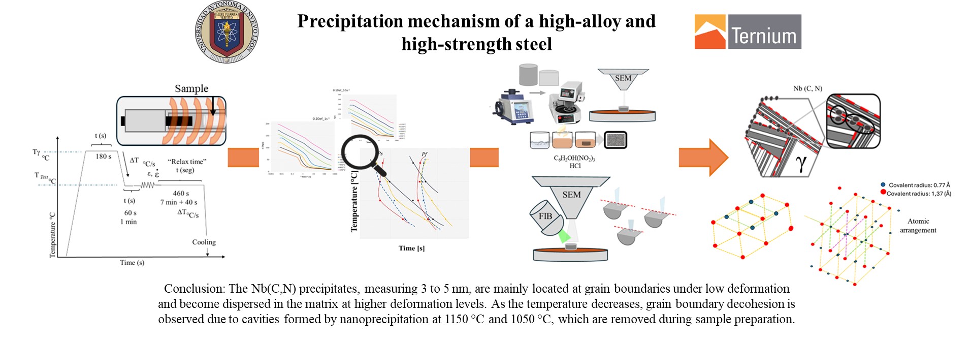
The thermomechanical process to obtain high alloy high strength steels is based on the control of variables such as temperature, deformation and strain rate to promote hardening mechanisms that directly influence the strength and toughness of the steel. Experimentally, it was determined for an API type steel, that the temperature of potential precipitation during the hot deformation process will be in a range of temperature from 1150°C to 1000°C. Precipitation will occur instantaneously due to temperature, deformation and strain rate (0.1 and 0.2 deformation and 0.5s-1 and 1s-1 strain rate) effect. The incorporation of microalloying elements as Nb in a percentage of < 0.050 significantly influences precipitation hardening preferentially located at austenitic grain boundaries. It was determined that precipitates of between 3 to 5 nanometers in size, distinguished as NbC will be obtained. It was found that the precipitation kinetics for the steel is affected by a single step deformation applied, by the formation of precipitate colonies at 0.1 deformation and strain rate 1s-1, which does not allow the dispersion of precipitates generating a planar interface in the microstructure of the steel. Finally, the preferentially localized precipitation mechanism of the almost continuous type by the grain boundaries was evidenced. This mechanism is crucial for controlling austenitic grain size during deformation, which leads to a final, homogenized microstructure.
Keywords:
thermomechanical processing
; precipitation kinetics
; API steels
; PPT diagrams
1. Introduction
The thermomechanical process for obtaining a high-alloy and high-strength steel is based on the control of process variables such as temperature (T), deformation (Ꜫ), strain rate(ε̇) and time (t). These variables allow the development of metallurgical phenomena that favor the properties of strength and toughness on the steel. The incorporation of microalloying elements in the chemical composition, such as the combination of Ti, Nb, Cr, Mo and Si, significantly influences the behavior of the alloy due to their impact on precipitation hardening and softening through the recrystallization process. The petroleum industry prompted the development of the HSLA (High Strength Low Alloy) steels family under the specifications of the American Petroleum Institute (API), used in the manufacture of hydrocarbon conductive pipes. These microalloyed steels are characterized as low-cost and high mechanical capacity [1]. Consequently, of this evolution, the need to improve strength and toughness of these materials, which led to the modification of their chemical composition specifications to meet market requirements. Generating the need to design and predict the behavior of steel, its mechanical properties and the control of the thermomechanical process, with the aim of optimizing its metallurgical characteristics [2].
Precipitation hardening in these steels can occur by solid solution or induced deformation. Figure 1 presents an illustrating diagram of the precipitation occurrence during the hot rolling process, where this mechanism can manifest itself in different stages: in the austenitic zone (γ), in the transformation austenite to ferrite (γ → α) or, finally, in ferrite (α) [3,4]. The development of materials with greater mechanical capacity and metallurgical reliability has led to the development of microalloyed steels through the incorporation of elements that improve the microstructure of the steel. Initially, it began with the addition of manganese (Mn) and, depending on its impact and market needs, other elements such as titanium (Ti), niobium (Nb) and vanadium (V) were integrated [1]. Elements that favor the formation of precipitates, such as Ti, Nb and V, to obtain compounds in the form of carbides, nitrides or carbonitrides. The formation of these compounds depends on the precipitation kinetics of the alloy, which, in turn, is determined by the applied thermomechanical process and the solubility of each element [5,6]. In the case of API grade steels, hardening by principates formation contributes significantly to improved strength and toughness. Therefore, the chemical composition modification is key in the development of high-alloy and high-strength steels, designed for the manufacture of hydrocarbon conductive pipes.
During the hot rolling process, temperature, deformation, strain rate and chemical composition influence the interaction between the hardening and softening mechanisms. The variation of these mechanisms is evidenced when, during precipitation hardening, there is a delay in the recrystallization of the microstructure. This generates changes in the non-recrystallization temperature due to the formation of compounds with elements such as Nb [7,8]. If temperature and strain conditions do not allow deformation-induced precipitation to progress, static recrystallization is triggered, resulting in the emergence of nucleation centers for the formation of new austenitic grains [9,10]. Finally, this research could be used to study the precipitation mechanism during the hot rolling process at an industrial level, with the purpose of understanding its impact on the properties of steel and optimizing its behavior for applications in the hydrocarbon industry.
2. Materials and Methods
For the study of the mechanism of deformation-induced precipitation, kinetics, interface sizes and morphologies in the steel during the thermomechanical process for a high alloy and high strength steel, a steel provided by the industrial sector was used.
Table 1 shows the experimental chemical composition of an API steel obtained using spark spectroscopy analysis under ASTM E415 [11]. The chemical composition is representative, but it corresponds to an API X60 grade.
From a transfer bar (deformed steel bar before the final rolling process) hot compression specimens of dimensions of 5mm x 10 mm, as shown in Figure 2, were machined in the longitudinal direction, which corresponds to the rolling direction. The equipment used for hot compression testing was the Bahr model DIL 805 A/D with this equipment is possible to control temperature, deformation, strain rate and cooling rate.
Once the strain was identified, hot compression tests with stress relaxation were performed using the thermomechanical cycle shown in Figure 3. The cylindrical samples were heated to an austenitization temperature, to obtain the previous austenitic grain size, and then cooled to the testing temperature at which the deformation took place, under 4 experimental conditions, using strain of 0.1 y 0.2 and strain rates of 0.5s-1 and 1s-1. The stress relaxation time was associated to the deformation process in a real industrial process. The cooling applied was quenched, to allow to maintain the microstructural characteristics generated by temperature, deformation and strain rate in the steel matrix.
The hot compression test with stress relaxation consists of subjecting the sample to compressive forces during the set time of 460 s, which was associated with the time that the industrial thermomechanical process lasts and which provides the slope that corresponds to the behavior of the microstructure due to the effect of the softening and hardening mechanisms that the steel presents due to the effect of temperature, deformation, strain rate and chemical composition.
Construction of Precipitation-Time-Temperature Diagrams (PTT)
From the stress relaxation curves, the negative slope generated was recognized, in which the softening of the steel and the start (Ps) and finish time (Pf) of precipitation were identified. This allowed the interaction between the softening and hardening mechanisms in the steel matrix to be identified. The experimental curves were analyzed as shown in Figure 4, identifying the formation of the plateau by the increase in stress, using Equation 1, that indicates the beginning and the finish of precipitation (Ps and Pf) during the stress relaxation until the slope is resumed [12,13].
Lastly, the time and temperature values for the construction of the PTT curves for the steel were collected from the detection of the increase in the stress on the slope.
Characterization of Deformation-Induced Precipitation
For the analysis of the microstructure of the deformed samples from the stress relaxation tests under the conditions of 0.1 and 0.2 strain and 0.5 and 1s-1 strain rate, the samples were subjected to conventional metallographic preparation with picric and hydrochloric acids used for the development of the deformed austenitic grain boundary. Optical microscopy (OM) analysis was performed to map the entire microstructure for the tested temperature conditions between 1150°C and 850°C.
Scanning electron microscopy analysis was incorporated using the JSM-IT300 LV–SEM equipment to obtain images of the areas of interest mapped by (OM) and images were obtained with secondary electrons (SE) and BED-S backscattered electrons to determine the mechanism of deformation-induced precipitation. For the identification of size, morphology and interface of the precipitates in the steel matrix, the transmission electron microscopy technique was incorporated using the JEOL JEM-2200FS -CS- TEM.
The Focused Ion Beam (FIB) technique was used for the preparation of the four conditions, 0.1 and 0.2 deformation and strain rates 0.5 and 1s-1 at 1050°C. For image analysis, editing, and magnification, ImageJ software was used to index diffraction patterns.
To achieve traceability, specimens were cut longitudinally and transversally, and SEM and TEM analysis were performed in the central area of the cross-face of the sample, as shown in Figure 5.
3. Results
Shown in Figure 6 are the softening curves obtained from the hot compression tests with stress relaxation, in which the slopes were marked to determine the start and finish times of the steel precipitation. The curves correspond to strain conditions 0.1 and 0.2, with strain rates of 0.5s-1 and 1s-1 tested at every 50°C, from 1150°C to 850°C. The softening slopes obtained do not present the characteristic behavior exhibited by the stress increase as precipitation occurs. Therefore, when identifying the change in the slope, it was determined that at temperatures below 1000°C, the slopes do not present a representative behavior of the plateaus that indicate precipitation, which does not indicate that it does not occur, but that under the experimentation window there was not time for the mechanism to occur at low temperatures [14,15].
It can be observed that, at temperatures between 1150 °C and 1000 °C, the behavior under all four conditions is similar and corresponds to the formation of a precipitation plateau with a steep or flat slope. This slope characteristic is associated with the delay in recrystallization due to the behavior of the steel during the hot deformation process. Because of temperature and deformation, there are oscillating hardening and softening mechanisms. The promotion of deformation-induced precipitation generates a delay in recrystallization, since there is no opportunity for nucleation centers or for the growth of new austenitic grains.
The temperatures where the slope changes due to the effects of increasing stress were identified, and the start (Ps) and end (Pf) points of precipitation were determined. The Ps and Pf results for each test condition and temperature are shown in Table 2. The steel precipitation kinetic curves were constructed from the data obtained in Table 2, considering only precipitation temperatures from 1150°C to 1000°C, Figure 7.
It was identified that precipitation kinetics, as a function of time and temperature, accelerates and occurs at high temperature, considering that the time for induced deformation precipitation to begin is less than 10 s. This is due to the rapid diffusion generated by the increase in dislocations and vacancies due to deformation, as atomic mobility increases locally, promoting almost instantaneous dynamic precipitation. It should be noted that precipitation kinetic curves do not present the typical “C” behavior, where the area of the of greatest precipitation is marked, because of the precipitation driving force and the diffusion process [14,15,16]. It was possible to identify that the condition that presents highest precipitation peak is the condition of 0.2 strain with 0.5 s-1 at a temperature of 1050°C, due to the high diffusivity it has due to temperature effects. This is attributed to the influence of alloying elements, the arrangement of the matrix due to deformation, as well as the addition of manganese, which is an element that delays the precipitation of niobium carbonitrides. It has been highlighted that the content of C and N are influential in the detection of the start and finish of precipitation, as well as the addition of Ti, which is characterized by a high solubility product producing a greater driving force of precipitation and which is also one of the elements with the possibility of nucleation in Nb (C, N) in addition to Si and Cr [17].
It should be noted that the temperature at which the precipitation curve begins is close to the dissolution temperature of the precipitate in the alloy. Considering that the curves under conditions of low deformation, in which the plateaus are flat and high temperature, the nose area is not completely distinguishable, this can be attributed to the size of the compound, the volumetric fraction and the distribution.
For the validation of the recrystallization delay of the experimental microstructure, of the stress relaxation tests specimens, the breakdown of the scans generated in the microstructure revealed by immersing the samples in the solution of picric acid and hydrochloric acid is presented, to identify signs of nucleation and grain growth that exhibit recrystallization. For all four conditions, at different temperatures between 1150°C and 850°C, there is evidence of the delay of the recrystallization mechanism during hot deformation, since there are no indications of nucleation centers and grain growth in the microstructure. It is recognized that the size and morphology of the austenitic grain does not present a significant deformation, which leads to the assume that the given deformation did not affect the initial morphology of the prior austenitic grain size. It was detected that as the temperature decreases, there is evidence of a thickening of the grain boundaries, which could be attributed to different factors such as the chemical etching capacity to reveal the grain boundary, the presence of a precipitation mechanism and the formation of an allotriomorphic ferrite [18], which is characteristic of high-alloy and high-strength steels.
The SEM images (Figure 8) show the typical mixture of martensite and bainite morphologies, a result of the quenching in each test. In the images, grain boundary areas are highlighted with red arrows, while yellow arrows highlight the areas where bainite transformation occurred with evidence of precipitation. Notably, for condition 2, with a strain of 0.1 and a strain rate of 1 s⁻¹ (Figure 9), cavities are observed within the original package, corresponding to the deformed austenitic grain.
This behavior can be attributed to the response of the microstructure to increasing strain rate and the generation of substructure packages within the original deformed austenitic grain package [19,20]. Therefore, the precipitation initially obtained and preferentially located at the grain boundaries, as shown in the condition shown in Figure 8, migrates to the substructure zones, recognized as substructure packages, due to the effect of deformation, strain rate, and temperature and time conditions.
The precipitation preferentially located within the substructure packages generated by the deformation, such as that shown in Figure 9 b) of the deformation condition 0.1 and 1 of the strain rate, are arranged in such a way that they could be colliding with each other, which favors the formation of larger cavities at the limits of the substructure packages. This behavior is shown in the diagram in Figure 10, which shows the evolution of the original package, which is the austenitic grain before deformation (a). Figure 10 b) shows the example of the formation of the substructure packages, marked with the red lines, and the preferential location of the precipitation that initially occurs at the grain boundary, and evolves as the deformation progresses, Figure 10 (c), until they end up colliding with each other forming cavities of greater dimension, they are not specifically the result of a single precipitate. The dependence of accumulated strain and strain rate on precipitation progression during the hot mechanical processing (hot rolling process) is highlighted.
In the images in Figure 11, condition 0.2 deformation and 0.5 strain rate, the precipitation behavior is repeated at the original deformed austenitic grain limit, with a completely homogeneous and consecutive distribution along the entire edge and identified by the red arrows in each of the micrography (a-h). This can be attributed to the deformation increase and dynamic precipitation that cause the appearance of deformation-induced precipitates at grain boundaries [21,22]. The yellow arrows identify areas of possible precipitation in the substructure, which favor the appearance of cavity zones due to the decohesion of the microstructure throughout the high-energy zone.
Figure 12 shows images of a condition of greater deformation and strain rate, in which an increase in the dimension of the cavities formed and preferentially distributed on the austenitic grain boundary is observed, perceived by the development by chemical attack that allows the transformation to be eliminated during the cooling of the samples for a better appreciation of the grain morphology and therefore, the identification of the location of the cavities. Where the existence of cavities without evidence of precipitation is attributed to the fact that during the metallographic sample preparation, the existing material was removed during the polishing process or was dissolved during the immersion of the sample in picric acid and hydrochloric acid for the development of the microstructure causing the decohesion of the material.
Figure 13 shows the deformed microstructure of the condition 0.1 deformation and 0.5 strain rate at temperature of 850°C by optical microscopy, in which areas around the grain boundary were observed to which the formation of a strain-induced ferrite was associated [22].
Figure 14 and Figure 15 show scanning electron microscopy with secondary and backscattered electrons under minimum and maximum strain conditions. They show that the areas near the grain boundary exhibit decohesion in the steel microstructure. Figure 14 shows grain boundary cohesion, which is attributed to the fact that this is a precipitate-free zone where, according to Figure 13, the possible formation of allotriomorphic ferrite at the grain boundary is observed.
Figure 15 shows the effect of 0.2 strain and 1s-1 strain rate at which there is the formation of preferentially localized cavities of the almost continuous type on the austenitic grain boundary, which are indicative of the mechanism of deformation-induced precipitation. This can be attributed to the chemical composition that includes elements that allow the formation of deformation induced precipitation of Nb, Cr, Mo and V [23,24,25], and present a behavior of preferentially locating at the austenitic grain limit, as shown in Figure 16, they coexist with the precipitate-free zones, therefore the zone in which deformation induced ferrite could be formed prematurely [26].
Measurement of the cavities shown in Figure 15, carried out with ImageJ software, show their size ranges from 0.5 to 2.5μm, as a result of the effect of the agglomeration of precipitates preferentially located at the limit of the deformed substructure.
From the point-to-point analysis obtained from the samples prepared for transmission microscopy, high-resolution STEM and TEM images of the four experimental conditions were obtained to demonstrate the deformation-induced precipitation mechanism. For the higher deformation and strain rate conditions, it was observed that the deformation-induced precipitation begins to concentrate in the form of colonies along the grain boundary, which supports the size of the cavities obtained by SEM, (Figure 14 and Figure 15) meaning that the size of the cavities preferentially located at the edge of the substructure does not correspond to the size of a single precipitate, but to the set of deformation-induced nano precipitates. Figure 17 presents the evidence of nanoprecipitate colonies preferentially located at the boundary of the substructure [27] due to the effect of deformation and the strain rate of 0.1 and 1s-1, marked with a yellow circle. Compared to condition 3, deformation 0.2 and strain rate 0.5s-1, it is observed that the precipitation mechanism presents the same precipitation preferentially located at the limits of the substructure.
Figure 18 a) shows the interaction of dislocations in the deformed substructure and deformation-induced precipitates, in which the arrangement and dispersion are the result of the thermomechanical process. In b) and c), evidence of the interaction and the area of dislocations, identified with the darkest areas in the sample, recognized as walls of dislocations [28]. From the microstructure shown in Figure 22, areas with indications of precipitation were selected to obtain dark field images. Figure 19 shows the morphology of a nanoprecipitate resulting from the analysis of condition 3 with the darkfield modality at a magnification of 5 nm. The morphology and size of a nanoprecipitate, compared to the nanoprecipitation in condition 2, exhibit a size between 3 and 5 nm, and are distributed in the steel matrix, generating a planar-type interface (Figure 18c)) due to the temperature effect and the increase in deformation that promotes nanoprecipitation in the steel matrix [29].
Figure 19 shows the width bands measurement that make up the nanoprecipitate fingerprint, which coincides with the covalent radius of the atoms that are approximately 0.1433nm ±0.01 in size, which coincides with the covalent radius of Nb that is distinguished by being 1.37 . This precipitation is characteristic of high alloy steels with elements such as Nb and Ti, typical elements for precipitating at high temperatures, which are in the steel matrix generating an interface related to the deformation and dislocations movement. The size and interface they present will influence the binding force of the austenitic grain boundaries to promote the hardening mechanism from grain refinement [30,31].
Figure 20 shows the result of increasing deformation at a temperature of 1050 °C, which by the effect of deformation generates a planar-type interface, with a coherent arrangement of the precipitates with respect to the matrix. In the STEM image, the morphology of the deformed substructure is not clearly visible, but the migration of precipitation from the grain boundary, in the lower left, to the matrix can be observed, which are responsible for the impact on resistance due to the coherent interface, spherical morphology and size in which they are found. The greater the deformation, the precipitation kinetics promote the volumetric fraction, the size and how they exist in the matrix [32,33].
Figure 21 shows the analysis of condition 4 in dark field mode, in which it can be seen in a) the nanoprecipitation distributed at the limit of the substructure, where the morphology and size coincide with those of condition 3, which range from 3 to 5 nanometers and with the prediction obtained with JMatPro of the size, as a function of time and temperature. Unlike the nanoprecipitates of condition 3, the measurement of the atomic radius is greater than the atomic radius of Nb, shown in b) and c). This can be attributed to the technique and the measurement accuracy, as well as the different alloying elements Ti, Nb, Cr and Mo, which promote nucleation and constitute the compound precipitates that were exhibited in the simulation study [34].
To conclude the validation of the formation of deformation-induced precipitation during the thermomechanical processing of steel, the results obtained from the electron diffraction analysis performed by transmission microscopy are presented.
Figure 22 shows the dark field image showing the areas where the electron diffraction analysis was performed. The image shows Z1, which corresponds to the boundary of the substructure generated by the deformation, and Z2, which corresponds to the area where the precipitation with coherent interface deformation induced was located in condition 2. This distinction of zones was made to identify the atomic order that characterizes the matrix and that which identifies the precipitate and its composition.
Figure 23 shows the result of analyzing the electron diffraction pattern (SAED) of zone 1 (Z1) exhibiting the diffraction points defined and distributed symmetrically as an oriented crystal structure, considering that steel has a BCC cubic structure, and the NbC precipitate is associated with an FCC crystal structure [33,34]. For the analysis of the electron diffraction pattern, the measurement was made from the point from the direct beam to each of the neighboring spots, shown in Figure 23 a). The measurements shown in Figure 23 b) were obtained, which correspond to according to the relationship , where R is the distance measured in nm-1. The assignment of the planes (hkl)was done by comparing the experimental values with the theoretical values reported for a typical crystal structure for NbC, which is recognized as FCC with a lattice parameter nm [35,36,37].
In Figure 23 c) a 3D model is presented that exposes symmetry according to the atomic arrangement of the unit cell of the crystal structure (FCC) for an NbC and in comparison with the points in the diffraction pattern, where the yellow and green dotted lines represent the edges of the fragment of a unit cell representative of an extended FCC crystal structure [38,39]. Where red dots represent the arrangement of Nb atoms and blue ones represent C atoms.
Table 3 shows the comparison of to which the candidate plane is associated by the approximation to the theoretical value. Showing that the diffraction pattern presents precipitates at the grain boundary associated with the crystal structure of NbC, where it coincides with planes (200) and (220), which presents a NaCl-type crystal structure with a lattice parameter of between 0.446–0.448nm. This lattice parameter can vary depending on temperature, processing, and chemical composition. It was identified that the experimental distances are associated with planes that would be forbidden for a pure FCC crystal structure, such as (210), (211), (310), but by comparison are the ones that coincide the most, this could be due to the presence of atoms at interstitial positions that allow the appearance of reflections, as well as to the participation of Ti, generating Ti-NbC, which are the ones with the greatest coincidence in the comparison of [36,37,38,39].
From these diffractions it was possible to recognize that in the diffraction pattern there is a diversity of assigned planes, and this may be due to the fact that the zone axis is not completely aligned with a high symmetry direction, additionally, in the sample there is an effect of deformation, defects that cause double diffraction, participation of other secondary phases, or residual stresses that modify the interplanar space [38,39]. To verify the association of the plans for an FCC structure, which recognizes the NbC, the NbC ICDD card (PDF 65-8782) was used. Where it is reported that for an NbC with a NaCl-like structure with space group Fm-3m, with the following values , etc [40,41,42].
Figure 24a) shows the result of analyzing the electron diffraction pattern (SAED) of zone 2 (Z2) that shows the measurement from the origin point to the diffraction points, in the same way done for Z1. Figure 24 b) shows the distances and obtained distance to identify the characteristic plane of each diffraction associated with an FCC crystal structure, considering a characteristic lattice parameter of NbC, . Figure 24 c) shows the 3D model that exhibits the symmetry considering the atomic arrangement for a FCC structure, created by the yellow lines that represent the edges of the cubic cell and the green and purple lines the location of Nb on the faces, identified with the red dots. Where C atoms, represented by blue dots, exhibit accommodation in the octahedral interstices in the NbC arrangement FCC, like the typical structure of NaCl [36,37,38,39], in which C is surrounded by 6 Nb atoms placed at the vertices and on the faces.
Table 4 shows the comparison between theoretical and experimental, considering the lattice parameter typical of NbC [40,41,42,43]. Allowed planes for FCC were identified, such as (220), (444), (622) and (620), which match the structure of the NbC. It was identified that the measurement from the center to the furthest points coincides with the high-order planes (444), (622) and (620), which are the planes furthest from the center, which in the case of the plane (220) is a low-order plane and is recognized as reflection close to the center, in both cases these are planes associated with reflections allowed for FCC, for meeting the Miller indices condition (hkl), and which also in agreement with the information reported on the card for the NbC, ICDD (PDF 65-8782) [44,45,46]. In the comparative analysis of the distances , the difference was calculated and reported. It was observed that point 7 with a 0.1704, associated with the plane (220), shows a difference of 7.78%, which can be associated with the measurement method due to the precision when assigning the distance when drawing the line in the diffraction pattern. However, most distances have a difference of less than 4%, which supports that diffraction analysis is acceptable [44,45].
Therefore, from the electron diffraction patterns analysis, it is considered that the precipitates induced by deformation in the steel are NbC type with FCC crystal structure. These are initially located at the grain boundaries (zone 1), which due to the effect of deformation and the arrangement and appearance of new surfaces, migrate to the matrix (zone 2) to generate a coherent planar interface, which will allow determining the precipitation mechanism of NbC induced by deformation.
Based on the results from the microstructural characterization by scanning electron microscopy (SEM), the identification of the preferentially localized precipitation, the validation of such precipitation in the substructure of the deformed microstructure by backscattered electron diffraction (EBSD), and the analysis of the interface between the precipitates and the matrix in high-energy areas, Figure 25 shows the distinctive mechanism of the steel is precipitation in austenite with a localized distribution, which presents a coherent interface with the matrix [22,29].
Evidence shows that precipitates are located at grain boundaries due to experimentally induced deformation. As the deformation process progresses in the microstructure of the steel, a localized distribution was characterized that arises in the microstructure of the material from the segregation of carbon, nitrogen and niobium atoms. These elements are primarily responsible for forming complex compounds such as niobium carbonitrides (Nb(C, N)) during the hot deformation process [32,42,43,44,45,46,47,48].
MEB characterization allowed to observe the formation of cavities typical of decohesion in grain boundaries, caused by the presence of deformation induced precipitates. The size of the cavities observed in the samples characterized by MEB did not correspond to the typical size of nanoprecipitates identified by transmission microscopy, but they are colonies of nanoprecipitates between 3 and 5 nm in size.
Experimental conditions, specifically temperature, deformation and strain rate, limited the dispersion of nanoprecipitate colonies in the steel matrix. This was evidenced by the volumetric fraction of niobium carbonitrides at substructure boundaries, which corresponds to the sum of the volumetric fraction of niobium, carbon and nitrogen atoms in the matrix and the volumetric fraction of these elements which after the deformation process begin to segregate towards the boundary of the substructure, both are dependent on the deformation and the strain rate applied [46,48].
4. Conclusions
This study on the precipitation mechanism in high alloy and high strength steels, specifically in API steel, under deformation of 0.1 and 0.2 and strain rates of 0.5 and 1, at temperatures between 1150°C and 850°C, has made it possible to identify and characterize the metallurgical phenomena that influence mechanical properties, here are the conclusions.
- It was concluded from the softening curves that the time of 460s does not allow to evaluate the behavior of precipitation at temperatures below 1000°C, for the four experimental conditions studied.
- Deformation-induced precipitation of Nb (C, N) was observed during hot compression tests between 1000°C and 1150°C. The precipitation kinetics curves show an instantaneous precipitation, represented by the left side of the PTT curves. This rapid precipitation is attributed to the effect of deformation, which decreases the activation energy and creates a high density of defects, acting as nucleation sites.
- The results show that the precipitation of Nb (C, N) is preferentially located at the grain boundaries, at the limits of the substructures generated at the beginning of the deformation (0.1 and 0.5 s-1) and completely dispersed in the matrix as the deformation increases (0.2 deformation and 2s-1), with sizes between 3 and 5 nm, contributing significantly to the strength and toughness of the steel. It was concluded that as the temperature decreases, the cavities that were formed at high temperature (850°C), present a decohesion from the grain limits due to the existence of possible precipitates removed from the sample during preparation and etching.
- It was determined that the precipitates in the steel are the typical deformation-induced precipitates presented in the literature, with sizes between 3 and 5 nm generating a coherent planar interface in the steel microstructure.
- It was concluded that if the applied deformation to the steel does not promote the dispersion of precipitates to generate a planar interface, colonies or clusters of precipitates ranging in size from 3 to 5 nm will form, generating cavities of 0.5 to 2.5 μm in size that could weaken the steel matrix. Therefore, the influence of accumulated deformation must be considered, as this would allow precipitates to disperse and homogenize throughout the steel matrix, unlike experimental tests performed in a single deformation step.
- Finally, understanding the precipitation mechanism as a function of process variables (temperature, strain, strain rate, and time) will allow for microstructure control during the thermomechanical process applied to steel to obtain, in this case, a high-alloy, high-strength steel for hydrocarbon pipeline applications.
Author Contributions
Conceptualization, O. García Rincón and MP Guerrero-Mata; methodology, software, validation, formal analysis and investigation, LF Zuñiga Pineda; resources, O. García Rincón; data curation and writing—original draft preparation, LF Zuñiga Pineda.; writing—review and editing, MP Guerrero-Mata; visualization, LF Zuñiga Pineda; supervision, MP Guerrero-Mata.; project administration, O. García Ricón. All authors have read and agreed to the published version of the manuscript.”.
Funding
This research received no external funding.
Acknowledgments
The present work was developed thanks to the financial support of CONAHCYT through a scholarship for doctoral studies of Laura Fatima Zuñiga-Pineda at FIME-UANL, also by the support of TERNIUM Mexico and the UANL.
Conflicts of Interest
The authors declare no conflicts of interest.
References
- Keeler, S. (2017). Advance high-strength steels application guidelines (Versión 6.0). WorldAutoSteel, World Steels Association.
- American Petroleum Institute (API). API 5L, Specification for line pipe. Forty-fourth Edition., 2004, API Publishing Services. Washington, DC, USA.
- American Petroleum Institute (API). API Specification 5L: Specification for line pipe. Forty-five, 2013, API Publishing Services. Washington, DC, USA.
- American Petroleum Institute (API). API Specification 5L: Specification for line pipe (46ª ed.). 2018, API Publishing Services. URL: API | API Specification 5L, 46th Edition.
- Octal Steel. API 5L Pipe Specification (46th Edition Updated on 2024). URL: https://www.octalsteel.com/api-5l-pipe-specification, Washington, DC, USA.
- Uranga, P., Advances in microalloyed steels. Metals, 2019, 9(279).
- Zaitsev, A.; Koldaev, A.; Arutyunyan, N.; Dunaev, S.; D’yakonov, D. Effect of the Chemical Composition on the Structural State and Mechanical Properties of Complex Microalloyed Steels of the Ferritic Class. Processes 2020, 8, 646. [CrossRef]
- Ashby, M., Shercliff, H., Cebon, D., Materials engineering, science, processing and design. 4th Edition, 2019, Elsevier.
- Guo, C.; Chi, H.; Zhou, J.; Gu, J.; Ma, D.; Dong, L. Evolution of Microstructure and Mechanical Properties of Ultra-High-Strength Heat-Resistant Bearing Steel During Long-Term Aging at 500 °C. Materials 2025, 18, 639. [CrossRef]
- Uranga, P.; María Rodríguez-Ibabe, J. Thermomechanical Processing of Steels. Metals 2020, 10, 641.
- American Petroleum Institute (API)., API Specification 5L: Specification for line pipe (46ª ed.)., API Publishing Services., 2018.195.
- Yongqing, Z.; Rodriguez-Ibabe, J.M.; Lopez, B.; Bastos, F.; Rebellato, M. Continuous Cooling Transformation Behavior and Microstructure Control of Nb Microalloyed Reinforcing Bars. J. Mech. Eng. Autom. 2022, 12. [CrossRef]
- Liu, L.; Guo, B. Dilatometric Analysis and Kinetics Research of Martensitic Transformation under a Temperature Gradient and Stress. Materials 2021, 14, 7271. [CrossRef]
- Cabrera, J. M., Al Omar, A., Prado, J. M. Simulación de la fluencia en caliente de un acero microaleado con un contenido medio de carbono - II parte. Recristalización dinámica: inicio y cinética. Revista de Metalurgia 1997, Vol. 33 Num 3.
- Felker, C.A.; Speer, J.G.; De Moor, E.; Findley, K.O. Hot Strip Mill Processing Simulations on a Ti-Mo Microalloyed Steel Using Hot Torsion Testing. Metals 2020, 10, 334. [CrossRef]
- Poliak, E. I., Pottore, N. S., Skolly, R. M., Umlauf, W. P., & Brannbacka, J. C. Thermomechanical processing of advanced high-strength steels in production hot strip rolling. La Metallurgia Italiana 2009.
- Ghanaei, A.; Edris, H.; Monajati, H.; Hamawandi, B. The Effect of Adding V and Nb Microalloy Elements on the Bake Hardening Properties of ULC Steel before and after Annealing. Materials 2023, 16, 1716. [CrossRef]
- Xing, J.; Zhu, G.; Wu, B.; Ding, H.; Pan, H. Effect of Ti Addition on the Precipitation Mechanism and Precipitate Size in Nb-Microalloyed Steels. Metals 2022, 12, 245. [CrossRef]
- Cong, T.; Jiang, B.; Zou, Q.; Yao, S. Influence of Microalloying on the Microstructures and Properties of Spalling-Resistant Wheel Steel. Materials 2023, 16, 1972. [CrossRef]
- Sulzbach, G.A.d.S.; Rodrigues, M.V.G.; Rodrigues, S.F.; Lima, M.N.d.S.; Loureiro, R.d.C.P.; Sá, D.F.S.d.; Aranas, C., Jr.; Macedo, G.M.E.; Siciliano, F.; Abreu, H.F.G.d.; et al. Optimization of Thermomechanical Processing under Double-Pass Hot Compression Tests of a High Nb and N-Bearing Austenitic Stainless-Steel Biomaterial Using Artificial Neural Networks. Metals 2022, 12, 1783.
- Lu, Z.; Zhou, D.; Yu, D.; Xiao, H. Research on Dynamic Modelling, Characteristics and Vibration Reduction Application of Hot Rolling Mills Considering the Rolling Process. Machines 2024, 12, 629. [CrossRef]
- Han, R.; Yang, G.; Xu, D.; Jiang, L.; Fu, Z.; Zhao, G. Effect of V on the Precipitation Behavior of Ti−Mo Microalloyed High-Strength Steel. Materials 2022, 15, 5965. [CrossRef]
- Oja, O.; Saastamoinen, A.; Patnamsetty, M.; Honkanen, M.; Peura, P.; Järvenpää, M. Microstructure and Mechanical Properties of Nb and V Microalloyed TRIP-Assisted Steels. Metals 2019, 9, 887. [CrossRef]
- Li, K.; Shao, J.; Yao, C.; Jia, P.; Xie, S.; Chen, D.; Xiao, M. Effect of Nb-Ti Microalloyed Steel Precipitation Behavior on Hot Rolling Strip Shape and FEM Simulation. Materials 2024, 17, 651. [CrossRef]
- Song, S.; Tian, J.; Xiao, J.; Fan, L.; Yang, Y.; Yuan, Q.; Gan, X.; Xu, G. Effect of Vanadium and Strain Rate on Hot Ductility of Low-Carbon Microalloyed Steels. Metals 2021, 12, 14. [CrossRef]
- Jang, J.H.; Kim, S.-D. Evolution from clusters to precipitates in niobium-micro-alloyed ferritic steel: A combined in situ scanning transmission electron microscopy and atomistic study. Scr. Mater. 2024, 243. [CrossRef]
- Cui, P.; Xing, G.; Nong, Z.; Chen, L.; Lai, Z.; Liu, Y.; Zhu, J. Recent Advances on Composition-Microstructure-Properties Relationships of Precipitation Hardening Stainless Steel. Materials 2022, 15, 8443. [CrossRef]
- Zhang, Z.; Wang, Z.; Li, Z.; Sun, X. Microstructure Evolution and Precipitation Behavior in Nb and Nb-Mo Microalloyed Fire-Resistant Steels. Metals 2023, 13, 112. [CrossRef]
- Han, R.; Yang, G.; Xu, D.; Jiang, L.; Fu, Z.; Zhao, G. Effect of V on the Precipitation Behavior of Ti−Mo Microalloyed High-Strength Steel. Materials 2022, 15, 5965. [CrossRef]
- Oja, O.; Saastamoinen, A.; Patnamsetty, M.; Honkanen, M.; Peura, P.; Järvenpää, M. Microstructure and Mechanical Properties of Nb and V Microalloyed TRIP-Assisted Steels. Metals 2019, 9, 887. [CrossRef]
- Zhao, T.; Hao, X.; Wang, Y.; Chen, C.; Wang, T. Influence of Thermo-Mechanical Process and Nb-V Microalloying on Microstructure and Mechanical Properties of Fe–Mn–Al–C Austenitic Steel. Coatings 2023, 13, 1513.
- Yan, Y.; Xue, Y.; Liu, K.; Yu, W.; Shi, J.; Wang, M. Unified Solid Solution Product of [Nb][C] in Nb-Microalloyed Steels with Various Carbon Contents. Materials 2024, 17, 3369. [CrossRef]
- Huo, L.; Gao, J.; Li, Y.; Xu, P.; Wei, X.; Ma, T. Effect of Nb Alloying and Solution Treatment on the Mechanical Properties of Cold-Rolled Fe-Mn-Al-C Low-Density Steel. Metals 2025, 15, 102. [CrossRef]
- Opiela, M. Effect of Thermomechanical Processing on the Microstructure and Mechanical Properties of Nb-Ti-V Microalloyed Steel. J. Mater. Eng. Perform. 2014, 23, 3379–3388. [CrossRef]
- Jang, J.H.; Kim, S.-D. Evolution from clusters to precipitates in niobium-micro-alloyed ferritic steel: A combined in situ scanning transmission electron microscopy and atomistic study. Scr. Mater. 2024, 243. [CrossRef]
- Wang, X.; Xu, W.; Guo, Z.; Wang, L.; Rong, Y. Carbide characterization in a Nb-microalloyed advanced ultrahigh strength steel after quenching–partitioning–tempering process. Mater. Sci. Eng. A 2010, 527, 3373–3378. [CrossRef]
- Stock, J. (2014). NbC and TiN precipitation in continuously cast microalloyed steels (Tesis doctoral). Colorado School of Mines. https://hdl.handle.net/11124/235.
- Chakraborty, A. (2022). On the design of microstructures in low carbon microalloyed steels (Tesis doctoral). University of New South Wales. [CrossRef]
- Klinkenberg, C., Sietsma, J., Offerman, S. E., & van der Zwaag, S., Quantification of precipitates in microalloyed steels by means of electron microscopy. Materials Characterization 2004, 52(1), 39–49.
- Cuppari, M.G.D.V.; Santos, S.F. Physical Properties of the NbC Carbide. Metals 2016, 6, 250. [CrossRef]
- Marchal, A., Electron diffraction and its application to materials science. 2000, Elsevier.
- Villars, P., Calvert, L. D., Pearson’s Handbook of Crystallographic Data for Intermetallic Phases (2nd ed.), 1991, ASM International.
- Haynes, W. M. (Ed.). CRC Handbook of Chemistry and Physics (96th ed.), 2015, CRC Press.
- Saha, A.; Nia, S.S.; Rodríguez, J.A. Electron Diffraction of 3D Molecular Crystals. Chem. Rev. 2022, 122, 13883–13914. [CrossRef]
- Solokha, P.; Freccero, R.; Gemmi, M.; Andrusenko, I.; Parlanti, P.; Mugnaioli, E.; Steciuk, G.; Palatinus, L.; De Negri, S. Complete structural studies of long period stacking ordered (LPSO) phases in the Y-Ni-Mg system by 3D electron diffraction. Acta Mater. 2025, 296. [CrossRef]
- Smith, J.; Carlson, O.; De Avillez, R. The niobium-carbon system. J. Nucl. Mater. 1987, 148, 1–16. [CrossRef]
- Mori, T.; Tokizane, M.; Yamaguchi, K.; Sunami, E.; Nakazima, Y. Thermodynamic Properties of Niobium Carbides and Nitrides in Steels. Tetsu-to-Hagane 1968, 54, 763–776. [CrossRef]
- Almeida, R. M., Santos, A., Oliveira, M. Processing of Niobium-Alloyed High-Carbon Tool Steel via Additive Manufacturing and Modern Powder Metallurgy. Materials, 2022, 16(13), 4760.
Figure 1.
Representative diagram of the recrystallized austenitic grain and precipitation behavior during the thermomechanical process.
Figure 1.
Representative diagram of the recrystallized austenitic grain and precipitation behavior during the thermomechanical process.
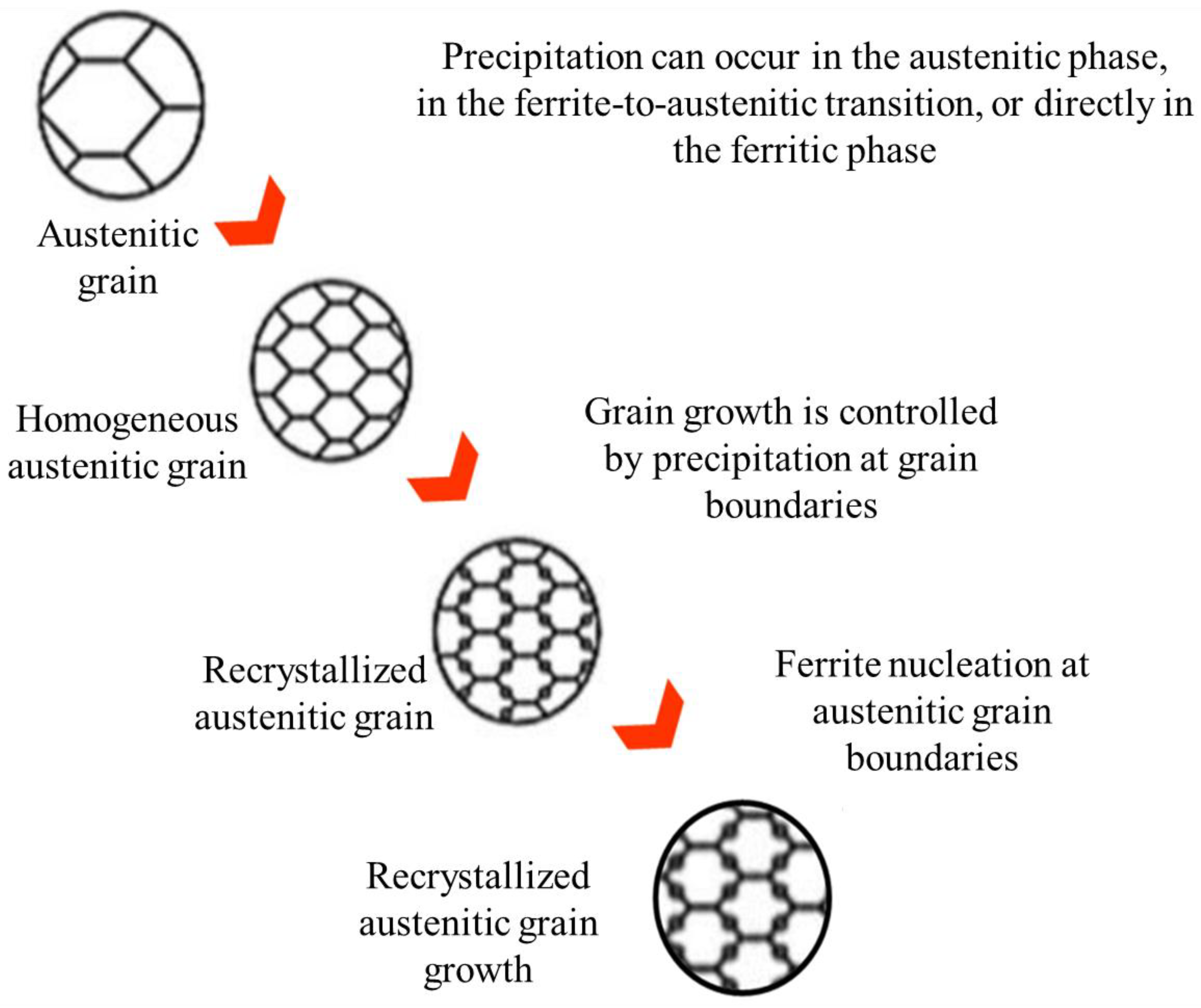
Figure 2.
a) Experimental specimen for Bahr dilatometer model DIL 805 A/D. b) Cross-sectional view. c) normal view.
Figure 2.
a) Experimental specimen for Bahr dilatometer model DIL 805 A/D. b) Cross-sectional view. c) normal view.
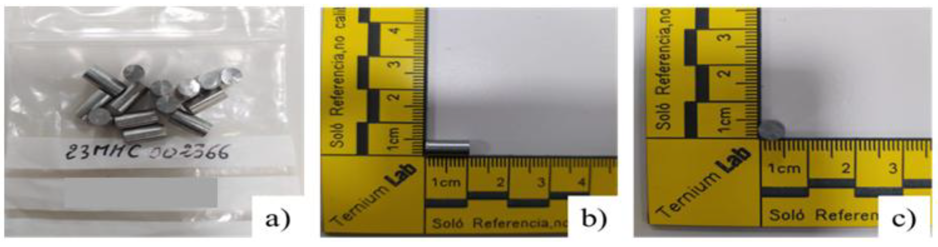
Figure 3.
Heat cycle applied to hot compression specimens for the study of precipitation.
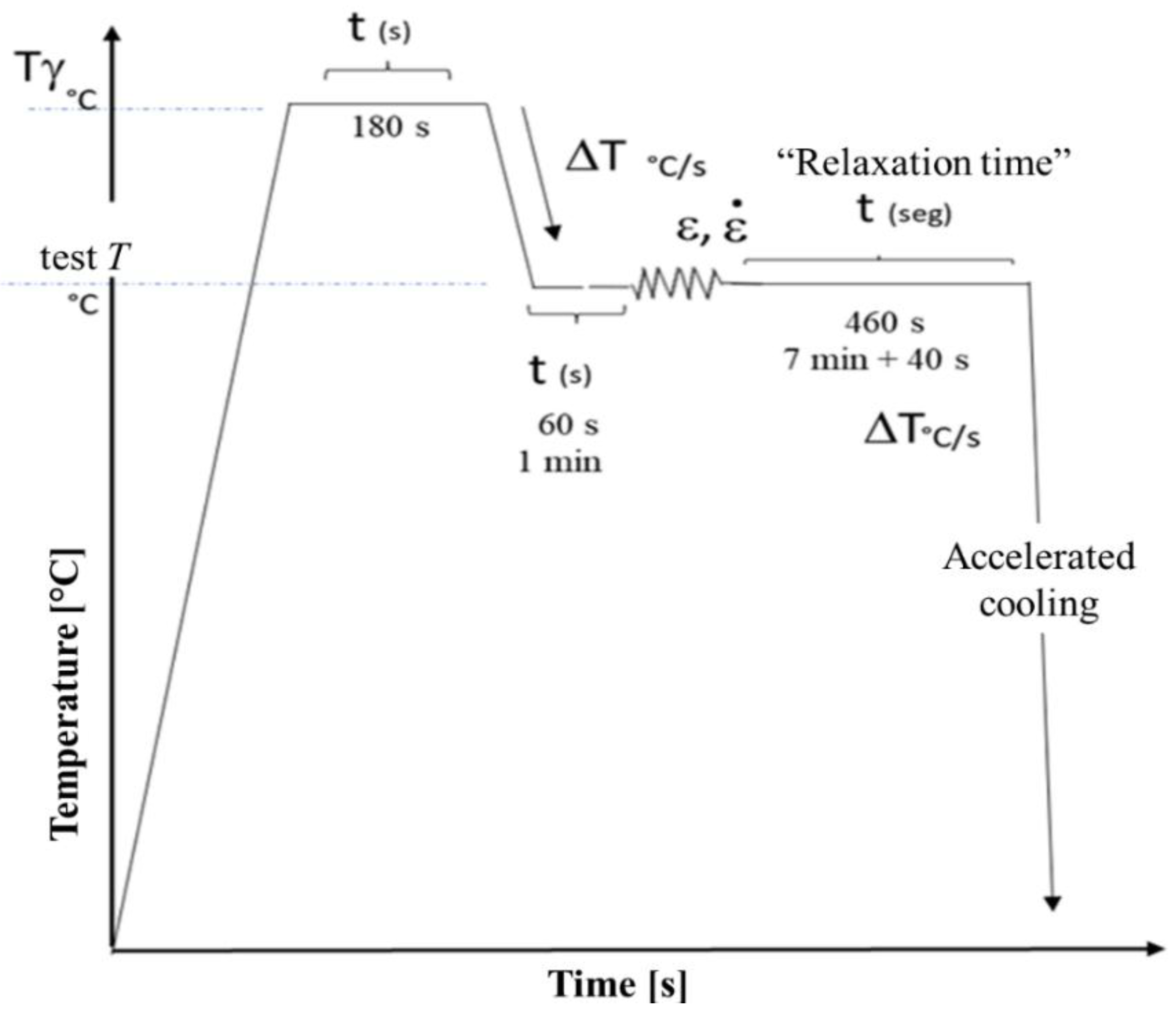
Figure 4.
Stress relaxation curve to identify the start and finish of precipitation.
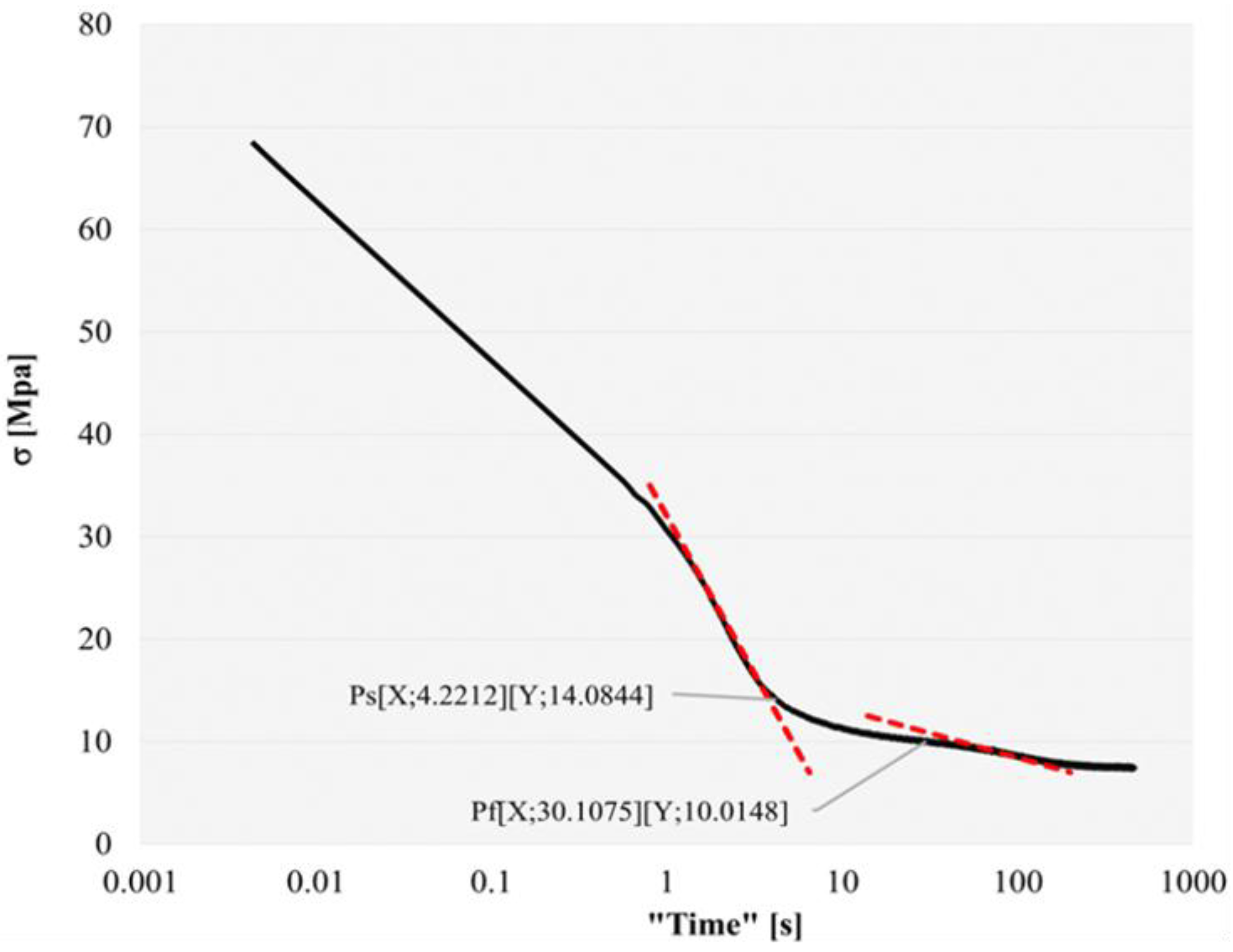
Figure 5.
Analysis area for the traceability of the characterization of the deformed microstructure of hot compression samples.
Figure 5.
Analysis area for the traceability of the characterization of the deformed microstructure of hot compression samples.
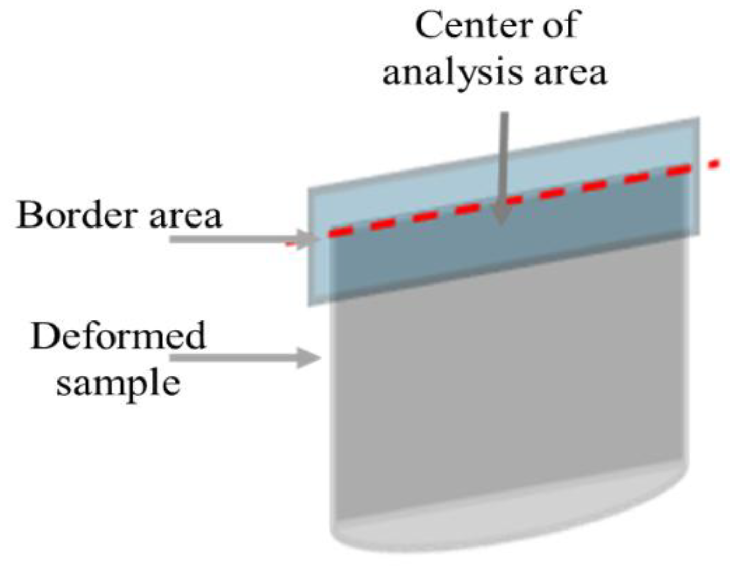
Figure 6.
Softening curves. A) 0.1Def_0.5s-1. B) 0.1Def_1s-1. C) 0.2Def_0.5s-1. D) 0.2Def_1s-1. At temperatures between 1150°C y 850°C.
Figure 6.
Softening curves. A) 0.1Def_0.5s-1. B) 0.1Def_1s-1. C) 0.2Def_0.5s-1. D) 0.2Def_1s-1. At temperatures between 1150°C y 850°C.
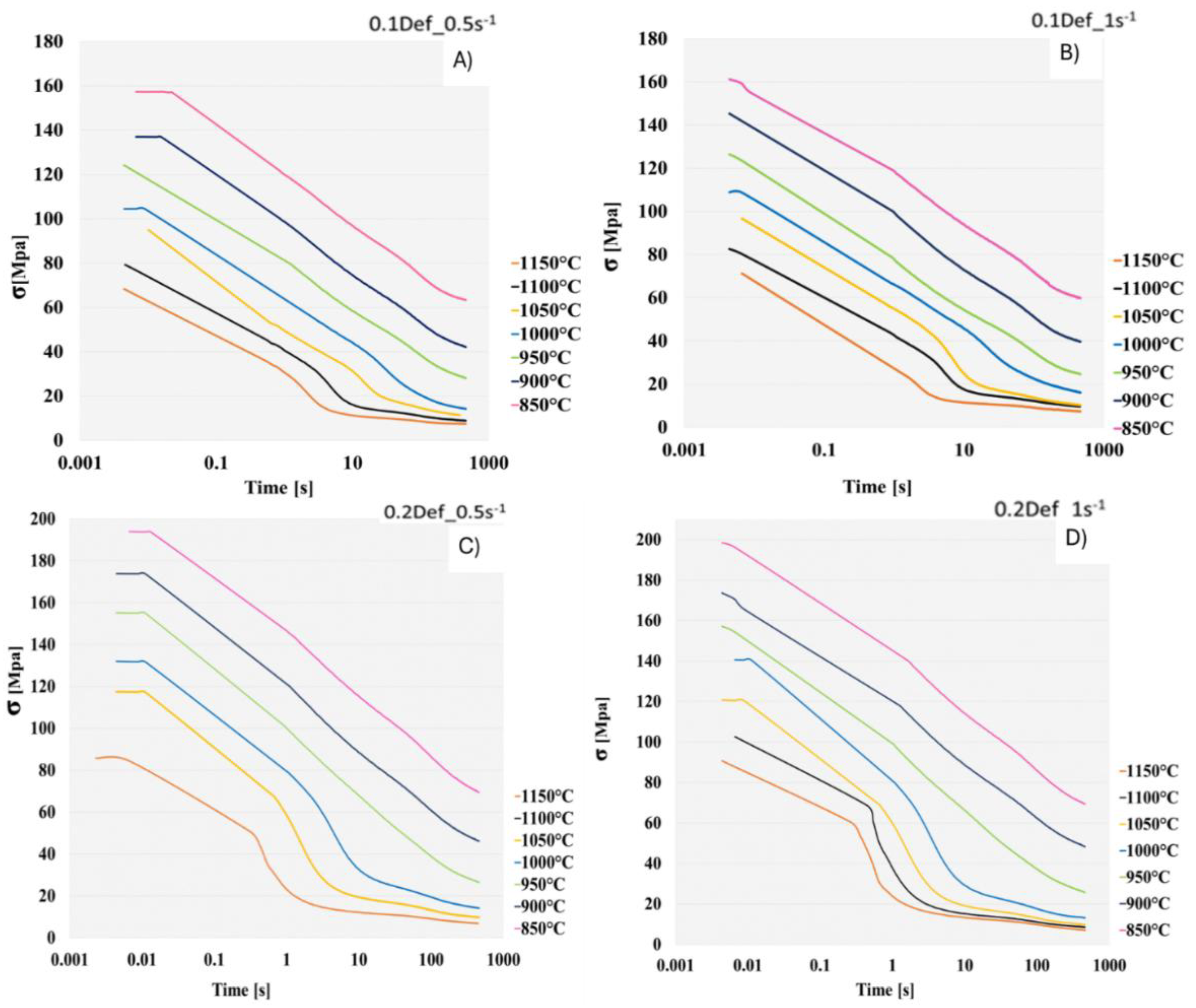
Figure 7.
Construction of experimental precipitation kinetic curves (PTT) of API steel.
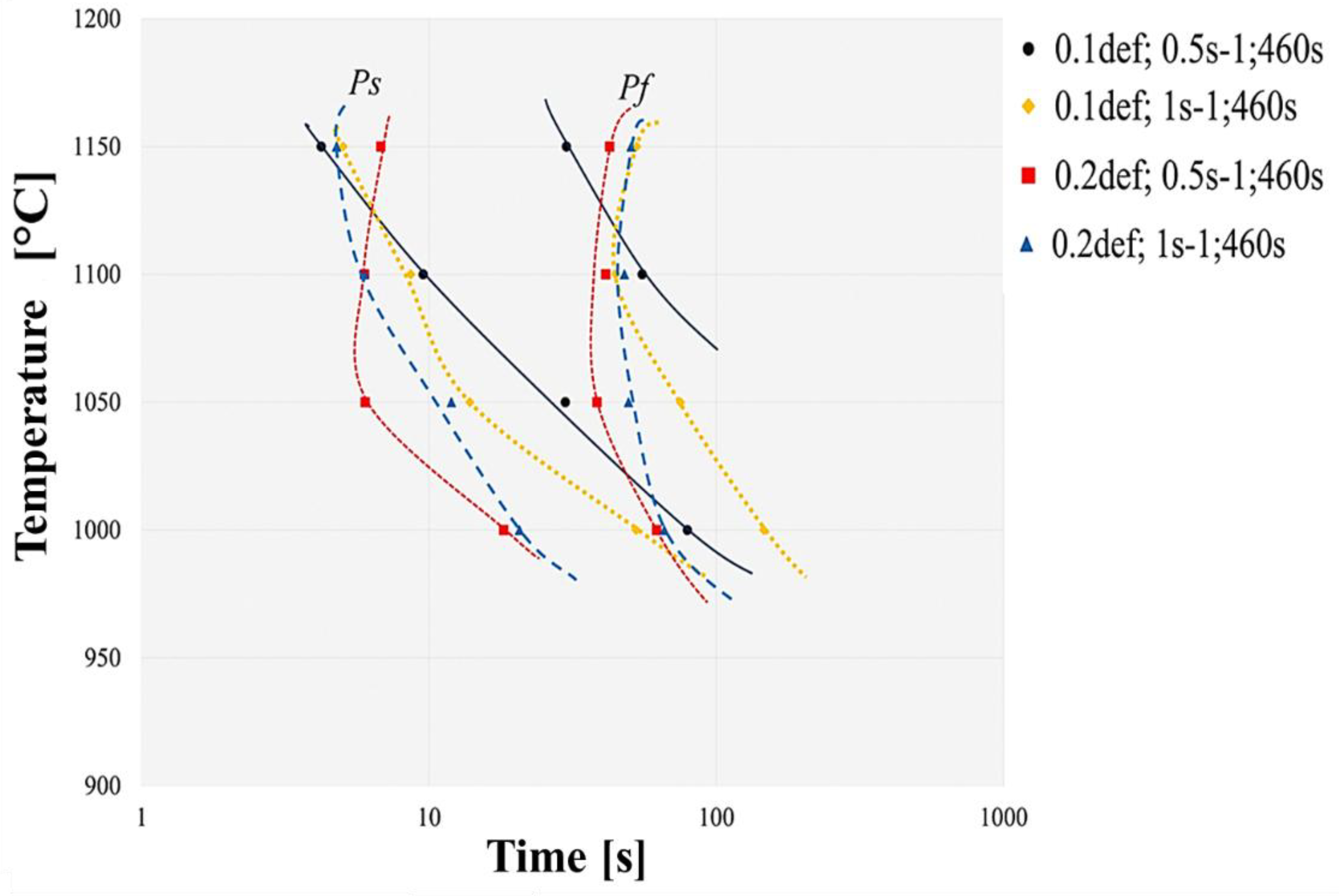
Figure 8.
Images of deformed austenitic grain boundaries developed with picric acid and hydrochloric acid solution. A) SED, B) BEDS a 2000X, 0.1 Def_0.5s-1.
Figure 8.
Images of deformed austenitic grain boundaries developed with picric acid and hydrochloric acid solution. A) SED, B) BEDS a 2000X, 0.1 Def_0.5s-1.
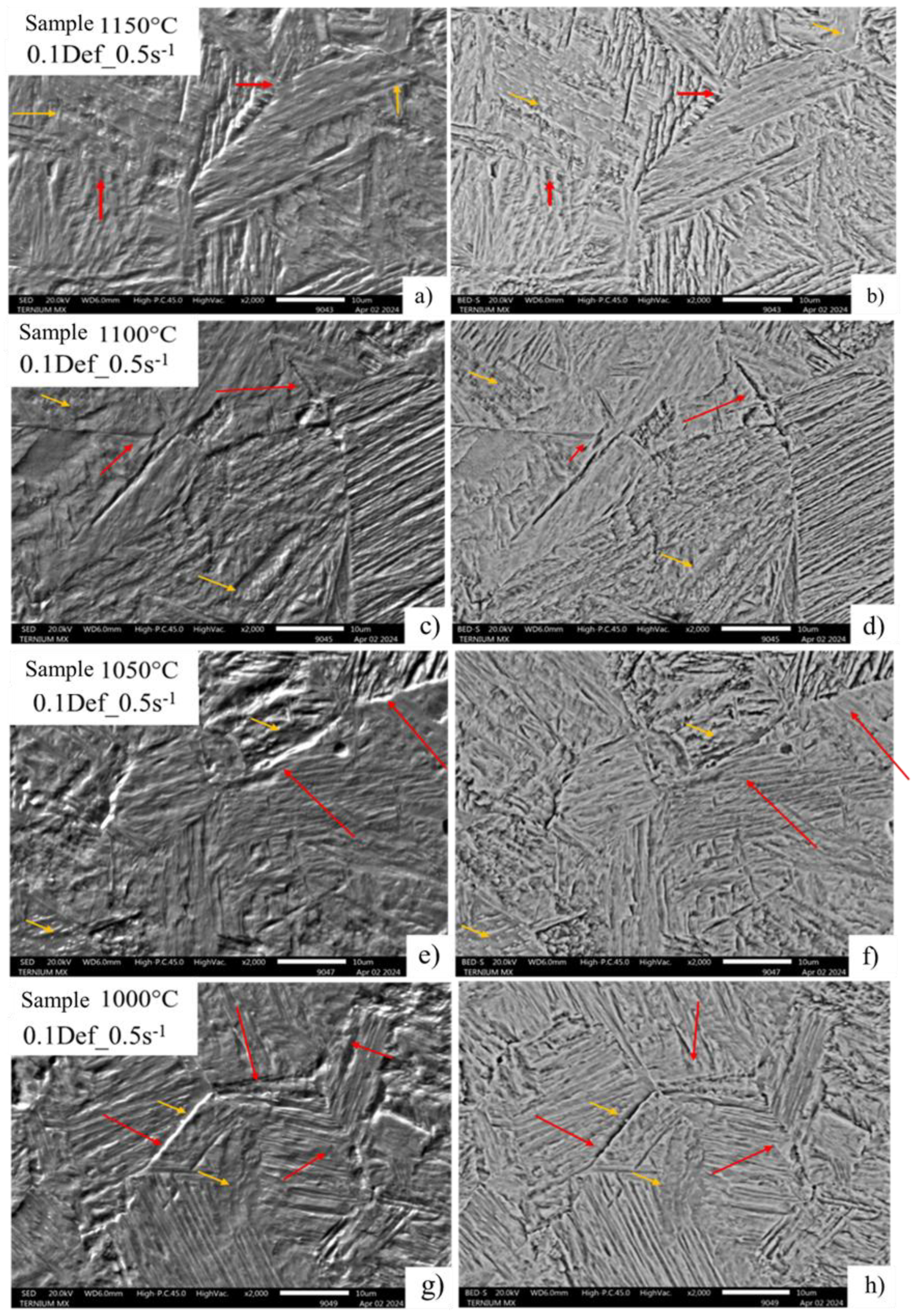
Figure 9.
Images of deformed austenitic grain boundaries developed with picric acid and hydrochloric acid solution. A) SED, B) BEDS a 2000x, 0.1 Def_1s-1.
Figure 9.
Images of deformed austenitic grain boundaries developed with picric acid and hydrochloric acid solution. A) SED, B) BEDS a 2000x, 0.1 Def_1s-1.
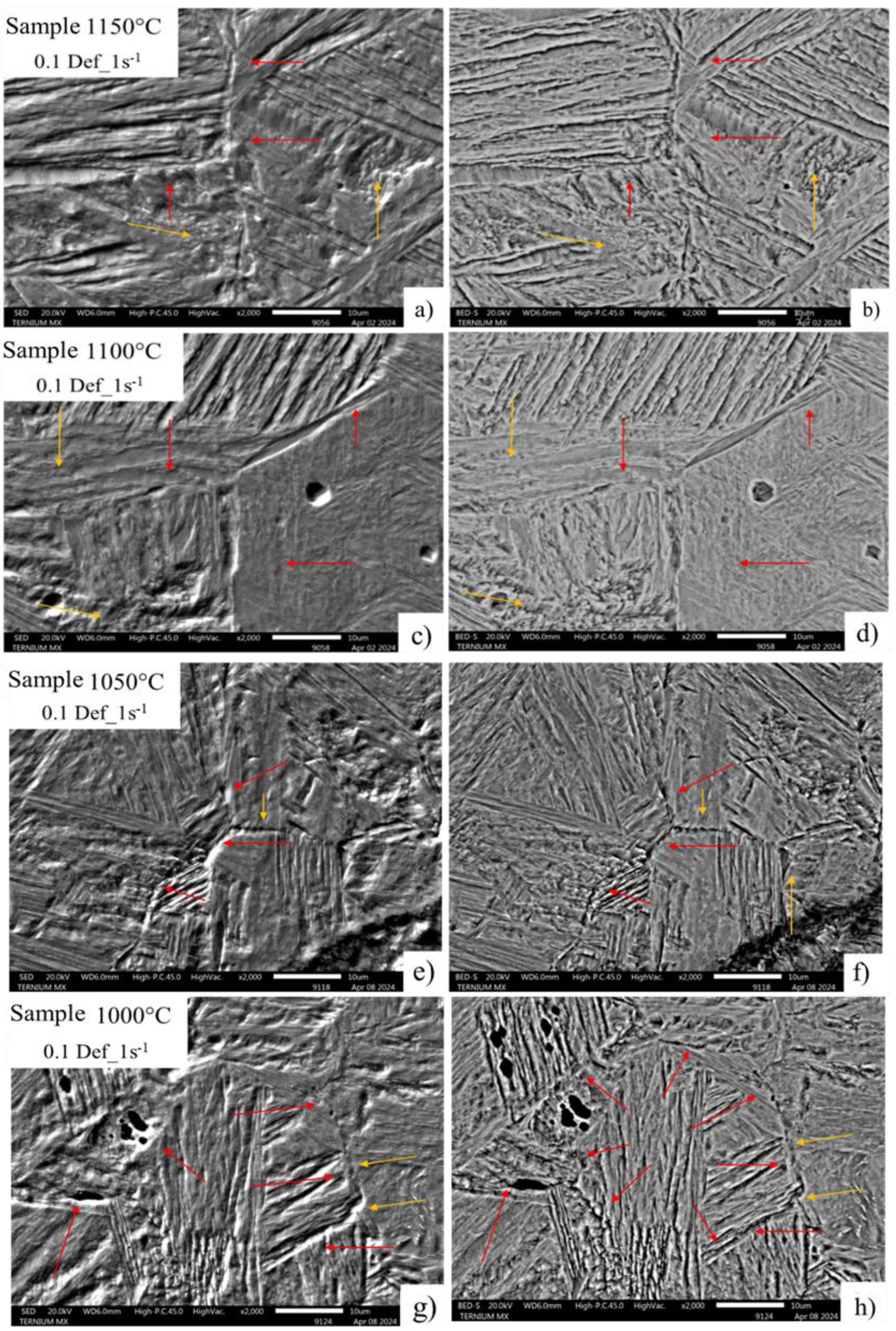
Figure 10.
Representative diagram of the behavior of the microstructure under a deformation condition of 0.1 and 1 strain rate during experimental tests.
Figure 10.
Representative diagram of the behavior of the microstructure under a deformation condition of 0.1 and 1 strain rate during experimental tests.
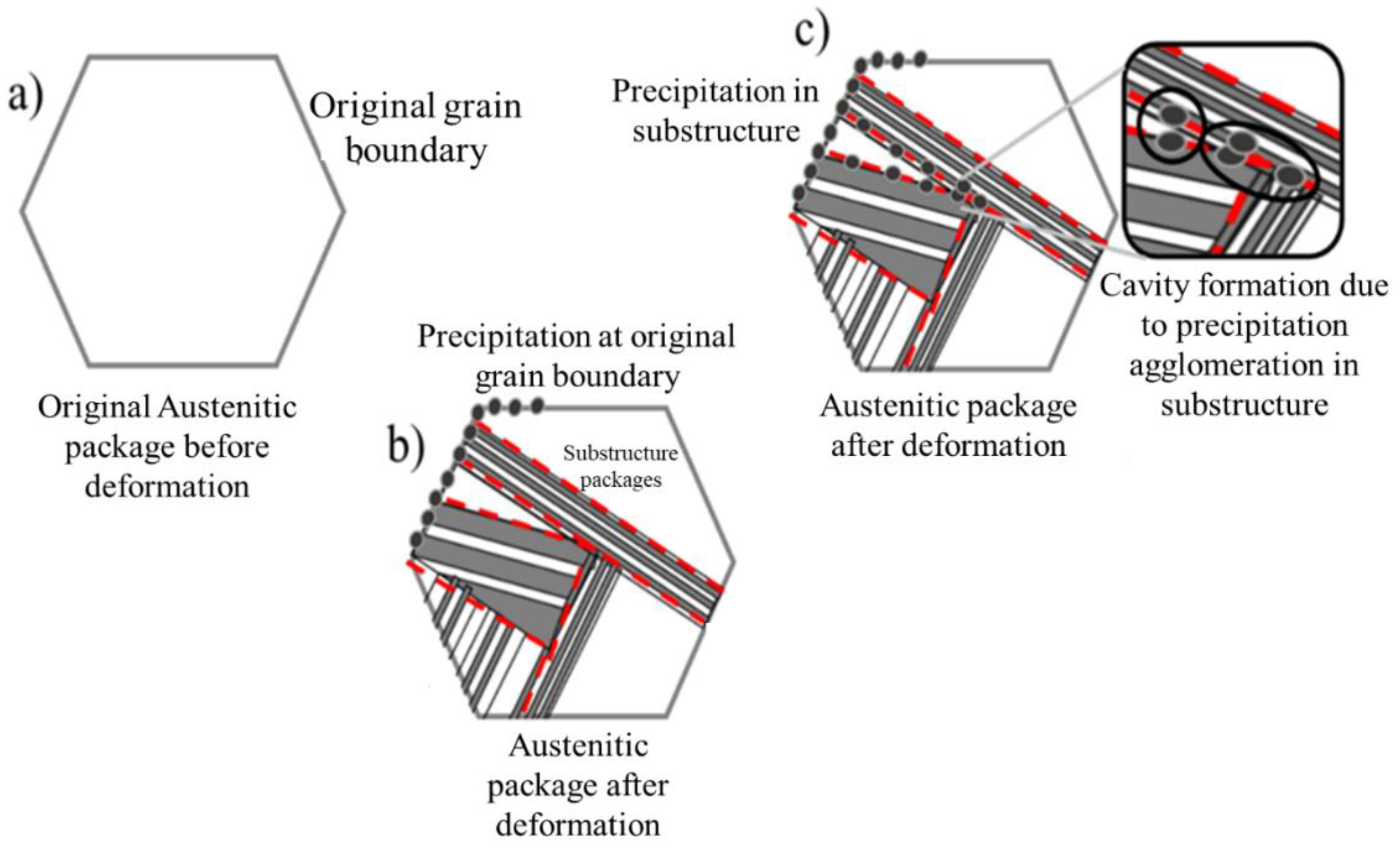
Figure 11.
Images of deformed austenitic grain boundaries developed with picric acid and hydrochloric acid solution. A) SED, B) BEDS a 2000x, 0.2 Def_0.5s-1.
Figure 11.
Images of deformed austenitic grain boundaries developed with picric acid and hydrochloric acid solution. A) SED, B) BEDS a 2000x, 0.2 Def_0.5s-1.
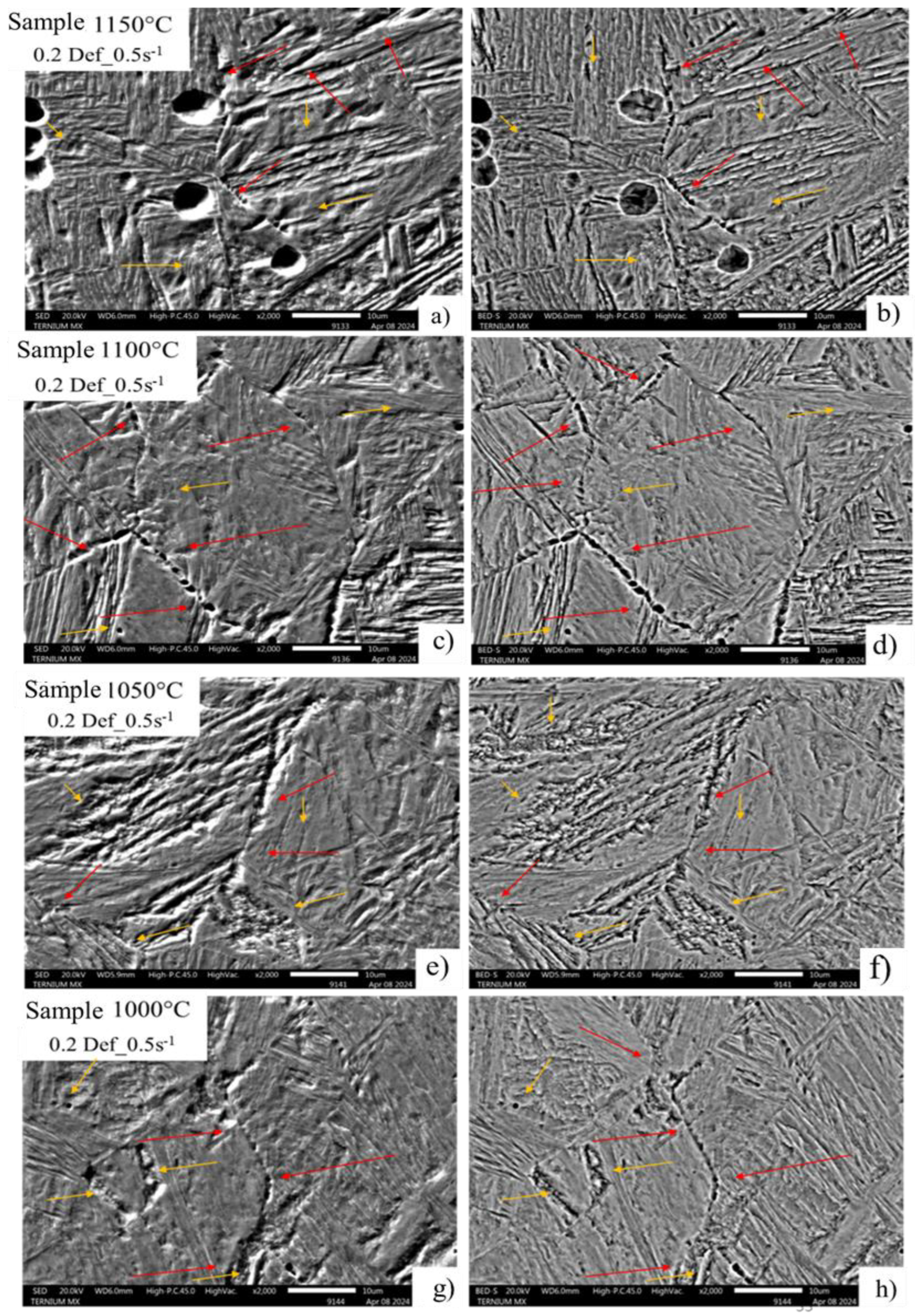
Figure 12.
Images of deformed austenitic grain boundaries developed with picric acid and hydrochloric acid solution. A) SED, B) BEDS a 2000x, 0.2 Def_1s-1.
Figure 12.
Images of deformed austenitic grain boundaries developed with picric acid and hydrochloric acid solution. A) SED, B) BEDS a 2000x, 0.2 Def_1s-1.
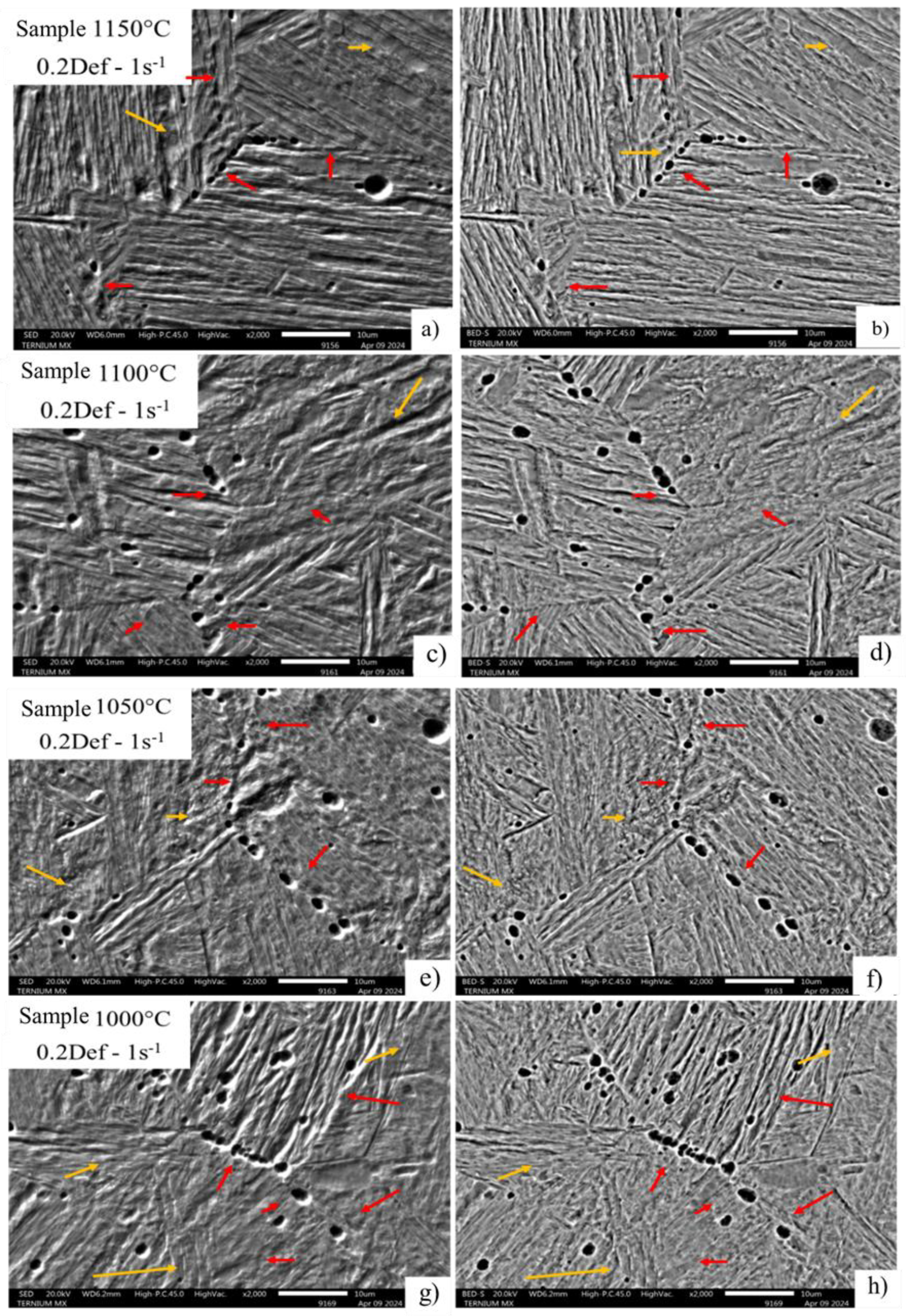
Figure 13.
MO image of thickening of deformed austenitic grain boundaries revealed with chemical attack of picric acid and hydrochloric acid of the condition 0.1def 0.5s-1.
Figure 13.
MO image of thickening of deformed austenitic grain boundaries revealed with chemical attack of picric acid and hydrochloric acid of the condition 0.1def 0.5s-1.
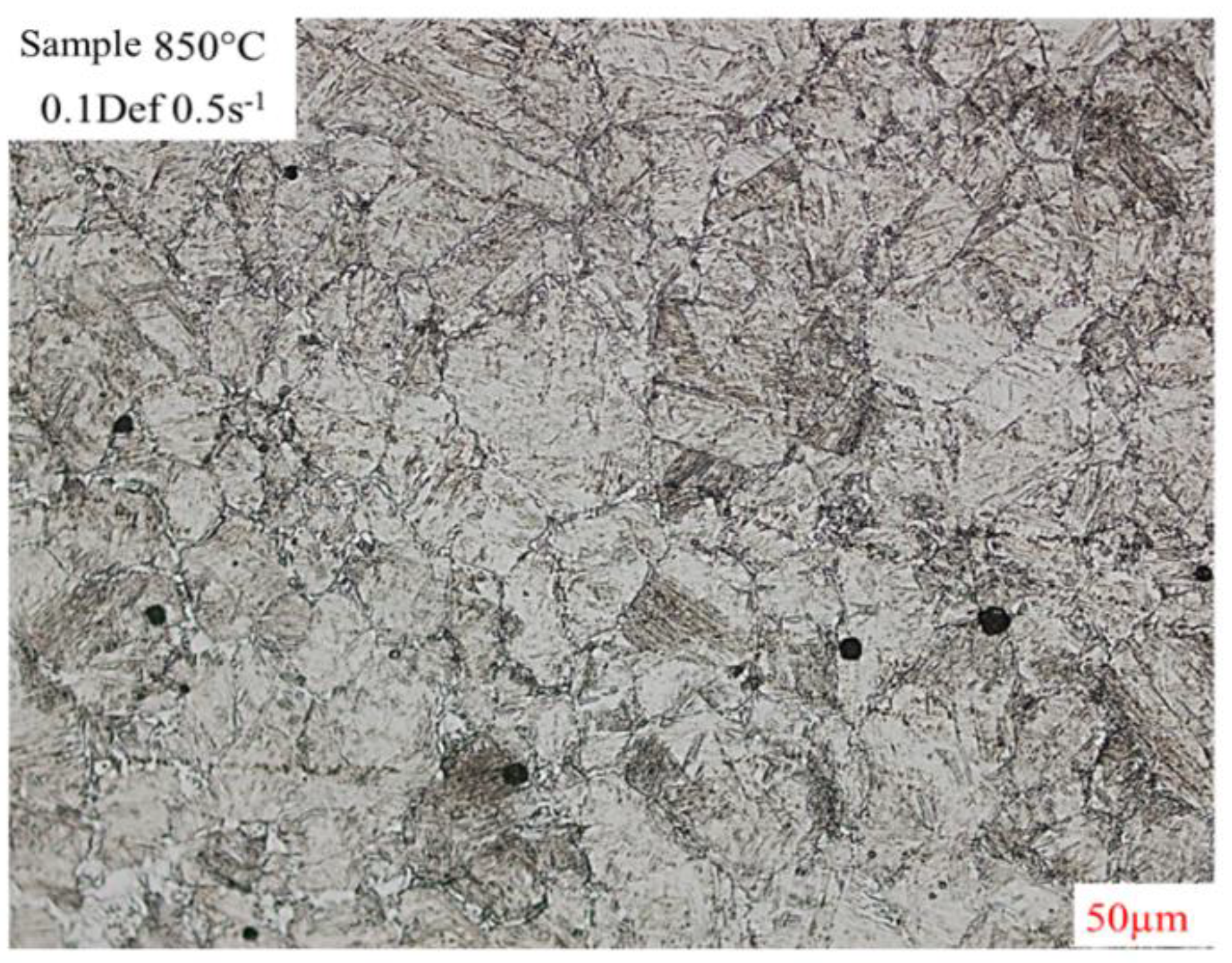
Figure 14.
Thickening of deformed austenitic grain boundaries at 850°C, developed with picric and hydrochloric acid solution. A) SED, B) BEDS, 0.1 Def_0.5s-1.
Figure 14.
Thickening of deformed austenitic grain boundaries at 850°C, developed with picric and hydrochloric acid solution. A) SED, B) BEDS, 0.1 Def_0.5s-1.
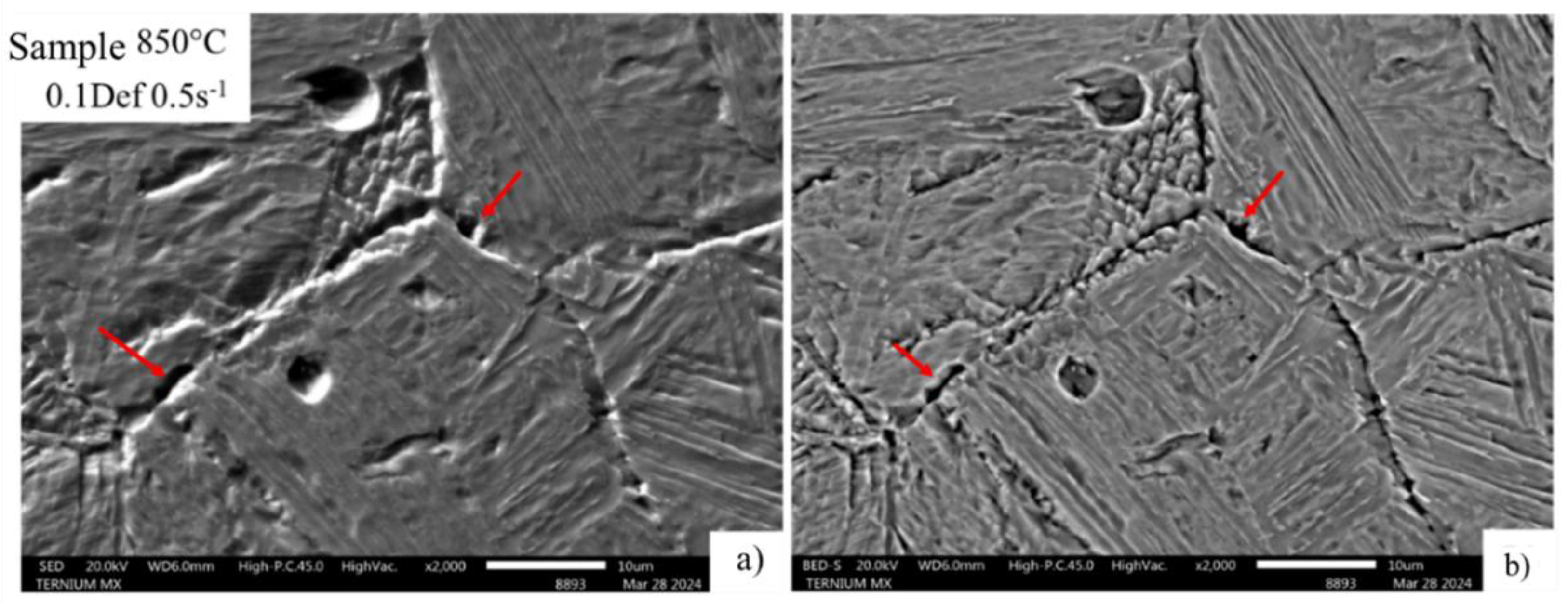
Figure 15.
Thickening of deformed austenitic grain boundaries at 850°C, developed with picric and hydrochloric acid solution. A) SED, B) BEDS, 0.2 Def_1s-1.
Figure 15.
Thickening of deformed austenitic grain boundaries at 850°C, developed with picric and hydrochloric acid solution. A) SED, B) BEDS, 0.2 Def_1s-1.
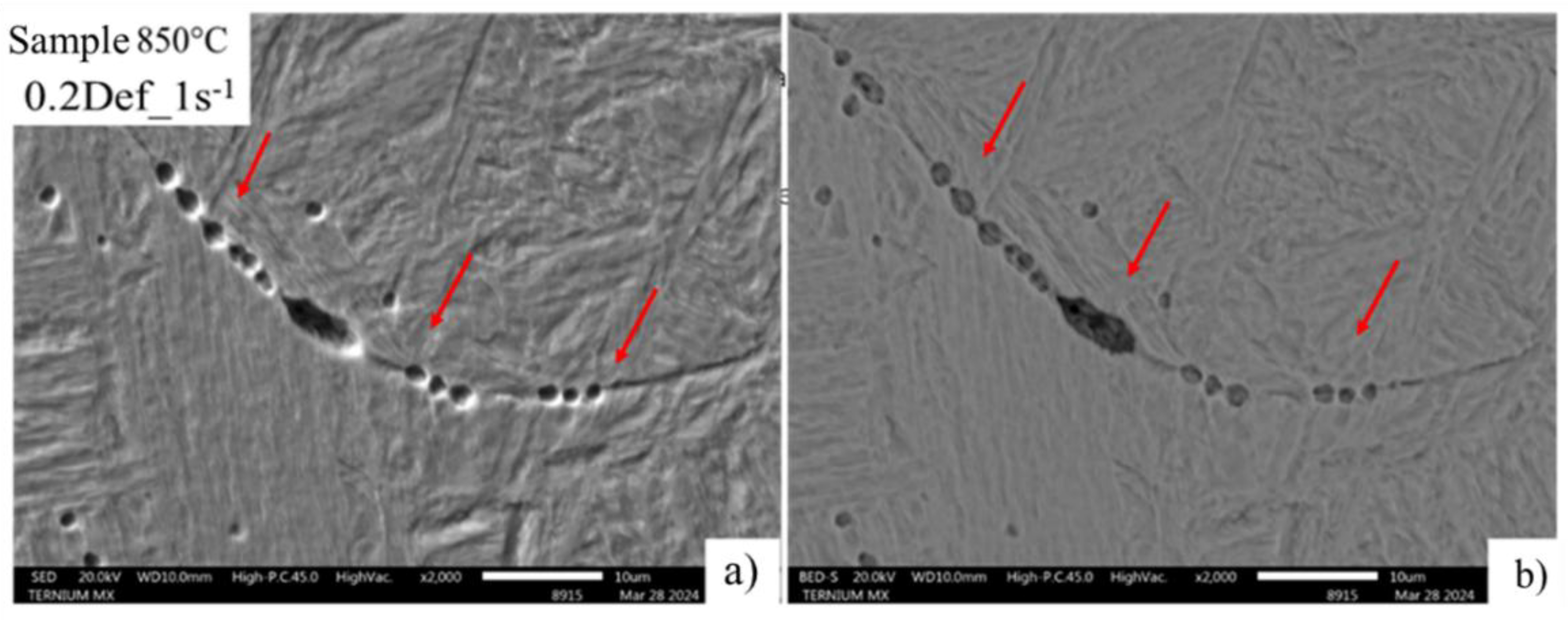
Figure 16.
Ferrite formation in deformation-induced precipitation zone with form decreases temperature.
Figure 16.
Ferrite formation in deformation-induced precipitation zone with form decreases temperature.
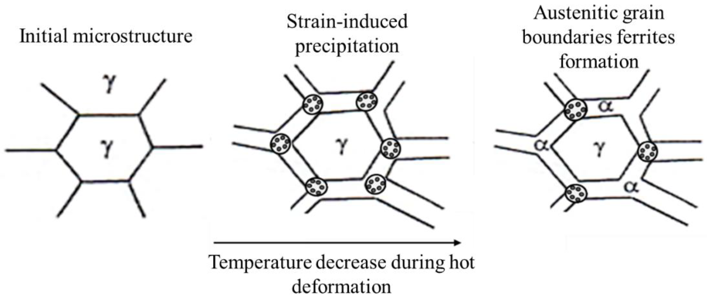
Figure 17.
Brightfield (BF) image of precipitation in the microstructure of condition 2. a) Substructure with localized precipitation. b) Colony of nano precipitates. c) Precipitation interface at substructure and matrix boundary.
Figure 17.
Brightfield (BF) image of precipitation in the microstructure of condition 2. a) Substructure with localized precipitation. b) Colony of nano precipitates. c) Precipitation interface at substructure and matrix boundary.
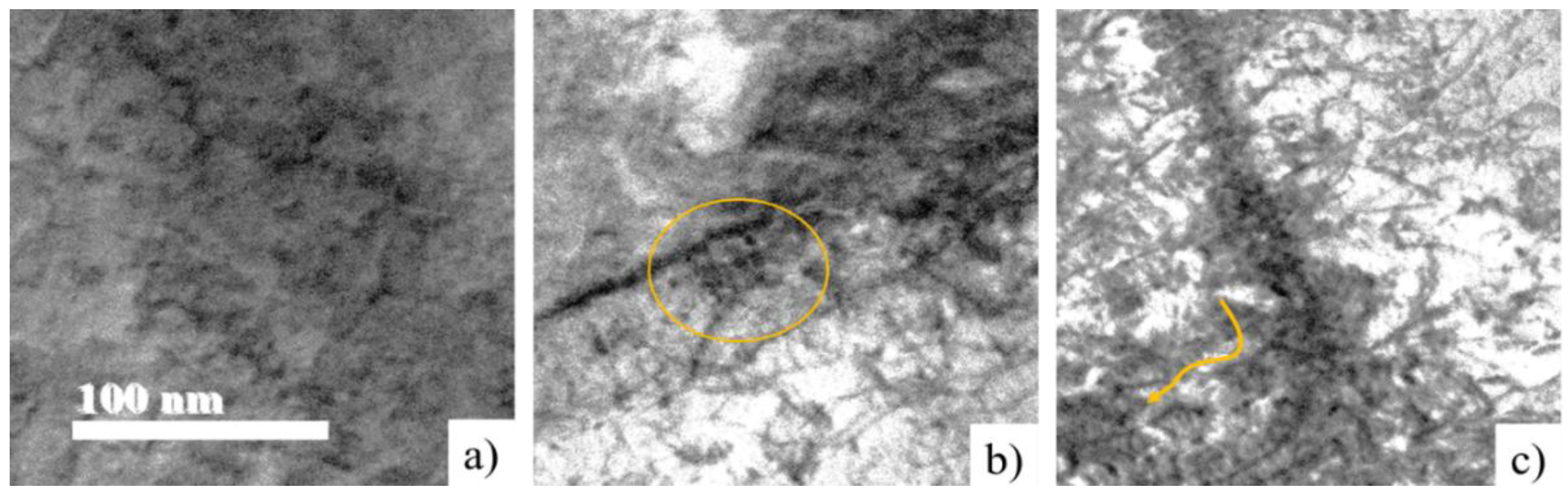
Figure 18.
Brightfield (BF) image of condition 3. c) Distribution of nanoprecipitation in the substructure. b) Coherent interface with brindle accommodation. c) Linear arrangement of precipitation in the steel matrix.
Figure 18.
Brightfield (BF) image of condition 3. c) Distribution of nanoprecipitation in the substructure. b) Coherent interface with brindle accommodation. c) Linear arrangement of precipitation in the steel matrix.
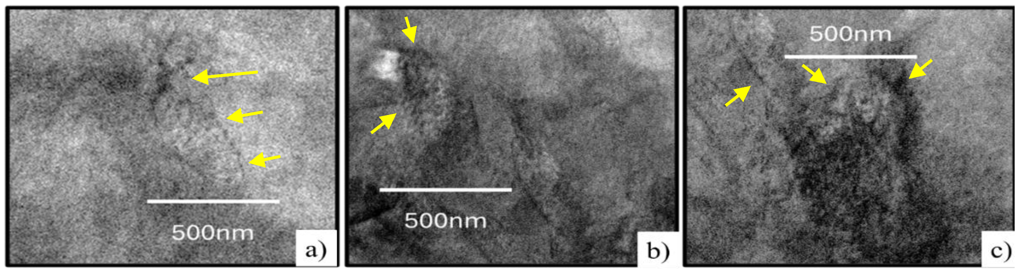
Figure 19.
Darkfield (DF) image of condition 3 at 5 nm magnification. a) Measurement of the atomic covalent radius that distinguishes the nanoprecipitate.
Figure 19.
Darkfield (DF) image of condition 3 at 5 nm magnification. a) Measurement of the atomic covalent radius that distinguishes the nanoprecipitate.
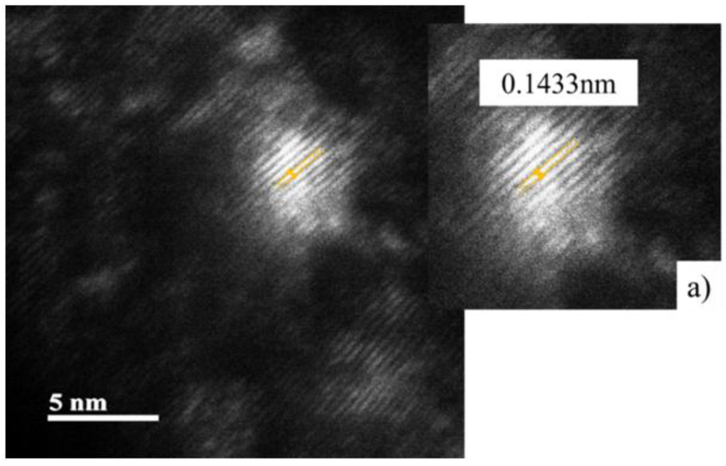
Figure 20.
Brightfield image of condition 4 to 1μm representing the extended planar type interface in the steel matrix.
Figure 20.
Brightfield image of condition 4 to 1μm representing the extended planar type interface in the steel matrix.
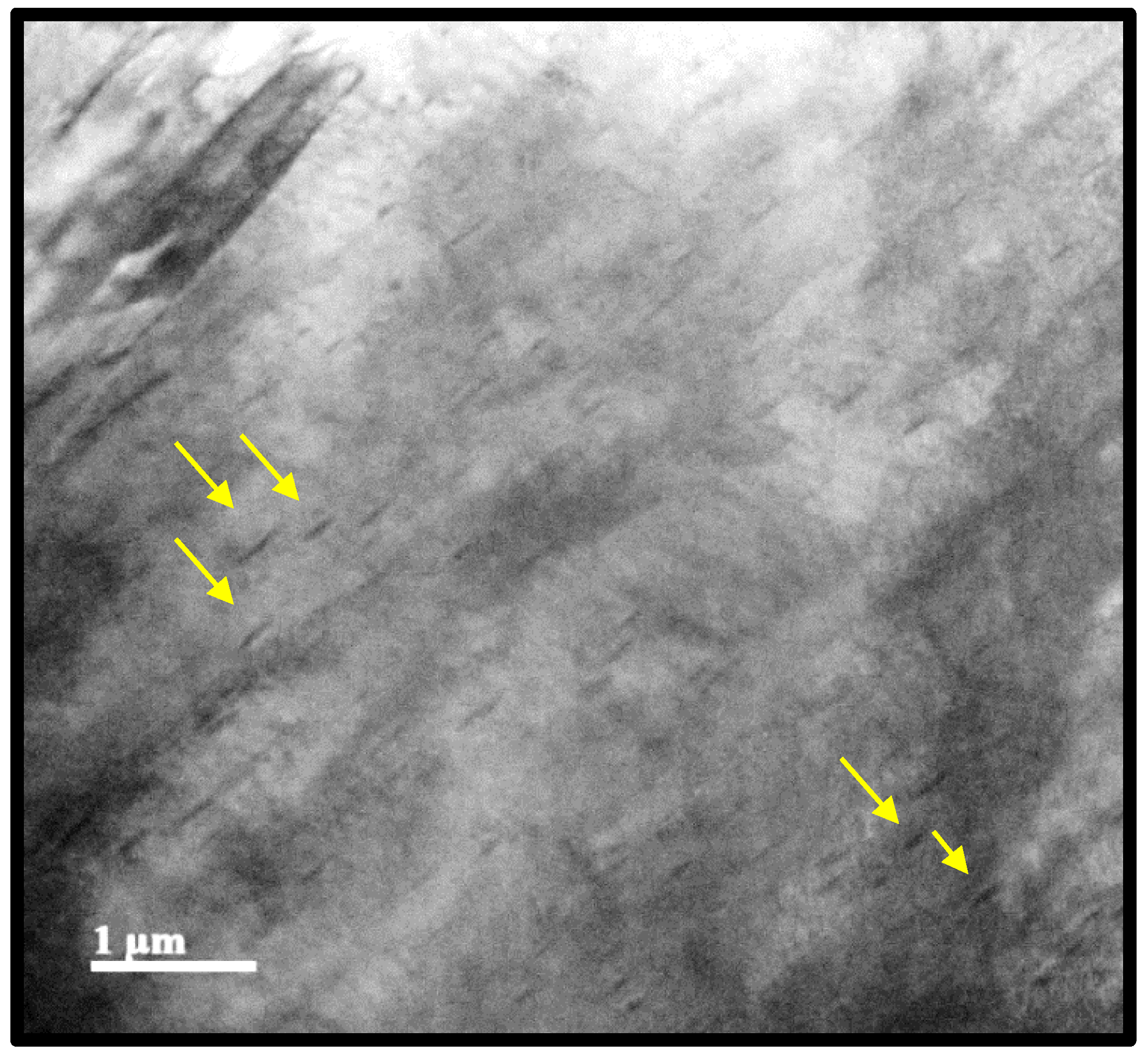
Figure 21.
Dark Field (DF) Images of Condition 4. a) Nano precipitates of 3 to 5 nm at the substructure limit. (b) and (c) Measurement of atomic radius in high-resolution precipitate.
Figure 21.
Dark Field (DF) Images of Condition 4. a) Nano precipitates of 3 to 5 nm at the substructure limit. (b) and (c) Measurement of atomic radius in high-resolution precipitate.
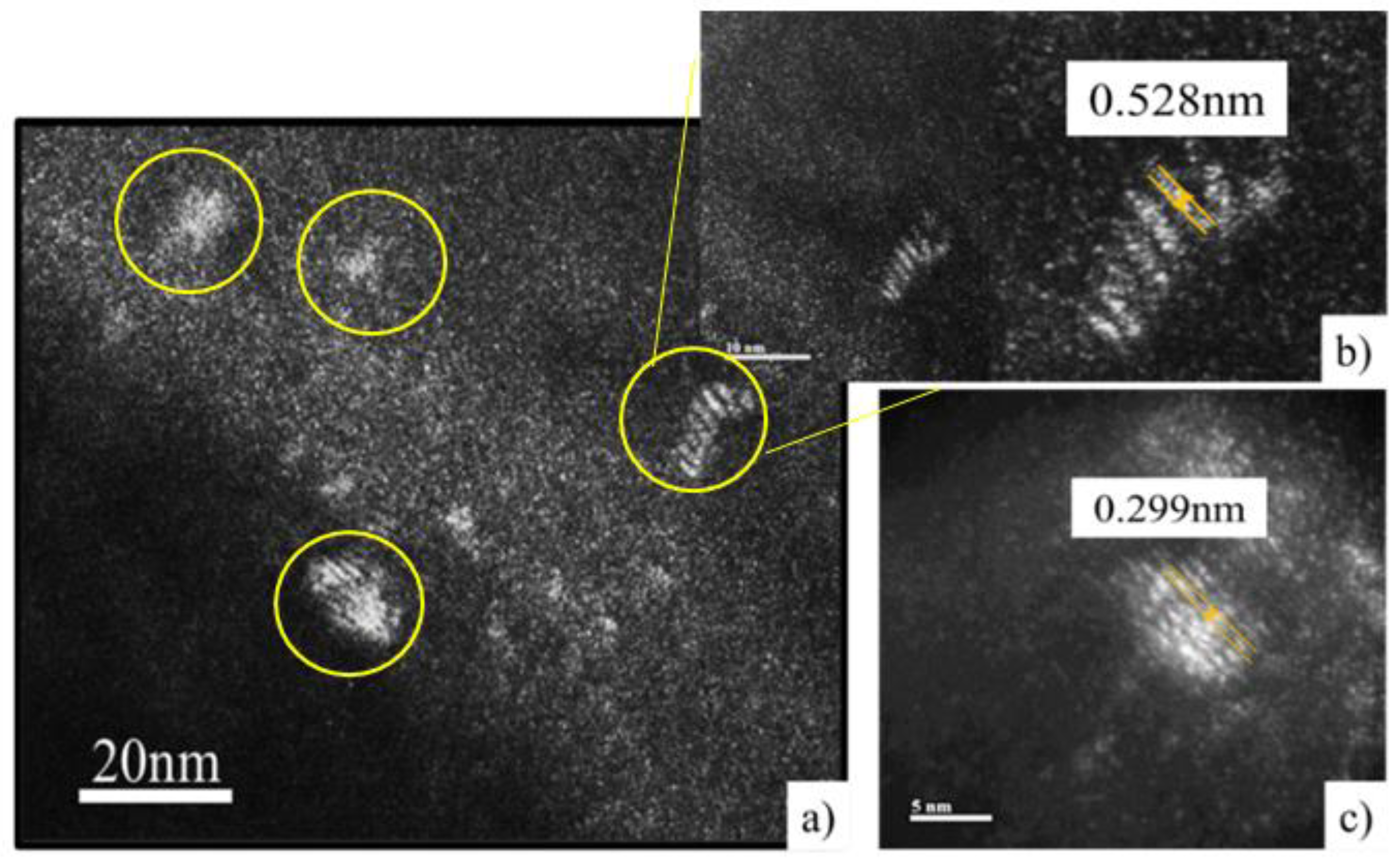
Figure 22.
Dark field image of analyzed areas by electron diffraction to determine the constitution of precipitation in condition 2.
Figure 22.
Dark field image of analyzed areas by electron diffraction to determine the constitution of precipitation in condition 2.
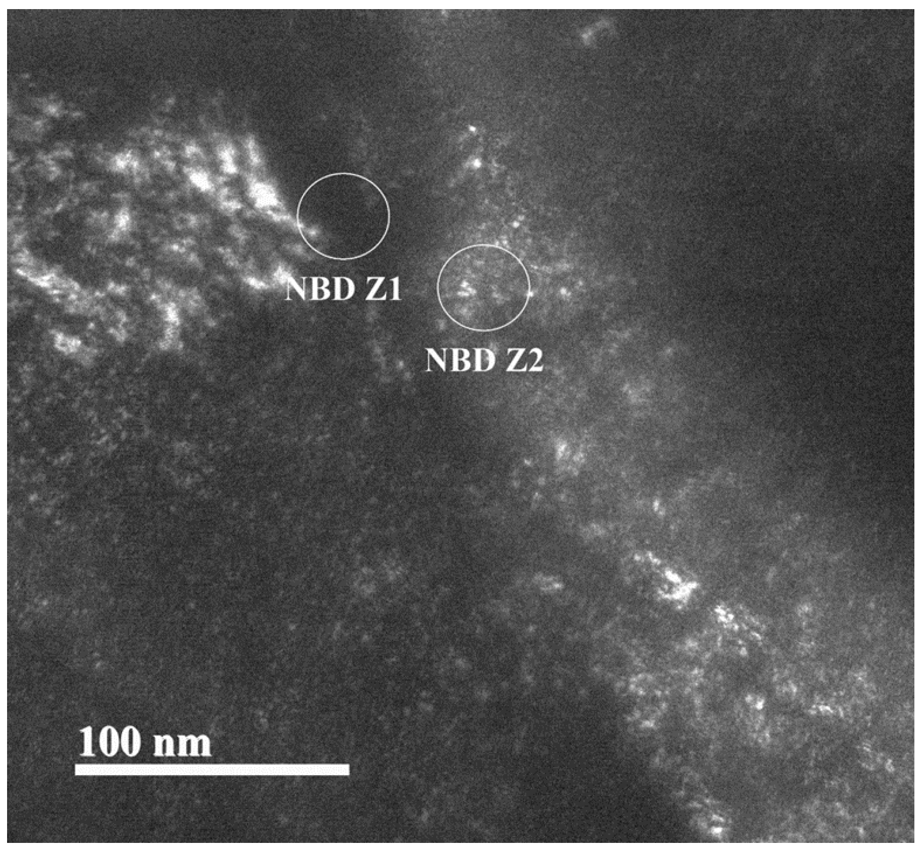
Figure 23.
Analysis of the diffraction pattern of Z1 for matrix identification.
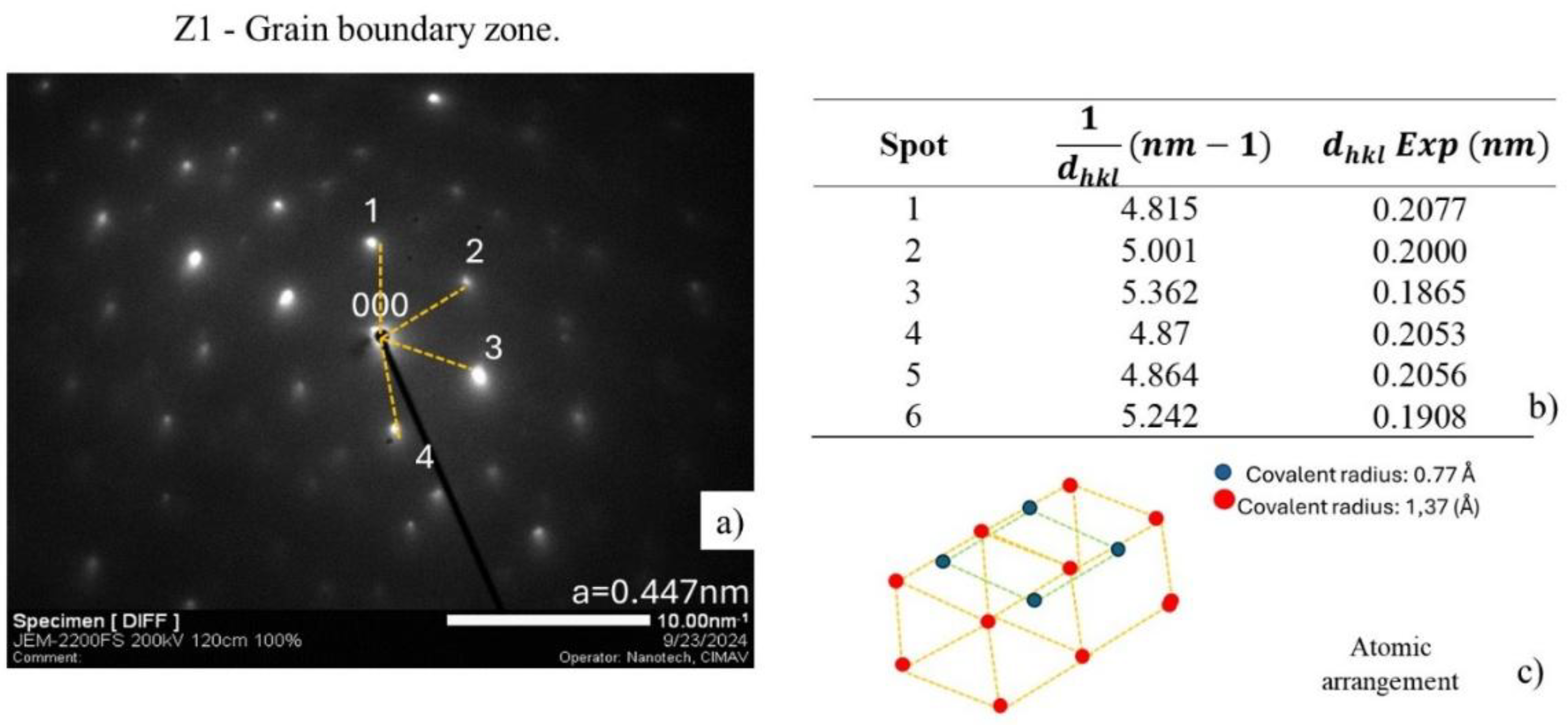
Figure 24.
Identification of the constitution of the deformation-induced precipitate with coherent interface with the matrix.
Figure 24.
Identification of the constitution of the deformation-induced precipitate with coherent interface with the matrix.
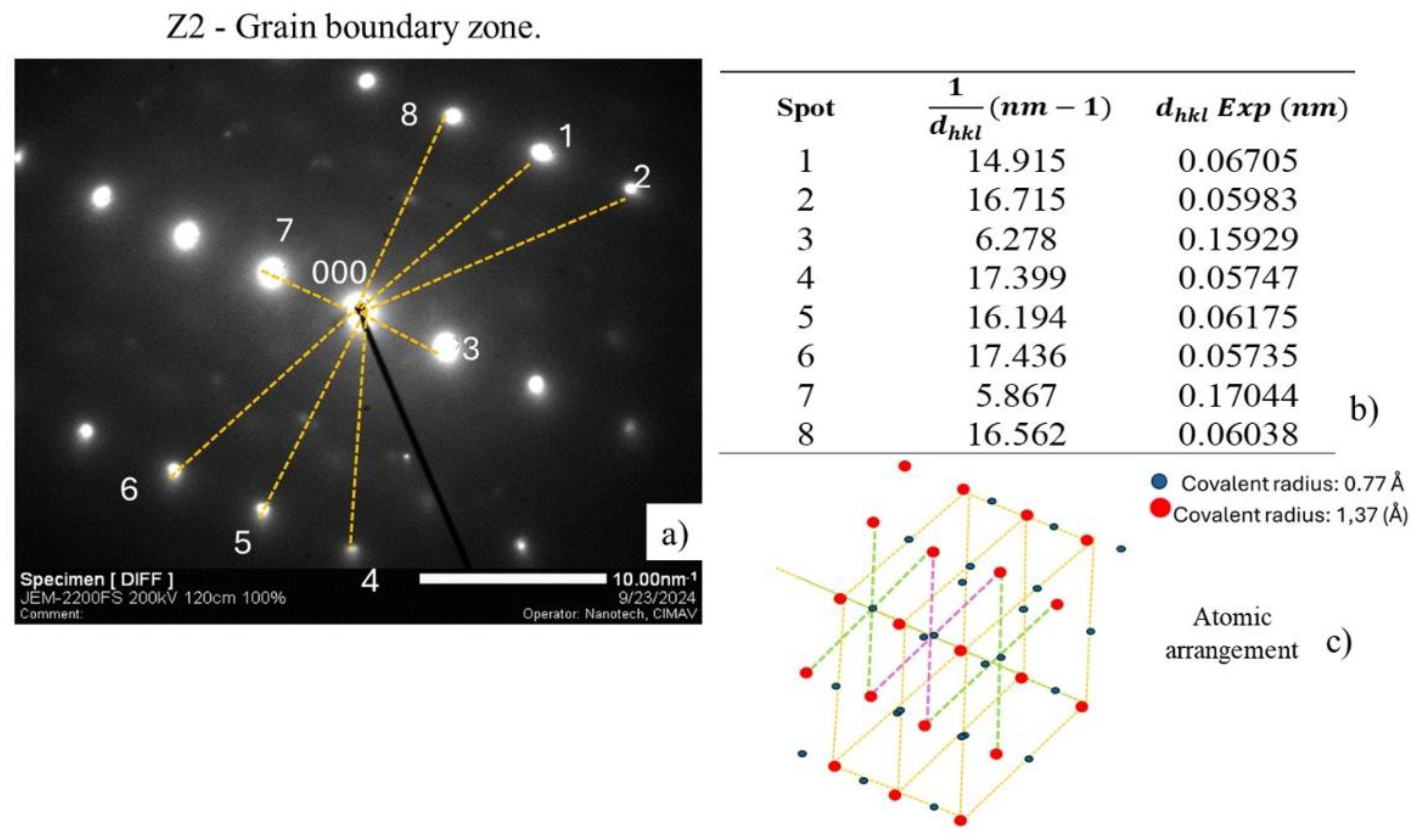
Figure 25.
Determination of the precipitation mechanism for the steel from experimental testing and microstructural characterization (MEB, EBSD, TEM).
Figure 25.
Determination of the precipitation mechanism for the steel from experimental testing and microstructural characterization (MEB, EBSD, TEM).
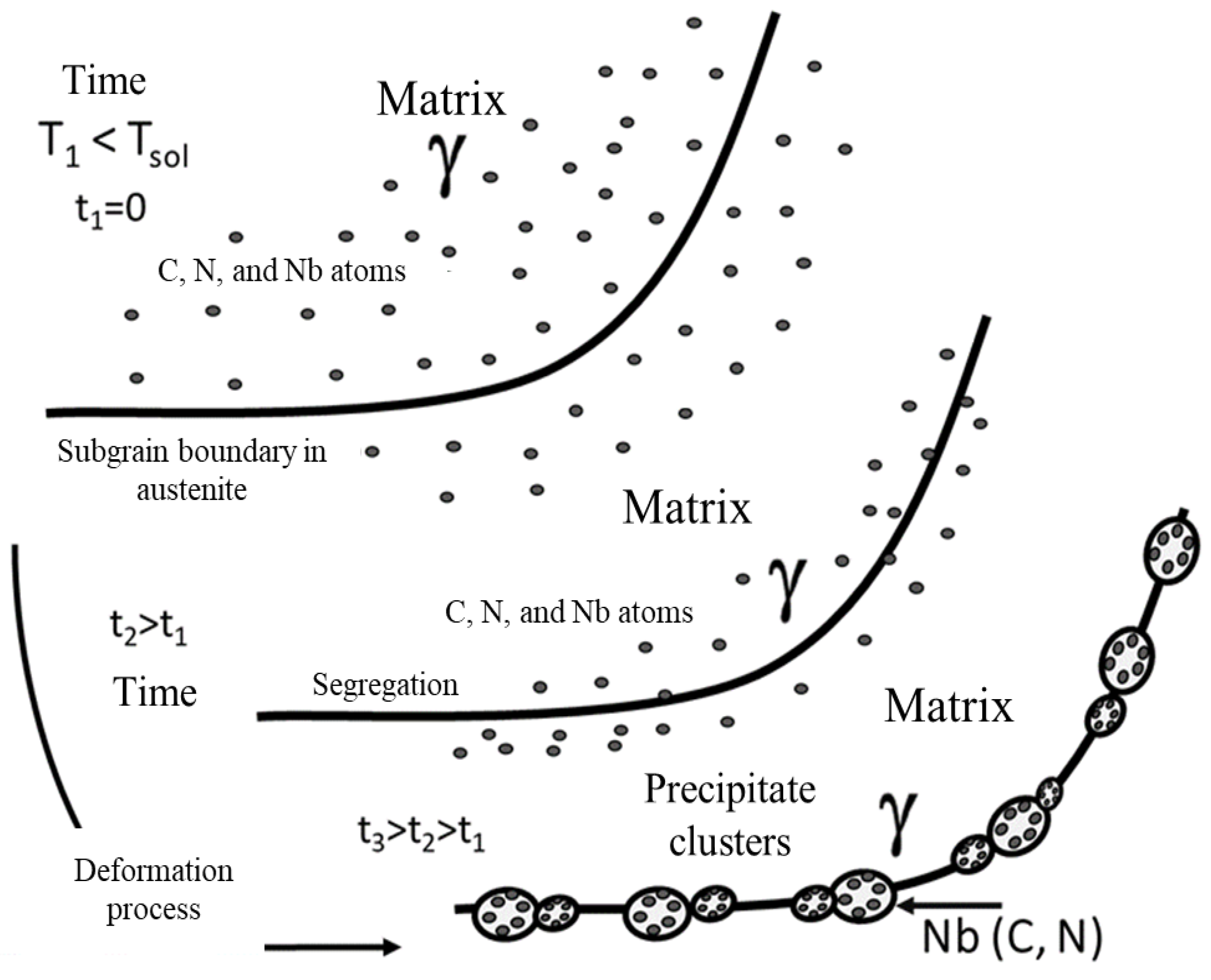

Table 1.
Chemical composition of API steel.
| C | Nb | Cr | P | Mn | Mo | Si | Ti | V | |
| Wt% | < 0.09 | < 0.050 | < 0.3 | 0.016 | 1.67 | < 0.006 | 0.25 | < 0.015 | <0.005 |
Table 2.
Compilation of the start (Ps) and finish (Pf) points of precipitation of the curves obtained from the hot compression tests with stress relaxation.
Table 2.
Compilation of the start (Ps) and finish (Pf) points of precipitation of the curves obtained from the hot compression tests with stress relaxation.
| Temperature | Start (Ps) | Finish (Pf) | |
| 0.1 strain; 0.5s-1;460s | 1150 1100 1050 1000 950 900 850 |
4.2 9.5 29.8 79.3 - - - |
30.1 55.2 - - - - - |
| 0.1 strain; 1s-1;460s | 1150 1100 1050 1000 950 900 850 |
5.0 8.6 13.8 52.5 - - - |
52.8 44.7 75.0 146.2 - - - |
| 0.2 strain; 0.5s-1;460s | 1150 1100 1050 1000 950 900 850 |
6.8 5.9 5.9 18.2 - - - |
42.5 41.2 38.4 61.9 - - - |
| 0.2 strain; 1s-1;460s | 1150 1100 1050 1000 950 900 850 |
4.7 5.9 11.9 20.6 - - - |
50.6 47.9 49.5 65.9 - - - |
Table 3.
Experimental vs. theoretical comparison for plane identification for each spot in Z1.
| Puntos | Plano Candidato | |||
|---|---|---|---|---|
| 1 | 4.815 | 0.2077 | 0.2235 | (200) |
| 2 | 5.001 | 0.2000 | 0.2000 | (210) |
| 3 | 5.362 | 0.1865 | 0.1865 | (211) |
| 4 | 4.87 | 0.2053 | 0.2235 | (200) |
| 5 | 4.864 | 0.2056 | 0.2235 | (200) |
| 6 | 5.242 | 0.1908 | 0.1908 | (310) |
Table 4.
Experimental vs. theoretical comparison for plane identification for each spot in Z2.
| Spot | Candidate Plane | Difference (%) | |||
|---|---|---|---|---|---|
| 1 | 14.915 | 0.0670 | 0.0645 | (444) | 3.88% |
| 2 | 16.715 | 0.0598 | 0.0597 | (622) | 0.17% |
| 3 | 6.278 | 0.1593 | 0.1581 | (220) | 0.76% |
| 4 | 17.399 | 0.0575 | 0.0597 | (622) | 3.68% |
| 5 | 16.194 | 0.0618 | 0.0620 | (620) | 0.32% |
| 6 | 17.436 | 0.0574 | 0.0597 | (622) | 3.85% |
| 7 | 5.867 | 0.1704 | 0.1581 | (220) | 7.78% |
| 8 | 16.562 | 0.0604 | 0.0620 | (620) | 2.58% |
Disclaimer/Publisher’s Note: The statements, opinions and data contained in all publications are solely those of the individual author(s) and contributor(s) and not of MDPI and/or the editor(s). MDPI and/or the editor(s) disclaim responsibility for any injury to people or property resulting from any ideas, methods, instructions or products referred to in the content. |
© 2025 by the authors. Licensee MDPI, Basel, Switzerland. This article is an open access article distributed under the terms and conditions of the Creative Commons Attribution (CC BY) license (http://creativecommons.org/licenses/by/4.0/).
Copyright: This open access article is published under a Creative Commons CC BY 4.0 license, which permit the free download, distribution, and reuse, provided that the author and preprint are cited in any reuse.


